
Precision and Accuracy of Pulse Propagation Velocity Measurement in Power Cables


Department of Electrical Power Engineering and Mechatronics, Tallinn University of Technology, 19086 Tallinn, Estonia
*
Authors to whom correspondence should be addressed.
Energies 2023, 16(6), 2702; https://doi.org/10.3390/en16062702
Submission received: 19 January 2023
/
Revised: 8 March 2023
/
Accepted: 10 March 2023
/
Published: 14 March 2023
(This article belongs to the Special Issue Condition Monitoring of Power System Components)
Abstract
:The partial discharge (PD) measurement is an important method used in determining the condition of medium- and high-voltage cable insulation. Considering the propagation velocity of PD signals in power cables is necessary for determining the location of PD defects. However, the determination of velocity is not straightforward due to propagation-related attenuation and dispersion, which distorts the PD pulse waveform. This introduces a degree of uncertainty into the pulse velocity as well as the PD source locations determined based on that velocity, which is usually considered to be of constant value in PD analysis. This paper investigates the accuracy of the pulse propagation velocity measurement in power cables. Tests were performed on a medium voltage power cable in a laboratory setting using two sets of PD-specific measurement equipment: a high-frequency current transformer (HFCT) and an IEC 60270-compliant conventional measurement system. The propagation velocities and their statistical variability were determined using both devices to assess the uncertainty of the propagation velocity measurement. The results indicate that the measured velocity is slightly higher in the case of the HFCT and that the 50% peak threshold value should be used rather than the peak value of PD sensor response waveforms to increase the precision of velocity measurements.
1. Introduction
The measurement of partial discharges (PD) is an efficient method used in determining the presence of potentially detrimental defects in high-voltage insulation. PD diagnostics is of particular interest with regard to modern cross-linked polyethylene (XLPE) insulated power cables, which are more susceptible to the adverse effects of PD compared to oil-impregnated cable types, e.g., paper-insulated lead-coated cables (PILC). In medium- and high-voltage power cables, it is desirable to determine the location of the PD source to conduct repairs in the cable and prevent the unexpected loss of power supply.
There are different options when measuring PD in power cables. The general approach to all measurements, where the primary goal is to quantify the apparent charge of detected PDs, is outlined in IEC 60270 [1]. However, there are several other possibilities to detect PD besides this conventional method, as well. The IEC 60270 method is also not particularly suitable for online PD measurements. Other equipment used in power cables and their accessories for PD detection include high-frequency current transformers (HFCTs), acoustic detectors, ultra-high frequency sensors, and capacitive or inductive couplers [2].
Approaches using both single- and double-end measurements have been proposed for the PD measurement in power cables. In the case of single-end PD measurements, time-domain reflectometry (TDR) can often be used to determine the location of PD-generating defects. Furthermore, while double-end measurements require comparatively more equipment for the application, these can be more successful in locating PDs during diagnostic measurements in longer cable circuits [3,4]. In double-end measurements, it is necessary to achieve synchronization between the two cable ends, and it is possible to use the global positioning system (GPS) for this purpose. However, the quality of synchronization can be variable over time, which may lead to a rather poor accuracy in PD location when compared to a method where the measurement equipment communicates using periodic synchronization pulses between cable terminals [5]. The PD source location achieved using synchronization, based solely on GPS, can yield location errors in the range of some tens of meters due to the inherent error of GPS time transfer [6]. There are also indications that the accuracy of locating PD sources in a cable is, in general, higher when the cable is terminated by its characteristic impedance [7]. This situation, however, is unlikely to occur in online situations. Sometimes, terminating a cable with its characteristic impedance is also used in single-end measurements, primarily for suppressing reflections, which might interfere with the accurate quantification of PD apparent charge [8].
An important precondition for the PD source location in cables, regardless of the exact measurement setup used, is determining the propagation velocity of the electromagnetic signals generated as a result of PD activity in the cable. Although it is well known that the velocity of electromagnetic waves propagating in an insulating medium is dependent on dielectric permittivity and permeability, practical experience suggests that using the classic Equation (1) to determine the theoretical pulse propagation velocity vth will yield an overestimate of the pulse’s velocity when applied to power cables.
where
- ε0—dielectric permittivity of vacuum;
- εr—relative permittivity of a propagation medium;
- μ0—permeability of vacuum;
- μr—relative permeability of a propagation medium.
For example, applying (1) to XLPE-insulated power cables, where εr ≈ 2.3 and μr ≈ 1 (there are no ferromagnetic materials in the cable) will yield a theoretical velocity of approximately 198 m/μs, clearly exceeding the measured values, which are presented further on and in numerous other sources as well. It has been established that the cable properties, including the screen construction and cross-section area, influence the velocity of signals propagating in the cable. Similarly, the semiconducting layers incorporated into the cable construction at the core conductor’s outer surface and directly under the screen equally impact the velocity of the propagating signals [9]. These aspects of cable design make the theoretical calculation of pulse propagation velocity in power cables exceedingly difficult, and it is, in general, more reasonable to simply measure it. Some common methods to determine the propagation velocity in the cable include TDR and the time difference of arrival (TDoA), where the time delay between the pulses arriving at different locations in the cable is measured. The quarter wavelength technique has also been proposed as a means to determine the propagation velocity in power cables [10].
It is known that different frequency components travel at slightly different velocities in the cable and attenuate at different rates, with higher frequency components being degraded more substantially. It is also observed that the phase velocity tends to increase with increasing temperature in XLPE cables and exhibits an upward trend as a function of frequency [11]. Different components of the cable contribute to the propagation losses at frequencies up to approximately 10 MHz; the attenuation is mostly due to losses in the conductors, i.e., the phase conductor and screen. Attenuation at higher frequencies is primarily caused by losses in the insulation and semiconducting layers [12].
The attenuation and dispersion also introduce distortion into the waveform of the traveling pulses. This manifests mostly as a decreasing peak value and an increase in the rise time and width of the pulse. The frequency dependency of attenuation and phase velocity also implies that pulses from different PD sources have different frequency contents and, therefore, suffer unequal degrees of distortion while propagating in the cable. It is, therefore, expected that a PD pulse with a longer rise time, i.e., a so-called Townsend-like pulse, experiences less distortion as it propagates in the cable as opposed to a streamer-like pulse [13]. It has also been shown that the location uncertainty is higher if the high-frequency attenuation of the cable in which a PD is measured is greater [14]. The pulse propagation characteristics are also affected by the relative condition of the insulation, as aged insulation tends to have higher dielectric losses. This imparts stronger attenuation on the pulse as it propagates along the cable [15]. The determination of propagation velocity is further complicated by the fact that it is temperature dependent. It has been observed that the pulse velocity is positively dependent on the temperature in XLPE-insulated cables but negatively dependent on the temperature in PILC cables [16].
In practical settings, PDs must be measured using specialized equipment. This can be either a device designed to measure the apparent charge of PD activity in accordance with IEC 60270 or a current measurement sensor, such as an HFCT. The HFCT is used primarily in circumstances where the PD charge value is of little interest, but rather the detection of PD is the primary goal. HFCTs are suitable for double-end measurements of PDs in power cables but have also been used for single-end measurements in a laboratory setting with the successful location of one or multiple PD sources [17]. The error in pulse origin location, when determined using TDR in combination with an HFCT, has been found to be under 1% of the cable length when a pulse calibrator is used to simulate a PD source at various locations along the cable [18]. In the case of actual PD sources, the positioning error can be quite variable based on the literature, with results suggesting that it can be less than 1% when using an HFCT [19] or somewhat higher but not exceeding 5% [20].
A procedure based on electromagnetic time reversal (EMTR) has also been proposed to determine the location of PD sources in a power cable. It is expected to yield the PD source location with a relative error not exceeding 1.5% of the cable length and is even lower than 1% if the PD source is located at the middle section of the cable, not adjacent to terminations [21]. These results were gathered using a computer simulation and have since been reinforced experimentally through measurements performed on a coaxial signal cable in the presence of variable degrees of injected white noise. It was determined that the relative error did not exceed 1% for cases where the source was located away from the ends of the cable [22].
An approach using only the measurement of the PD waveform combined with the transfer function of the cable has also been proposed for PD source location [23]. This would enable using sophisticated signal processing tools to compensate for a smaller degree of measurement system complexity, although the relative errors can be quite variable and exceed the range of a few percent, depending on the measurement conditions. A method to determine the location of PD sources, based on the frequency spectra of direct and reflected pulses, has also been developed and shown to determine the location of the source with an average error in the range of 1–3 m in a 1 km cable, although this is based solely on simulation results [24].
Numerous other methods have also been developed, which do not directly measure PDs, but can be useful for determining the presence of defects, degradation and other abnormalities resulting in PD activity. Over the last decade or so, line resonance analysis (LIRA), an offline method based on determining variations in the transmission line parameters caused by aberrations in the cable insulation [25], has become increasingly common. PD detection via other means, such as acoustic detection devices, piezoelectric sensors, chemical analysis, etc., can also be achieved, depending on the type of component, diagnostic approach and other relevant circumstances. However, these alternative non-electric methodologies are beyond the scope of this paper and will not be discussed further.
This study focuses on two types of commonly used PD detection devices: HFCTs and IEC 60270-compliant measurement systems. In the following sections, we present a detailed study that discusses the quantification of pulse propagation velocity in power cables using these two measurement devices. In particular, problems regarding the accuracy and precision of pulse velocity measurement are discussed. Apparently, depending on circumstances, the measured velocity in power cables can vary quite substantially, and it is necessary to acknowledge the factors that influence the perceived value of the pulse velocity and their subsequent effect on the calculated PD source location. Similar to any real-world measurement, pulse propagation velocity is affected by both systemic and stochastic sources of measurement error.
Normally, the first step to determining pulse velocity in the power cable is the injection of a known pulse at one end of the cable, which is usually disconnected from equipment unrelated to the measurement. The pulse travels along the cable and is reflected at the opposite end of the cable, which is kept open. By monitoring the signal at one end of the cable, the apparent pulse propagation velocity in the cable v can be determined using
where
- L—denotes the length of the cable;
- ∆tcal—is the time delay between the initial and reflected calibration pulse.
The coefficient “2” is included due to the fact that the pulse travels twice the length of the cable between its detection pre- and post-reflection. The PD signals will reflect not only at the end of the cable, whether it is open-ended or not, but also from other discontinuities in the cable, particularly joints. The simulation results suggest that the relative magnitude of the reflection increases as the length of the joint increases, as well as the mismatch between the cable and joint characteristic impedance [26]. When the PD measurements are performed on the cable, and the pulses generated as a result of PD activity are detected in a cable section of length L, the time delay between pulse pairs ∆tpp can be exploited to determine the location of the PD source along the cable 𝑥 (i.e., the distance from the near end of the cable):
It is apparent how the ultimate calculated source location is highly dependent on the pulse propagation velocity. For example, in the case of a 1000 m cable, a 1% error in pulse velocity can result in a location error of several meters, which can be quite troublesome in locating the PD-generating defect for repair if it is not detected in the immediate vicinity of a suspicious component, e.g., a cable joint or termination.
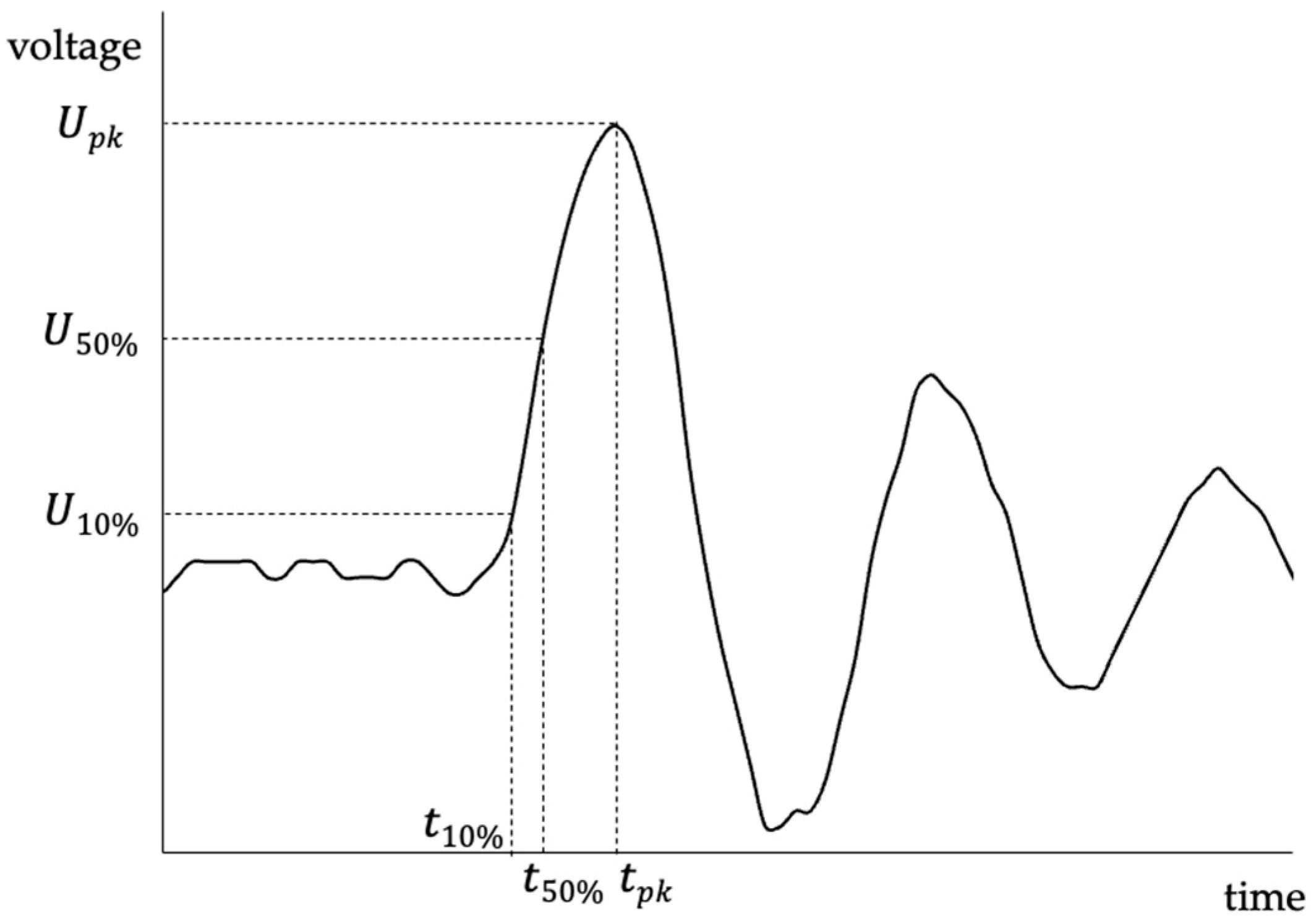
Furthermore, when determining the velocity of traveling waves within a cable based on pulse pairs, the question arises of how to base the measurements with regard to the detected pulses. The two pulses, initial and reflected, each have an approximate origin point, a peak value, a half-value, etc., when observed in the time domain. Additionally, it is not at all certain if establishing the time measurement on different characteristic values of the pulses will yield an equivalent result. These different pulse values and their corresponding time values are illustrated in Figure 1.
There are, therefore, several different estimates of the pulse velocity which may be considered, and it is not a straightforward exercise to determine which of these is the obvious “correct” propagation velocity. Prior research has shown that when pulse detection is based on the pulse onset rather than the peak value, the PD locations are shifted towards the near end of the cable [27]. Some other metrics that can be used to determine the presence and location of a pulse in a time-series measurement involve calculating the derivative of the signal and identifying the time instant corresponding to either the maximum value of the derivative or the last zero value of the derivative prior to the maximum value [28].
In this study, the velocity values are calculated based on the temporal difference between the pulse peaks, the half-value on the rising edge of the pulses, and also the 10% value on the rising edge of the pulses are considered. While these values are somewhat arbitrary, in alternative contexts, these are widely accepted as preferable characteristic values used in the quantification of pulsed and pulse-like phenomena. Equations (4)–(6) describe the different pulse propagation velocities calculated from measurement data. In the subscripts, “1” denotes the original pulse, “2” denotes the reflected pulse, “pk” denotes the peak value, “50%” is the half-value at the rising edge, and “10%” is 10% of the peak value at the rising edge.
The technical implementation of this measurement approach must also consider that the output of PD detection sensors tends to oscillate following the PD pulse, as can be observed in Figure 1. These oscillations can be erroneously interpreted as pulse reflections, especially when a computer algorithm is used to analyze measurement data without appropriate human supervision. In these experiments, care was taken to ensure that the original and reflected pulses were correctly identified.
2. Experimental Setup and Measurements
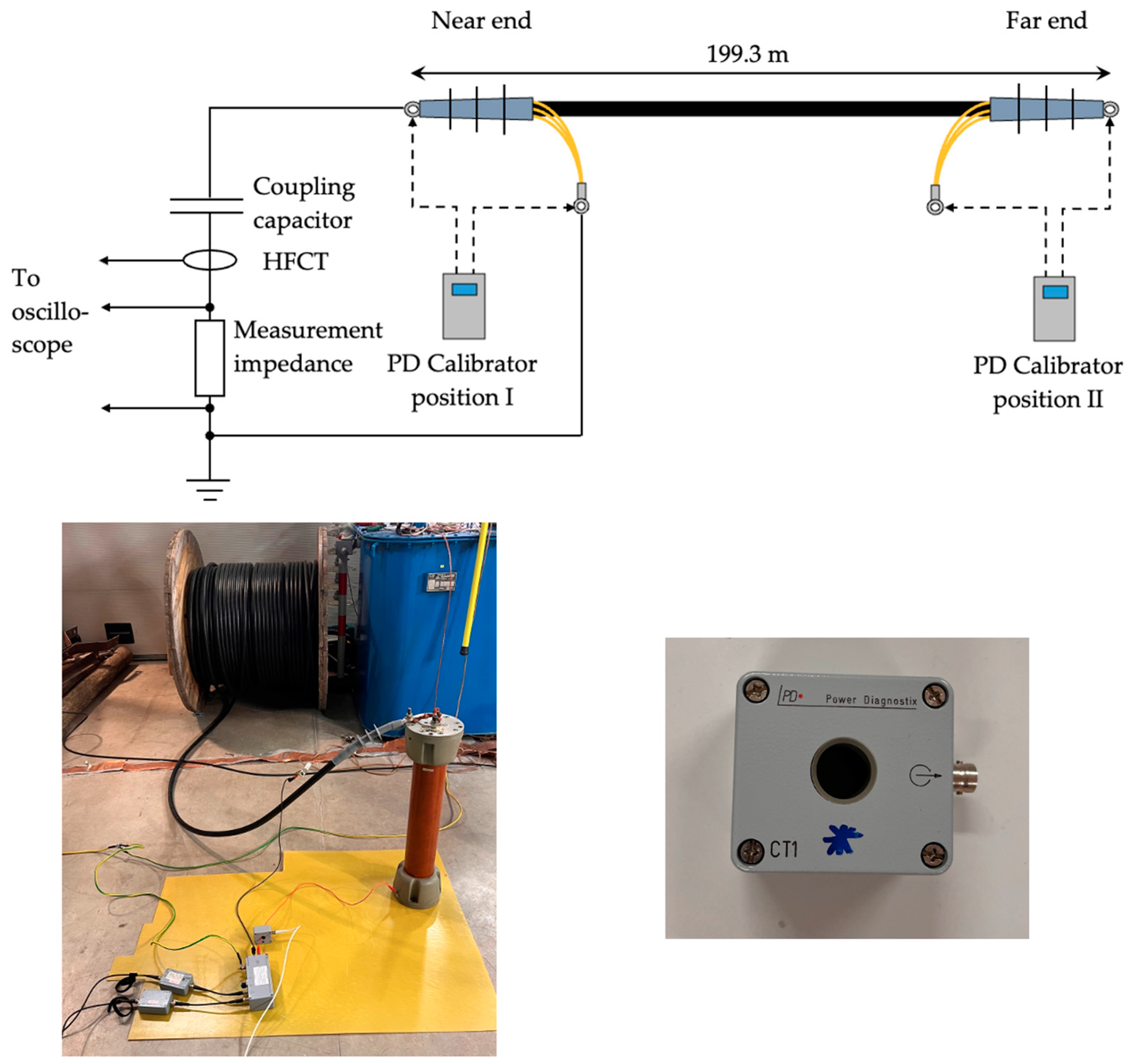
The test setup used in this study included a 199.3 m long 20 kV power cable, in which the pulse propagation velocity was measured. The cable was fitted with terminations at both ends, and the reported length (measured from cable lug to cable lug) is based on the distance markings printed onto the outer sheath. The cable type was HXCMK with a 35 mm2 cross-section copper conductor and a 16 mm2 copper wire screen. The cable was attached to the 1 nF coupling capacitor of an IEC 60270-compliant conventional PD measuring system. An HFCT was also included in the test setup and placed as close as practicable to the quadrupole of the conventional system. The quadrupole also contained the measurement impedance from which the PD signal was captured. This approach was used to minimize the difference in the PD currents measured by each device. The laboratory test setup is depicted in Figure 2.
A PD calibrator was used to inject several pulses with a consistent waveform into the cable. The output of the HFCT, as well as that of the conventional measurement system, was monitored and recorded using a 200 MHz digital storage oscilloscope. The acquisition parameters for each of the measurements were set as follows:
- Sampling rate 2 GS/s;
- Vertical resolution 10-bit;
- Record length 10 kpts (i.e., 5 μs).
The recorded time period was chosen such that it was sufficiently long to capture the initial pulse response from both measurement devices and its first reflection from the opposite cable end while being sufficiently short so as to omit secondary and other subsequent reflections from the measured data. The parameters of the HFCT are as follows:
- Bandwidth (−3 dB): 0.5 MHz to 80 MHz;
- Transfer ratio: 1:10.
The conventional system used was highly adjustable, but in principle, it is a wide-band PD measurement system with a tunable pass-band. In these measurements, the full measurement band from 40 to 800 kHz was used. Additionally, the signal generated from the measured impedance is passed through an amplifier with adjustable gain before being measured; therefore, the measured signal values are substantially higher for the conventional PD system (in the range of volts) than in the case of the HFCT, which outputs peak signal values in the millivolt range.
In order to obtain a more comprehensive overview of the statistical variability of the velocity measurement, the data analysis was performed on a series of 1000 pulses gathered during each individual experiment, with the other parameters kept constant. The pulses were injected into the cable at a rate of 100 per second, and the oscilloscope recorded all of these pulse responses in a segmented measurement mode, which were subsequently analyzed using computer software to calculate the propagation velocity. Because the temperature slightly affects propagation velocity, the tests were performed in indoor conditions at a consistent ambient temperature of 21 °C. The testing itself did not impart any substantial thermal effect on the cable; therefore, the temperature variability is practically excluded as a source of measurement uncertainty.
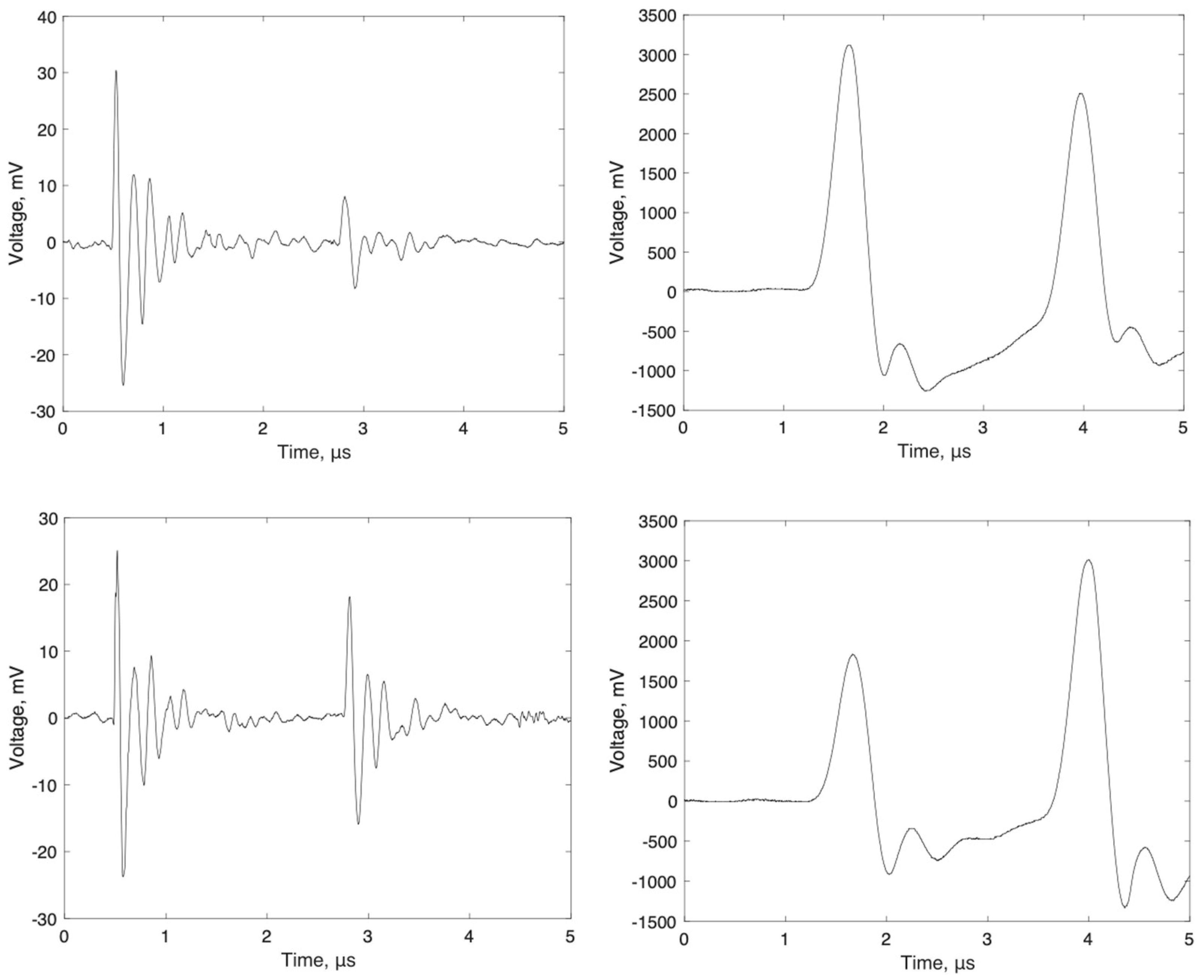
A peculiar phenomenon was observed when injecting the pulses into the cable at the near end with regard to the measurement equipment. As can be seen in Figure 3, the reflected pulse appears to have a higher amplitude than the initial pulse when measured using the conventional system. This observation is highly counterintuitive, as it appears to defy the law of energy conservation, at least when based on initial impressions. It can also be observed that although the reflected pulse response amplitude is clearly lower in the case of the HFCT, regardless of whether the pulse is injected at the near or far end of the cable, the reflected pulse response is notably smaller in the case of the far-end pulse injection. When comparing the response measured when the pulse is injected at the far end of the cable, the waveform seems to be as predicted by the theory, i.e., the reflected pulse presents with a lower peak value than the original pulse. This paradox can be explained based on the following reasoning.
The cable’s characteristic impedance is lower than that of the external circuit connected to the cable. In the case of the near-end pulse injection, where the pulse is generated at the interface separating the two media with unequal characteristic impedances, a larger current is generated in the cable as opposed to the measurement circuit connected to the cable. The measurement circuit then records the response to this initial pulse. Now, it is necessary to consider what happens to the pulse that begins to travel down the cable to the opposite open end of the cable. It is affected by attenuation and dispersion, as described previously. As it reaches the far end of the cable, a complete reflection of the pulse occurs. This reflected pulse continues to propagate towards the near end and reaches the interface between the measurement equipment and the cable. At this discontinuity, a portion of the pulse is reflected back into the cable, while the remaining portion propagates out from the cable and into the measurement circuit, where it is recorded as the “reflected” pulse. It can be shown that if the disparity between the characteristic impedances is sufficiently high and the attenuation in the cable sufficiently low (i.e., the cable is short enough and does not degrade the pulse excessively), the reflected pulse can be measured to have a higher response amplitude than the initial pulse.
In the other case, i.e., when the pulse is generated at the far end of the cable, the entire pulse energy is injected into the cable as there is only one possible direction for its propagation from the injection point. Due to the lossy nature of the cable, every time the pulse reaches the near end of the cable after reflecting from the open opposite end of the cable, the peak values of the measured responses will decrease in comparison to the preceding peak.
In the case of the HFCT, however, it can be seen that there is a smaller difference between the original and reflected pulses when the pulse is injected at the near end of the cable, as opposed to the far end of the cable. Yet, the reflected pulse produces a lower response amplitude in both cases. This can be explained by the fact that the HFCT responds to higher frequencies than the commercial PD measurement system. Because higher frequencies are attenuated more strongly, the response to the reflected pulse will remain lower in both cases, given the conditions under which this experiment was performed.
3. Results
Some examples of the pulse waveforms that were measured using both the HFCT and the conventional IEC 60270-compliant system are presented in Figure 3. The effect described in the previous section is visible in the case of the conventional system. Another difference between the two measurement methodologies can also be observed, as it also pertains to the pulse resolution time of either device. In the case of the HFCT, the oscillations from the initial pulse have almost fully subsided by the time the reflected pulse reaches the measurement device. This results in a crisp response and two easily distinguishable pulse responses in the waveform. In the case of the conventional system, however, the detection circuit has not yet fully recovered from the initial pulse and has therefore not settled to a near-zero steady state when the reflected pulse reaches the sensor. Although the responses to the two pulses are easily distinguishable, this phenomenon affects the test results somewhat and, therefore, caution in interpreting the results is warranted. As the noise level is sufficiently low in these measurements, no denoising techniques were applied prior to subjecting the data to further processing.
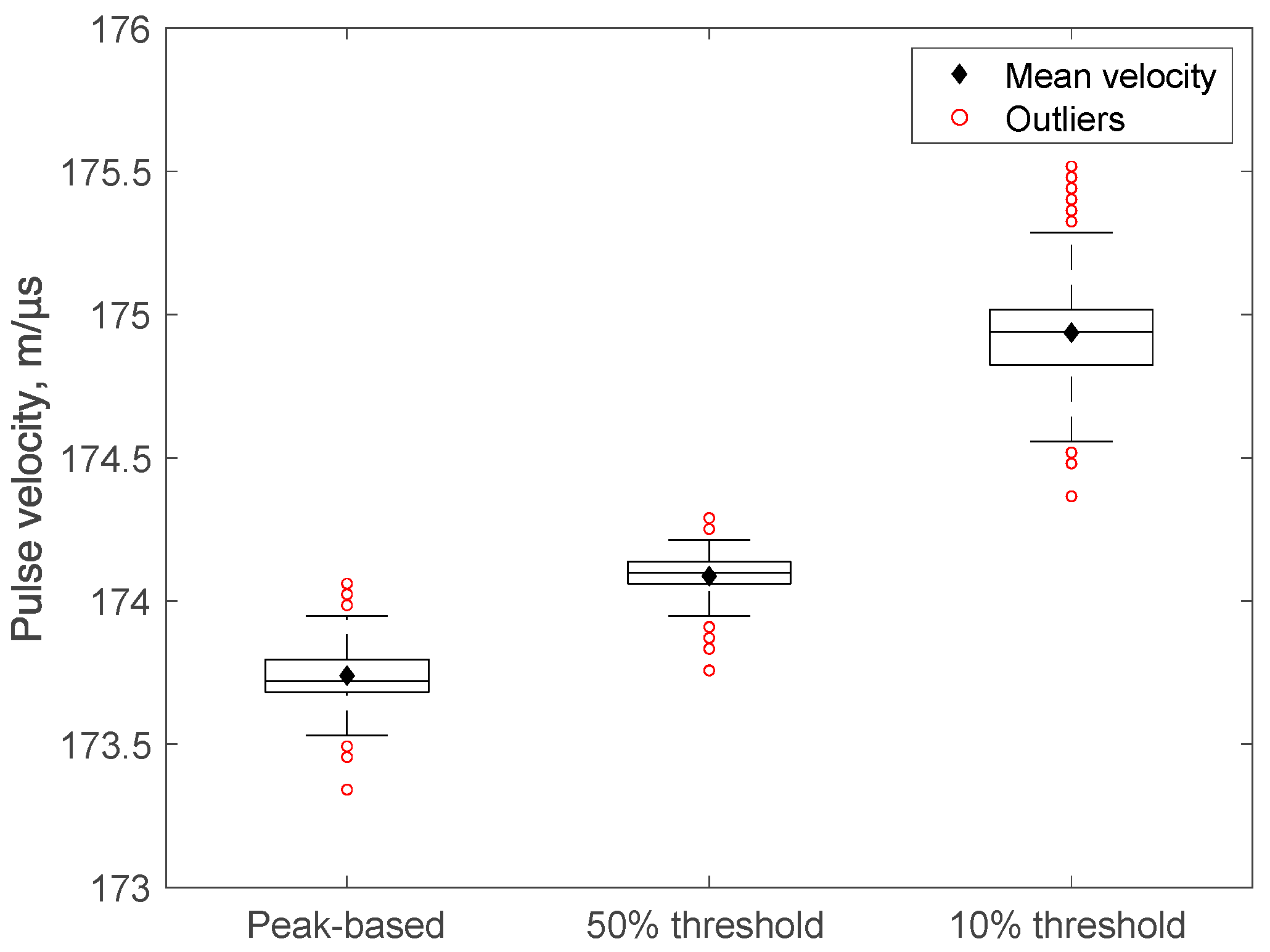
The calculated pulse velocity results are comprehensively presented in Figure 4, Figure 5, Figure 6, Figure 7, Figure 8, Figure 9, Figure 10 and Figure 11, as both box-and-whisker plots and histograms, to provide a better overview of the distribution of the individual measurement results. Pulse velocities based on all the aforementioned characteristics are presented, i.e., peak-value-based, half-value-based, and 10% threshold-value-based. The values were individually calculated for both the original and reflected pulses. All these data were gathered by injecting 1 nC pulses into the cable using the pulse calibrator. Both the near- and far-end injection, as well as both the HFCT and IEC 60270-compliant measurement devices, were used to diversify the range of parameters investigated. After the initial testing, the 1 nC charge generated by a pulse calibrator was chosen to produce consistent pulses for performing the measurements.
In the box-and-whisker plots, the box represents the interquartile range, i.e., the lower and upper edges correspond to the 25th and 75th percentile, respectively. The “whisker” lengths are chosen as 1.5 times the interquartile range, with any outliers separately plotted using a red circle as the marker. The median, i.e., the 50th percentile of the distribution, is denoted by the line in the middle part of the “box”. In the velocity histograms, the bin width is chosen as 0.1 m/μs across all the figures for easier comparison between the different measurement configurations. The histograms are supplemented with line sections, indicating one standard deviation (SD) on either side of the calculated mean velocity. The velocity measurement results are summarized in Table 1.
4. Analysis and Discussion
Some notable observations can be made from these data. First of all, when comparing the two measurement systems, it is clear that the velocity measured using the HFCT is greater than the velocity measured using the IEC 60270-compliant conventional system. The velocities measured using the HFCT are approximately 174 m/μs, whereas those measured using the conventional system are approximately 172 m/μs. This can be explained by the fact that the higher frequencies do indeed propagate faster in the cable, as many researchers have previously observed, and the bandwidth of the measurement devices is in a higher range for the HFCT compared to the conventional system.
Secondly, the calculated velocity is dependent on whether the calibration pulse is injected at the near or far end of the cable. With the HFCT, the measured velocity was higher when the pulse was injected at the far end of the cable, regardless of which pulse characteristic the velocity was based on. In the case of the conventional system, this was also observed for the peak-based velocity but not for the 50% or 10% threshold values. As mentioned previously, the conventional system had some difficulty in fully resolving the two subsequent pulses due to their short interval. This introduces a notable bias in determining 50% and 10% threshold values. However, the location of the peak of the reflected pulse response was not significantly affected. As mentioned previously, the drawback, in this case, was that the sensor output could not restabilize over the short time period between the original and reflected pulses.
Thirdly, it appears that the variability of the measurement results is notably larger in the case of the conventional system, which is observed in almost all the measurements. The larger variability can mostly be explained by the nature of the response of each system. In the case of the HFCT, the response is much more dynamic, as is evident from Figure 3, whereas the response pulse produced by the conventional system is substantially wider. This makes the system more susceptible to random interferences and subsequently produces a wider distribution in the calculated pulse velocity.
Fourthly, the variance is substantially smaller in case the velocity is calculated based on the half-value of the pulse response when compared to either the peak value or the 10% threshold. This can be observed across all the measurements performed with both systems. The smaller variance can be explained by the fact that the rate of change in the signal is largest around the 50% peak threshold. The rapid change also confers the highest degree of immunity against random disturbances in this part of the signal, providing the most consistent pulse velocity values.
Fifthly, the velocity of propagation is dependent on which characteristic of the pulse it is based on. In the case of the HFCT, the calculated propagation velocity increases in the sequence: the peak value, 50% value, and 10% value. This can be explained by the aforementioned distortion in the pulse waveform due to attenuation and dispersion. The relative amount of delay the waveform experiences is greater at the peak value. Therefore, the time delay associated with the peak values will also be greater, resulting in a lower calculated propagation velocity.
It should also be noted that, across all the measurement results, the median velocity is approximately equal to the mean velocity, which is to be expected. It indicates that the velocity distribution is relatively symmetrical, as can also be observed from the results (Figure 4, Figure 5, Figure 6, Figure 7, Figure 8, Figure 9, Figure 10 and Figure 11). The random errors affecting the measurements appear to follow an approximately normal distribution.
These results also indicate that the propagation velocity can change substantially between subsequent measurements. When relying on the measurements based on pulse peaks, there is a notable probability of measuring a value close to 170 m/μs or 172 m/μs, whereas the most likely value is around 171 m/μs (based on Figure 9). Therefore, a significant risk exists to the accuracy of the velocity assessment when relying on only one measurement; at least some repeat measurements should be performed prior to using the propagation velocity in the analysis of PD measurements. In environments with higher levels of noise, the variability across measurements is likely to be even more prominent. It would also be prudent to consider preferentially using the propagation velocity based on the pulse half-value due to its lower variability and a greater degree of immunity to the stochastic effects.
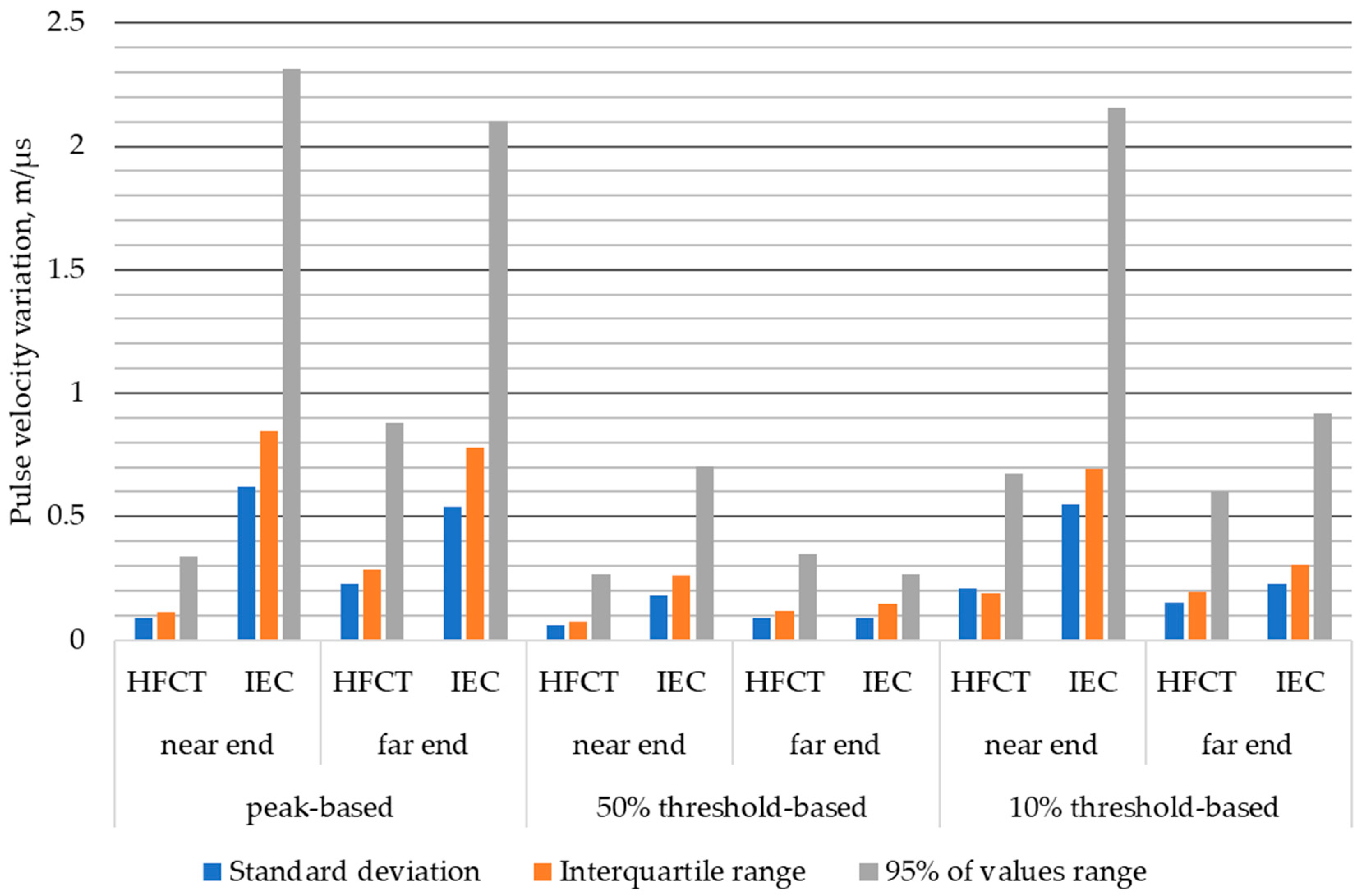
The variability of the pulse propagation velocity measurements is comprehensively illustrated in Figure 12. In the figure, the 95% of values range considers the middle 95% of all measurement results, i.e., it is the inter-percentile range between the 2.5th and the 97.5th percentile. It is apparent that the variability metrics of the half-value-based approach to velocity measurement are substantially smaller than in the case of the other two approaches.
The higher variability between measurements performed using the conventional system is evident in most of the studied cases, which is independent of the variability metric considered. The IEC method appears more susceptible to measurement noise when the calibration pulse is injected near the cable’s end, as the variability metrics for near-end injection are higher in all three cases. The HFCT, alternatively, appears to be more susceptible to measurement noise when the pulse is injected at the far end of the cable, as can be seen in the case of the peak- and half-value-based measurements. In the case of the 10% threshold-based velocity measurement, the difference caused by the choice of the injection site is modest.
It is also noteworthy that while the IEC 60270-compliant system produces much larger variance in most cases, the variability metrics of the measurements performed using the two measurement systems are almost identical when using the 50% value and when the pulse is injected at the far end of the cable. In fact, when considering the 95% values range, the variability of the conventional system measurements is lower than those of the HFCT, which does not occur in any other case. This implies that the commonly held belief that using an HFCT for PD detection in power cables is superior can also be context-dependent, and the conventional IEC 60270 system is not necessarily inferior to an HFCT under some specific circumstances.
In order to illustrate the significance of these differences in velocity measurement, it is appropriate to consider a cable 1 km in length. When there is a PD source close to the near end of the cable, the difference in the apparent location of the source, when determined via TDR using the velocities characteristic of the HFCT and conventional measurement, is approximately 15 m. This is in the order of 1% of the cable length, which has substantial practical implications if the PD source is to be located and repaired. This illustrates why calibration is always necessary prior to the PD measurement and that attributing a single-pulse velocity parameter to any power cable is problematic. Determining PD source locations using the same method utilized for velocity measurement should yield more accurate results.
When considering the variability between measurements, it is appropriate to consider the example with the conventional system, where the values of measured velocity are spread around 2 m/μs. This would yield a location difference of approximately 10 m, which is also in the order of 1% of the cable length. The variability of the HFCT measurements is spread around 1 m/μs, corresponding to a spatial difference of approximately 5 m, which is somewhat better than the conventional system. However, when considering a situation where the velocity is based on the 50% peak threshold value, the calculated location variabilities are reduced to 4 m for the conventional system and down to 1 m for the HFCT. This is only 0.1% of the cable length, which constitutes a significant improvement in location accuracy.
The cable used in this study did not have any joints, which are uncharacteristic of the longer cables operating in the grid. Joints constitute discontinuities where the characteristic impedance of the cable system changes and, therefore, some of the pulse energy is reflected at the joints. This will have an impact on the waveform of propagating signals, with the magnitude of the effect depending on the cable and joint combination. It is likely that results similar to those presented in this study are observed in cables with joints; however, further investigations will have to determine the validity of this conjecture.
Another aspect of the PD measurement is the application of signal processing techniques to denoise the measured signal and improve the identification of PD pulses. While the signals recorded in this study were sufficiently unaffected by sources of interference so as not to require denoising, measurements made in on-site conditions can often be affected by substantial levels of electromagnetic noise. As there are several denoising methods available, investigating how denoising affects the signal waveform and how this can impact the determination of the pulse velocity based on the methods described in this paper can be a possible direction for further research.
In summary, this work presents an in-depth study of the behavior and impact of the measurement approaches on the accuracy of the propagation velocity, and future work can include attempts to reproduce these results with various cable systems. The cable used in this experiment was rather short, approximately 200 m in length, and it would be useful to determine whether concordant data are gathered when measuring the propagation velocity in cables of around 1 km in length or longer. Investigating what effect joints and signal denoising techniques have on the determination of pulse velocity using the methodologies presented in this paper is another prospective direction for further research. Additionally, further work to quantify the effect these different approaches to pulse propagation velocity have on an actual PD source location is the next logical step to determine the real-world impact of propagation velocity variation and the measurement errors involved. Approaches to compensate for the systemic errors intrinsic to the measurement process can also be a possible direction for further inquiry.
5. Conclusions
The results of this investigation indicate that:
- The bandwidth of the measurement system influences the determined propagation velocity. The pulse propagation velocity, measured using a high-frequency current transformer (HFCT), which has a higher measurement bandwidth than an IEC 60270-compliant conventional measurement system, is also higher.
- The propagation velocity, measured using an HFCT, has a smaller variability between the individual measurements in most cases, providing a less statistically variable estimate of the pulse velocity. In this regard, the HFCT is generally superior to the conventional measurement system for PD measurements in power cables.
- Basing the velocity measurement on the half-value time instants at the rising edge of both the incident and reflected pulses will provide a more consistent estimate of propagation velocity (i.e., lower statistical variability) when compared to either the peak value times or those crossing a lower threshold close to the pulse origin, e.g., 10% of the peak at the rising edge. Therefore, the half-values at the rising edge of both the original and reflected pulses should be the preferred reference points for determining the pulse velocity.
- Care should be taken to check whether the reflected pulse reaches the measurement sensor while it recovers from the incident pulse or has already reached a steady state. If the sensor output has not stabilized, using values other than the peak value to determine the pulse velocity will yield an erroneous or highly biased result.
Author Contributions
Conceptualization, I.K.; data curation, I.K.; formal analysis, I.K., M.S., M.C., M.P., I.P. and P.T.; funding acquisition, M.S.; investigation, I.K.; methodology, I.K.; project administration, M.S.; software, I.K. and M.P.; validation, M.S., M.C., M.P., I.P. and P.T; visualization, I.K.; writing—original draft preparation, I.K.; writing—review and editing, M.S., M.C., M.P., I.P. and P.T. All authors have read and agreed to the published version of the manuscript.
Funding
This work was supported by the Estonian Research Council under grant PSG 632.
Data Availability Statement
The data supporting the research of this paper are available upon request from the corresponding author.
Conflicts of Interest
The authors declare no conflict of interest. The funders had no role in the design of the study; in the collection, analyses, or interpretation of data; in the writing of the manuscript; or in the decision to publish the results.
References
- IEC 60270:2000/A1:2015; High-Voltage Test Techniques—Partial Discharge Measurements. IEC: Geneva, Switzerland, 2015.
- Yaacob, M.M.; Alsaedi, M.A.; Rashed, J.R.; Dakhil, A.M.; Atyah, S.F. Review on Partial Discharge Detection Techniques Related to High Voltage Power Equipment Using Different Sensors. Photonic Sens. 2014, 4, 325–337. [Google Scholar] [CrossRef] [Green Version]
- Montanari, G.C. Partial Discharge Detection in Medium Voltage and High Voltage Cables: Maximum Distance for Detection, Length of Cable, and Some Answers. IEEE Electr. Insul. Mag. 2016, 32, 41–46. [Google Scholar] [CrossRef]
- Wild, M.; Tenbohlen, S.; Gulski, E.; Jongen, R.; de Vries, F. Practical Aspects of PD Localization for Long Length Power Cables. In Proceedings of the 2013 IEEE Electrical Insulation Conference (EIC), Ottawa, ON, Canada, 2–5 June 2013; pp. 499–503. [Google Scholar]
- van der Wielen, P.C.J.M.; Veen, J.; Wouters, P.A.A.F.; Steennis, E.F. On-Line Partial Discharge Detection of MV Cables with Defect Localisation (PDOL) Based on Two Time Synchronised Sensors. In Proceedings of the CIRED 2005—18th International Conference and Exhibition on Electricity Distribution, Turin, Italy, 6–9 June 2005; pp. 1–5. [Google Scholar]
- Mohamed, F.P.; Siew, W.H.; Soraghan, J.J.; Strachan, S.M.; McWilliam, J. Partial Discharge Location in Power Cables Using a Double Ended Method Based on Time Triggering with GPS. IEEE Trans. Dielectr. Electr. Insul. 2013, 20, 2212–2221. [Google Scholar] [CrossRef]
- Wagenaars, P.; Wouters, P.A.A.F.; van der Wielen, P.C.J.M.; Steennis, E.F. Accurate Estimation of the Time-of-Arrival of Partial Discharge Pulses in Cable Systems in Service. IEEE Trans. Dielectr. Electr. Insul. 2008, 15, 1190–1199. [Google Scholar] [CrossRef] [Green Version]
- IEC 60885-3; Electrical Test Methods for Electric Cables—Part 3: Test Methods for Partial Discharge Measurements on Lengths of Extruded Power Cables. IEC: Geneva, Switzerland, 2015.
- Mugala, G. Influence of the Semi-Conducting Screens on the Wave Propagation Characteristics of Medium Voltage Extruded Cables. Licenciate Thesis, Royal Institute of Technology, Stockholm, Sweden, 2003. [Google Scholar]
- Shafiq, M.; Kütt, L.; Mahmood, F.; Hussain, G.A.; Lehtonen, M. An Improved Technique to Determine the Wave Propagation Velocity of Medium Voltage Cables for PD Diagnostics. In Proceedings of the 2013 12th International Conference on Environment and Electrical Engineering, Wroclaw, Poland, 5–8 May 2013; pp. 539–544. [Google Scholar]
- Dubickas, V.; Edin, H. On-Line Time Domain Reflectometry Measurements of Temperature Variations of an XLPE Power Cable. In Proceedings of the 2006 IEEE Conference on Electrical Insulation and Dielectric Phenomena, Kansas City, MO, USA, 15–18 October 2006; pp. 47–50. [Google Scholar]
- Mugala, G.; Eriksson, R.; Pettersson, P. Dependence of XLPE Insulated Power Cable Wave Propagation Characteristics on Design Parameters. IEEE Trans. Dielectr. Electr. Insul. 2007, 14, 393–399. [Google Scholar] [CrossRef]
- Kreuger, F.H.; Wezelenburg, M.G.; Wiemer, A.G.; Sonneveld, W.A. Partial Discharge. XVIII. Errors in the Location of Partial Discharges in High Voltage Solid Dielectric Cables. IEEE Electr. Insul. Mag. 1993, 9, 15–22. [Google Scholar] [CrossRef] [Green Version]
- Boggs, S.; Pathak, A.; Walker, P. Partial Discharge. XXII. High Frequency Attenuation in Shielded Solid Dielectric Power Cable and Implications Thereof for PD Location. IEEE Electr. Insul. Mag. 1996, 12, 9–16. [Google Scholar] [CrossRef]
- O, H.N.J. Propagation of High Frequency Partial Discharge Signal in Power Cables. PhD Thesis, University of New South Wales, Sydney, Australia, 2009. [Google Scholar]
- Li, Y.; Wouters, P.A.A.F.; Wagenaars, P.; van der Wielen, P.C.J.M.; Steennis, E.F. Temperature Dependent Signal Propagation Velocity: Possible Indicator for Mv Cable Dynamic Rating. IEEE Trans. Dielectr. Electr. Insul. 2015, 22, 665–672. [Google Scholar] [CrossRef]
- Shafiq, M.; Kiitam, I.; Taklaja, P.; Kütt, L.; Kauhaniemi, K.; Palu, I. Identification and Location of PD Defects in Medium Voltage Underground Power Cables Using High Frequency Current Transformer. IEEE Access 2019, 7, 103608–103618. [Google Scholar] [CrossRef]
- Paophan, B.; Kunakorn, A.; Yutthagowith, P.; Pumyoy, S. Study of A Partial Discharge Location Technique for Power Cables Using High Frequency Current Transducer. In Proceedings of the 2018 Australasian Universities Power Engineering Conference (AUPEC), Auckland, New Zealand, 27−30 November 2018; pp. 1–4. [Google Scholar]
- Shafiq, M.; Robles, G.; Hussain, G.; Kauhaniemi, K.; Lehtonen, M. Identification and Location of Partial Discharge Defects in Medium Voltage AC Cables. In Proceedings of the Nordic Insulation Symposium, Tampere, Finland, 5 August 2019; pp. 22–27. [Google Scholar]
- Robles, G.; Shafiq, M.; Martínez-Tarifa, J.M. Multiple Partial Discharge Source Localization in Power Cables Through Power Spectral Separation and Time-Domain Reflectometry. IEEE Trans. Instrum. Meas. 2019, 68, 4703–4711. [Google Scholar] [CrossRef]
- Ragusa, A.; Sasse, H.G.; Duffy, A. On-Line Partial Discharge Localization in Power Cables Based on Electromagnetic Time Reversal Theory—Numerical Validation. IEEE Trans. Power Deliv. 2022, 37, 2911–2920. [Google Scholar] [CrossRef]
- Ragusa, A.; Sasse, H.; Duffy, A. Practical Evaluation of Electromagnetic Time Reversal to Locate Partial Discharges on Power Networks in the Presence of Noise. In Proceedings of the 2022 IEEE International Symposium on Electromagnetic Compatibility & Signal/Power Integrity (EMCSI), Spokane, WA, USA, 1–5 August 2022; pp. 635–640. [Google Scholar]
- Mahdipour, M.; Akbari, A.; Werle, P.; Borsi, H. Partial Discharge Localization on Power Cables Using On-Line Transfer Function. IEEE Trans. Power Deliv. 2019, 34, 1490–1498. [Google Scholar] [CrossRef]
- Mardiana, R.; Su, C.Q. Partial Discharge Location in Power Cables Using a Phase Difference Method. IEEE Trans. Dielectr. Electr. Insul. 2010, 17, 1738–1746. [Google Scholar] [CrossRef]
- Fantoni, P.F. Condition Monitoring of Electrical Cables Using Line Resonance Analysis (LIRA). In Proceedings of the 9th International Conference on Insulated Power Cables (Jicable’15), Versailles, France, 21–25 June 2015; pp. 1–5. [Google Scholar]
- Mahdipour, M.; Akbari, A.; Werle, P. Cable Joints Effect in Partial Discharge Signal Propagation. In Proceedings of the 20th International Symposium on High Voltage Engineering (ISH), Buenos Aires, Argentina, 28 August–1 September 2017; pp. 1–6. [Google Scholar]
- Herold, C.; Leibfried, T. Signal Processing Tools for Evaluation of Partial Discharge Measurement Data of Power Cables. In Proceedings of the 2008 Annual Report Conference on Electrical Insulation and Dielectric Phenomena, Quebec, QC, Canada, 26–29 October 2008; pp. 525–527. [Google Scholar]
- Giaquinto, N.; D’Aucelli, G.M.; De Benedetto, E.; Cannazza, G.; Cataldo, A.; Piuzzi, E.; Masciullo, A. Accuracy Analysis in the Estimation of ToF of TDR Signals. In Proceedings of the 2015 IEEE International Instrumentation and Measurement Technology Conference (I2MTC) Proceedings, Pisa, Italy, 11–14 May 2015; pp. 187–192. [Google Scholar]
Figure 1.
Peak, 50% threshold and 10% threshold values of a PD detector response and their corresponding time instants.
Figure 1.
Peak, 50% threshold and 10% threshold values of a PD detector response and their corresponding time instants.

Figure 2.
Test setup for measuring pulse propagation velocity in a power cable (top); test setup in the laboratory (bottom left); high-frequency current transformer used in experiments (bottom right).
Figure 2.
Test setup for measuring pulse propagation velocity in a power cable (top); test setup in the laboratory (bottom left); high-frequency current transformer used in experiments (bottom right).

Figure 3.
Examples of measured responses to pulses injected at the far end of the cable (top row) and the near end of the cable (bottom row). (Left): HFCT; (Right): IEC 60270−compliant conventional system.
Figure 3.
Examples of measured responses to pulses injected at the far end of the cable (top row) and the near end of the cable (bottom row). (Left): HFCT; (Right): IEC 60270−compliant conventional system.

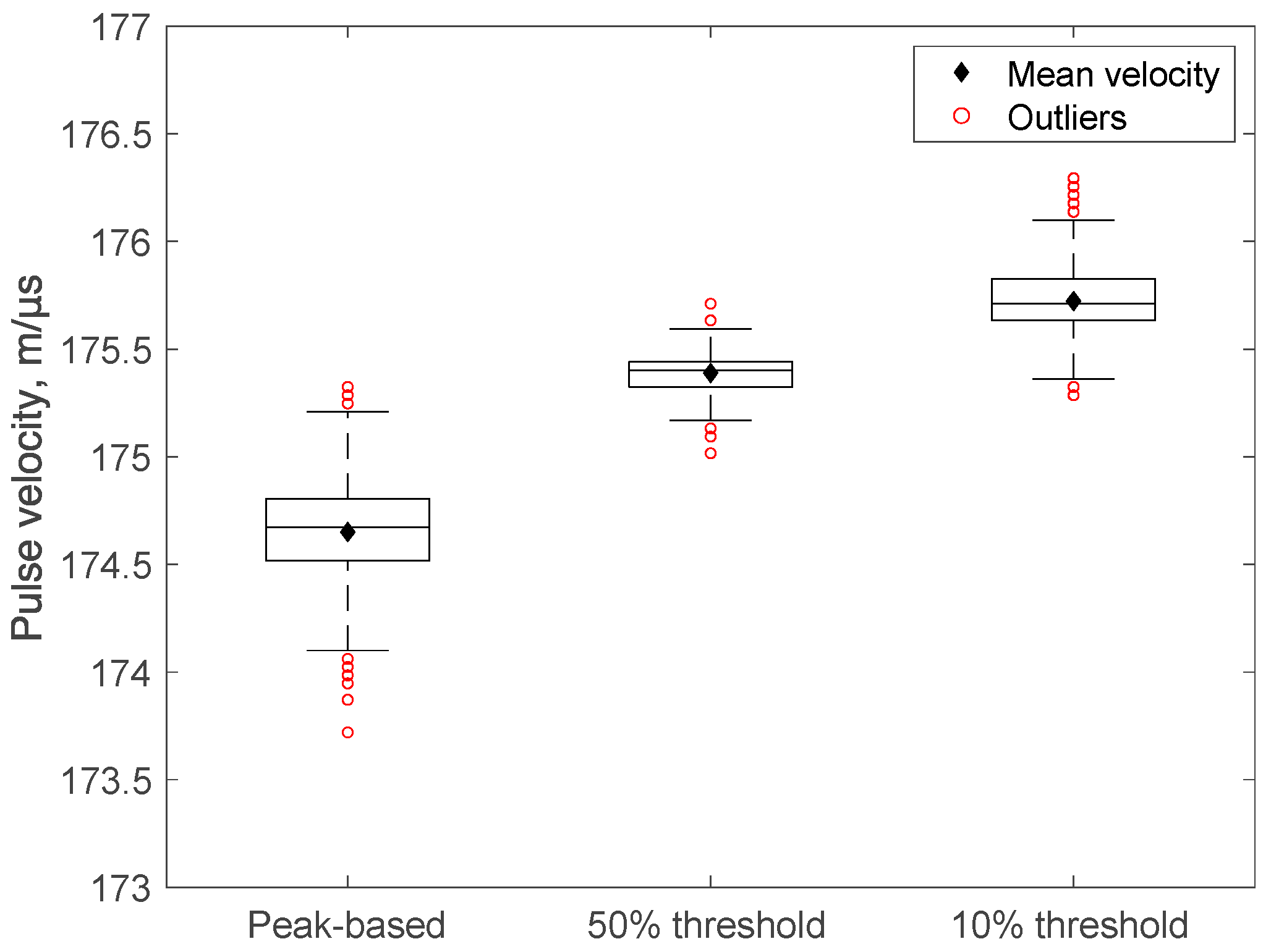
Figure 4.
Pulse velocity box plots for 1 nC pulse injected near the cable’s end, measured using HFCT.
Figure 4.
Pulse velocity box plots for 1 nC pulse injected near the cable’s end, measured using HFCT.

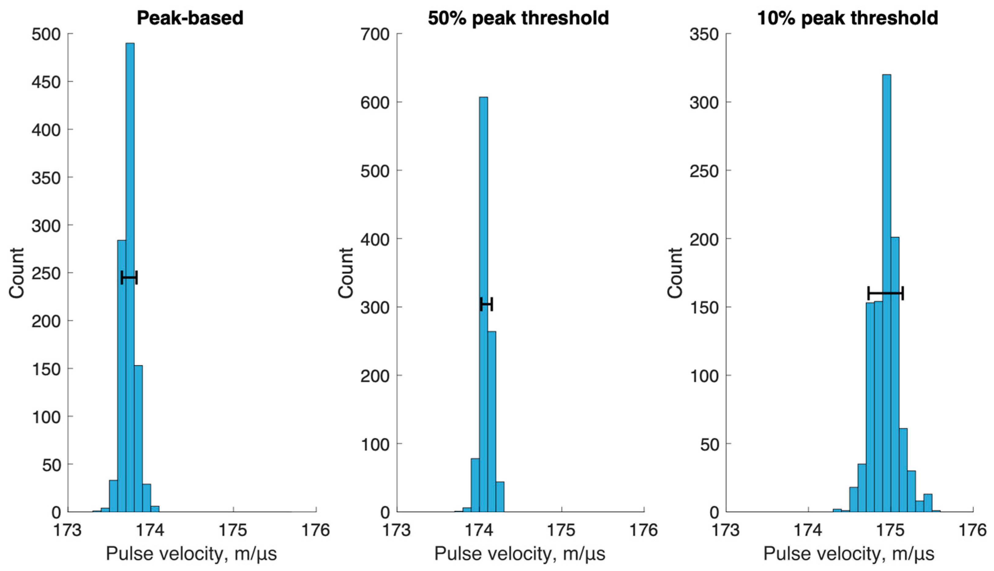
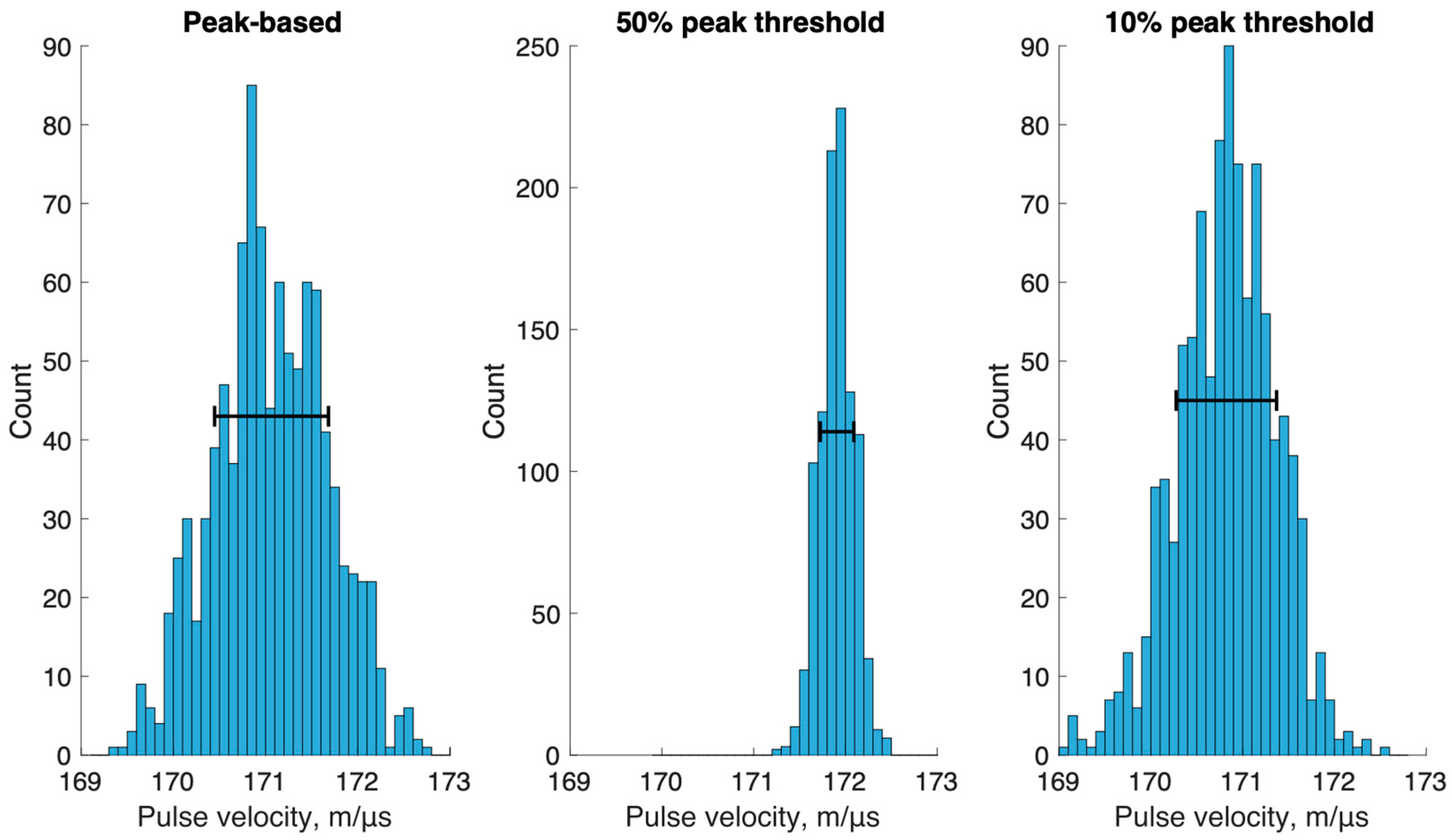
Figure 5.
Pulse velocity histograms for 1 nC pulses (1000 total) injected near the cable’s end, including SD around the mean, measured using HFCT.
Figure 5.
Pulse velocity histograms for 1 nC pulses (1000 total) injected near the cable’s end, including SD around the mean, measured using HFCT.

Figure 6.
Pulse velocity box plots for 1 nC pulse injected at the far end of the cable, measured using HFCT.
Figure 6.
Pulse velocity box plots for 1 nC pulse injected at the far end of the cable, measured using HFCT.

Figure 7.
Pulse velocity histograms for 1 nC pulses (1000 total) injected at the far end of the cable, including SD around the mean, measured using HFCT.
Figure 7.
Pulse velocity histograms for 1 nC pulses (1000 total) injected at the far end of the cable, including SD around the mean, measured using HFCT.

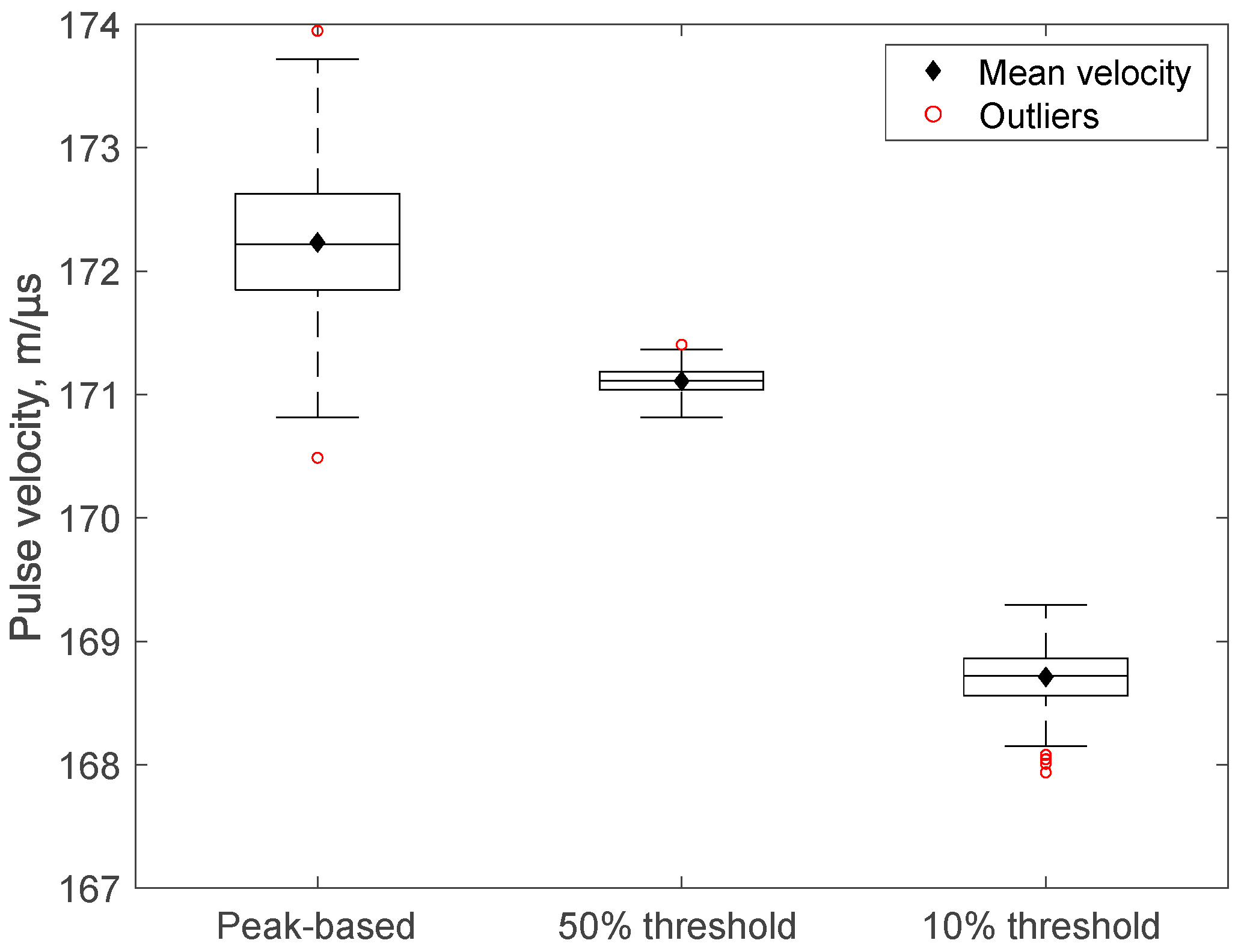
Figure 8.
Pulse velocity box plots for 1 nC pulse injected near the cable’s end, measured using the IEC 60270-compliant system.
Figure 8.
Pulse velocity box plots for 1 nC pulse injected near the cable’s end, measured using the IEC 60270-compliant system.

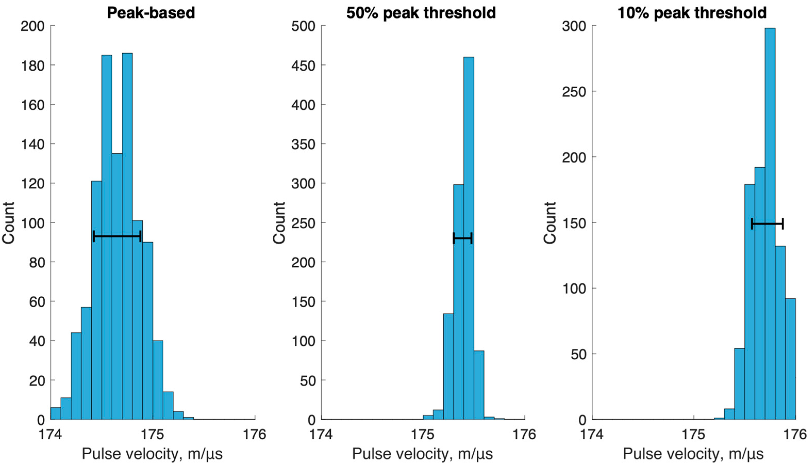
Figure 9.
Pulse velocity histograms for 1 nC pulses (1000 total) injected near the cable’s end, including SD around the mean, measured using the IEC 60270-compliant system.
Figure 9.
Pulse velocity histograms for 1 nC pulses (1000 total) injected near the cable’s end, including SD around the mean, measured using the IEC 60270-compliant system.

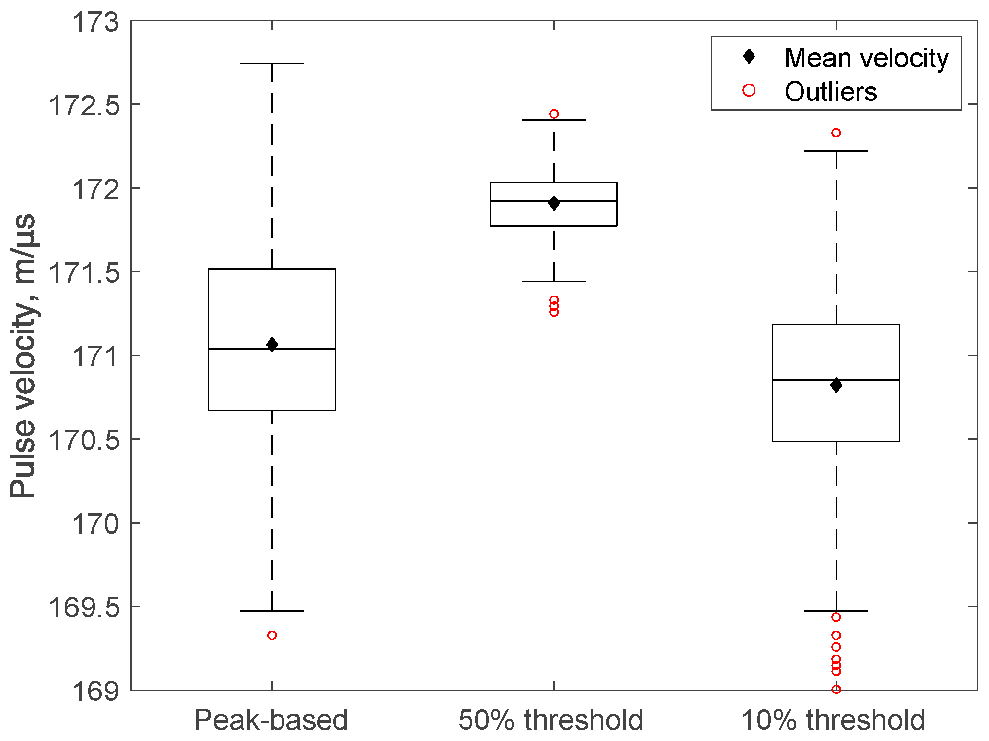
Figure 10.
Pulse velocity box plots for 1 nC pulse injected at the far end of the cable, measured using the IEC 60270-compliant system.
Figure 10.
Pulse velocity box plots for 1 nC pulse injected at the far end of the cable, measured using the IEC 60270-compliant system.

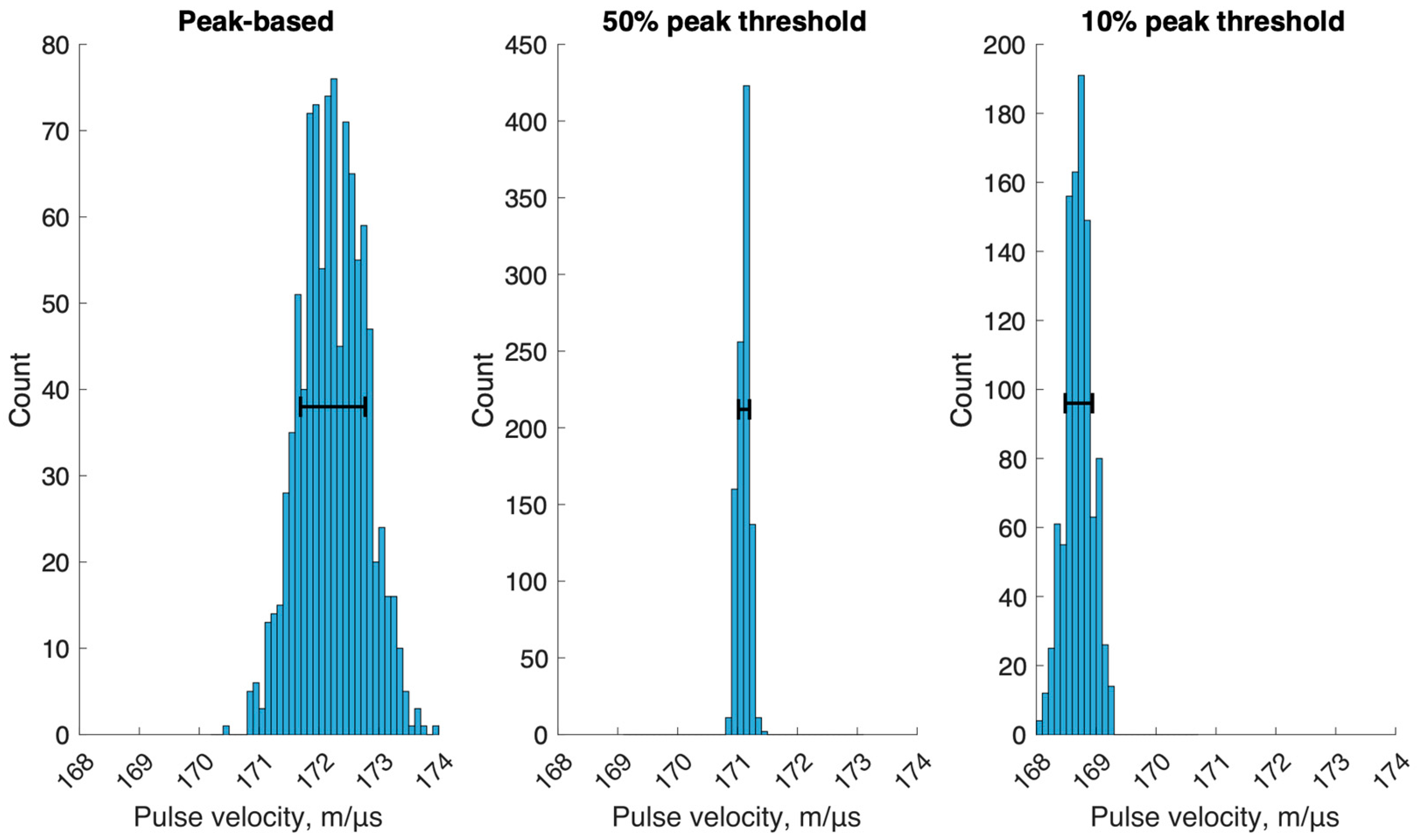
Figure 11.
Pulse velocity histograms for 1 nC pulses (1000 total) injected at the far end of the cable, including SD around the mean, measured using the IEC 60270-compliant system.
Figure 11.
Pulse velocity histograms for 1 nC pulses (1000 total) injected at the far end of the cable, including SD around the mean, measured using the IEC 60270-compliant system.

Figure 12.
Comparison of pulse velocity variation metrics determined using different reference points for velocity measurement, expressed in terms of SD, interquartile range, and 95% of values range, based on 1000 velocity measurements performed for each case.
Figure 12.
Comparison of pulse velocity variation metrics determined using different reference points for velocity measurement, expressed in terms of SD, interquartile range, and 95% of values range, based on 1000 velocity measurements performed for each case.


Table 1.
Summary of pulse propagation velocity measurement results based on different pulse characteristics, including deviation between mean value compared to peak-based measurement.
Table 1.
Summary of pulse propagation velocity measurement results based on different pulse characteristics, including deviation between mean value compared to peak-based measurement.
| Measurement | Mean Velocity (Peak-Based) ± SD, m/μs | Mean Velocity (50%-Based) ± SD, m/μs | Mean Velocity (10%-Based) ± SD, m/μs |
|---|---|---|---|
| High-frequency current transformer | |||
| 1 nC, near end | 173.74 ± 0.09 | 174.09 ± 0.06 (∆ = +0.35) | 174.94 ± 0.21 (∆ = +1.20) |
| 1 nC, far end | 174.65 ± 0.23 | 175.39 ± 0.09 (∆ = +0.74) | 175.72 ± 0.15 (∆ = +1.07) |
| IEC 60270-compliant conventional system | |||
| 1 nC, near end | 171.06 ± 0.62 | 171.91 ± 0.18 (∆ = +0.84) | 170.82 ± 0.55 (∆ = −0.24) |
| 1 nC, far end | 172.23 ± 0.54 | 171.11 ± 0.09 (∆ = −1.12) | 168.71 ± 0.23 (∆ = −3.52) |
| Difference between mean velocities measured using both systems | |||
| 1 nC, near end | ∆ = +2.68 | ∆ = +2.18 | ∆ = +4.12 |
| 1 nC, far end | ∆ = +2.42 | ∆ = +4.28 | ∆ = +7.01 |
Disclaimer/Publisher’s Note: The statements, opinions and data contained in all publications are solely those of the individual author(s) and contributor(s) and not of MDPI and/or the editor(s). MDPI and/or the editor(s) disclaim responsibility for any injury to people or property resulting from any ideas, methods, instructions or products referred to in the content. |
© 2023 by the authors. Licensee MDPI, Basel, Switzerland. This article is an open access article distributed under the terms and conditions of the Creative Commons Attribution (CC BY) license (https://creativecommons.org/licenses/by/4.0/).
Share and Cite
MDPI and ACS Style
Kiitam, I.; Shafiq, M.; Choudhary, M.; Parker, M.; Palu, I.; Taklaja, P. Precision and Accuracy of Pulse Propagation Velocity Measurement in Power Cables. Energies 2023, 16, 2702. https://doi.org/10.3390/en16062702
AMA Style
Kiitam I, Shafiq M, Choudhary M, Parker M, Palu I, Taklaja P. Precision and Accuracy of Pulse Propagation Velocity Measurement in Power Cables. Energies. 2023; 16(6):2702. https://doi.org/10.3390/en16062702
Chicago/Turabian StyleKiitam, Ivar, Muhammad Shafiq, Maninder Choudhary, Martin Parker, Ivo Palu, and Paul Taklaja. 2023. "Precision and Accuracy of Pulse Propagation Velocity Measurement in Power Cables" Energies 16, no. 6: 2702. https://doi.org/10.3390/en16062702
Note that from the first issue of 2016, this journal uses article numbers instead of page numbers. See further details here.