The Shading Influence on the Economic Viability of a Real Photovoltaic System Project

Abstract

Renewable resources for producing energy for self-consumption are growing, namely solar energy. This work focuses on the comparison of photovoltaic systems for energy production for self-consumption on a property in three different regions of Portugal using traditional and emerging technologies, without batteries’ implementation. According to Portuguese law, there is no stipulated value for selling surplus energy produced by a self consumption unit, to the public grid. In order to analyse the economic viability of the project, two scenarios are studied: the delivery, at zero cost of the surplus energy produced to the grid, and its sale. Furthermore, the same analysis is carried out considering partial shading on the photovoltaic generator. The results show that if there is no surplus production sale to the grid, the project becomes economically unviable for the four PV technologies. Otherwise, for the traditional technologies, the project is economically viable, presenting a payback time lower than 10 years. Using emerging technologies, the project becomes economically unviable. When applying partial shading on the generator, the project becomes, in all the scenarios under study, economically unviable. It can be concluded that introducing nanostructures in solar cells to power an infrastructure is not, for now, the best solution from an economic point of view, considering the current legislation. In addition, the shading makes the projects under study unviable, as it is a factor that cannot be controlled in its entirety.

1. Introduction

The era we are going through, coupled with a climate crisis, is more than enough reason for the Earth’s resources to be used and not wasted, generating green energy, using renewable energy sources, and contributing, this way, to a sustainable world [1,2]. Solar energy is considered one of the most important renewable sources, and in 2021, this type of energy reached its peak [3].

With the discovery of the photovoltaic effect, in 1839, and the development of the first semiconductor cell, we could say that the way to the increasing use of solar energy and the deep development of devices’ performance was created [4,5]. Over the years, solar cells have been grouped into three different photovoltaic generations due to the use of different materials and techniques in their production. The third photovoltaic generation includes emerging technologies that include nanostructures applied to solar cells, such as nanowires and quantum dots, whose main advantage is their small size [1,5].

The powering of infrastructure using renewable energy must take into account the applicable legislation to the sector, which is different from country to country. The use of photovoltaic generators to produce energy for self-consumption represents an economic investment that most people are not willing to make. This is why governments have a determined role in taking measures to encourage populations to use these types of energies. Portugal is one of the European countries that has the most sunlight hours during the year and is, therefore, one of the most favourable places for the introduction of photovoltaic generators to produce energy for self-consumption. However, Portuguese law does not define a reference value for the sale of the surplus energy produced for self-consumption to the grid. It is up to each individual to negotiate prices with the authorities.

2. Photovoltaic System

A photovoltaic system is composed of photovoltaic modules, solar inverters, batteries, cables, and protection devices. Each photovoltaic module is composed of solar cells, whose development has been constantly improving in recent years, evolving into three technological generations [4,6,7]. The first one (G1) employs crystalline silicon structures (c-Si) and is widely used due to the fact that silicon is an abundant material on Earth, and so far the systems have high efficiency [8]. Chapin et al. developed the first silicon solar cell in 1954, with an efficiency of 6% [5,9], and currently, this value is 26.1% [1] due to the application of a pulsed UV laser leading to a saturation current density of 6 fAcm${}^{-2}$ and an open circuit voltage of about 727 mV [10].

The second generation photovoltaic cells (G2) are based on thin-film technologies, auch as CIGS solar cells. This photovoltaic generation presents lower production costs, but its efficiency is not as high as G1’s [1,4,5,6,7,11]. In 1976, the first CIGS solar cell was developed by Kazmerski et al. with an efficiency of 4.5% [12], and in 2019, it reported a maximum efficiency value of 23.4% due to the replacement of conventional CdS buffer layers with the double buffer layer of Zn [13]. In 2016, a reduction of the levelized cost of electricity associated with PV energy to EUR 0.03/kWh by 2030 was set as a goal, and in 2020, PV systems were benchmarked at EUR 0.05/kWh [14]. For the goal to be achieved, one of the key points is the minimum sustainable cost associated with solar modules. In 2019, crystalline silicon technologies showed a cost of around EUR 0.25–EUR 0.27/W and CIGS a cost of EUR 0.48/W.

The third generation photovoltaic cells (G3) cover solar technologies that are still emerging, such as nanowires (NWs) and quantum-dots (QDs). These structures take advantage of their small size, being capable of tuning the band gap energies with composition changes in order to increase solar efficiencies [1,4,5,6,7,11]. In the literature, G3 demonstrated higher efficiencies of 18.9% since c-Si photovoltaic modules were found to perform best with the application of NWs, and with localised back contact, the current density reached 34 mA/cm${}^2$. This result is explained by the reflectance spectral of the module surface varying with the length of the structure [15]. QDs with an active layer of PbS constitute the best solar cells developed due to the fact that their band gap can be tuned to infrared frequencies [7,12,16,17].

Solar modules have the best lifetime of 20–30 years [18], while the solar inverters’ lifetime is lower than 15 years [19], and the batteries’ is 3–5 years [20]. Temperature is one of the parameters that can change the performance of the photovoltaic modules as well as the irradiance [1,21]. Several studies comparing different solar technologies exclude the local variable under study to obtain the degradation factor. Depending on the type of cell, there is a degradation factor associated with the modules. In the literature, it was reported that c-Si and CIGS solar cells have an efficiency degradation rate of 0.64%/year and 0.96%/year, respectively [22]. From an economic point of view, the operation and maintenance costs (O&M costs) associated with photovoltaic installation were around EUR 35/kW/year in 2007, and in 2019, this value decreased to around EUR 17/kW/year [23]. In fact, the O&M costs constitute the largest burden of operational expenses for the investor, but over the years, this value has been decreasing, and for the investor this translates into an economically significant reduction in investment. Because of the exposure of the photovoltaic generator to nature and due to the dust and small particles and leaves, the shading effect occurs.

3. Shading Effect

The shading effect occurs when some cells of the panel have less incident radiation than others. This can be caused by several events, namely natural events such as a branch of a tree falling on the top of a panel. This effect is an important consideration in the design of the system, leading to different consequences. The principal one is a decrease in energy production and, besides that, structural failures. This shading effect can be partial or total, meaning that a partially shaded PV module will generate a current proportional to the unshaded percentage of the cell and the one totally shaded will not generate current since the photogenerated current is proportional to incident irradiance [1,24,25]. So, it is important to have solutions to mitigate the impact of this effect, since it has a natural cause. Partial shading is a case that needs particular attention since it only reduces the irradiance in certain points of the photovoltaic module, and it can lead to the hot spot effect, since the shaded cells may have to carry the current of non-shaded cells [24,26].

The use of protections, such as bypass diodes, is one way to minimise the shading effect, and their activation is visible in solar cells’ characteristics curves. These diodes are connected in parallel and reverse biased, and when one cell/group of cells are shadowed, the bypass diode will conduct, providing an alternative path for the current flow. These diodes are extremely important in big photovoltaic generators since they contribute to a slower degradation time of the cells since hot spots can occur when unshaded cells try to impose their current on shaded cells [1,24]. Once bypass diodes conduct, a voltage drop is introduced, and consequently, they may heat up significantly and consume power generated. Thus, the maximum power delivered by the photovoltaic modules is affected, reducing its value [24]. The bypass diodes have to be correctly sized to avoid the risks of permanent damage and power losses Two parameters have to be taken into account. The first one is the current rate the diode will conduct, and the second one is the maximum repetitive reverse voltage, which is related to the number of cells protected by the diode [24]. Another type of protection that can be applied is the blocking diode, which is usually connected in series with a module. Its function is to ensure that the device is or is not producing energy, preventing the solar cell from acting as a dissipative device [1].

Different techniques can be applied in order to mitigate the partial shading effect, such as panel interconnection topologies and PV system topologies. A PV array can be formed by several configurations. The most usual is formed by series and parallel configuration of modules. However, according to different analyses, this configuration is the worst one regarding the output power. The best one is the total cross-tied configuration (TCT) for symmetrical arrays [26].

4. Methodology

Part of the methodology presented in this section is already defined in the literature [7].

4.1. Solar PV

A solar PV is composed of several solar cells, and in this study, the solar cells are analysed, taking into account the simplest model, the 1M3P. Those equations are already well-defined in the literature [1]. If a solar PV is composed of z solar cells all equal and with the same performance, it is possible to consider an association of z solar cells equal to $m\times n$. Considering m and n the number of cells connected in series and parallel, respectively, through Kirchhoff’s circuit laws, Equations (1)–(3) can be applied in order to obtain the PV total current, voltage, and power, respectively [1,7].

$$I^{\mathrm{panel}}=n\times I^{\mathrm{cell}}$$

(1)

$$V^{\mathrm{panel}}=m\times V^{\mathrm{cell}}$$

(2)

$$P^{\mathrm{panel}}=z\times P^{\mathrm{cell}}=(m\times n)\times P^{\mathrm{cell}}$$

(3)

4.2. Residential Property Analysis

With the aim of powering a real infrastructure using solar technology, taking into account the electricity bills of the infrastructure, two different parameters have to be evaluated. The first one corresponds to the area available on the roof of the residential property under analysis for the placement of solar panels. The second one is the amount of solar radiation in a given time interval, per square meter of the whole roof area [7].

According to the location of the infrastructure, both temperature and irradiance vary, which results in a change in the performance of photovoltaic panels. Because of that, the study was carried out in three different places in order to evaluate the economic factors and the viability of the project depending on the residential property location. Temperature and irradiance data for each place under analysis were obtained through the PVGIS tool [27], which corresponds to the latest one.

The partial or total shading effect on the generator influences its performance, which needs to be tested and taken into consideration in this analysis. Over a one-year analysis, the shading effect in the residential property was simulated. Using the result, the area of the infrastructure cover for the implementation of the generator that ends up in shadow was measured. Finally, it is possible to evaluate which part of the generator is in shadow. This will make it possible to check when the protections of each module act so that a certain current flows in each module, thus achieving the system voltage.

For all simulations, we used the tool Insight Solar of the programme Autodesk Revit 2022^®.

Load Sizing

For the period under analysis, the electricity bills of the residential property were consulted, and in order to evaluate the consumption of the load throughout the day of each month, we developed an algorithm, where the minimum operating interval of each load of 15 minutes was considered. In each month, there are two types of days: working and nonworking days. This is due to the fact that the load varies similarly on each of these days. Therefore, on an average level, we can consider that there is the same consumption. Thus, each month is represented by two types of days that repeat themselves x times during the month. So, through this, we can obtain the consumption curves during the days under analysis [7].

4.3. Photovoltaic System Sizing

A photovoltaic generator composed of Z panels (M connected in series and N connected in parallel) can be described with Equations (4)–(6) [7].

$$I^{DC}=N\times I^{\mathrm{panel}}$$

(4)

$$V^{DC}=M\times V^{\mathrm{panel}}$$

(5)

$$P^{DC}=Z\times P^{\mathrm{panel}}=(M\times N)\times P^{\mathrm{panel}}$$

(6)

Sizing the system consists of sizing the inverter, the cables, and the protection devices.

4.3.1. Inverter

In order to obtain the correct inverter sizing, the condition provided by Equation (7) has to be verified, $P_{MPP}^{\mathrm{DC}}$ being the maximum DC power provided by the generator [7,28]. Besides that, the inverter is characterized at its input by a maximum and minimum voltage ($V_{max}^{\mathrm{inv}}$, $V_{min}^{\mathrm{inv}}$) and a maximum current ($I_{max}^{\mathrm{inv}}$), which have to verify the conditions provided by Equations (8)–(10), respectively [7,28]. The output voltage and frequency of the inverter must match the grid characteristics. In most countries, the frequency and voltage of the grid are 50 Hz and 230/400 V, respectively.

$$0.7P_{MPP}^{\mathrm{DC}}<P_n^{\mathrm{inv}}<1.2P_{MPP}^{\mathrm{DC}}$$

(7)

$$V_{max}^{\mathrm{inv}}>M·V_{oc}^{\mathrm{panel}}(G_{max},T_{min})$$

(8)

$$V_{min}^{\mathrm{inv}}<M·V_{MPP}^{\mathrm{panel}}(G_{min},T_{max})$$

(9)

$$I_{max}^{\mathrm{inv}}>N·I_{sc}^{\mathrm{panel}}$$

(10)

4.3.2. DC Sizing

Each row cable will connect the M panels connected in series, and its maximum cable current, $I_z$, has to fulfil the condition provided by Equation (11). This equation is used to choose the cable cross section.

$$I_z\ge 1.25I_{sc}^{\mathrm{panel}}(G_{max},T_{min})$$

(11)

The maximum cable length is obtained through Equation (12), considering that power losses across each row must be lower than 1%.

$$L_{max}=0.01\times \frac{M·V_{oc}^{\mathrm{panel}}(G_{max},T_{min})·N·I_n^{\mathrm{panel}}·\sigma ·s}{2I_n^{{\mathrm{panel}}^2}}$$

(12)

In order to protect each row against overcurrents, fuses have to be sized taking into account the nominal current of the series connection. It is important that fuses’ rated current, $I_n^{\mathrm{fus}}$, is 25% higher than the rated row current and lower than the fuse’s breaking capacity, which cannot be higher than 15% of the maximum cable current. This can be translated through the condition provided by Equation (13).

$$1.25I_n^{\mathrm{panel}}\le I_z\le 1.15I_z,$$

(13)

The main DC cable will connect the N rows to the inverter, and its maximum cable current, $I_z$, has to verify the condition provided by Equation (14). This equation is used to choose the cable cross section.

$$I_z^{\mathrm{Main}\mathrm{Cable}}\ge 1.25I_n^{\mathrm{panel}}$$

(14)

As in the row cable, the power losses have to be lower than 1%, and the maximum cable length is obtained through Equation (15).

$$L_{max}^{\mathrm{Main}\mathrm{Cable}}=0.01\times \frac{M·N·P_{MPP}^{\mathrm{panel}}·\sigma }{2{\left(N·I_n^{\mathrm{panel}}\right)}^2}$$

(15)

Once the system has been sized, and cables and DC protection devices for each type of photovoltaic technology under analysis in the different locations have been determined, the energy generation curves can be obtained. These curves consider both the temperature and the irradiance of the place for each time interval. As each month is analysed taking into account two significant days—working and nonworking days—both variables are averaged for the respective days under analysis of each month. With this data, the I-V and P-V curves of the generator are obtained for the different temperatures and irradiances, so the points at which the maximum DC power occurs are obtained, which corresponds to a vector of $ϵ$ positions. Although this vector shows the maximum power values of the generator curves, considering the inverter’s sizing, it is necessary to verify that these power values, as well as the voltage ones, are within the operating voltage ranges of the inverter. Finally, the maximum AC power generated is obtained by multiplying the maximum DC power and the inverter’s efficiency. In sum, two AC generation curves are obtained for each month, one for each significant day under analysis, and this scenario is repeated for each technology and each location under study.

4.4. Financial Indicators for Project Evaluation

For project evaluation, two different financial indicators were analysed: the Net Present Value (NPV) and the Payback Period (PP).

The NPV represents the difference between the present value of cash inflows and the present value of cash outflows up to date, over a time period, which is computed through Equation (16) [1,7,29,30], where $I_0$ is the initial investment, considered to be made in year 0, $R_t$ is the revenue in year t, and $a_r$ is the real discount rate if it is assumed that the analysis will be conducted at constant cost values. In Portugal, this value is considered to be 6.1% [7,31].

$$NPV=\sum _{t=1}^n\frac{R_t}{{(1+a_r)}^t}-I_0$$

(16)

The Payback Period (PP) is the times it takes to recover the cost of an investment and can be computed through Equation (17), A, B, and C being the last year with a negative cumulative cash flow, the absolute value of cumulative cash inflow at the end of year A, and the total cash flow during the year A+1, respectively.

$$PP=A+\frac{B}{C}$$

(17)

These financial indicators were evaluated from two different perspectives. The first one is the case when the surplus is sold to the grid, and therefore, there is a benefit for the investor. In this scenario, the selling price to the grid of the surplus energy is considered to be the value of its purchase price, which is EUR 0.1441 (value shown on electricity bills). The second perspective is the case when there is no sale of the surplus to the grid, considering an on-grid system. The aim of this case is to verify the importance of not having a zero or near-zero price on the sale of surplus energy and thus highlight the importance of a high fixed value on the sale of the surplus energy to the grid.

Some real case studies applied in Portugal have already used NPV and PP as indicators to measure the financial potential of the project, such as [7,29,30].

4.5. Optimisation of Infrastructure Supply

For all the scenarios under analysis, an algorithm was developed and applied in order to optimise the infrastructure supply in the first year.

This algorithm has three constraints [7]:

• Area occupied by the generator: this value has to be lower than the available area on the roof;
• Generator viability: it consists of the ability of the generator to be able to cover the load in each time interval. In practice, the generated power must be higher than the consumed power every 15 minutes;
• Number of properties: considering that every property has the same consumption, the question is: how many properties are possible cover with the generator?

5. Results

5.1. Solar PV

Consider four different photovoltaic panels, each consisting of one type of cell. The parameters of each solar cell under STC conditions are presented in the literature [10,13,15,32]. The composition of each panel as well as the characteristic curves and the STC parameters are already defined in the literature [7].

5.2. Residential Property Analysis

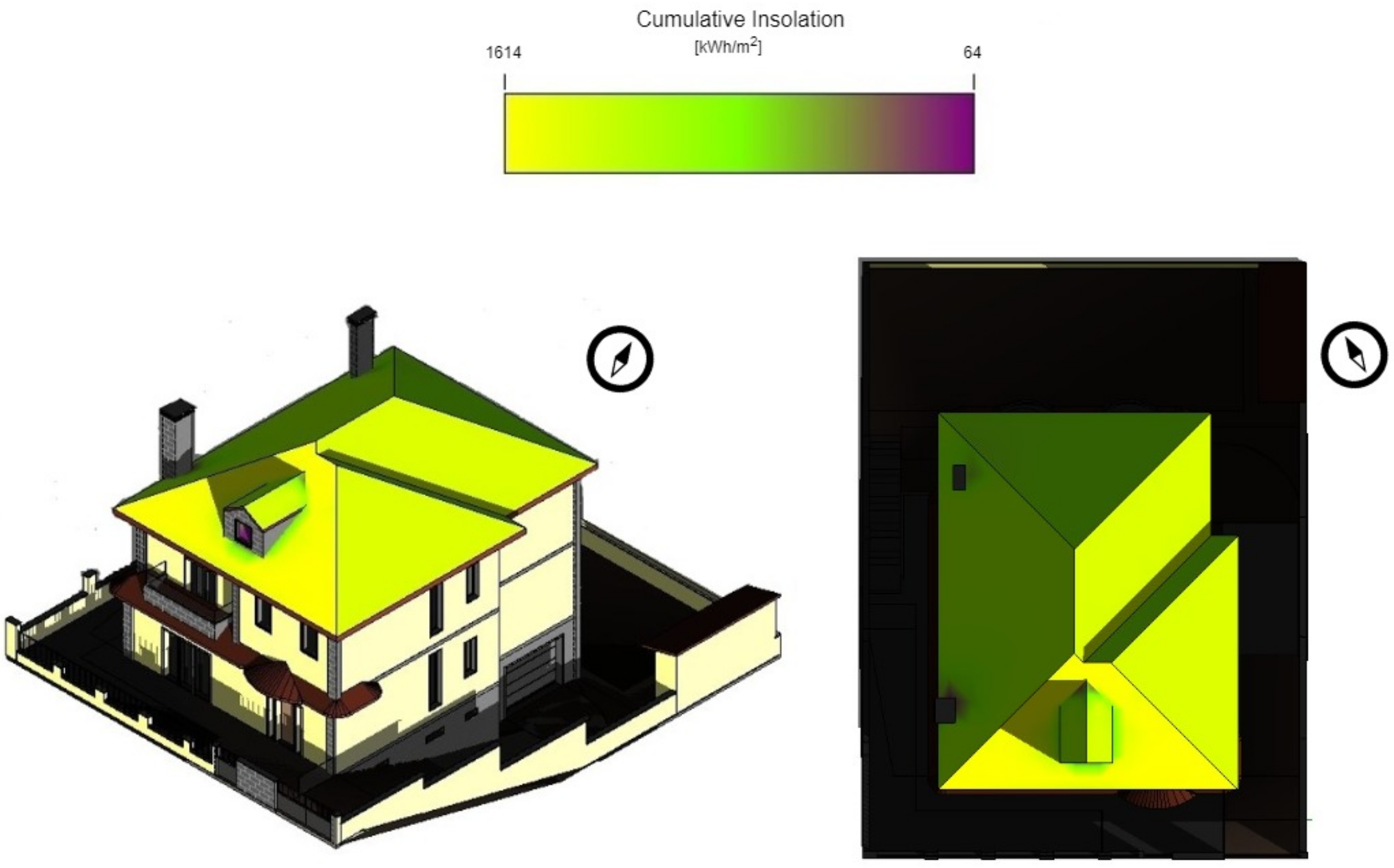
The infrastructure under analysis is a residential property in Santa Iria de Azoia. Castro Verde and Vila Real are other locations to be studied in order to evaluate the photovoltaic system performance. The simulation results are shown in Figure 1. It is possible to verify with the colour coding that the part of the roof facing south is the one that has the most sun exposure. However, the shadow caused by the window on the top floor of the property and the fact that the area available for the placement of solar panels is smaller makes the east-facing part of the roof the choice, which is the second part of the roof with greater solar exposure [7].

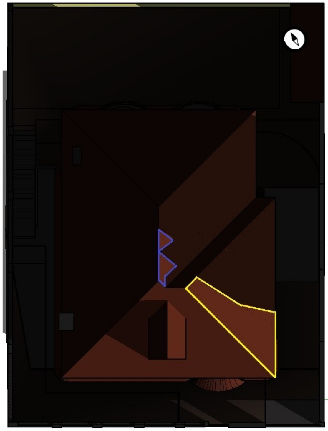
Figure 2 presents the result of the simulation of the shading effect on the infrastructure roof during one year of analysis. The area outlined in yellow corresponds to the useful area of the roof that is not affected by annual shading, and the zone delimited in blue, due to its reduced area, will not affect the generator. Due to the limitations of the Autodesk Revit 2022^® programme, the area outlined in yellow is 12 m${}^2$, which corresponds to an approximated value.

5.3. Photovoltaic System Sizing

The optimisation algorithm presents as the best solution the generators whose data are inserted in

Table 1. Photovoltaic system sizing for the three places.

	M	N
c-Si	9	4
CIGS	10	6
c-Si NWs	9	9
CsPbI${}_{\mathbf{3}}$ QDs	7	6

[7]. Regarding the number of viable properties to be fed by the generator, the algorithm presents as an optimal solution that only one is possible [7].

For these generators, the characteristics of the inverters chosen and the cables and protection devices correspond to the values shown in

Table 2. Inverters and DC sizing.

		Inverters				DC Sizing
						Row Cable			Fuses	Main DC Cable
		P${}_{\mathit{n}}^{\mathrm{inv}}$ [kW]	V${}_{\mathit{min}}^{\mathrm{inv}}$ [V]	V${}_{\mathit{max}}^{\mathrm{inv}}$ [V]	I${}_{\mathit{max}}^{\mathrm{inv}}$ [A]	I${}_{\mathit{z}}$ [A]	s [mm${}^{\mathbf{2}}$]	L${}_{\mathit{max}}$ [m]	I${}_{\mathit{z}}$ [A]	I${}_{\mathit{z}}$ [A]	s [mm${}^{\mathbf{2}}$]	L${}_{\mathit{max}}$ [m]
Santa Iria de Azoia	c-Si	[9.622; 16.495]	$]-\infty$; 167]	[373; $+\infty [$	[41; $+\infty [$	14.303	2.5	25.572	16	25.480	6	22.963
	CIGS	[9.883; 16.942]	$]-\infty$; 180]	[370; $+\infty [$	[42; $+\infty [$	9.737	2.5	37.249	10	26.021	6	22.807
	c-Si NWs	[7.456; 12.782]	$]-\infty$; 102]	[284; $+\infty [$	[43; $+\infty [$	6.65	2.5	41.819	6	26.662	10	26.297
	CsPbI${}_{\mathbf{3}}$ QDs	[5.631; 9.653]	$]-\infty$; 91]	[276; $+\infty [$	[34; $+\infty [$	7.94	2.5	34.058	8	21.222	10	32.022
Castro Verde	c-Si	[9.855; 16.894]	$]-\infty$; 160]	[376; $+\infty [$	[41; $+\infty [$	14.492	2.5	25.767	16	25.480	6	22.963
	CIGS	[10.111; 17.334]	$]-\infty$; 174]	[372; $+\infty [$	[42; $+\infty [$	9.866	2.5	37.501	10	26.021	6	22.807
	c-Si NWs	[7.670; 13.148]	$]-\infty$; 96]	[287; $+\infty [$	[43; $+\infty [$	6.740	2.5	42.272	6	26.662	10	26.297
	CsPbI${}_{\mathbf{3}}$ QDs	[5.775; 9.899]	$]-\infty$; 86]	[278; $+\infty [$	[34; $+\infty [$	8.047	2.5	34.328	8	21.222	10	32.022
Vila Real	c-Si	[9.991; 17.127]	$]-\infty$; 169]	[379; $+\infty [$	[41; $+\infty [$	14.504	2.5	26.001	16	25.480	6	22.963
	CIGS	[10.237; 17.550]	$]-\infty$; 181]	[375; $+\infty [$	[42; $+\infty [$	9.875	2.5	37.802	10	26.021	6	22.807
	c-Si NWs	[7.816; 13.3993]	$]-\infty$; 103]	[290; $+\infty [$	[43; $+\infty [$	6.745	2.5	42.823	6	26.662	10	26.297
	CsPbI${}_{\mathbf{3}}$ QDs	[5.861; 10.048]	$]-\infty$; 92]	[281; $+\infty [$	[34; $+\infty [$	8.054	2.5	34.643	8	21.222	10	32.022

[7].

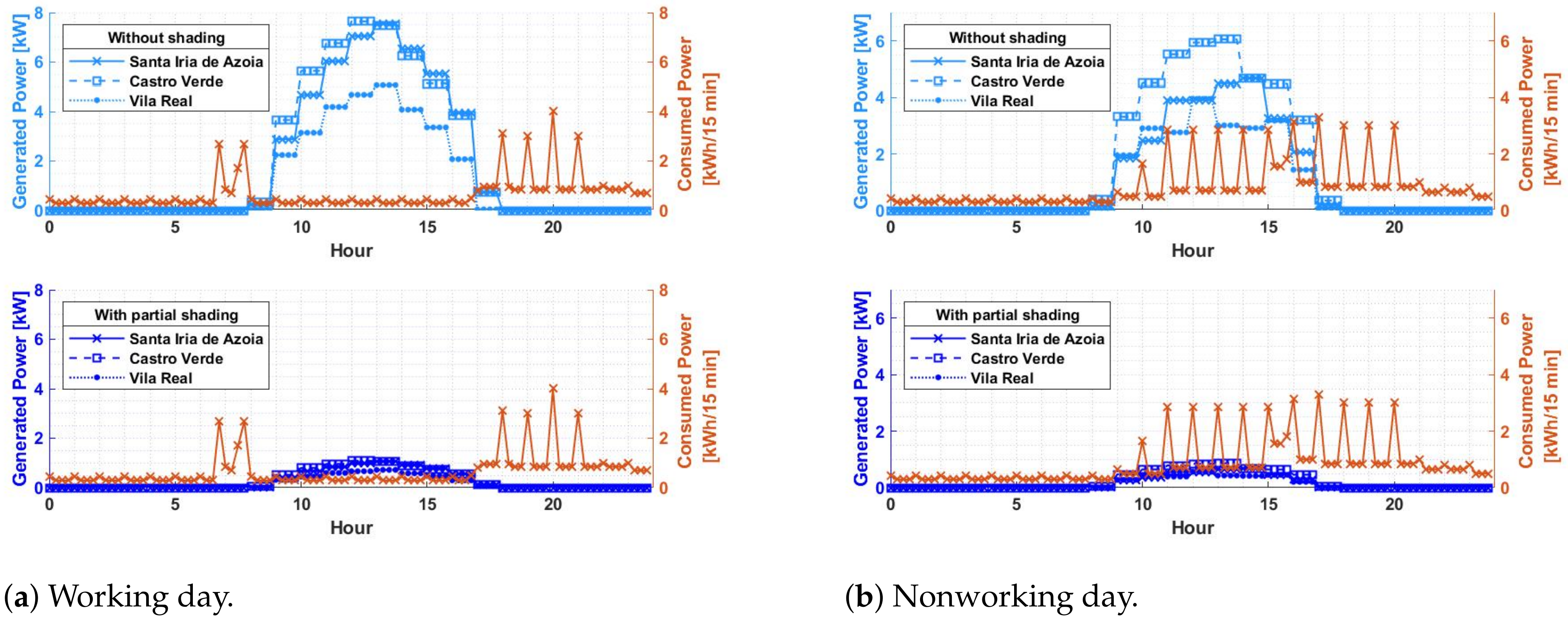
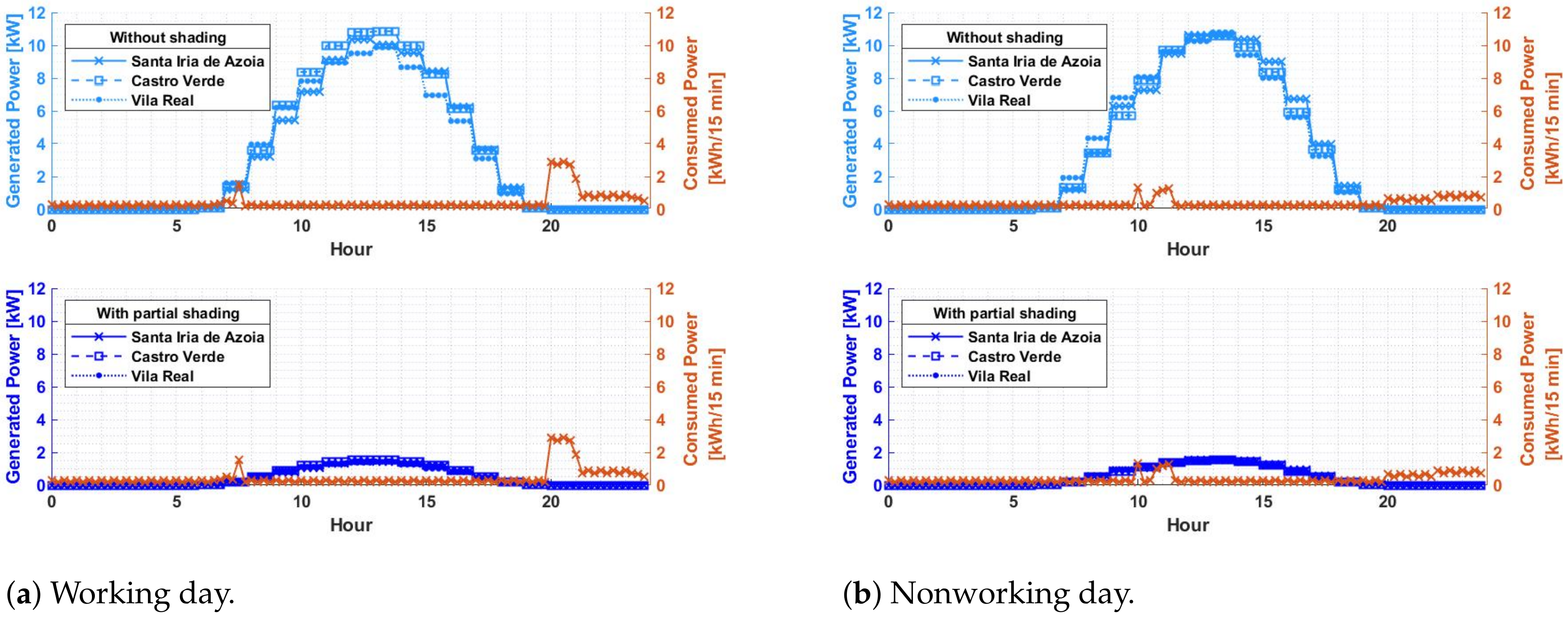
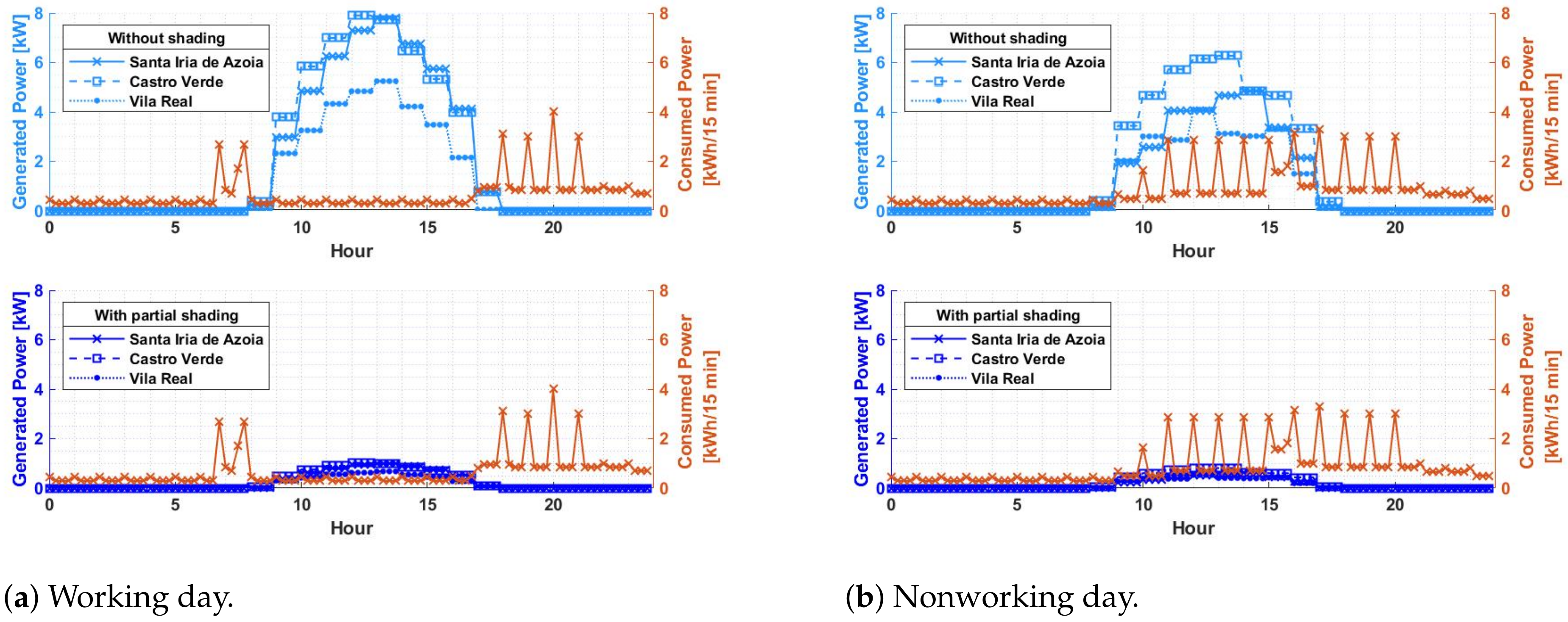
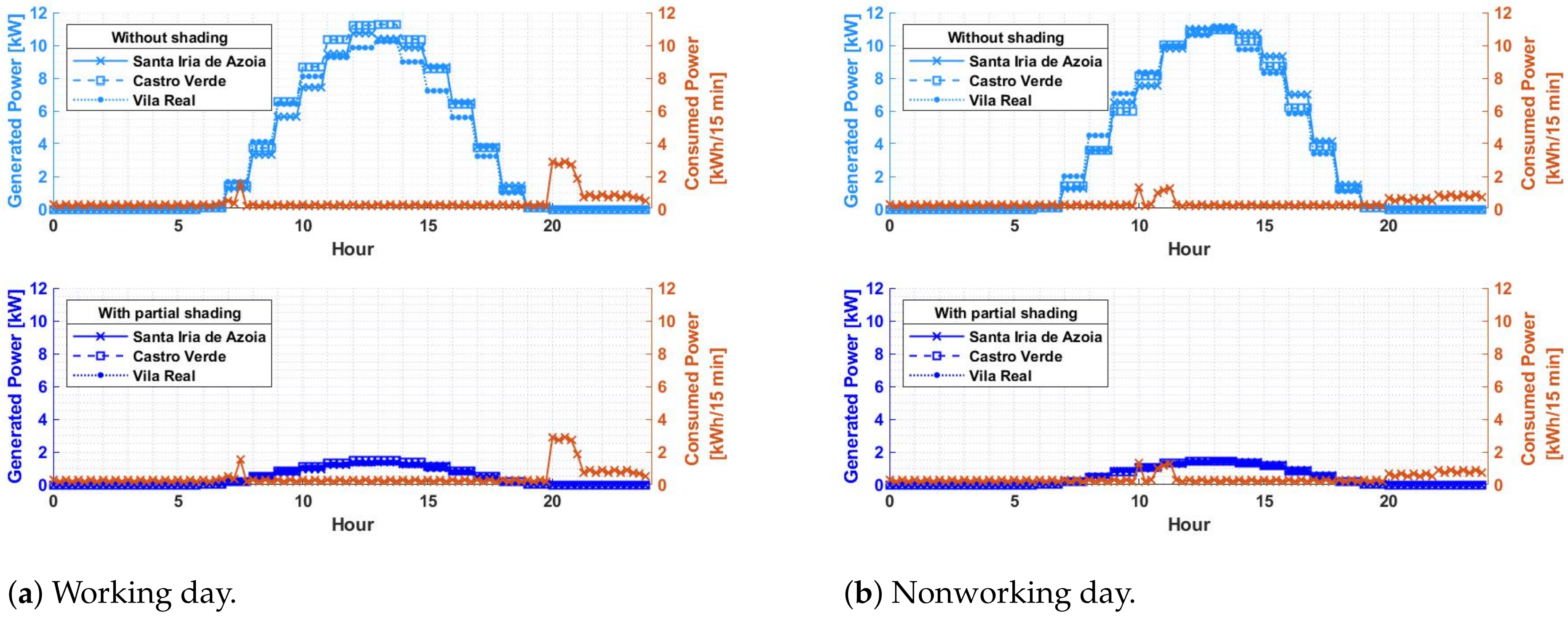
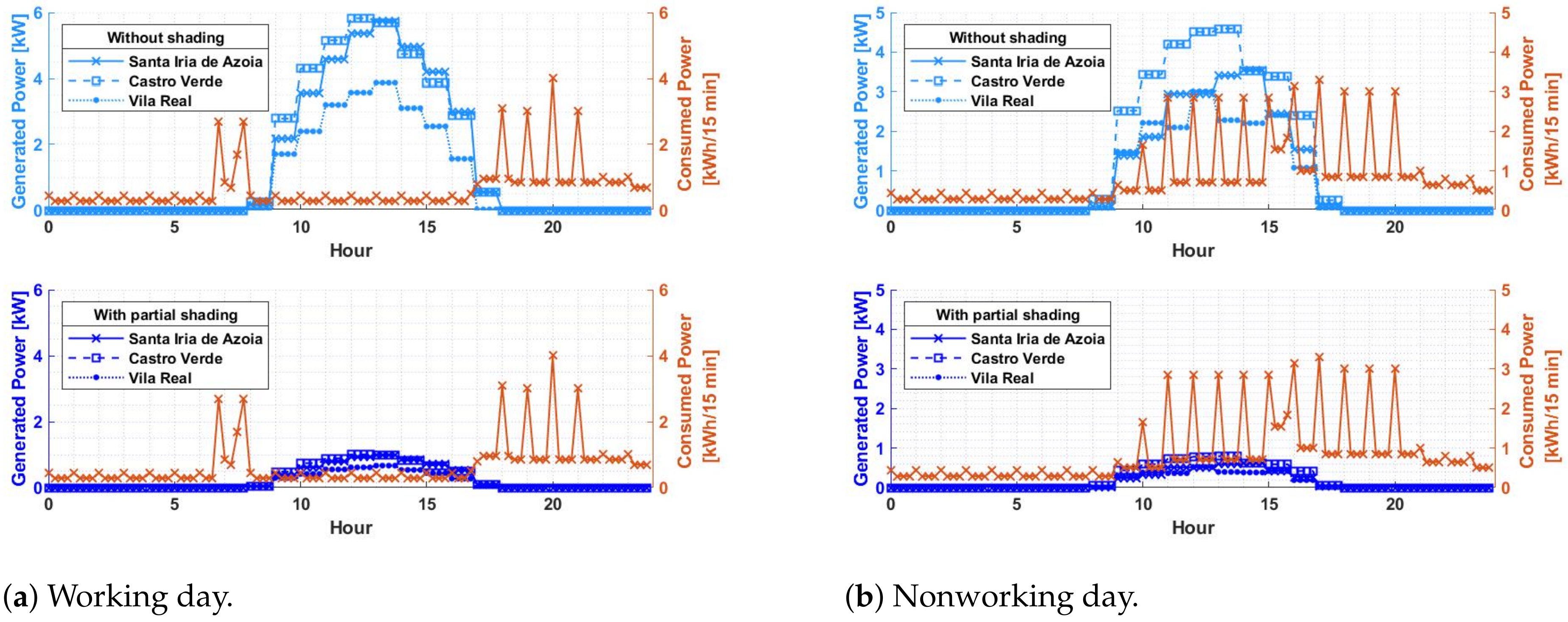
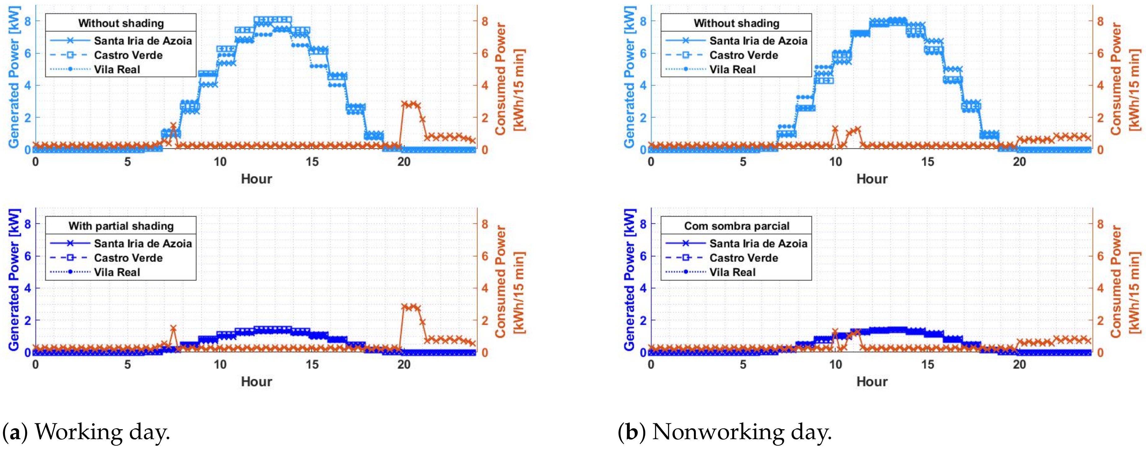
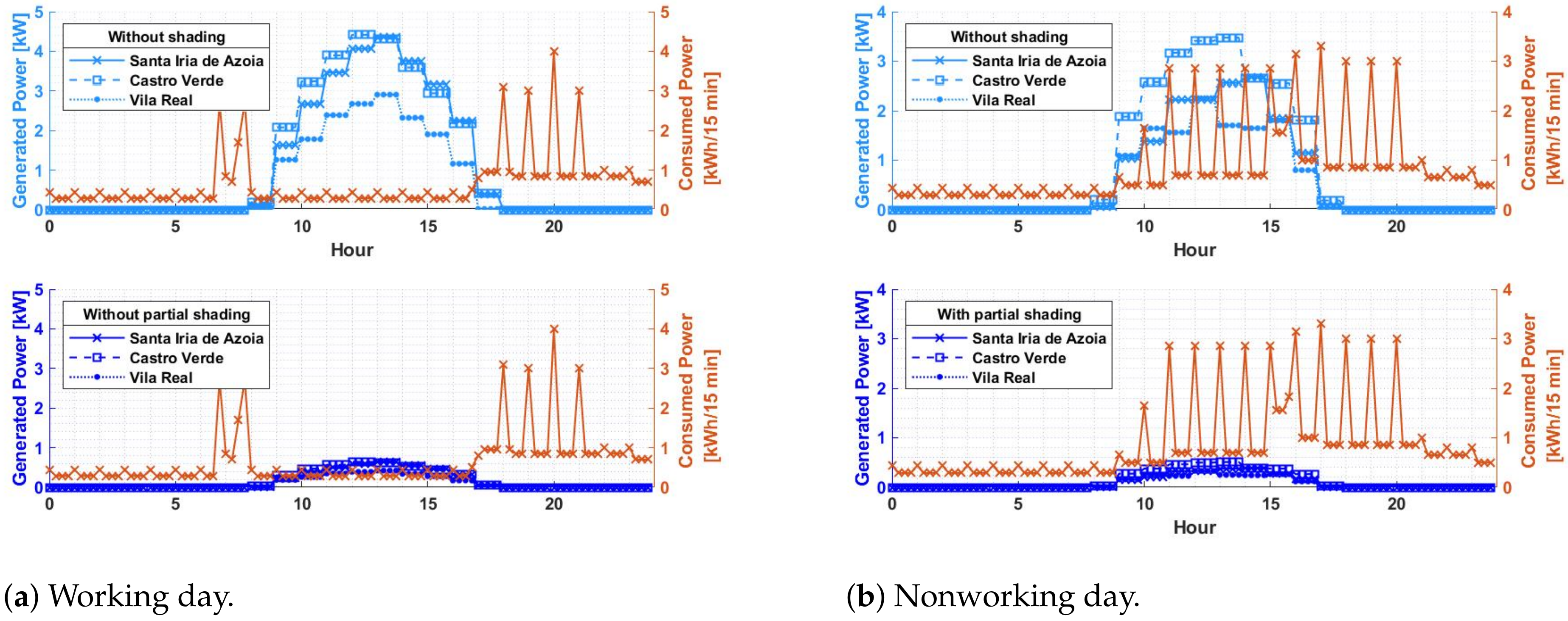
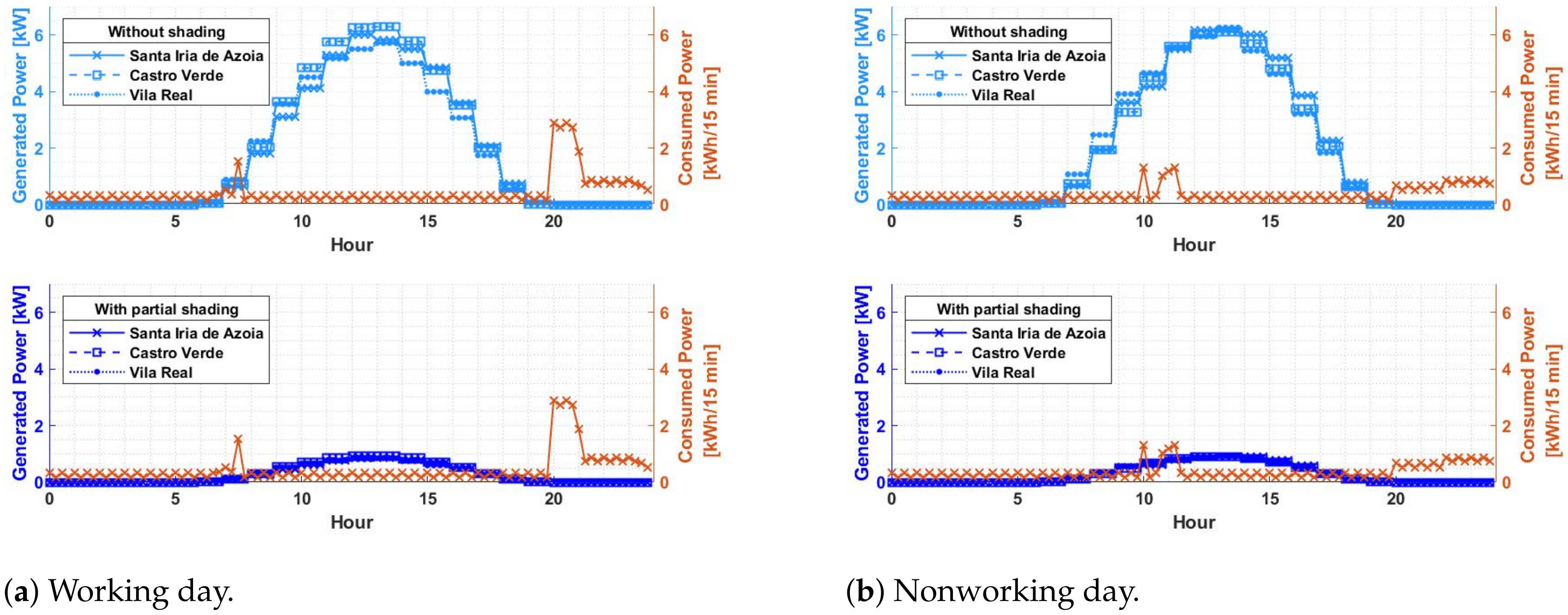
For the optimised generators (Table 1), when the shading effect occurs the production level decreases from 13% to 17.5% at STC conditions, depending on the technologies used. Following the methodology presented in Section 4.3, the consumption–generation curves for two significant days of the extreme consumption months (January and August), with and without the application of partial shading, are presented in Figure 3, Figure 4, Figure 5, Figure 6, Figure 7, Figure 8, Figure 9 and Figure 10. The aim is to present the curves in a qualitative and visual way, abstracting from the quantitative values. In this way, it is possible to analyse for each time interval whether the load is covered by the generator under study.

Note that there is a discrepancy in production according to the place under study due to varying atmospheric conditions. These affect the performance of solar technologies. Note also that the maximum generated power using modules from emerging technologies is lower than the maximum production when traditional technologies are used. Finally, the generation curves with partial shading present lower values when compared with the generation curves without the shading effect, and in some instances, the generation curve is not able to cope with the load.

5.4. Financial Indicators for Project Evaluation

In order to obtain the financial indicators for project evaluation, the annual cash flows have to be obtained. Through the literature information, we found the initial investment values for all technologies under analysis, which are presented in

Table 3. Initial investment for different photovoltaic generators, using different technologies.

	c-Si	CIGS	c-Si NWs	CsPbI${}_3$ QDs
${\mathit{I}}_{\mathbf{0}}$[€]	8088.118	12,398.863	14,056.454	10,800.134

. For solar nanotechnologies, the value used for the module degradation factor corresponds to the highest one presented in Section 2 (0.96%/year).

In order to verify when the photovoltaic system would no longer support the load in its entirety, a financial analysis was conducted an extended period of time, which was 1000 years. When the photovoltaic system is no longer able to support the load, that is, the load consumption is higher than the generator production in all time intervals, the system has zero viability, and the year in which this happens is called the year of zero viability.

The optimised financial results for the scenario with and without the partial shading effect are presented in

Table 4. Financial indicators in the three locations under analysis, where the values highlighted in green correspond to those with a $PR$ of less than 10 years.

		Without Selling to the Grid		With Selling to the Grid		Viability in 1st Year [%]	Year of Zero Viability
		$\mathit{NPV}$ [€]	$\mathit{PP}$ [Years]	$\mathit{NPV}$ [€]	$\mathit{PP}$ [Years]
Santa Iria de Azoia	c-Si	−25,902.288	∞	19,588.346	$\boxed{\mathrm{4.434}}$	44.178	647
	CIGS	−33,167.066	∞	11,811.527	$\boxed{\mathrm{6.858}}$	44.238	435
	c-Si NWs	−35,521.716	∞	−5353.050	20.743	43.188	402
	CsPbI${}_{\mathbf{3}}$ QDs	−30,079.375	∞	−9001.194	∞	42.158	375
Castro Verde	c-Si	−25,926.163	∞	23,145.022	$\boxed{\mathrm{3.968}}$	44.481	650
	CIGS	−33,149.910	∞	15,364.535	$\boxed{\mathrm{6.059}}$	45.088	437
	c-Si NWs	−35,414.614	∞	−2891.284	15.927	43.467	403
	CsPbI${}_{\mathbf{3}}$ QDs	−29,963.774	∞	−7033.547	∞	42.529	377
Vila Real	c-Si	−26,136.880	∞	15,899.477	$\boxed{\mathrm{3.968}}$	43.898	650
	CIGS	−33,408.105	∞	8124.153	$\boxed{\mathrm{7.955}}$	43.993	436
	c-Si NWs	−35,830.063	∞	−7890.932	∞	42.760	403
	CsPbI${}_{\mathbf{3}}$ QDs	−30,510.232	∞	−11,029.577	∞	41.104	376

and

Table 5. Financial indicators in the three locations under analysis, with partial shading applied.

		Without Selling to the Grid		With Selling to the Grid		Viability in 1st Year [%]	Year of Zero Viability
		$\mathit{NPV}$ [€]	$\mathit{PP}$ [Years]	$\mathit{NPV}$ [€]	$\mathit{PP}$ [Years]
Santa Iria de Azoia	c-Si	−30,077.604	∞	−28,487.070	∞	33.370	345
	CIGS	−37,620.142	∞	−36,555.198	∞	32.991	223
	c-Si NWs	−39,560.585	∞	−38,606.909	∞	32.160	221
	CsPbI${}_{\mathbf{3}}$ QDs	−34,857.081	∞	−35,184.148	∞	26.741	176
Castro Verde	c-Si	−29,850.777	∞	−27,963.636	∞	34.700	349
	CIGS	−37,394.882	∞	−36,082.597	∞	33.816	226
	c-Si NWs	−39,334.671	∞	−38,161.563	∞	33.319	223
	CsPbI${}_{\mathbf{3}}$ QDs	−34,649.456	∞	−34,885.575	∞	27.911	179
Vila Real	c-Si	−30,391.133	∞	−29,031.360	∞	32.186	347
	CIGS	−37,931.620	∞	−37,047.202	∞	31.655	225
	c-Si NWs	−39,858.946	∞	−39,068.720	∞	31.504	222
	CsPbI${}_{\mathbf{3}}$ QDs	−35,199.583	∞	−35,493.454	∞	25.117	178

.

In these Tables, if there is no sale of the surplus to the grid, the $PP$ is presented as being infinite (∞). This means that in the period under analysis, there was no recovery of the initial investment. It is important to point out that if the $PP$ does not occur until the zero viability year, the project will never have the investment paid and thus the project becomes economically completely impossible. It is important to note that this analysis period can be changed, and the same algorithm can be put into practice since it is prepared for eventual changes by the user.

A deeper analysis of both tables will be conducted in the next section.

6. Discussion

The results’ discussion takes into account the physical, economic, social and environmental factors. The entire discussion is based on the analysis performed using the optimisation algorithm, and results can be found in Table 4 and Table 5.

6.1. Physical Factors

The location of the generator is one of the factors that affects the performance of the photovoltaic system. Santa Iria de Azoia, Castro Verde, and Vila Real were chosen for the analysis because they are located in different areas of Portugal that present discrepancies in temperature and irradiance.

Castro Verde presents the highest values of energy produced during all days in January and on the working days of August due to higher average temperature and irradiance values, except for August nonworking days. Regarding August nonworking days, the highest generation values are reached in Vila Real. This is justified by the simple fact that the local average temperature throughout the nonworking days is lower than the average temperatures experienced in the other places. The huge impact of the temperature variation on higher values of energy production is therefore confirmed.

From the economic point of view and by analysis of Table 4, Castro Verde is the place that best satisfies the investor due to the high production of the generators, and in terms of the $PP$, using traditional technologies, the costs are recovered more quickly. Concerning the viability of the sized systems, in the first year of analysis, Castro Verde presents the highest values, so there are more times when production is higher than consumption. With the CIGS technology, the highest viability is obtained without shading in the generator, and the value is 45.088%. This means that in 45.088% of the considered time intervals throughout the year, production exceeds consumption. It can also be seen that the use of c-Si NWs and CsPbI${}_3$ QDs modules translates into lower viability than that achieved with c-Si and CIGS technologies.

6.2. Financial Indicators for Project Evaluation

According to Table 4, it is possible to analyse the financial indicators from two points of view: no sale of the surplus production to the grid and its sale. The fact that there is a production surplus and the investor does not benefit from it by delivering the surplus to the grid at zero cost, implies that the project is not economically viable, which results in a negative $NPV$, regardless of the solar technology and place analysed. This leads to a decrease in investment in renewable energy systems and the continued use of non-renewable energy. In addition, the $PP$ shows that the investment cannot be recovered over the period under analysis. The installation of systems using renewable energy sources ends up being beneficial to the investor if his monthly electricity bill is lower, and this reduction should be subtracted from the value of the initial investment. Nevertheless, in the medium-long term it will not be possible to recover the monetary investment.

The sale of the surplus production to the grid leads, in some cases, to nonviable projects, demonstrated through the financial indicators presented in Table 4. Note that the use of traditional technologies, in any of the places considered, leads to a positive $NPV$, which translates to the economic viability of the project, covering the initial investment and obtaining the minimum remuneration required by the investor. Furthermore, the $PP$ is lower than 10 years, being that it ends up covering the warranties of the equipment used and in addition the lifetime of the photovoltaic panels [19]. On the other hand, the use of emerging technologies is not viable, presenting a negative $NPV$. However, the c-Si NWs technology presents a $PP$ of 15–20 years, which is exceeds some of the warranties of the equipment used, and in case of failure, the investor will be responsible for new investment, making the project more expensive and further increasing its $PP$. Because energy production using nanocells is not so high, there is less surplus when compared with traditional technologies. Consequently, this lower production of c-Si NWs and CsPbI${}_3$ QDs makes it neither economically beneficial nor viable for the investor. In this situation, the investor ends up benefiting from a reduction in electricity bills and simultaneously collecting the equivalent of its surplus production. Therefore, on a financial level, it is beneficial in two respects and ends up being an incentive for investment in renewable energy systems for self-consumption.

6.3. Social Factors

The fact that there are no batteries and the system is on-grid leads to a loss of the surplus produced energy. Obviously, there can be a financial return with the non-consumed surplus energy. However, from the point of view of production and not storage, it ends up being lost energy. The reason at they are prohibitively expensive [33]. By analysing Figure 3, Figure 4, Figure 5, Figure 6, Figure 7, Figure 8, Figure 9 and Figure 10, it can be seen that there is a large discrepancy, particularly during the working days, between the consumption and the production peaks in each time interval. Therefore, in order to take advantage of the surplus energy production and not lose it, the concept of a smart city can be applied. Commercial establishments in the locale of the photovoltaic installation could benefit from energy from the installation. If we consider that the commercial establishments’ consumption is higher during sunny hours, when e consumption in the infrastructure under analysis is lower, the commercial establishments could use the surplus production. This would be a way of contributing to the decrease in the use of energy from non-renewable sources. This way, it is possible to create more energy-efficient cities and contribute to fighting climate change. This solution ultimately ensures a reduction of energy consumption from the grid in several properties, which implies the reduction of greenhouse gas emissions associated with its production, ultimately contributing to the adaptation of cities to climate change.

6.4. Environmental Factors

The use of renewable energies greatly promotes the decrease in the emission of greenhouse gases, since the production of green energies occurs sustainably without causing pollution. The energy that a citizen consumes from the grid is energy resulting from resources, which sooner or later will be exhausted. Table 4 shows that, according to the technology used, the number of years until zero viability changes according to the place under analysis, taking on average around 649, 436, 303, and 376 years. although the systems under analysis will certainly not last even 200 years, during their life cycle, they will be generating electricity with renewable resources, meaning that during these years, less energy is produced from non-renewable energy sources thereby helping limit climate change.

6.5. Shading Effect

Total or partial shading on photovoltaic systems will always occur. It is simply unavoidable. Figure 3, Figure 4, Figure 5, Figure 6, Figure 7, Figure 8, Figure 9 and Figure 10, verify through the production curves that during partial shading the system cannot meet demand in most of the time intervals in all locations under analysis and with photovoltaic technologies used. This implies that the investor will have to use energy from the grid. The production of surplus energy occurs mainly on working days, due to the reduced demand and increased production during sunny hours. However, the amount of surplus energy does not make up for that lost through shading scenarios.

By analysis of Table 5, regardless of whether there is a sale of surplus energy to the grid, the $NPV$ is negative for all technologies and locations, which indicates the clear nonviability of the project. Furthermore, for the period under analysis, there is no $PP$, which indicates that the investor will never recover the investment. Nevertheless, even if the surplus energy produced is delivered to the grid at zero cost, the use of the photovoltaic generator ends up being beneficial to the investor if the focus is the reduction of monthly electricity bills and not the investment he will have to make. However, with the existence of partial shading, these reductions translate into lower values if compared with a no shading scenario. Considering the existence of partial shading, from year 0 to year 1 of the analysis, the reduction in utility bills is around 43% to 48% when using c-Si or CIGS modules, and around 35% to 46% when using technologies with nanostructures.

Lastly, it can be seen that partial shading causes a decrease of between 10 and 16% of energy production compared to the shade-free scenario. The number of years until zero viability decreases to about half in the shading scenarios. This is justified by the fact that the production points in the partially shaded scenarios are not much higher than the consumption points in each time interval when compared to the non-shading scenarios, so, although module degradation occurs at the same rate, it takes less time before all production points are lower than the consumption ones.

7. Closing Remarks

In this paper, different solar technologies integrated into a self-consumption power supply system for three locations in Portugal are analysed with and without a partial shading effect. For each traditional and emerging technology, both the photovoltaic system sizing and the financial viability are presented.

Using a self-consumption system allows the investor to have lower monthly bills, and at the same time reduce carbon emissions. Enabling self-consumption unleashes private investment into the energy transition, and it is a potentially cost-effective strategy for countries to meet energy and climate targets. These self-consumption systems do not need huge areas for their implementation, they have a reduced environmental impact and could be a system that guarantees energy self-sufficiency. Besides that, these constitute lower costs for each government associated with non-renewable energies, and the operation and maintenance costs of grid systems are lower [34,35].

The analysis carried out with partial shading and non-shading on the different generators shows that shade is a problem for good performance of photovoltaic generators, decreasing production between 13% to 17.5%. At the level of production in each time interval considered, the consumption–generation curves show that the shadow allows most of the load consumption peaks to be unsupported, which from an economic point of view translates into clear nonviability for the project, with or without the sale of the surplus production, regardless of the technology used or region under analysis. On the other hand, the lack of shading allows the generator to cover most of the load consumption peaks during sunny hours. In the case of selling surplus energy to the grid, the use of traditional technologies allows the project to be economically viable, presenting a $PP$ lower than 10 years, and covering the warranties of the different equipment. Emerging technologies have shown not to be, for now, the best solution for photovoltaic generators since the production of these generators is lower than the production of generators using traditional technologies. In addition, emerging technologies present lower viability in the first year of analysis than generators using traditional technologies. If the surplus energy production is delivered at zero cost to the grid, then the project becomes nonviable, regardless of the solar technology used and place under analysis.

Due to the absence of batteries, the surplus energy produced is not stored to be used when no production occurs. From a social point of view and in order to reduce the consumption of energy from the public grid, this surplus energy would be well used to supply commercial establishments nearby the infrastructure under analysis, contributing to the reduction of greenhouse gas emissions associated with the production of energy from the grid, and consequently, fighting climate change, which is a big problem around the world [36].

Although from 2005 until 2019, Portugal reduced its per capita greenhouse gas emissions by 20%, the country has to reduce these levels of global greenhouse gas emissions until 2050, due to the Paris agreement [36]. To achieve that, a tax on CO${}_2$ was created. From 2012 until 2017, the value was about €4–7 per ton of CO${}_2$, and since 2018, it increased to €24 per ton of CO${}_2$. In 2021, the explicit tax on CO${}_2$ reached a record value of €47.91 per ton of CO${}_2$ [37]. This shows the importance that energy transition has and the role that governments have in this topic.

The role of governments in implementing measures that promote investment in renewable energy is crucial, being important in determining a fixed value for the sale of surplus energy to the grid. Otherwise, the possibility of practising almost zero values for the sale of surplus energy to the grid prevents investors from taking part in the projects.

In addition, the location of photovoltaic arrays needs to be carefully considered to avoid barriers to solar production such as shading that may prevent the system from operating at its full potential.