Path-Following Control for Thrust-Vectored Hypersonic Aircraft

Abstract

Thrust vector control (TVC) might be used to control aircraft at large altitudes and in post-stall conditions when aerodynamic control surfaces are ineffective. This study demonstrated that the implementation of the TVC on high-speed aircraft is a reasonable solution and might be an alternative when compared to the complicated reaction control system or large aerodynamic control surfaces. The numerical flight dynamics model of the X-15 experimental aircraft was developed and implemented in MATLAB/Simulink and then used to investigate the proposed solution. The obtained results indicate that the aircraft, equipped with full 3D thrust vectoring and two independent horizontal stabilizers to control the roll angle, was able to achieve flight along the path that was defined by a set of waypoints. This paper also highlights the potential benefits and challenges of using TVC as a control method for aircraft. The results of this study contribute to the growing body of research on aircraft control and simulation. Future work can explore the use of TVC for other aircraft with unique configurations and low maneuverability features.

1. Introduction

The effectiveness of movable aerodynamic control surfaces depends on the flight speed and the density of the air. Control surfaces lose their effectiveness quickly at low flight speeds [1]. Moreover, at high altitudes, as the density of the air decreases, these aerodynamic control surfaces cannot guarantee a proper object response. On the other hand, at supersonic speeds, aerodynamic heating could complicate the task even more. To overcome the problems mentioned above, thrust vectoring control (TVC) might be used. TVC might be divided into two main categories: mechanical and fluidic [2,3,4,5,6,7,8]. To realize the mechanical actuation of TVC, several technological methods could be used: gimbaled engines, Vernier thrusters, jet vanes, axial plates, movable nozzles, etc. There exists various kinds of fluidic thrust vectoring [9]: shock wave TVC, bypass shock wave TVC, coflowing TVC, counterflowing TVC, dual throat nozzle TVC and bypass dual throat nozzle TVC.

In this article, the research concentrated on the main motor thrust deflection for hypersonic vehicles using mechanical devices. Furthermore, several designs such as tiltrotors (for example, V-22 Osprey) or vertical and/or short take-off and landing aircraft (e.g., Harrier), are often classified in the TVC category, but these are outside the scope of the presented study.

The existing literature often refers to the application of TVC on military fighter aircraft. Liu et al. [10] developed three independent controllers for three channels to realize the Herbst maneuver. Zhou et al. [11] investigated the usage of the L1 Adaptive Control Law on a small-scale model of F35B. Dinca and Corcau [12] investigated the use of TVC combined with canard control surfaces but in the context of a low-speed vehicle. Raghavendra et al. [13] addressed the problem of spin recovery without and with the use of TVC. Yushan et al. [14] contributed to the topic of using TVC in the take-off phase of flight but did not present the detailed results. The results of the experimental measurements of fluidic TVC were reported by Neely et al. [15], but were without an extensive flight dynamics simulation analysis. Practically, thrust vectoring was used by several military jets to significantly increase maneuverability [16]. With the use of TVC, effective control at large angles of attack in the post-stall region might be achieved [17]. For delta-shaped wings, the maximum range of the angles of attack is up to 35${}^{\circ }$, as suggested in [18]. TVC is used in Russian fighters such as the Su-27 [19], Su-35 [20,21] and MIG 29 OVT. The nozzles operate in one plane but are canted 32${}^{\circ }$ outward from the engine axis. In that way, it is possible to realize the change in aircraft orientation in the pitch and yaw planes. TVC is also considered as an upgrade for the EJ200 engine that is used on a Typhoon Eurofighter [22,23]. The F-22 [24] adopted thrust vectoring in one plane. Both nozzles are parallel and could influence only the pitch rate of the aircraft. Yaw rate control was not used because it requires a more sophisticated mechanism to lower the stealth capabilities. There were a number of experimental technology demonstrators (X-31, F-15-STOL/MTD, X-62 VISTA, and F-18 HARV), but they did not come into mass production [20,25,26].

However, even for aircraft, this type of control is not widely used due to several disadvantages. It requires additional mass and volume. In addition, it increases the complexity of the system, and the risk of failure is higher when compared to typical engines. This mechanism increases maintenance costs. Using only control surfaces at high altitudes is very ineffective.

Several studies presented the implementation of flight simulation models for various other research topics in aerial vehicle control. The kind of actuator assumed in the study is used in space rockets due to the fact that it can operate in the vacuum of space, where classical aerodynamic control surfaces cease to be effective. Jenie et al. [27] investigated the control of the Falcon 9 rocket using thrust vectoring. The topic of TVC and similar solutions gained significant attention among missile engineers over the years, in the context of military applications. Moreover, recently, several interesting studies were presented. For example, Liu and Wang [28] investigated the use of TVC to realize the rapid turn in the vertical launch missile system. Studies such as [29] focused on the use of lateral thrusters to reduce the impact point dispersion. Meanwhile, Glebocki and Jacewicz [30] investigated the use of gasodynamic control together with a modified guidance scheme for rocket artillery projectiles. Finally, Glebocki and Jacewicz [31,32] analyzed the use of small lateral thrusters to realize the cold vertical launch of the projectile. From a practical point of view, several military projectiles, such as AIM-X9 [33,34] and MICA [35], use TVC to increase agility.

The use of TVC for hypersonic vehicles was also investigated, but it seems that it was investigated with less attention when compared to the previously mentioned topics. The appropriate design of the control system is one of the most demanding tasks in the development of a hypersonic vehicle. An excellent survey of control methods that can be adopted for high-speed vehicles was presented by Bin and ZhongKe [36]. Ding et al. [37] discussed the comparison of various control methods of hypersonic vehicles. However, they also presented a review of the guidance laws. Bliamis et al. [38] proposed the shock control bump concept but presented only the results of the CFD analysis. Falkiewicz et al. [39] presented an analysis of how to include the aerothermoelastic effects into the simulation of a hypersonic vehicle. Moreover, Chen et al. [40] studied the use of the L1 adaptive control for a model of the generic hypersonic vehicle.

It was obtained that in the literature there exists a significant gap on the topic of TVC in the context of hypersonic vehicles with very limited control authority. The existing studies often concentrate on the application of TVC on military fighters or on missiles to increase its maneuverability.

The primary motivation for the presented study was to investigate the feasibility of the main motor TVC for a high-speed vehicle. The X-15 vehicle’s aircraft was chosen as a test platform due to its non-standard configuration and low maneuverability features. One of the most important challenges is the high-damping of the lateral motion that is caused by the large vertical stabilizers. Moreover, this vehicle is quite well documented in publicly available reports, and the geometric, mass and aerodynamic data are obtainable.

The main contribution of this paper is the implementation of the path-following control that is achieved by using the TVC control algorithm for the X-15 experimental aircraft. The aircraft was assumed to be equipped with a full 3D thrust vectoring system and two independent movable horizontal stabilizers that when deflected differentially are used to control the roll angle. That means the thrust might be deflected in pitch and yaw planes. This configuration is rather typical for military projectiles and is rarely used in aircraft. Using TVC might be a reasonable alternative to a reaction control system or large movable aerodynamic control surfaces. Furthermore, the X-15 was not designed to perform maneuvers at high speeds, as the object was designed to fly along a straight path. The unusual configuration with the low aspect ratio makes maneuvering difficult without putting additional strain on the aircraft structure or the pilot in command. Realizing agile maneuvers at a high speed leads to high g-loads. The abovementioned problem occurs regardless of which actuation method is used (TVC, reaction control system, or aerodynamic control surfaces).

The organization of the remainder of this article is as follows: In Section 2, the modified X-15 test platform was briefly described. This is followed by Section 3, in which the flight simulation model of the object was presented. In Section 4, the control system structure was shown. In Section 5, the obtained results are presented and discussed. The article ends with a summary of the main findings. Moreover, further research directions are suggested.

2. Test Vehicle

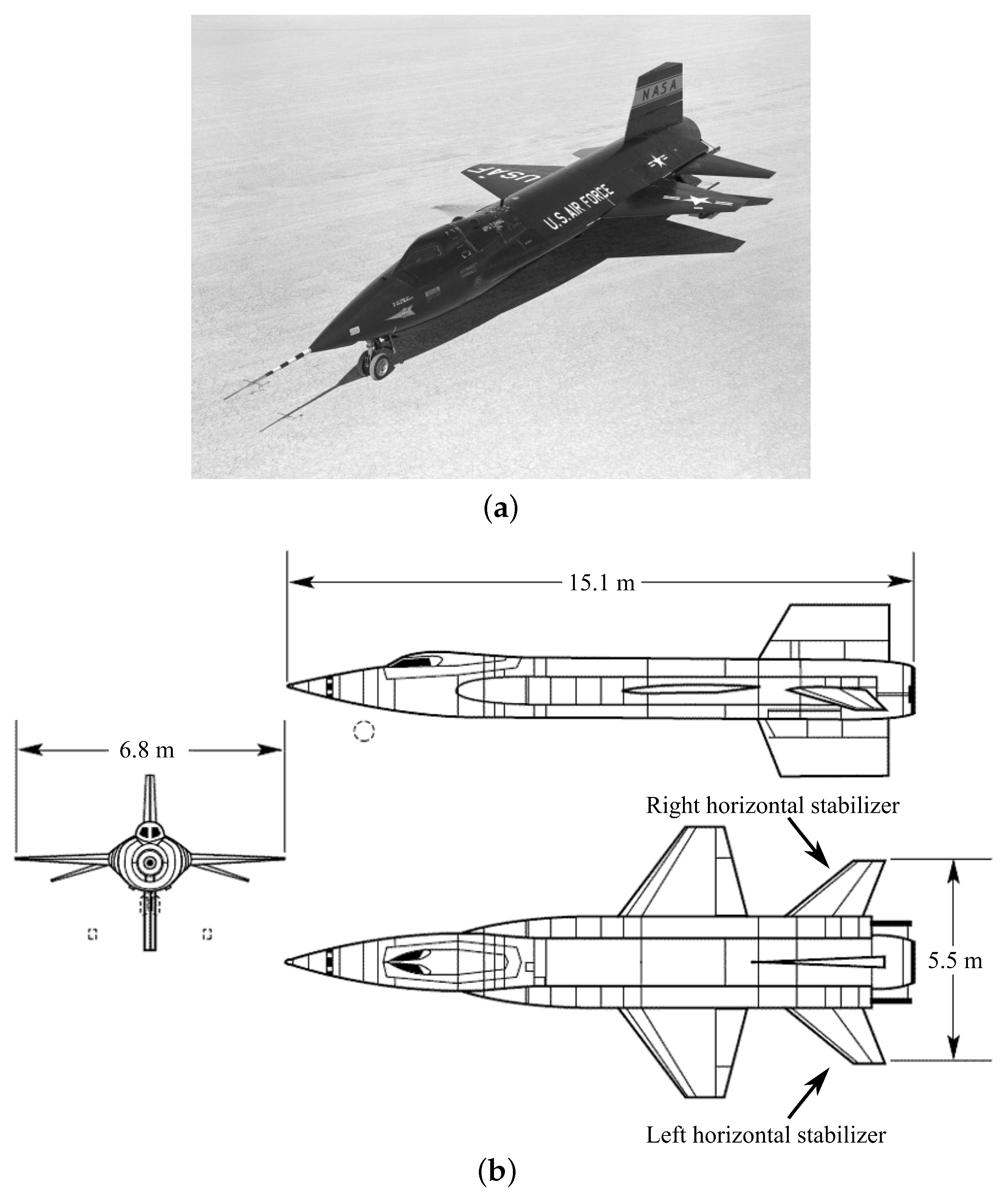
To perform the numerical simulations of the controlled flight, the rocket-powered X-15 aircraft (North American Aviation, Inc., Los Angeles, CA, USA) (Figure 1) was used as a test platform. The original X-15 aircraft was equipped with two elevators that can be deflected independently. The roll angle was controlled by the differential elevator deflections. The real X-15 initially was also equipped with two liquid-propellant Reaction Motors XLR11 (Reaction Motors Inc., Denville, NJ, USA) that could produce a total 71 kN thrust. Later, these engines were replaced by a single XLR99 motor (Reaction Motors Division of Thiokol Chemical Corporation, Denville, NJ, USA) with a 250 kN thrust.

For the presented study, several assumptions were made. The model of the first version of the propulsion system was used. It was assumed that the main motor operational duration is 180 s with a maximum thrust magnitude of 71 kN. In that way, for the purposes of the presented study, it was assumed that the maximum possible speed during the controlled flight was approximately up to Mach number 2. For the analysis, it was assumed that pitch and yaw angles are influenced using only the deflectable engine nozzle. The maximum nozzle deflection angles and elevators’ deflections were set to ±15${}^{\circ }$ [41]. For the original X-15, the minimum turn radius was approximately 66 km, and, based on that, the maximum allowed lateral load was 4 g. The data from [41,42] were used as input parameters for the vehicle model.

Table 1. X-15 experimental aircraft data.

Parameter	Symbol	Value	Unit	Source
Mass (zero fuel)	$m_0$	7057.89	$\mathrm{kg}$	[42]
Moment of inertia (zero fuel)	$I_{xx0}$	4948.74	$\mathrm{kg}·{\mathrm{m}}^2$	[42]
Moment of inertia (zero fuel)	$I_{yy0}$	108,465.44	$\mathrm{kg}·{\mathrm{m}}^2$	[42]
Moment of inertia (zero fuel)	$I_{zz0}$	111,177.07	$\mathrm{kg}·{\mathrm{m}}^2$	[42]
Product of inertia (zero fuel)	$I_{xz0}=I_{zx0}$	799.93	$\mathrm{kg}·{\mathrm{m}}^2$	[42]
Mass (at launch)	$m_f$	25,849.50	$\mathrm{kg}$	[43]
Moment of inertia (at launch)	$I_{xxf}$	18,127.01	$\mathrm{kg}·{\mathrm{m}}^2$	Estimated
Moment of inertia (at launch)	$I_{yyf}$	397,302.82	$\mathrm{kg}·{\mathrm{m}}^2$	Estimated
Moment of inertia (at launch)	$I_{zzf}$	407,237.03	$\mathrm{kg}·{\mathrm{m}}^2$	Estimated
Product of inertia (at launch)	$I_{xzf}=I_{zxf}$	2930.11	$\mathrm{kg}·{\mathrm{m}}^2$	Estimated
Mean aerodynamic chord	$\overline{c}$	3.13	$\mathrm{m}$	[41,42]
Wing span	b	6.81	$\mathrm{m}$	[41,42]
Reference area	$S_{ref}$	18.58	${\mathrm{m}}^2$	[41,42]
Aspect ratio	$\mathrm{\Lambda }$	2.5	-	[41,42]
Oswald efficiency number	e	0.9	-	Estimated

contains the necessary mass properties and reference parameters of the X-15 aircraft.

It was assumed that the aircraft is equipped with external fuel tanks to ensure 180 s of operation of the main motor.

3. Flight Simulation Model

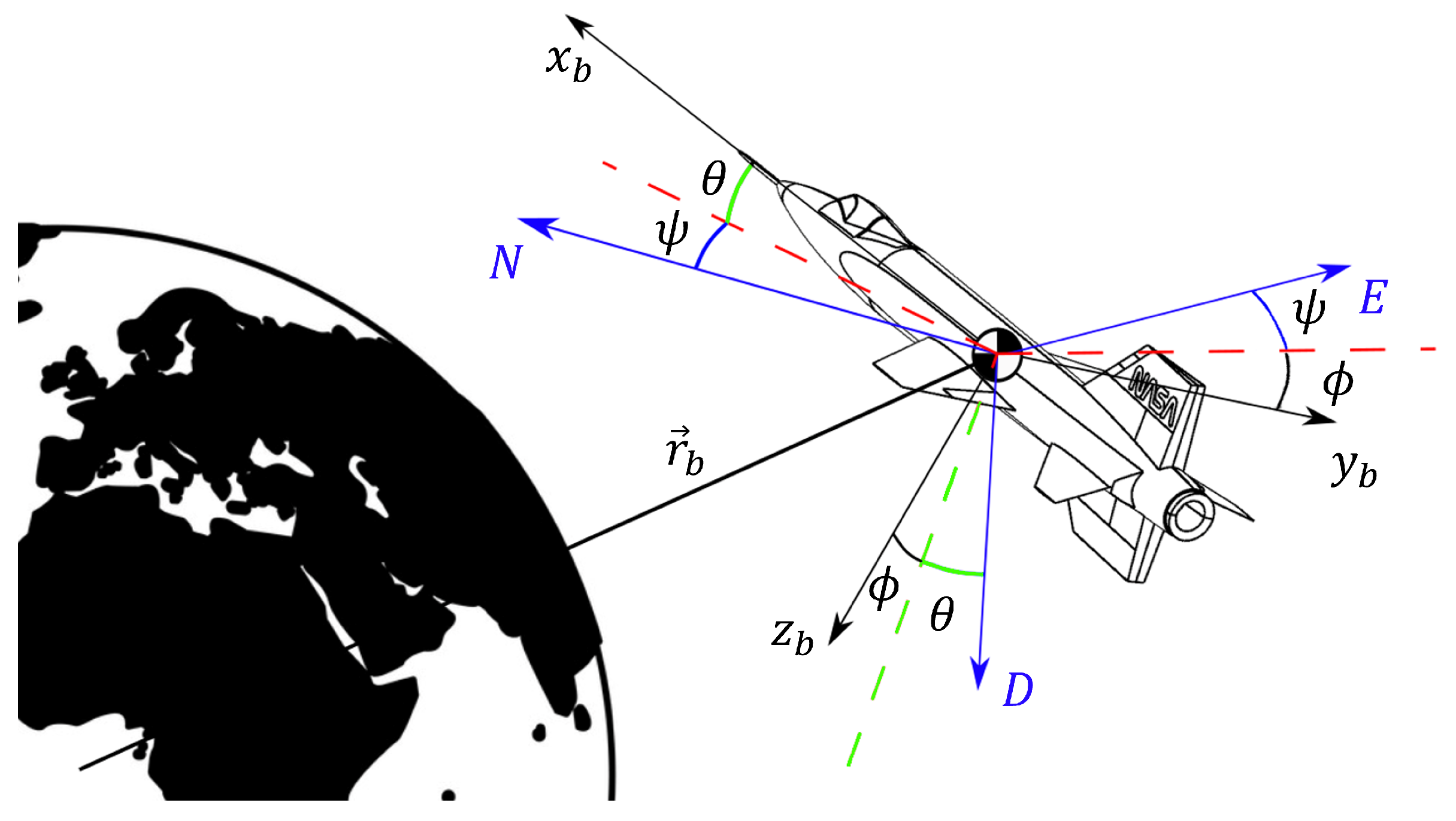
The MATLAB/Simulink six degrees of freedom (DOF) Earth-centred Earth-fixed (ECEF) quaternion-based nonlinear mathematical model was used. This model describes the equations of motion with respect to a rotating ECEF frame of reference [44]. These equations of motion are solved with respect to the center of mass of the object, which is assumed to be rigid [45]. Meanwhile, the Euler angles $\varphi$, $\theta$, $\psi$ that describe the orientation of the body-fixed frame $O_b{x}_b{y}_b{z}_b$ in space are defined with respect to a gravity coordinate system $O_g{x}_g{y}_g{z}_g$ (See Figure 2). For further simplification, the mass and inertia of the object are assumed to be constants. The sum of forces and moments (evaluated with respect to the center of mass) are described by Equations (1) and (2).

$$m({\overrightarrow{\dot{V}}}_b+{\overrightarrow{\omega }}_b\times {\overrightarrow{V}}_b+C_E^B{\overrightarrow{\omega }}_e\times {\overrightarrow{V}}_b+C_E^B\times ({\overrightarrow{\omega }}_e\times ({\overrightarrow{\omega }}_e\times {\overrightarrow{r}}_b)))=F_A+F_G+F_T$$

(1)

$$I{\overrightarrow{\dot{\omega }}}_b+{\overrightarrow{\omega }}_b\times \left(I{\overrightarrow{\omega }}_b\right)=M_A+M_T$$

(2)

where:

m—Aircraft mass;

${\overrightarrow{\dot{V}}}_b$—Linear acceleration vector in the body coordinate system;

${\overrightarrow{\omega }}_b$—Angular velocity vector in the body coordinate system;

${\overrightarrow{\omega }}_e$— Earth’s angular velocity vector;

${\overrightarrow{V}}_b$—Velocity vector in the body coordinate system;

${\overrightarrow{r}}_b$—Aircraft position vector in the Earth-centered Earth-fixed frame;

${\overrightarrow{\dot{\omega }}}_b$—Angular acceleration vector in the body coordinate system;

$C_E^B$—Transformation matrix from Earth-centered Earth-fixed frame to the body coordinate system;

I—Mass moment of inertia tensor with respect to the center of mass;

$F_A$—Aerodynamic force vector;

$F_G$—Gravitational force vector;

$F_T$—Thrust force vector;

$M_A$—Aerodynamic moment vector;

$M_T$—Thrust moment vector.

Figure 2. Body-fixed coordinate system $O_b{x}_b{y}_b{z}_b$, gravity coordinate system $O_g{x}_g{y}_g{z}_g$, and attitude angles.

Figure 2. Body-fixed coordinate system $O_b{x}_b{y}_b{z}_b$, gravity coordinate system $O_g{x}_g{y}_g{z}_g$, and attitude angles.

The Coriolis effect plays a significant role and is expressed in Equation (1) by terms ${\overrightarrow{\omega }}_b\times {\overrightarrow{V}}_b+C_E^B{\overrightarrow{\omega }}_e\times {\overrightarrow{V}}_b$. This is an apparent force, and in the Northern Hemisphere it tries to deflect the trajectory of the moving object to the right. In that way, the object has a tendency to drift sideways from the nominal direction.

The gravitational acceleration was assumed to be constant ($g=9.81$$\mathrm{m}/{\mathrm{s}}^2$) in the NED (North-East-Down) frame of reference. The gravitational loads in the body-fixed frame are described by Equation (3).

$$F_G=\left[\begin{array}{c}-mg\sin \left(\theta \right)\\ mg\cos \left(\theta \right)\sin \left(\varphi \right)\\ mg\cos \left(\theta \right)\cos \left(\varphi \right)\end{array}\right]$$

(3)

Accurate modeling of aerodynamic forces and moments is crucial for simulations of aerospace vehicles. The aerodynamic model utilized in the study incorporates features of aerodynamic incidence angles’ periodicity and the effects of control surfaces on the projectile. For this study, the effects of control surfaces have been included; however, the model has been simplified to include the most crucial aspects of aerodynamic forces (see Equation (4)) and moments (see Equation (5)) in the conducted analysis.

$$F_A={\displaystyle \frac{1}{2}}\rho v_A^2{S}_{ref}\left({\mathbf{C}}_A^B\left[\begin{array}{c}-C_D\\ C_S\\ -C_L\end{array}\right]\right)$$

(4)

$$M_A={\displaystyle \frac{1}{2}}\rho v_A^2{S}_{ref}\left(\left[\begin{array}{c}b\times C_l\\ \overline{c}\times C_m\\ b\times C_n\end{array}\right]\right)$$

(5)

where:

$\rho$—Air density;

$S_{ref}$—Reference area;

$v_A$—Aircraft’s velocity magnitude relative to the airflow;

${\mathbf{C}}_A^B$—Transformation matrix from aerodynamic to body frame;

$C_i$—Coefficients of drag, side force, lift and rolling, pitching and yawing moments for $i=D,S,L,l,m,n$, respectively,

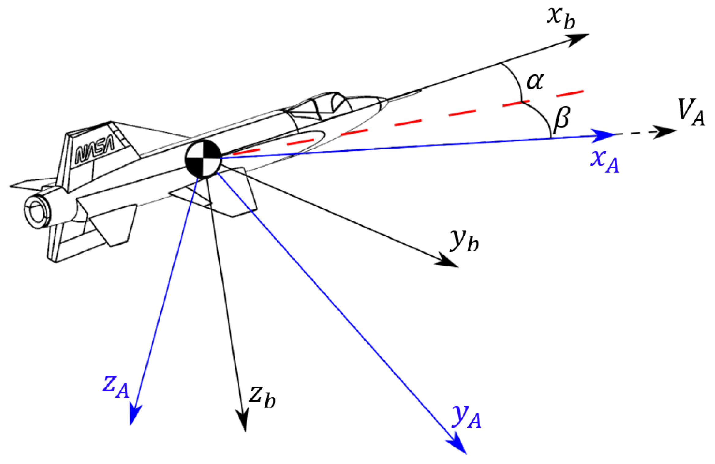
The relationship between the body frame $O_b{x}_b{y}_b{z}_b$ and the aerodynamic frame $O_A{x}_A{y}_A{z}_A$ with the definition of the aerodynamic incidence angles and the vectors of aerodynamic loads was presented in Figure 3. The transformation matrix from the aerodynamic frame to the body frame can be observed in Equation (6) in addition to Equations (7) and (8), which define the angle of attack $\alpha$ and slide slip angle $\beta$ obtained from [46].

$$C_A^F=\left[\begin{array}{ccc}\cos \left(\alpha \right)\cos \left(\beta \right)& -\cos \left(\alpha \right)\sin \left(\beta \right)& -\sin \left(\alpha \right)\\ \sin \left(\beta \right)& \cos \left(\beta \right)& 0\\ \sin \left(\alpha \right)\cos \left(\beta \right)& -\sin \left(\alpha \right)\sin \left(\beta \right)& \cos \left(\alpha \right)\end{array}\right]$$

(6)

$$\alpha =\arctan \left({\displaystyle \frac{V_{b_3}}{V_{b_1}}}\right)$$

(7)

$$\beta =\arcsin \left({\displaystyle \frac{V_{b_2}}{|V_b|}}\right)$$

(8)

The total aerodynamic coefficients of the X-15 hypersonic vehicle were obtained through reports found in [42]. These coefficients depend on various variables such as the Reynolds number, Mach number, incidence angles, surface roughness, etc. A common approach in the field of aerodynamics is to analyze nondimensional aerodynamic coefficients; this provides a clearer understanding of vehicle performance. The total coefficients are comprised of derivative coefficients that are Mach number dependent, and the non-dimensional aerodynamic coefficients utilized in the aerodynamic model were defined in Equations (9)–(14).

$$C_D=C_{D0}\left(M\right)+{\displaystyle \frac{C_L^2}{e\mathrm{\Lambda }\pi }}$$

(9)

$$C_Y=C_{Y_{\beta }}\left(M\right)\beta +C_{y_{\delta a}}\left(M\right){\delta }_a$$

(10)

$$C_L=C_{L0}\left(M\right)+C_{L_{\alpha }}\left(M\right)\alpha$$

(11)

$$C_l=C_{l_{\beta }}\left(M\right)\beta +C_{l_p}\left(M\right)\frac{bp}{2v_A}+C_{l_r}\left(M\right)\frac{br}{2v_A}+C_{l_{{\delta }_a}}\left(M\right){\delta }_a$$

(12)

$$C_m=C_{m_{\alpha }}\left(M\right)\alpha +C_{m_q}\left(M\right)\frac{\overline{c}q}{2v_A}+C_{m_{\dot{\alpha }}}\left(M\right)\frac{\overline{c}\dot{\alpha }}{2v_A}$$

(13)

$$C_n=C_{n_{\beta }}\left(M\right)\beta +C_{n_p}\left(M\right)\frac{bp}{2v_A}+C_{n_r}\left(M\right)\frac{br}{2v_A}+C_{n_{{\delta }_a}}\left(M\right){\delta }_a$$

(14)

where:

M—Mach number;

${\delta }_a$—Aileron deflection angle;

p—Rolling angular rate;

q—Pitching angular rate;

r—Yawing angular rate;

$\dot{\alpha }$—Angle of attack derivative.

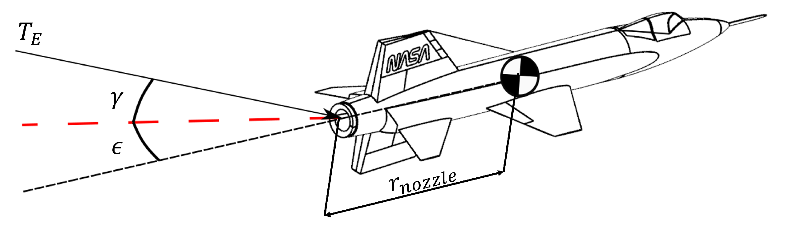
For the purpose of this study, the thrust generated by the X-15 aircraft was assumed to be a constant magnitude of 71 kN ($T_E$) for 180 s of motor operation. The deflection angles of the thrust vector $\gamma$ (in pitch plane $O_b{x}_b{z}_b$) and $ϵ$ (in yaw plane $O_b{x}_b{y}_b$) are defined in Figure 4. The components of the thrust force $F_T$ and the torque $M_T$ generated by this force are defined by Equations (15) and (21). The distance between the center of the mass of the aircraft and the nozzle $r_{nozzle}$ was assumed to be 6 m.

$$F_T=\left[\begin{array}{c}{T}_E\cos \left(\gamma \right)\cos \left(ϵ\right)\\ T_E\sin \left(ϵ\right)\\ T_E\sin \left(\gamma \right)\end{array}\right]$$

(15)

$$M_T=\left[\begin{array}{c}{r}_{nozzle}\\ 0\\ 0\end{array}\right]\times F_T=\left[\begin{array}{c}0\\ -r_{nozzle}{T}_E\sin \left(\gamma \right)\\ r_{nozzle}{T}_E\sin \left(ϵ\right)\end{array}\right]$$

(16)

The International Standard Atmosphere (ISA) was utilized for computing the static pressure, temperature, air density, and speed of sound for the respective flight altitude. Equations (17)–(20) were used to define atmospheric parameters based on [47].

$$\rho \left(H\right)={\displaystyle \frac{p\left(H\right)}{RT\left(H\right)}}$$

(17)

$$p\left(H\right)=p_0{e}^{-{\displaystyle \frac{g}{R{T}_0}}(H-H_0)}$$

(18)

$$T\left(H\right)=T_0+L_0(H-H_0)$$

(19)

$$a\left(H\right)=\sqrt{kRT\left(H\right)}$$

(20)

where:

H—Geopotential altitude;

$H_0$—Reference altitude;

$T\left(H\right)$—Ambient temperature at the altitude H;

$T_0$—Ambient temperature at the altitude $H_0$;

$L_0$—Temperature gradient above $H_0$;

$p_0$—Pressure at $H_0$;

g—Gravitational acceleration;

R—Gas constant of air;

$\rho \left(H\right)$—Air density at the altitude H;

$a\left(H\right)$—Speed of sound at the altitude H;

k—Specific heat ratio.

4. Guidance Navigation and Control

The study assumed that the object should fly along a predefined trajectory in an autonomous mode. The trajectory for each flight scenario was defined by a set of waypoints. These waypoints were specified by the system’s user taking into account the performance limitations of the object.

4.1. Waypoint Guidance

Guidance logic developed by Park et al. [48] was adopted in this study. This algorithm requires a list of waypoints as inputs and several parameters. The outputs are the three coordinates of the lookahead point and the commanded yaw angle. The minimum lookahead distance was set to 400 m and the acceptance radius of the waypoint was 100 m.

4.2. Autopilot Control Algorithm

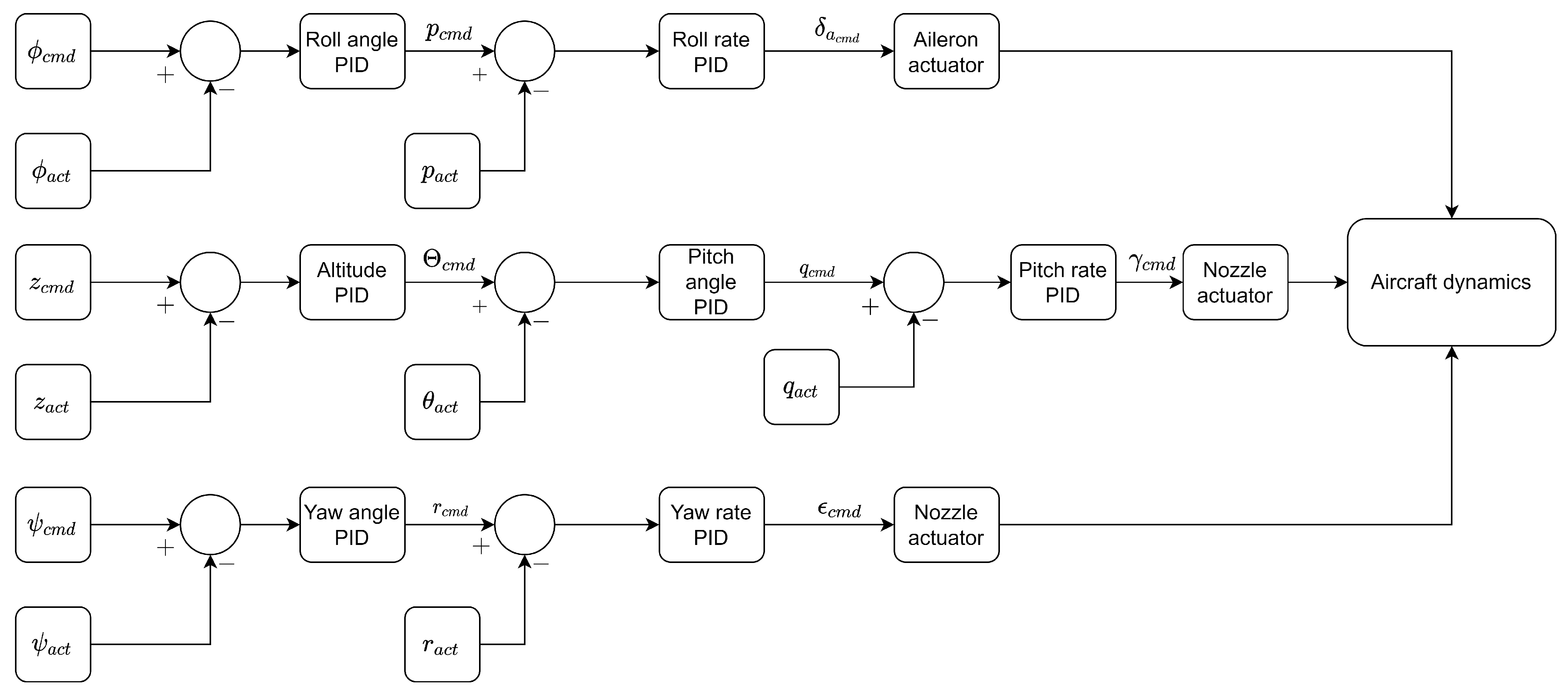
The autopilot control algorithm output signal comprises three control channels: roll control channel, pitch control channel, and yaw control channel. The roll control channel outputs the desired differential elevators’ deflection angle in order to ensure a roll stabilization; this was the sole requirement for this control channel. Furthermore, the pitch channel outputs the desired nozzle deflection angle $\gamma$ in the $O_b{x}_b{z}_b$ plane; this causes the aircraft to pitch. On the other hand, the yaw control channel outputs the desired nozzle deflection angle $ϵ$ in the $O_b{x}_b{y}_b$ plane, causing the aircraft to yaw. The inputs to the pitch and yaw control channels are the desired altitude change and the desired heading, which are computed by the guidance algorithm, respectively. PID (proportional–integral–derivative) controllers were utilized for all autopilot channels; Figure 5 present the autopilot schematics for each control channel. Additionally, it should be noted that the elevators and nozzle deflection actuators were modeled using first-order transfer functions:

$$\frac{\gamma \left(s\right)}{{\gamma }_c\left(s\right)}=\frac{1}{T_{\gamma }s+1}$$

(21)

$$\frac{ϵ\left(s\right)}{{ϵ}_c\left(s\right)}=\frac{1}{T_{ϵ}s+1}$$

(22)

where:

${\gamma }_c$—Commanded nozzle deflection angle in $O_b{x}_b{z}_b$ plane;

${ϵ}_c$—Commanded nozzle deflection angle in $O_b{x}_b{y}_b$ plane;

$T_{\gamma },T_{ϵ}$—Time constants.

The values of $T_{\gamma }$ and $T_{ϵ}$ were obtained by the analysis of existing real systems and assumed to be equal to 0.5 $\mathrm{s}$.

Figure 5. Autopilot structure.

Figure 5. Autopilot structure.

5. Mission Plan

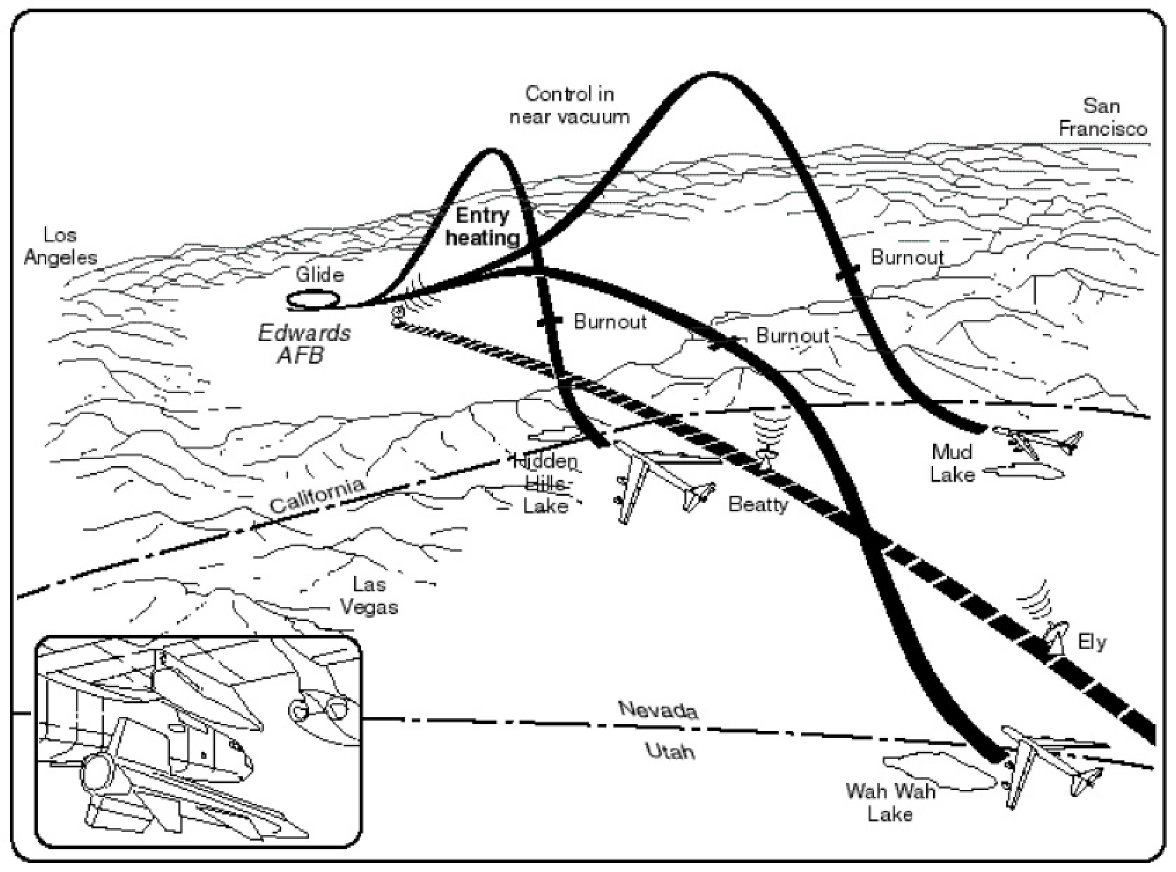
The X-15 aircraft was designed as a result of the space race during the twentieth century to overcome the tremendous challenge of designing such an experimental vehicle. The pursuit of designing a vehicle capable of reaching the edge of space to push the boundaries of human understanding into the hypersonic flow regime and fly past the 100 km of altitude led to this project by NASA. The main goal of the X-15 program was for NASA to aid in the development of materials capable of surviving the heat of reentry and the structures required for the stability and handling of the aircraft during hypersonic flight. The original mission plan of the X-15 plan involved releasing the aircraft from a carrier vehicle, which was followed by igniting the rocket motors powered by liquid propellant. The aircraft then accelerated forward and pitched upwards to increase the flight altitude, where the experimentation took place (see Figure 6). Several flights of the X-15 aircraft took place during the program’s lifetime, with one flight achieving the record for the fastest manned mission of the time by reaching a Mach number of 6.7.

As mentioned above, this article investigated the use of thrust vector control with the aid of movable control surfaces to control the X-15 aircraft in the flight model. Several mission scenarios were considered to check the control performance under four various flight conditions. These are:

• Scenario 1—Uncontrolled flight.
• Scenario 2—The maneuvers were realized only in the pitch plane (similar to the original mission plan of the aircraft).
• Scenario 3—The maneuvers were realized only in the yaw plane and the skid-to-turn method was used to change the flight direction.
• Scenario 4—Couples’ pitch and yaw maneuvers using skid-to-turn strategy (the same as in scenario 3).
• Scenario 5—Couples’ pitch and yaw maneuvers but the aircraft used the bank-to- turn strategy.

6. Results

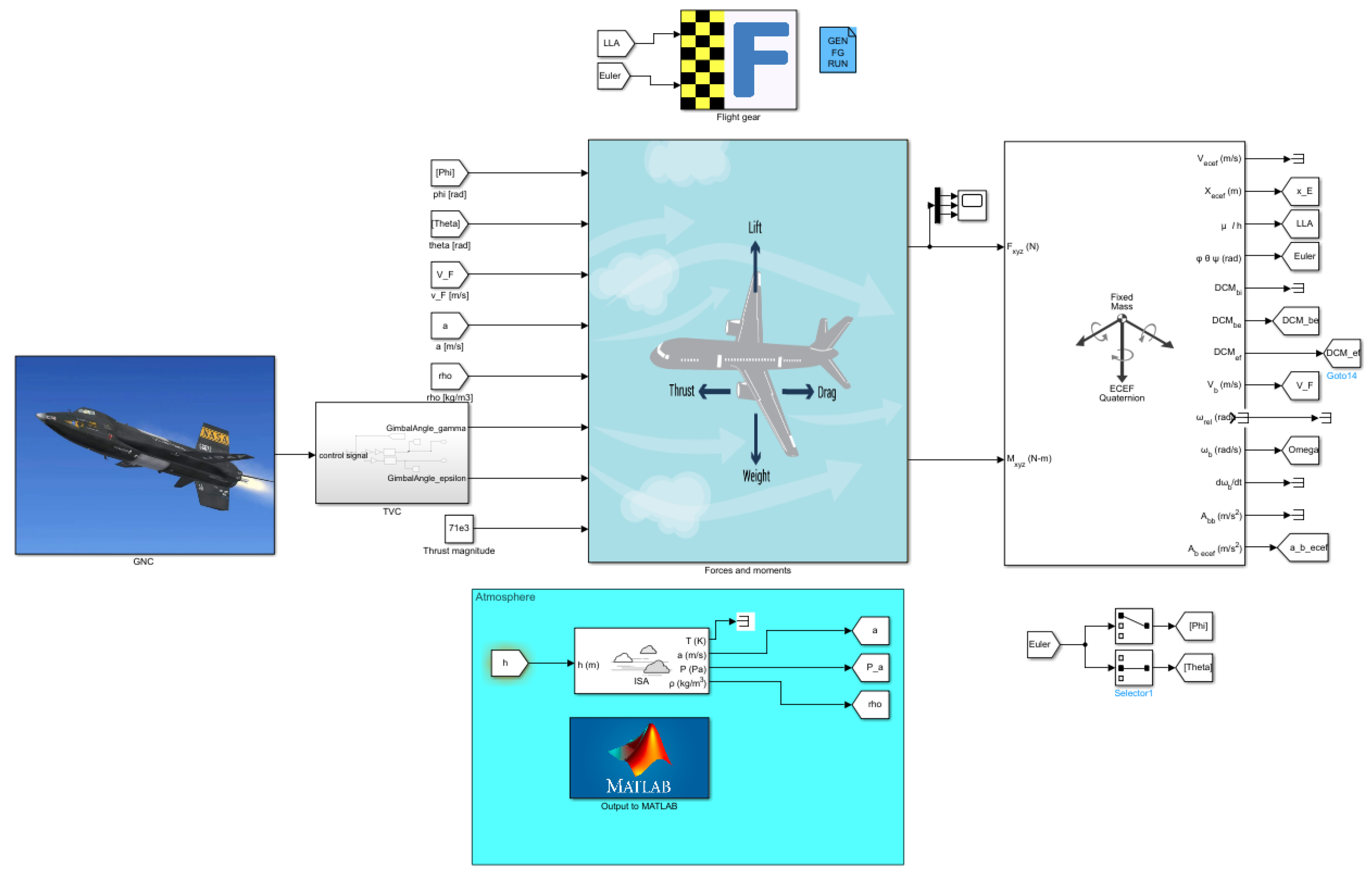
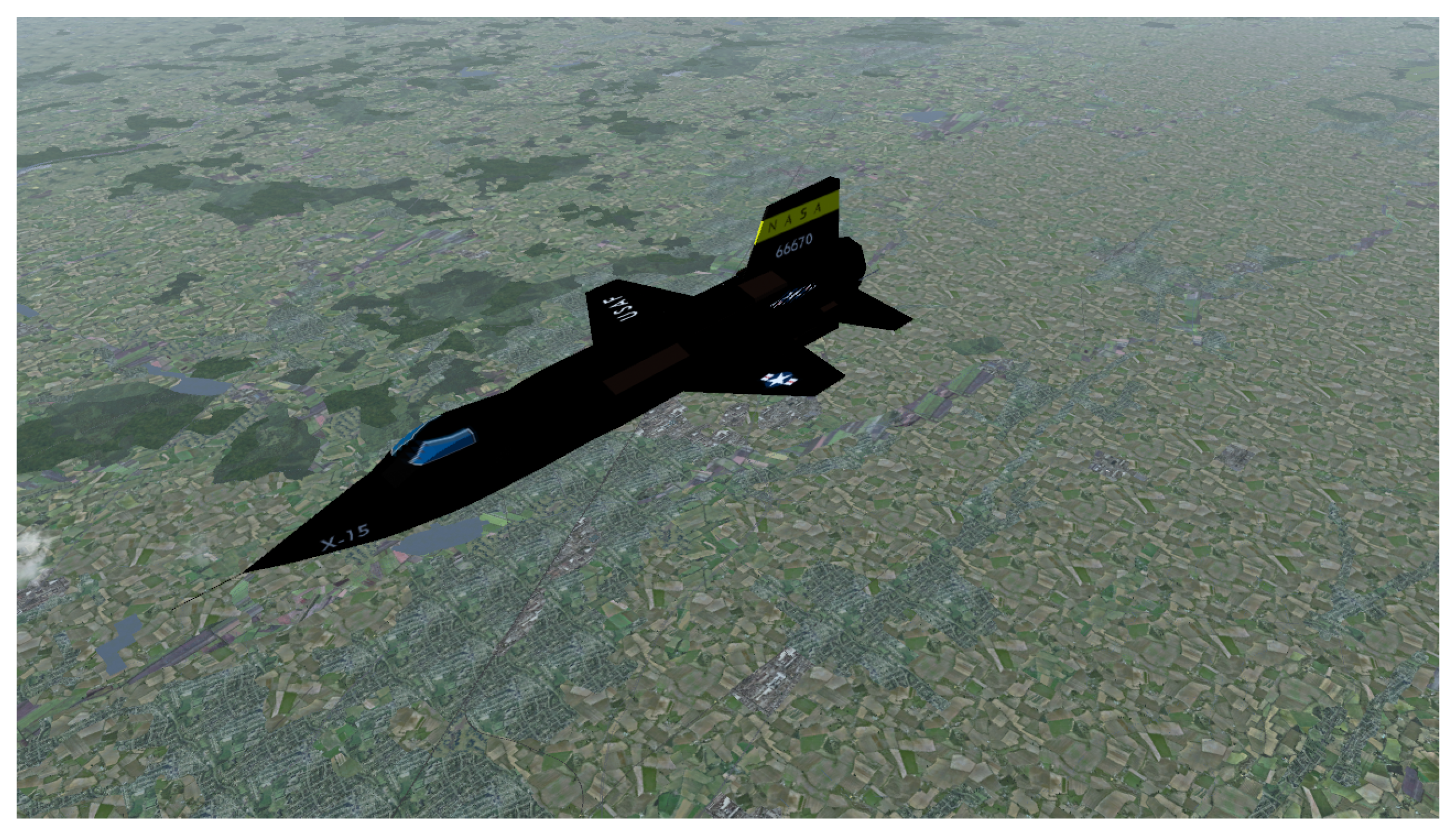
The developed model was implemented in a MATLAB/Simulink 2022a environment (see model schematics in Figure 7). The equations of motion were solved using the Runge-Kutta (RK4)-fixed step solver with step time 0.0005 s, with a total simulation time set to 180 s. To decrease the complexity of the analysis, no sensors were modelled, and the flight parameters obtained from the equations of motion were directly used in the guidance and control algorithms. The model was interfaced with FlightGear to visualise the aircraft motion (Figure 8).

The initial conditions for all simulation scenarios can be found in

Table 2. Simulation’s initial conditions.

Parameter	Value	Unit
Latitude	52.26	${}^{\circ }$
Longitude	20.91	${}^{\circ }$
Altitude	10,000	$\mathrm{m}$
$V_0$	270	$\mathrm{m}/\mathrm{s}$
${\varphi }_0$	0	${}^{\circ }$
${\theta }_0$	0	${}^{\circ }$
${\psi }_0$	90	${}^{\circ }$
$p_0=q_0=r_0$	0	${}^{\circ }/\mathrm{s}$

.

6.1. Scenario 1

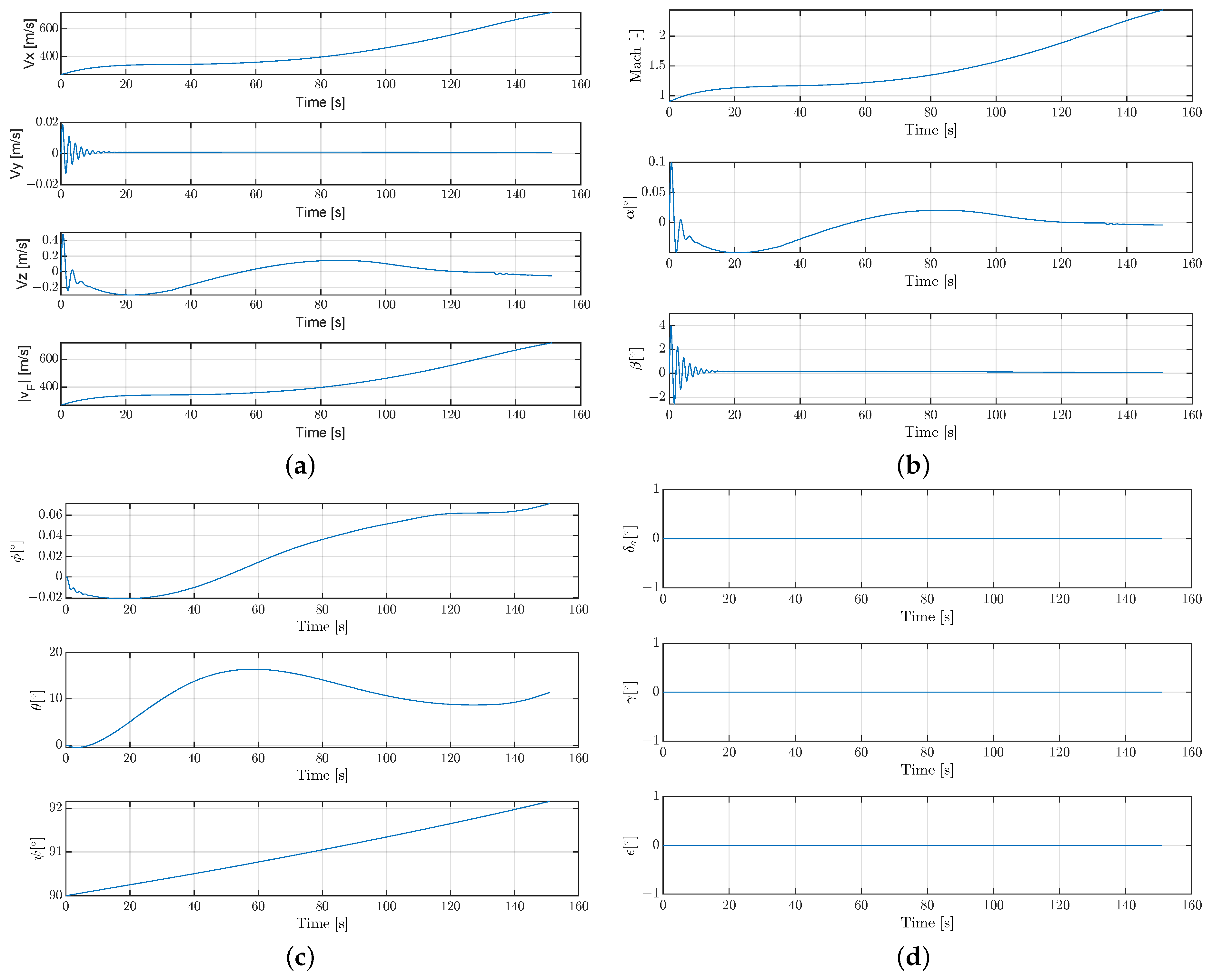
As previously mentioned, in scenario 1, the aircraft was able to perform an uncontrolled flight. The TVC system was deactivated and not used to influence the aircraft trajectory. That means the nozzle angles $\gamma$ and $ϵ$ were equal to 0${}^{\circ }$. In Figure 9a, the components of the aircraft velocity vector and the velocity magnitude were presented. In Figure 9b, the Mach number, angle of attack, and sideslip were illustrated. Meanwhile, in Figure 9c, the aircraft Euler angles were shown. Finally, the nozzle deflection angles were presented in Figure 9d.

The velocity of the aircraft rose during the flight until it reached a maximum value of ≈700 $\mathrm{m}/\mathrm{s}$, which was almost about Mach 2.5. The angle of attack and sideslip angles were approximately zero. A slight jump in the pitch angle was noticed; this can be explained by the aerodynamic characteristics of the aircraft and the effects from Coriolis forces. While both nozzle deflection angles were equal to 0${}^{\circ }$ because the thrust vectoring was not used in the presented scenario.

In the longitudinal aircraft response (Figure 9a, third subplot) it is possible to observe typical aircraft dynamic modes in the longitudinal motion: short period oscillations (with a period of approximately 1.98 s) and phugoid (with a period of 130 s). The same effects might be observed in changes of the angle of attack (Figure 9b, second subplot).

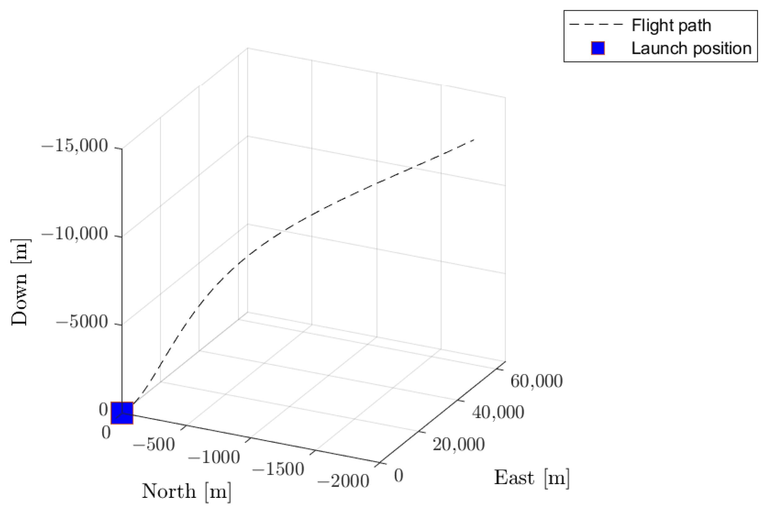
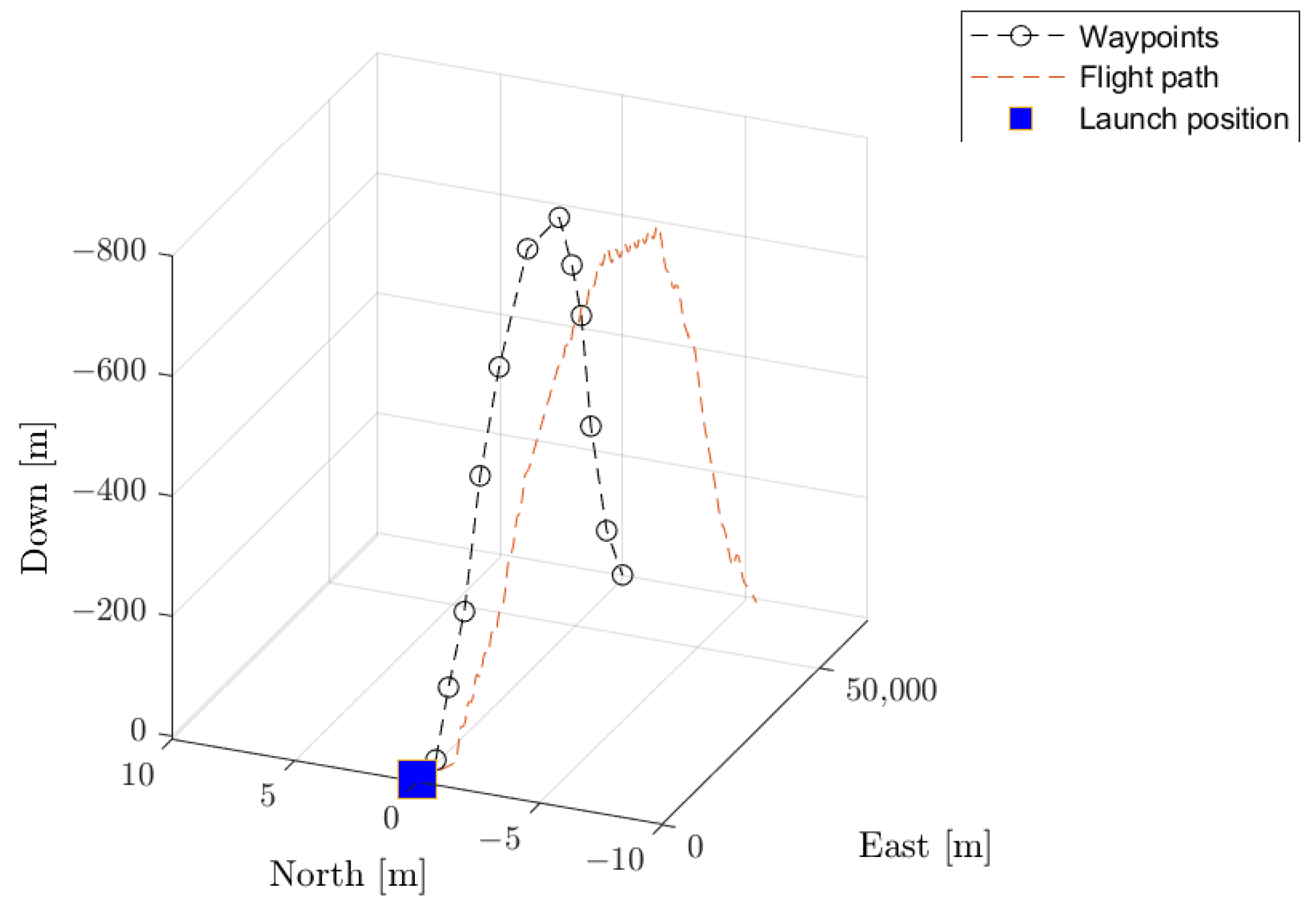
The three-dimensional trajectory is presented in Figure 10. On the vertical axis, the change in altitude (actual value–initial value) was shown.

It can be observed from the results that there is a large drift in the lateral and vertical directions; this occurs due to the Coriolis effects acting on the aircraft. This flight scenario took place in the northern hemisphere of the globe. However, if one runs the exact scenario in the southern hemisphere, the opposite drift in direction will happen. In addition, no drift will be observed while flying along the equator.

6.2. Scenario 2

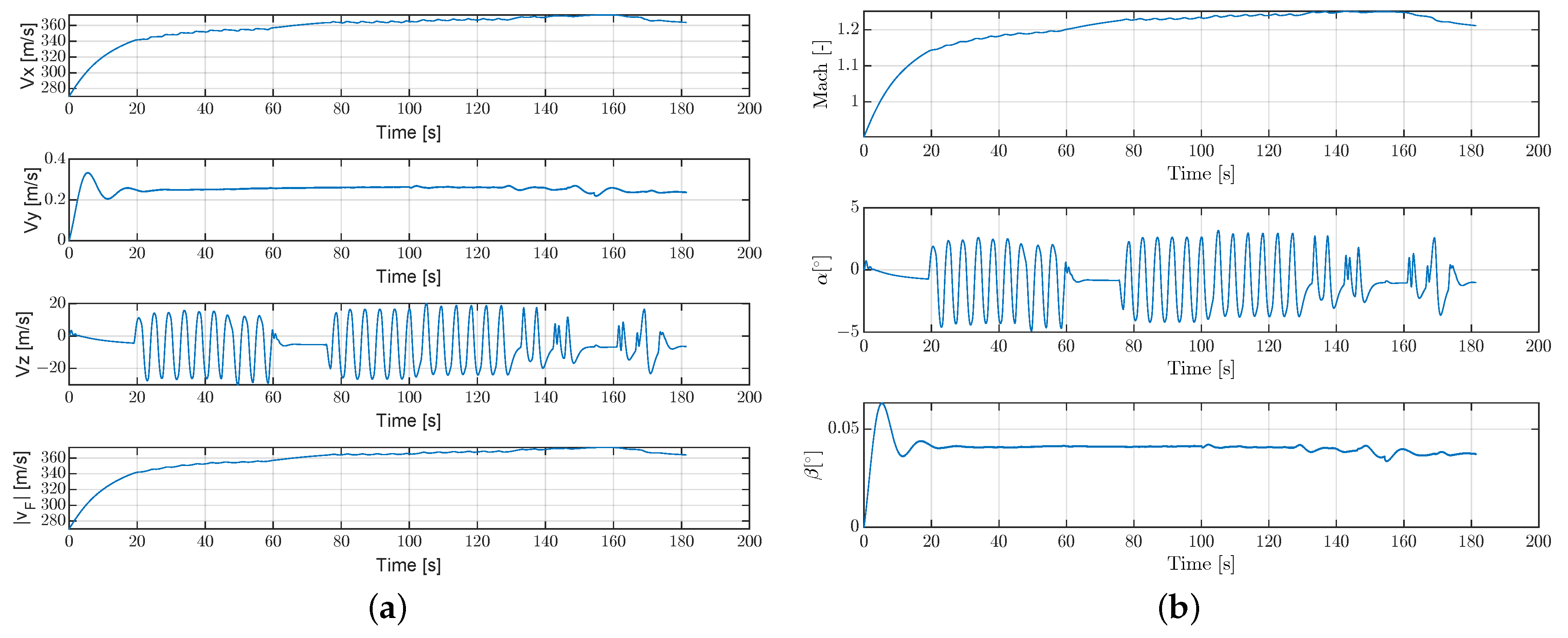
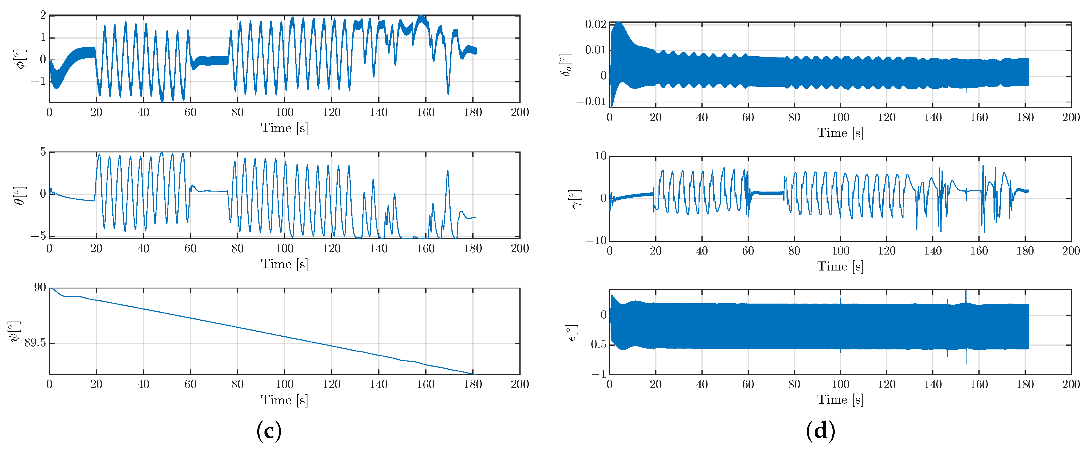
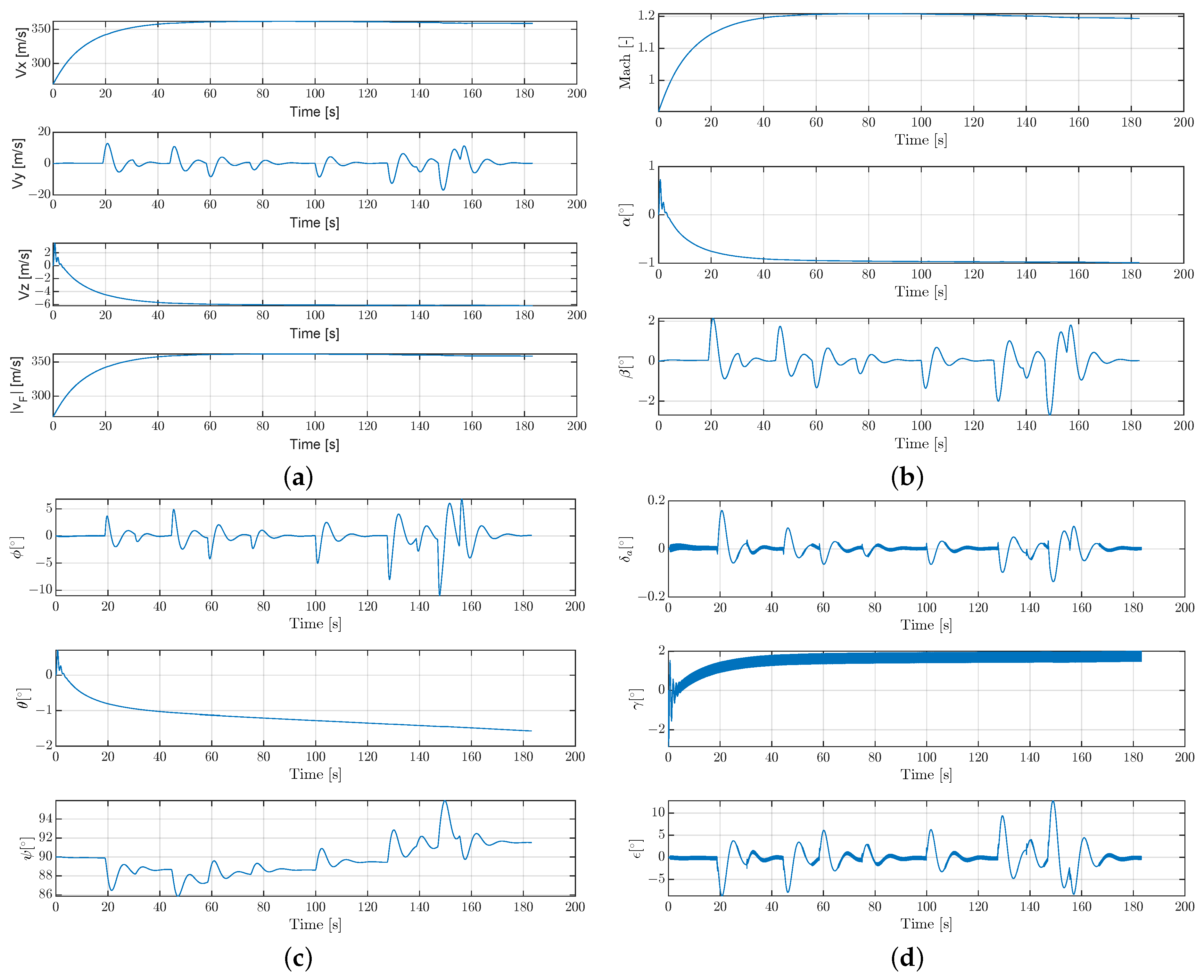
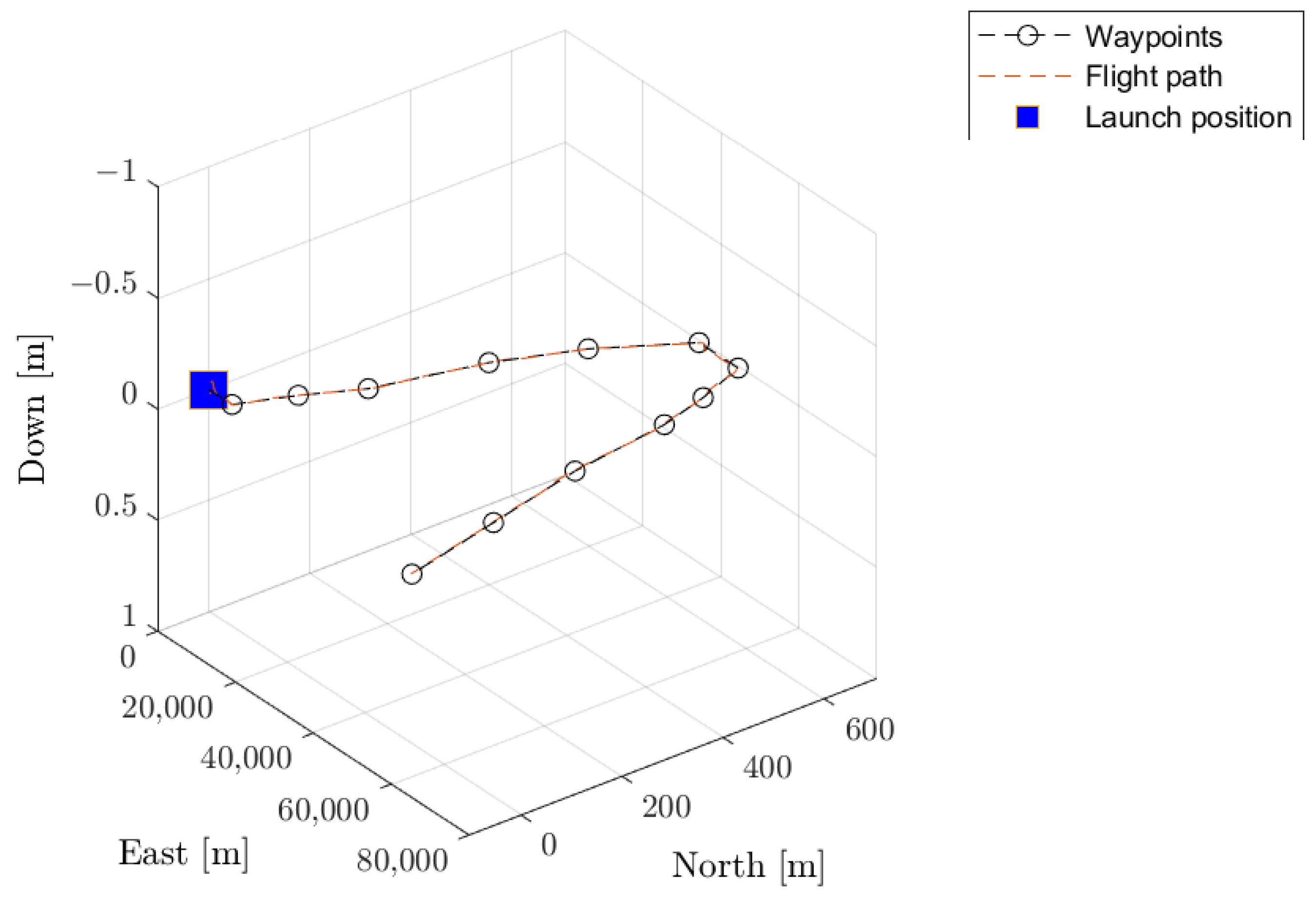
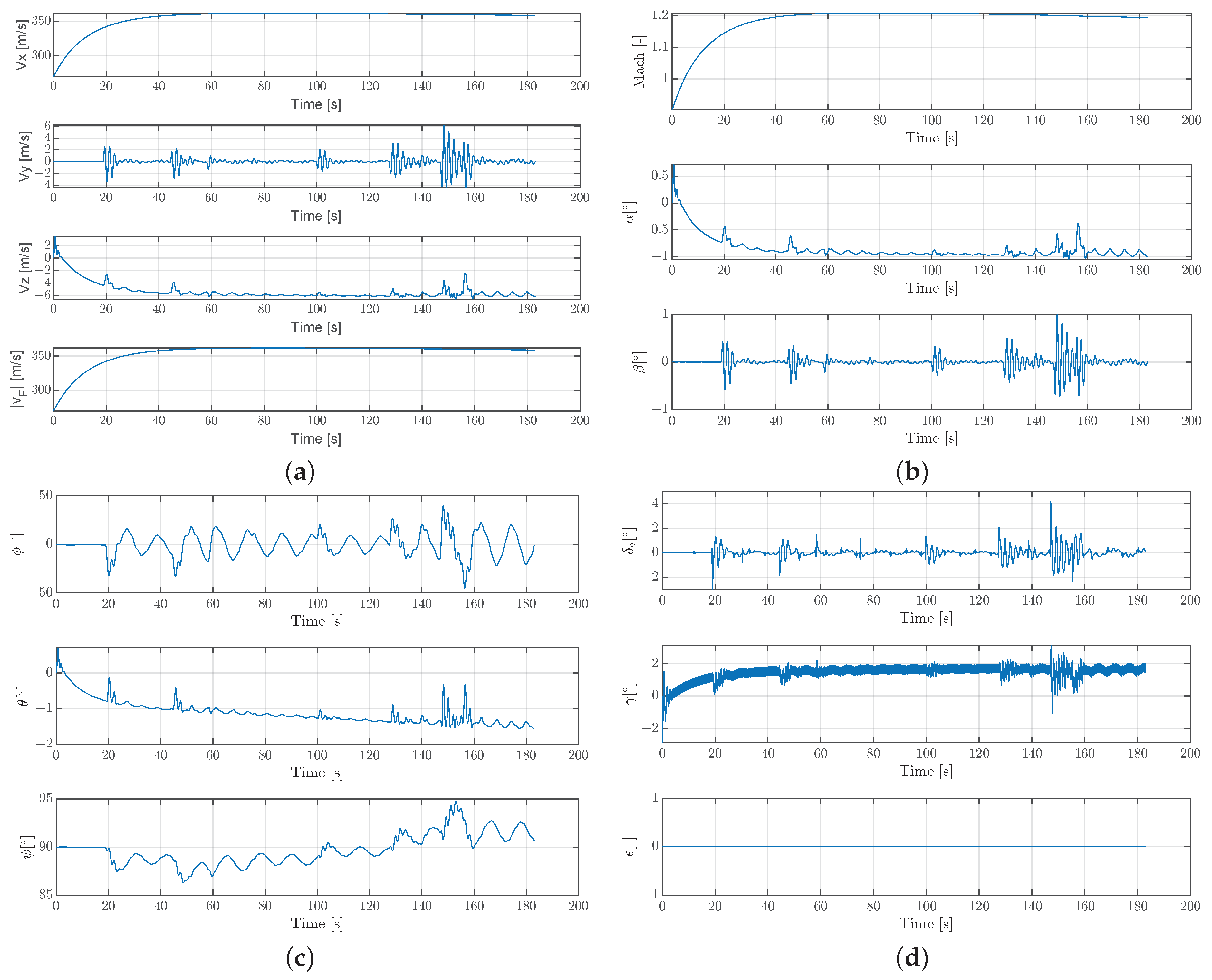
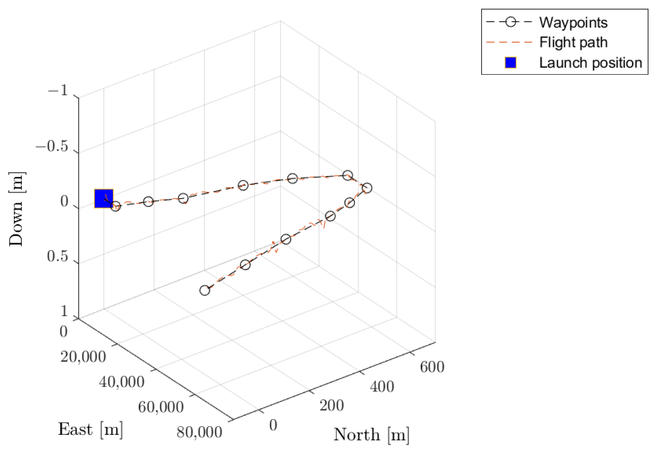
The simulations for the second scenario were then accomplished. The aircraft performed a set of maneuvers only in a vertical plane, similar to the original mission of the aircraft. The obtained results are presented in Figure 11 and Figure 12. This time, at the beginning of the flight, the aircraft velocity increased from 250 and up to 360 m/s (Figure 11a). Then, the velocity autopilot successfully holds the speed at a constant level. The angle of attack (Figure 11b) oscillated between −4${}^{\circ }$ and +2${}^{\circ }$. The angle of the sideslip is very small, below 0.1${}^{\circ }$, and changed smoothly. The roll angle (Figure 11c) was about 0${}^{\circ }$. Moreover, the autopilot in the pitch and yaw channels achieved the desired commands. Moreover, the nozzle deflection angle $\gamma$ in the pitch plane is much larger in magnitude when compared to the angle in the yaw plane $ϵ$ (Figure 11d). Some small oscillations were observed. In a real application, such chattering should be eliminated or at least minimized. Finally, the predefined path was tracked by the aircraft (Figure 12).

At the end of the flight, the lateral deviation from the nominal path is of the order of several meters. The influence of the Coriolis force was compensated by the control system in comparison to the uncontrolled mission. The nozzle deflection angle changed very rapidly in Figure 11d. This chattering phenomenon might complicate, in reality, the implementation of the mechanically actuated TVC for this particular object. However, on the other hand, the fluidic TVC theoretically allows for obtaining quite a fast response.

6.3. Scenario 3

In scenario 3, the maneuvers were performed only in the horizontal plane. The autopilot for the speed hold achieved its desired goal. The angle of attack decreased and after 40 s was equal to −1${}^{\circ }$. However, the angle of the sideslip changed in a smooth way between −2.5${}^{\circ }$ and +2${}^{\circ }$. The roll angle was negligible (Figure 13c). The pitch angle oscillated between −5${}^{\circ }$ and +5${}^{\circ }$. The yaw angle decreased slowly from 90${}^{\circ }$ to 89.3${}^{\circ }$. The chattering phenomena of the nozzle deflection angle occurred (Figure 13d). However, the amplitude of these oscillations is rather small. The control system followed the prespecified path accurately (Figure 14).

6.4. Scenario 4

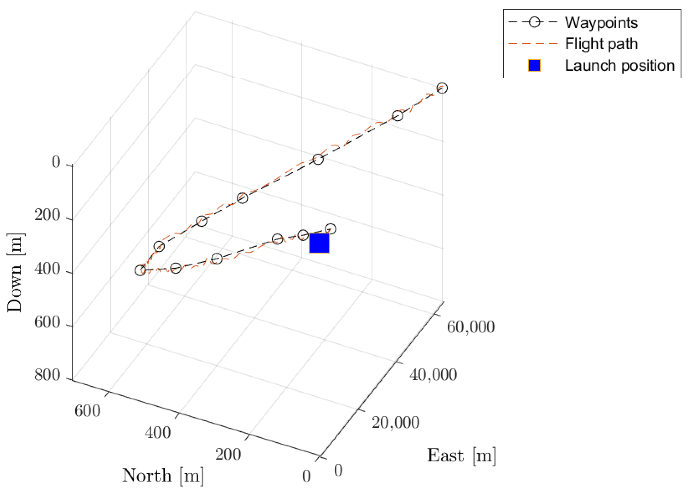
Scenario number 4 was more complicated than the previous cases, because this time the control was realized in the pitch and yaw plane simultaneously. The obtained results are shown in Figure 15a and Figure 16. The velocity hold autopilot was able to keep the aircraft speed (Figure 15a). Meanwhile, the angles of the attack and sideslip were in the same order and changed smoothly (Figure 15b).

The aircraft was able to fly along the prespecified path. The Coriolis effect influenced the vehicle trajectory, but the control system could successfully eliminate unintended drift from the nominal path. However, the aircraft’s configuration and low maneuverability introduced small oscillations to the trajectory.

6.5. Scenario 5

Scenario number 5 was the same as number 4, except that this time the aircraft used the bank-to-turn strategy instead of the skid-to-turn (as in scenarios from 1 to 4). The obtained results were presented in Figure 17 and Figure 18.

In scenario 5, the changes in the angle of attack (Figure 17b) are much less oscillatory when compared to scenario 4 (please see Figure 15b). The roll angle lies in the range from −50${}^{\circ }$ and up to +40${}^{\circ }$ (Figure 17c). The nozzle deflection angle $ϵ$ was equal to 0${}^{\circ }$ during the whole mission. The vehicle was able to precisely track the predefined path.

7. Conclusions

In this paper, the numerical flight simulation of the modified X-15 aircraft was shown. Several contributions of this paper were mentioned. The mathematical model of the hypersonic vehicle with the TVC and limited control authority was developed and implemented in MATLAB/Simulink. It was demonstrated that the thrust vectoring control can be used to achieve flight along the specified path for this aircraft, keeping in mind its nonstandard geometry. It should be noted that the X-15 aircraft was never designed to be maneuverable. The X-15 was used originally as a test platform to study physical phenomena in supersonic/hypersonic flow regimes and thermal effects. X-15 possesses rather low maneuverability characteristics. The large vertical tail dampens the yaw rate significantly when performing turns in the yaw plane. This fact, using the skid-to-turn method, might result in the chattering of the nozzle actuator. The developed control system is able to counteract the Coriolis effects (aircraft drift from the nominal trajectory). The original aircraft’s turn radius was estimated to be around 66 kilometers, which allows for lateral loads up to 4 g. Moreover, performing any set of complex maneuvers with tight turns with the modified version presented in the study results in increased loads on the structure and the pilot; this must be taken into account. Furthermore, increasing the speed of the aircraft will further deter performance, and the flight control systems will have a higher chance of failing to meet the desired mission objectives.

Further research should concentrate on including the sensor models in the developed simulation, building more complex actuator models, and introducing turbulence from wind effects on the presented mission profiles. In addition, more complicated mission scenarios might be considered.

References

- Flamm, J.; Deere, K.; Mason, M.; Berrier, B.; Johnson, S. Experimental Study of an Axisymmetric Dual Throat Fluidic Thrust Vectoring Nozzle for Supersonic Aircraft Application. In Proceedings of the 43rd AIAA/ASME/SAE/ASEE Joint Propulsion Conference and Exhibit, Cincinnati, OH, USA, 8–11 July 2007; pp. 2007–5084. [Google Scholar] [CrossRef] [Green Version]
- Wu, K.; Zhang, G.; Kim, T.H.; Kim, H.D. Numerical parametric study on three-dimensional rectangular counter-flow thrust vectoring control. Proc. Inst. Mech. Eng. Part G J. Aerosp. Eng. 2020, 234, 2221–2247. [Google Scholar] [CrossRef]
- Shin, C.S.; Kim, H.D.; Setoguchi, T.; Matsuo, S. A computational study of thrust vectoring control using dual throat nozzle. J. Therm. Sci. 2010, 19, 486–490. [Google Scholar] [CrossRef]
- Wu, K.; Kim, H.D.; Jin, Y. Fluidic thrust vector control based on counter-flow concept. Proc. Inst. Mech. Eng. Part G J. Aerosp. Eng. 2019, 233, 1412–1422. [Google Scholar] [CrossRef]
- Wu, K.; Kim, H. Fluidic Thrust Vector Control Using Shock Wave Concept. J. Korean Soc. Propuls. Eng. 2019, 23, 10–20. [Google Scholar] [CrossRef]
- Ferlauto, M.; Marsilio, R. Numerical Simulation of Fluidic Thrust-Vectoring. Aerotec. Missili Spaz. 2016, 95, 153–162. [Google Scholar] [CrossRef] [Green Version]
- Liu, J.F.; Luo, Z.B.; Deng, X.; Zhao, Z.J.; Li, S.Q.; Liu, Q.; Zhu, Y.X. Dual Synthetic Jets Actuator and Its Applications—Part II: Novel Fluidic Thrust-Vectoring Method Based on Dual Synthetic Jets Actuator. Actuators 2022, 11, 209. [Google Scholar] [CrossRef]
- Resta, E.; Marsilio, R.; Ferlauto, M. Thrust vectoring of a fixed axisymmetric supersonic nozzle using the shock-vector control method. Fluids 2021, 6, 441. [Google Scholar] [CrossRef]
- Wu, K.X.; Kim, T.H.; Kim, H.D. Numerical Study of Fluidic Thrust Vector Control Using Dual Throat Nozzle. J. Appl. Fluid Mech. 2021, 14, 73–87. [Google Scholar] [CrossRef]
- Liu, J.; Chen, Z.; Sun, M.; Sun, Q. Practical coupling rejection control for herbst maneuver with thrust vector. J. Aircr. 2019, 56, 1726–1734. [Google Scholar] [CrossRef]
- Zhou, Z.; Wang, Z.; Gong, Z.; Zheng, X.; Yang, Y.; Cai, P. Design of Thrust Vectoring Vertical/Short Takeoff and Landing Aircraft Stability Augmentation Controller Based on L1 Adaptive Control Law. Symmetry 2022, 14, 1837. [Google Scholar] [CrossRef]
- Dinca, L.; Corcau, J.I. Numerical study concerning longitudinal dynamic of a canard UAV with vectored thrust. In Proceedings of the 2021 International Conference on Applied and Theoretical Electricity, ICATE 2021, Craiova, Romania, 27–29 May 2021; pp. 1–5. [Google Scholar] [CrossRef]
- Raghavendra, P.K.; Sahai, T.; Kumar, P.A.; Chauhan, M.; Ananthkrishnan, N. Aircraft Spin Recovery, with and without Thrust Vectoring, Using Nonlinear Dynamic Inversion. J. Aircr. 2005, 42, 1492–1503. [Google Scholar] [CrossRef] [Green Version]
- Wu, Y.; Jiang, J.; Gu, C.; Li, T. Effect of thrust vectoring technology on taking-off performance of hypersonic vehicle. MATEC Web Conf. 2015, 31, 1–5. [Google Scholar] [CrossRef] [Green Version]
- Neely, A. Experimental Measurement of Fluidic Thrust Vectoring on Internal and External Expansion Hypersonic Nozzles; Technical Report AD1077648; Air Force Research Laboratory: Wright-Patterson, OH, USA, 2019. [Google Scholar]
- Li, B.; Dong, W.; Xiong, C. Robust Actuator-Fault-Tolerant Control System Based on Sliding-Mode Observer for Thrust-Vectoring Aircrafts. Asian J. Control 2019, 21, 236–247. [Google Scholar] [CrossRef]
- Lowenberg, M.H. Bifurcation analysis of multiple-attractor flight dynamics. Philos. Trans. R. Soc. A Math. Phys. Eng. Sci. 1998, 356, 2297–2319. [Google Scholar] [CrossRef]
- Mason, M.; Crowther, W. Fluidic Thrust Vectoring for Low Observable Air Vehicles. In Proceedings of the 2nd AIAA Flow Control Conference, Portland, OR, USA, 28 June–1 July 2004; pp. 2004–2210. [Google Scholar] [CrossRef]
- Skow, A.M. An analysis of the Su-27 flight demonstration at the 1989 Paris Airshow. SAE Tech. Pap. 1990, 99, 153–165. [Google Scholar] [CrossRef]
- Vinayagam, A.; Sinha, N. Optimal aircraft take-off with thrust vectoring. Aeronaut. J. 2013, 117, 1119–1138. [Google Scholar] [CrossRef]
- Sørensen, C.B.; Mosekilde, E.; Gránásy, P. Nonlinear dynamics of a vectored thrust aircraft. Phys. Scr. 1996, 1996, 176. [Google Scholar] [CrossRef]
- Ikaza, D.; Rausch, C. Thrust vectoring for eurofighter—the first steps. Air Space Eur. 2000, 2, 92–95. [Google Scholar] [CrossRef]
- Ikaza, D. Thrust Vectoring Nozzle for Military Aircraft Engines. In Proceedings of the 22nd Congress of International Council of the Aeronautical Sciences, Harrogate, UK, 27 August–1 September 2000; pp. 1–10. [Google Scholar]
- Páscoa, J.C.; Dumas, A.; Trancossi, M.; Stewart, P.; Vucinic, D. A review of thrust-vectoring in support of a V/STOL non-moving mechanical propulsion system. Cent. Eur. J. Eng. 2013, 3, 374–388. [Google Scholar] [CrossRef] [Green Version]
- Cen, Z.; Smith, T.; Stewart, P.; Stewart, J. Integrated flight/thrust vectoring control for jet-powered unmanned aerial vehicles with ACHEON propulsion. Proc. Inst. Mech. Eng. Part G J. Aerosp. Eng. 2015, 229, 1057–1075. [Google Scholar] [CrossRef] [Green Version]
- Salahudden, S.; Das, A.T.; Ghosh, A.K. Sliding-Mode Control and Strategic Thrust-Vectoring Based Aircraft Flat Spin Recovery with Altitude. IEEE Trans. Aerosp. Electron. Syst. 2022, 58, 3271–3282. [Google Scholar] [CrossRef]
- Jenie, Y.I.; Suarjaya, W.W.; Poetro, R.E. Falcon 9 Rocket Launch Modeling and Simulation with Thrust Vectoring Control and Scheduling. In Proceedings of the 2019 IEEE 6th Asian Conference on Defence Technology, ACDT 2019, Bali, Indonesia, 13–15 November 2019; pp. 25–31. [Google Scholar] [CrossRef]
- Liu, F.; Wang, L. Research on the thrust vector control via jet vane in rapid turning of vertical launch. In Proceedings of the 2nd International Conference on Measurement, Information and Control, Harbin, China, 16–18 August 2013; Volume 2, pp. 837–842. [Google Scholar] [CrossRef]
- Jacewicz, M.; Lichota, P.; Miedziński, D.; Głębocki, R. Study of Model Uncertainties Influence on the Impact Point Dispersion for a Gasodynamicaly Controlled Projectile. Sensors 2022, 22, 3257. [Google Scholar] [CrossRef]
- Głębocki, R.; Jacewicz, M. Parametric Study of Guidance of a 160-mm Projectile Steered with Lateral Thrusters. Aerospace 2020, 5, 61. [Google Scholar] [CrossRef]
- Głębocki, R.; Jacewicz, M. Simulation study of a missile cold launch system. J. Theor. Appl. Mech. 2018, 56, 901–913. [Google Scholar] [CrossRef]
- Głębocki, R.; Jacewicz, M. Sensitivity Analysis and Flight Tests Results for a Vertical Cold Launch Missile System. Aerospace 2020, 7, 168. [Google Scholar] [CrossRef]
- Raytheon. AIM-9X Sidewinder. 2000. Available online: http://www.midkiff.cz/obj/firma_produkt_priloha_6_soubor.pdf (accessed on 1 February 2023).
- FY 2012. Annual Report. AIM-9X Air-to-Air Missile Upgrade. 2012. Available online: https://www.dote.osd.mil/Portals/97/pub/reports/FY2012/navy/2012aim9x.pdf?ver=2019-08-22-111609-347 (accessed on 27 February 2023).
- VL MICA. Vertically-Launched, All-Weather Air Defence Weapon System. 2023. Available online: https://corpwebstorage.blob.core.windows.net/media/36546/vl-mica-vertically-launched-all-weather-air-defence-weapon-system-lt-mbda-missile-systems-limited.pdf (accessed on 27 February 2023).
- Xu, B.; Shi, Z.K. An overview on flight dynamics and control approaches for hypersonic vehicles. Sci. China Inf. Sci. 2015, 58, 1–19. [Google Scholar] [CrossRef]
- Ding, Y.; Yue, X.; Chen, G.; Si, J. Review of control and guidance technology on hypersonic vehicle. Chin. J. Aeronaut. 2022, 35, 1–18. [Google Scholar] [CrossRef]
- Bliamis, C.; Panagiotou, P.; Yakinthos, K. Hypersonic vehicle control concept using an active shock bump technique. In Proceedings of the 22nd AIAA International Space Planes and Hypersonics Systems and Technologies Conference, Orlando, FL, USA, 17–19 September 2018. [Google Scholar] [CrossRef]
- Falkiewicz, N.; Cesnik, C.; Bolender, M.; Doman, D. Thermoelastic Formulation of a Hypersonic Vehicle Control Surface for Control-Oriented Simulation. In Proceedings of the AIAA Guidance, Navigation, and Control Conference, Chicago, IL, USA, 10–13 August 2009. [Google Scholar] [CrossRef] [Green Version]
- Chen, Q.; Wan, J.; Ai, J. L1 adaptive control of a generic hypersonic vehicle model with a blended pneumatic and thrust vectoring control strategy. Sci. China Inf. Sci. 2017, 60, 1–14. [Google Scholar] [CrossRef] [Green Version]
- Saltzmm, E.J.; Garringer, D.J. Summary of Full-Scale Lift and Drag Characteristics of the X-15 Airplane; Technical Report NASA TN D-3343; NASA: Washington, DC, USA, 1966. [Google Scholar]
- Heffley, R.K.; Jewel, W.F. Aircraft Handling Qualities Data; Technical Report NASA CR-2144; NASA: Washington, DC, USA, 1972. [Google Scholar]
- NASA. TF-2004-16 DFRC. Available online: https://www.nasa.gov/pdf/89235main_TF-2004-16-DFRC.pdf (accessed on 25 February 2023).
- Mathworks. 2023. Available online: https://www.mathworks.com/help/aeroblks/6dofecefquaternion.html (accessed on 25 February 2023).
- Cook, M.V. Flight Dynamics Principles: A Linear Systems Approach to Aircraft Stability and Control, 3rd ed.; Elsevier: Amsterdam, The Netherlands, 2013. [Google Scholar] [CrossRef]
- Zipfel, P.H. Modeling and Simulation of Aerospace Vehicle Dynamics; AIAA: Reston, VA, USA, 2007. [Google Scholar]
- National Oceanic and Atmospheric Administration. U.S. Standard Atmosphere; Technical Report; Government Printing Office: Washington, DC, USA, 1976. [Google Scholar]
- Park, S.; Deyst, J.; How, J. A New Nonlinear Guidance Logic for Trajectory Tracking. In Proceedings of the AIAA Guidance, Navigation, and Control Conference and Exhibit, Providence, RI, USA, 16–19 August 2004; pp. 2004–4090. [Google Scholar] [CrossRef] [Green Version]
- NASA. NASA Armstrong Fact Sheet: X-15 Hypersonic Research Program. 2014. Available online: https://www.nasa.gov/centers/armstrong/news/FactSheets/FS-052-DFRC.html (accessed on 27 February 2023).
Figure 1.
X-15 experimental hypersonic aircraft. (a) Aircraft photo; (b) three view drawings of the actual aircraft.
Figure 3.
Aerodynamic coordinate system and incidence angles.
Figure 4.
Thrust vector deflection angles.
Figure 6.
X-15 flight path [49].
Figure 7.
Simulation model schematics in MATLAB/Simulink.
Figure 8.
X-15 flight visualization in FlightGear.
Figure 9.
Scenario 1 results. (a) Aircraft velocity; (b) Mach number, and and angles; (c) Euler angles; (d) motor nozzle deflection angles.
Figure 10.
Aircraft trajectory in scenario 1.
Figure 11.
Scenario 2 results. (a) Aircraft velocity; (b) Mach number, and and angles; (c) Euler angles; (d) motor nozzle deflection angles.
Figure 12.
Aircraft trajectory in scenario 2.
Figure 13.
Scenario 3 results. (a) Aircraft velocity; (b) Mach number, and and angles; (c) Euler angles; (d) motor nozzle deflection angles.
Figure 14.
Aircraft trajectory in scenario 3.
Figure 15.
Scenario 4 results. (a) Aircraft velocity; (b) Mach number, and and angles; (c) Euler angles; (d) motor nozzle deflection angles.
Figure 16.
Aircraft trajectory in scenario 4.
Figure 17.
Scenario 5 results. (a) Aircraft velocity; (b) Mach number, and and angles; (c) Euler angles; (d) motor nozzle deflection angles.
Figure 18.
Aircraft trajectory in scenario 5.