1. Introduction
Climate change is a global challenge which significantly affects urban life and nature. The extreme weather events and the rise in global temperatures have impacted the environment in various ways, such as sea level rise, floods, droughts, and storms related to climate change. The environmental impacts affect life in the built environment, causing health and financial problems. This phenomenon is expected to intensify in the coming years. At the same time, one of the main methods for reducing carbon dioxide emissions and limiting climate change is considered to be a reduction in the energy consumed in the building sector [
1]. Taking this into account, along with the new European legislation framework for a decarbonized building sector [
2], the optimal energy design of buildings is necessary to achieve the goals of energy efficiency and decarbonization. Emphasis is given to renovation of the existing building stock with the application of advanced energy performance technologies and low-carbon energy systems implementation, while new construction will target carbon resilience, consuming no more than 50 kWh/m
2/year [
3]. Under these circumstances, the current weather data used to simulate the energy performance of buildings may be unable to capture the changing climate trend. As a result, credible future climate data combined with robust building energy simulation are required to correctly prioritize energy-saving techniques of future buildings.
In [
4], the development of meteorological data files for subtropical Hong Kong, accounting for climate change, was studied. The projected monthly mean climate changes from a chosen general circulation model (GCM) for three future periods under two emission scenarios were merged into an existing typical meteorological year weather file using morphing. Using EnergyPlus, an office building and a flat were modeled and simulated. Farah et al. (2019) proposed a way to connect climate change elements to historical weather typical meteorological data in order to simulate building energy performance [
5]. Then, TRNSYS was used to compare energy performance of original and climate-change-related meteorological data for a single space. Within the state of the art, 52 Italian weather file sites were selected, and two simulations were run on seven multifamily-house models in order to correlate old and new weather data results in [
6]. In another study, a quantile–quantile approach was used to reduce data bias to adjust GCMs to a given area, and then a hybrid classification–regression model was utilized to downscale bias-corrected GCM data to hourly resolution for building energy modeling [
7]. In [
8], the energy needs of a residential building in Prague, Czech Republic, and the influence of recent meteorological data on those demands were compared to the building performance during design weather years.
Another study compared WeatherShift, Meteonorm, and CCWorldWeatherGen with a dynamical downscaling method (a future typical meteorological year, created using a high-quality regional climate model) [
9]. Four meteorological datasets for Rome were applied to the energy simulation of a single-family house and an apartment block as representative Italian residential building typologies. The results suggested that morphing weather data predicted building comfort and energy use similarly [
9].
Another study presented an overview of statistical and dynamical downscaling of climate models to build both typical future weather and extreme weather datasets [
10]. This study used output data from four GCMs downscaled by RCA4 and driven by two RCPs (4.8 and 8.5). In [
11], third-party climate data were compared with data from an inaccessible weather station, and the influence on heating/cooling demands was assessed. The study indicated that hourly variables could change by as much as 90%, yearly building energy usage could vary by 7%, and monthly building loads could vary by 40%. A Flemish office building was utilized to compare heating and cooling loads using 1 year weather files (normal and extreme future climatic conditions) from a freshly built convection-permitting climate model for Belgium in [
12]. The goal was to showcase freshly created data according to dynamical downscaling of regional climate models for Belgium and to illustrate their potential to be utilized in building simulations by comparing them with other datasets (e.g., representative) taken from these models [
12].
Erba et al. (2017) focused on the impact of an inadequate weather dataset on the analytical output of building energy models, which, to be credible, should be consistent with local climatic changes seen in the previous decades [
13]. By employing a case study of an energy retrofit for public social housing in Milan, the report showed that the choice of an adequate meteorological dataset is crucial when comparing alternative retrofit scenarios for energy savings and thermal comfort (especially during the cooling season) [
13].
According to a long-/short-term climatic periodicity study, a dual-periodic time series model was used to predict Shanghai’s future monthly temperatures in [
14]. Using future TMYs as the weather input of prototype Shanghai building models, the authors detected fluctuating building energy demand patterns in the future, unlike IPCC Representative Concentration Pathway 4.5 RCP4.5’s steady uptrends. The research proposed an alternate technique for monthly mean temperature prediction based on time series forecasting and climatic periodicity analysis. Using the dual-periodic time series model Yt, they forecasted monthly temperatures for the next 100 years [
14]. Lastly, in [
15], morphing and average meteorological year future climate hourly data files for BES (F-TMY) were compared. The study compared both methodologies by examining air temperature anomalies and BES forecasts of yearly and peak energy use in four buildings. The climate model output climatic delta changes for 2020, 2050, and 2080, with a 1961–1990 baseline [
15].
The purpose of this paper is to identify and quantify the connection between buildings energy efficiency and climate conditions. With the use of predicted weather data for the 5 year periods 2006–2010, 2046–2050, and 2096–2100 and BES, the buildings energy reaction to future climate parameters is investigated and analyzed. One of the goals of the study is to determine the way that heating and cooling loads affect the decision-making process for energy efficiency measures. Another goal, i.e., the main contribution of the paper, is to predict, on the basis of weather data, the effect of climate change on energy loads and, therefore, on energy consumption in buildings.
2. Methodology
To examine the ability of buildings to adapt to climate change and their expected energy efficiency, a building energy simulation was implemented. The implementation concerned an office building in Thessaloniki, Greece. The building selected was a typical construction typology of an existing building in the urban environment of a city in Greece. The majority of the existing building stock follows this architectural and construction profile. The climate of Thessaloniki is warm subtropical Mediterranean that is mild with moderate seasonality (Koppen–Geiger classification: Csa), resulting in modest heating and cooling needs. The selected building presented a diversity of space uses and occupancy patterns. The majority of the building’s energy requirement was satisfied by electrical and gas energy conversion systems.
2.1. Weather Forecast and Climate Projections
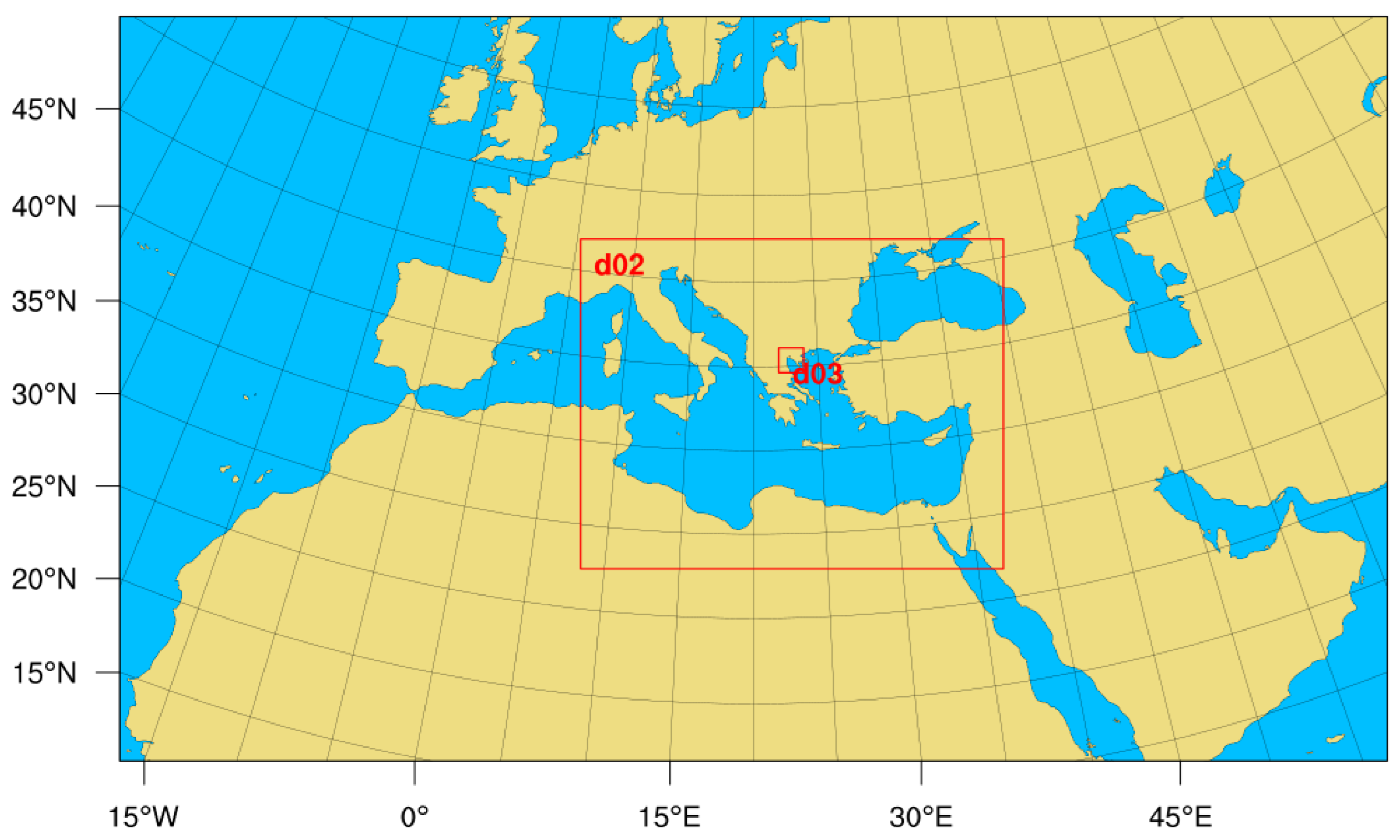
Climate simulations were conducted using the Weather Research and Forecast (WRF) meteorological model v4.1 [
16] for the representation of present and future climate in this study. Four telescoping domains for Europe, southeastern Mediterranean and Thessaloniki, with horizontal grid resolutions of 50 km (d01), 10 km (d02), and 2 km (d03), were utilized (
Figure 1). The configuration of the WRF vertical layers consisted of 35 unevenly spaced full sigma layers, extended up to 100 hPa. On the basis of previous evaluations of the WRF for the urban area of Thessaloniki [
17,
18], the physics schemes selected were (a) the Kain–Fritsch cumulus scheme (activated for domains d01 and d02) [
19], (b) the cloud microphysics WSM6 [
20], (c) the planetary boundary layer YSU [
21] coupled with the revised Monin–Obukhov surface layer parameterization of Jiménez et al. (2012) [
22], (d) the RRTMG for the short and long wave radiation [
23], (e) the Noah land model [
24], and (f) the single-layer urban canopy model (SLUCM) for the accurate representation of the urban fabric effects (e.g., street canyons) [
25].
The simulations were implemented for three 5 year periods, covering the present (2006–2010), the near future (2046–2050), and the distant future (2096–2100) climate, enabling the investigation of the buildings’ energy demand due to climate change by the end of the 21st century. The initial and boundary conditions, which were used to drive the regional setup of WRF, were the bias-corrected outputs of the NCAR Community Earth System Model version 1 (CESM1) [
26]. CESM1 participated in phase 5 of the Coupled Model Intercomparison Experiment (CMIP5). Moreover, the relative CMIP5 model performance for different atmospheric variables was calculated from the 1980–2005 climatological seasonal cycle of the CMIP5 historical simulations, revealing that CESM1 falls within the group of models with generally better performance than the median of all model results for many variables, with the most striking exception being the global average temperatures at 200 hPa, where most but not all models have a systematic bias. This comment of the reviewer is very useful, and a comparative analysis with the use of an ensemble of GCMs to drive the WRF regional application can be considered in future research. The output variables were corrected making use of the European Center for Medium-Range Weather Forecasts (ECMWF) Interim Reanalysis (ERA-Interim) fields for 1981–2005 [
27], which have been broadly used by numerous studies focusing on future climate projections [
28,
29,
30,
31]. The data were available for 26 pressure levels, at 6 h intervals with a spatial resolution of 1° under the Representative Concentration Pathway 8.5 (RCP8.5), the so-called “business-as-usual” climate scenario. Many studies have investigated the future climate under the RCP8.5 scenario, as it is the most aggressive and threatening scenario [
32,
33,
34,
35,
36,
37].
RCP8.5 was also selected for this study as the “worst-case” scenario for the estimation of the energy demand. Time series of temperature, relative humidity, pressure, wind speed and direction, and the accumulated fields of global horizontal irradiance, direct normal irradiance, and total short-wave diffuse radiation (sky + surface reflected) were extracted from the WRF outputs for the location of the building using the nearest-neighbor method at 3 h time intervals to be used as input of the energy consumption model. The WRF setup used in the present study was evaluated in Keppas et al. (2021) [
37], where satisfactory performance of the model in the area of Thessaloniki was shown. The 3 h data were imported to the simulation software. TRNSYS does not support a timestep higher than 1 h; thus, the imported 3 h data were automatically interpolated, and the simulation was run producing hourly results.
The most significant meteorological parameters, according to the WRF outputs and in connection to the initial boundary conditions selected, are presented in
Table 1. We can observe that the increase in temperature was significant, with the average temperature increasing by about 3.5 °C between the base scenario and the far future scenario. At the same time, a large increase in minimum temperature levels by approximately 8 °C is evident, with the minimum observed temperature for the period 2096–2100 reaching −2 °C. Humidity levels showed no significant changes and remained almost constant over the years.
2.2. Building Description
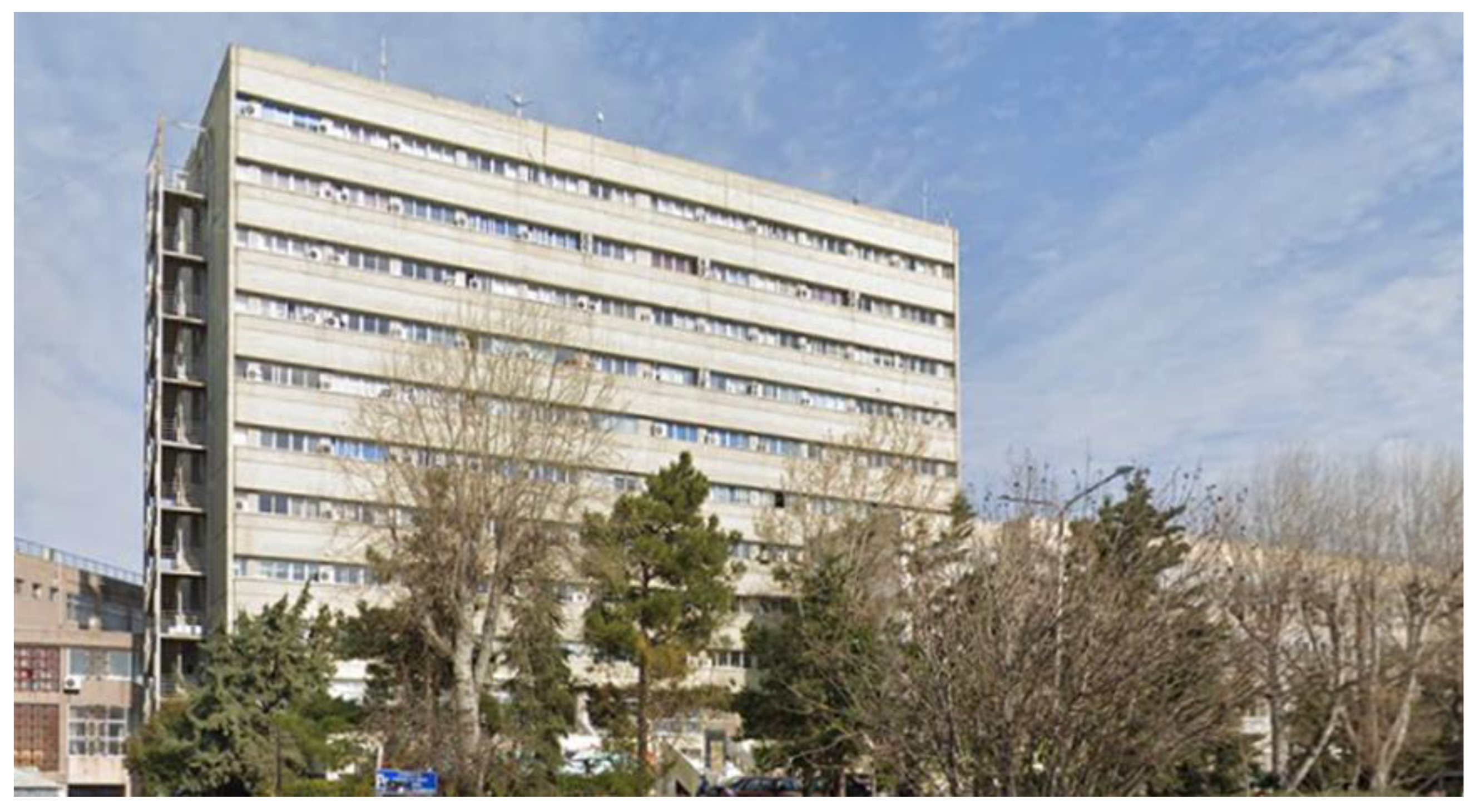
The building under study was Building D’ of the Faculty of Engineering of the Aristotle University of Thessaloniki, located between the Egnatia and 3rd September streets. Building D’ is a nine-story building that houses the offices of the faculty’s teaching and research staff, as well as some laboratories, which are mainly located in the basement, while the secretariats of the various departments are located on the ground floor of the building.
The building has a total volume of 44,671,197 m
3 and a total surface of 10,595,451 m
2, of which 29,017,462 m
3 and 8,167,691 m
2 correspond to heated spaces, respectively. The building is insulated according to the Greek national Thermal Insulation Regulation established in 1979 [
38], and it has not been renovated since its construction. The total actual external surface of the building shell (walls, glazing, roof, and floor), which is exposed to the outside air, for the building under study is A = 8714.90 m
2. The total area of glazing amounts to 1147.78 m
2.
2.3. Thermal Zones
The building under study was divided into 14 thermal zones to ensure a more precise energy analysis. These zones are presented in
Table 2.
On floors 1–9, 70% of the surface corresponds to offices, while the remaining 30% corresponds to corridors and ancillary spaces. Auxiliary spaces make up 70% of the zone corresponding to the building’s ground floor, while offices and secretariats make up 30%.
2.4. Operating Conditions
The thermal zones of the specific building belong to two types of uses. One is the use of the offices, and the other is that of the corridors and ancillary spaces. The technical guidelines issued by the Technical Chamber of Greece (T.O.T.E.E. 20701-1), the Regulation for the Energy Performance of Buildings (KENAK), and ASHRAE STANDARD 90.1 [
39] were used to choose the internal operation conditions of each thermal zone. The KENAK regulation was recently revised to comply with the Energy Performance of Buildings Directive (EPBD) [
40]. The selection was made with the aim of ensuring satisfactory levels of thermal comfort for all occupants [
41], and the resulting conditions are summarized in
Table 3. The cooling setpoint was chosen from the KENAK regulation, while the heating setpoint was selected from the ASHRAE STANDARD 90.1, because KENAK’s heating setpoint of 20 °C was deemed inadequate.
2.5. Building Shell and HVAC Systems
2.5.1. Building Shell
As mentioned in
Section 2.1, the building is thermally insulated according to the Regulation on Thermal Insulation of Buildings [
38]. The values of the total thermal permeability for each of the external structural elements were calculated and used as inputs in TRNSYS. The external walls consist of five layers of materials (internal and external plaster, two layers of bricks, and 3 cm expanded polystyrene core insulation). This results in a total coefficient of thermal transmittance equal to 0.71 W/m
2K. The roof consists of five layers of materials (internal coating, concrete, 3 cm expanded polystyrene insulation, waterproofing, and cement slabs), resulting in a total U-value coefficient equal to 0.77 W/m
2K. The floor in contact with the ground consists of three layers of materials (marble slabs, cement mortar, and concrete), resulting in a total heat transfer coefficient equal to 3.11 W/m
2K. The windows consist of double-glazed aluminum frames with a total U-value coefficient equal to 2.82 W/m
2K and a g-value coefficient equal to 0.64.
2.5.2. HVAC Systems
In the building, there is a central heating installation to meet the needs for heating. The installation includes two natural gas boilers with an efficiency rating of 90%, along with a high-temperature water distribution network and relatively insufficient piping insulation. The distribution network is 96% efficient and has a compensation system to deal with partial loads. In 2009, a monitoring and remote-control system (scada) was put into operation in the boiler room, achieving better management of the operation of the boilers and leading to reduced fuel consumption. The total rated power of boiler systems is 600 kW, according to the technical specifications of the manufacturer. The terminal heating units are classic AKAN-type water radiators with thermostatic heads mounted in each radiator and an efficiency of 89% [
41]. Local air-cooled heat pumps with a total power of 350 kW are used for cooling. The heat pumps are fairly outdated, and they do not have an energy label. An efficiency of COP = 2.5 was considered for these units on the basis of the date of construction according to KENAK, while the corresponding efficiency of the terminal units was equal to 93% [
41].
2.6. Building Modeling and Simulation
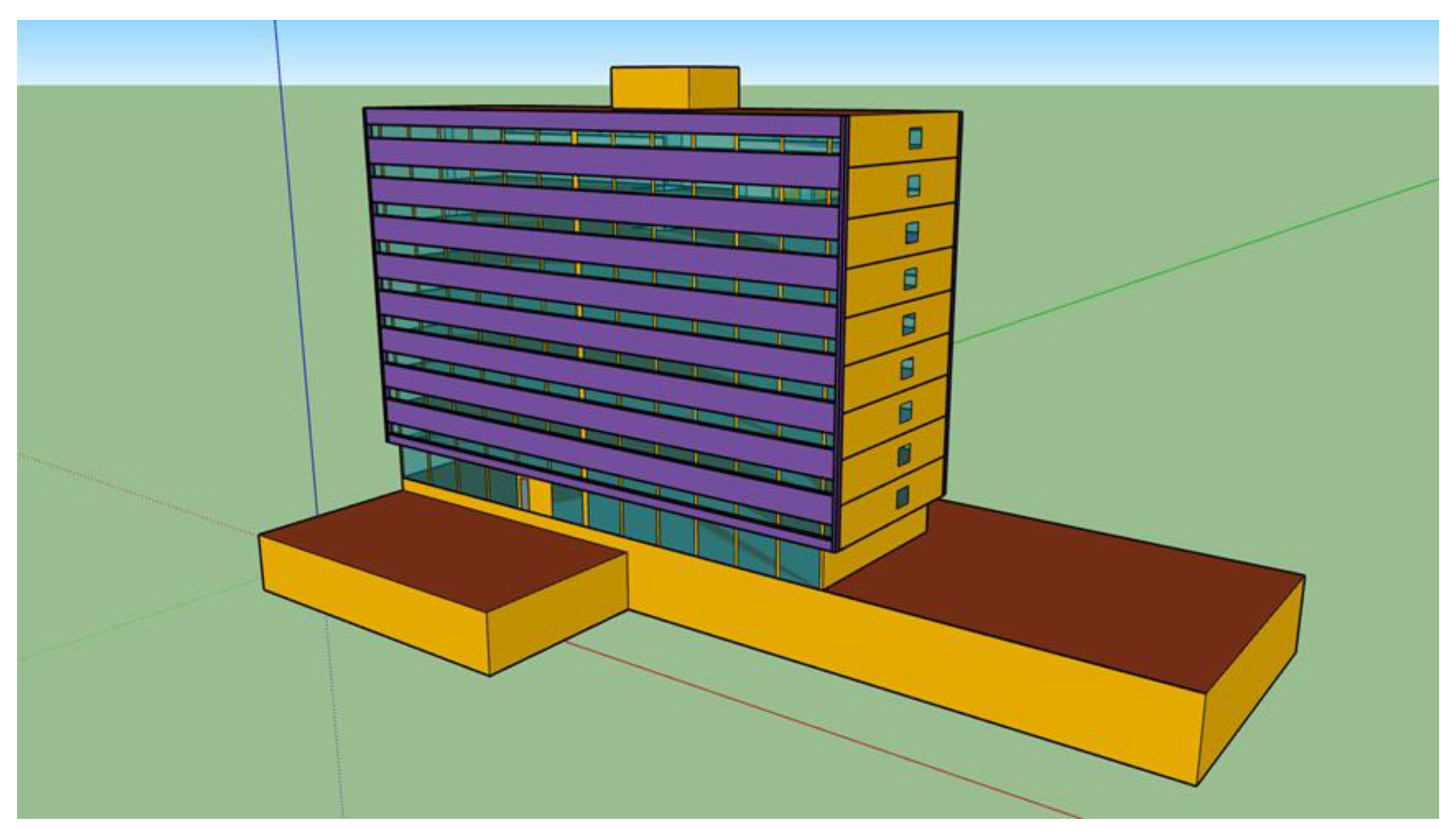
Two key components made up the simulation. After modeling the building geometry in the SketchUp software environment, energy modeling was carried out in TRNSYS [
42]. The model was created using information about the actual building’s measurements, architectural features, orientation, and shadings (
Figure 2 and
Figure 3). Following the building model’s import into TRNSYS, all structural parameters including walls, windows, doors, the schedules for occupancy, lighting, and appliances, the internal loads, and the HVAC system operation schedules and setpoints were defined. The building model was completed by adding the necessary climatic data using the custom weather files (temperature, relative humidity, radiation, etc.).
3. Results and Discussion
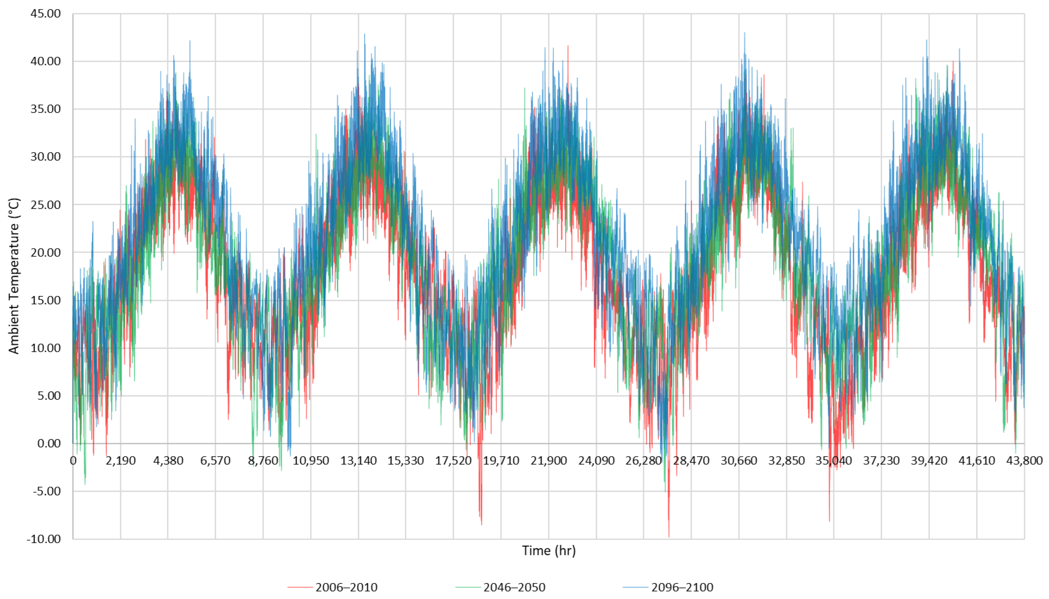
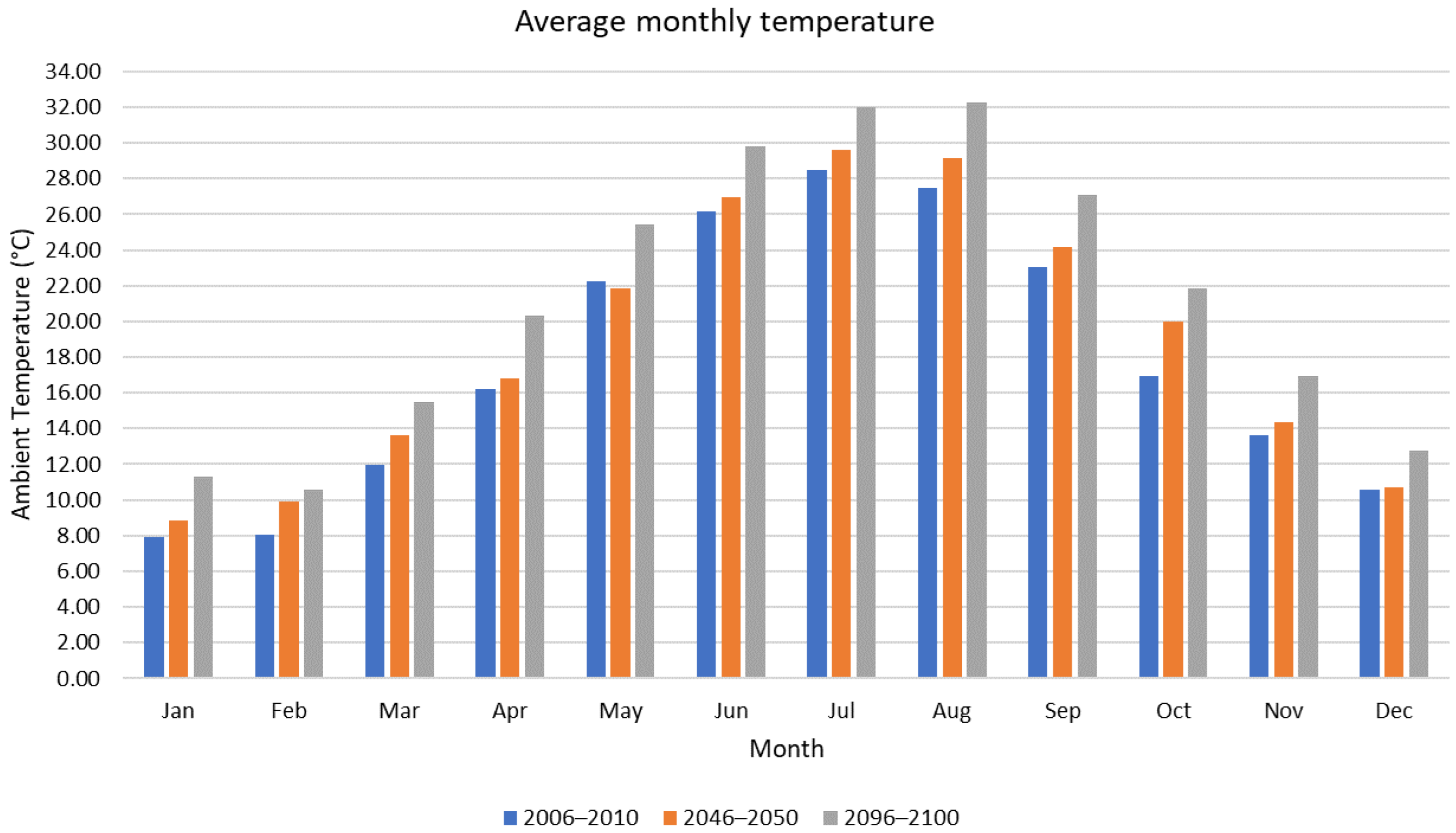
The results of the simulation are presented in this section. Hourly ambient temperature is depicted in
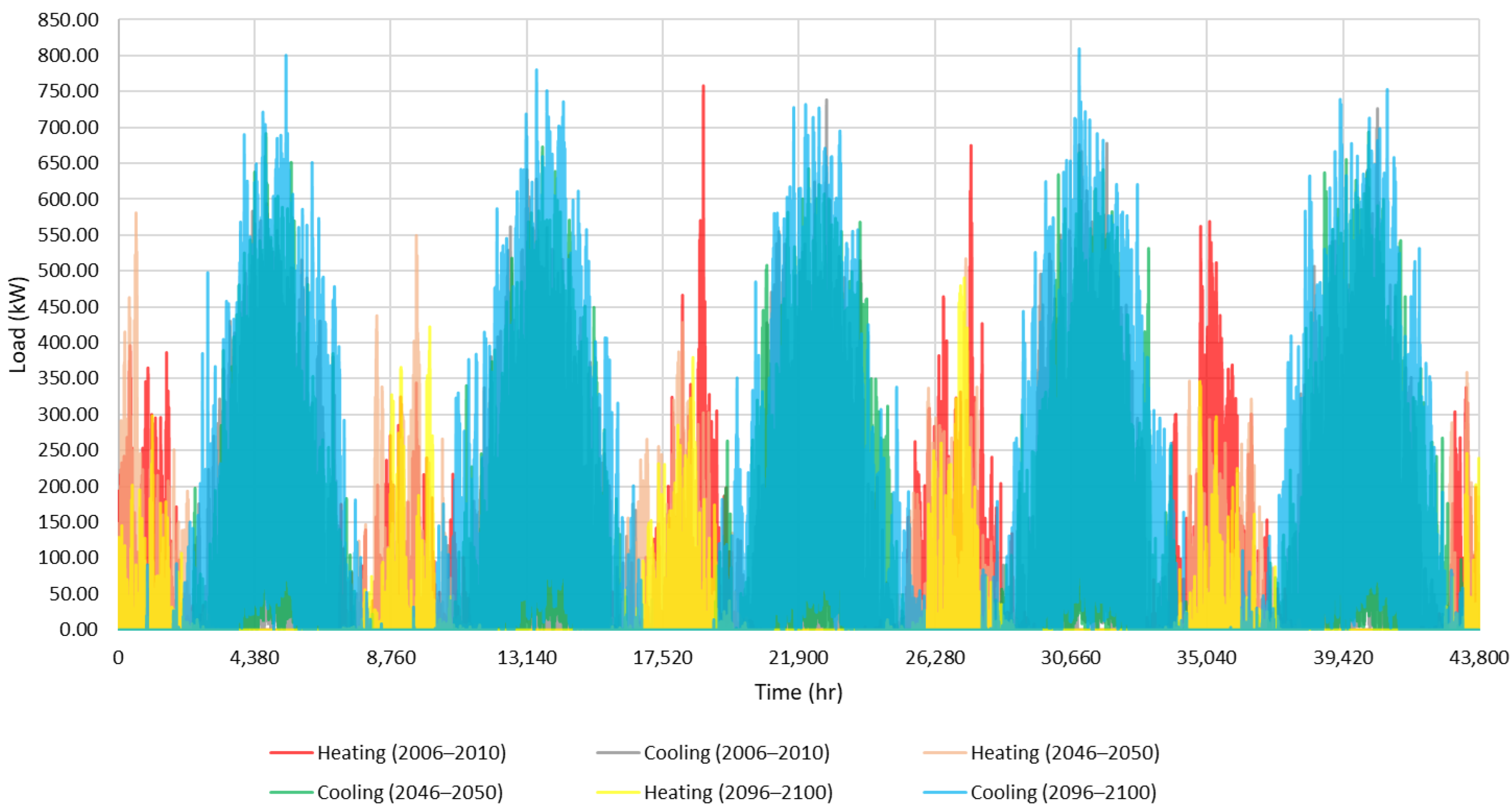
Figure 4. Hourly energy demand for heating and cooling (sensible and latent) is illustrated in
Figure 5. Furthermore, the monthly energy demand is presented in
Figure 6. The temperature increase was evident during each year. It was particularly evident during the summer months with the temperature in several cases exceeding 35 °C during the 5 year period 2046–2050 and 40 °C during the 5 year period 2096–2100. The temperature in the winter period remained almost at the same level for every dataset, with recorded minimum temperatures not exceeding −10 °C.
It is noticeable that there was a continuous upward trend in terms of ambient temperature dependent on the RCP8.5 forcing scenario selected. The increase in temperature led to a change in the energy balance of the building, but only a slight increase in the total energy consumption. This is due to the fact that the cooling loads were covered by heat pumps whose seasonal energy efficiency SCOP = 2.5. Therefore, it can be concluded that the effects of the increase in cooling loads had a relatively small impact on the energy consumption of the building. However, the consumption comparison was made considering a constant COP that does not depend on the ambient temperature. Taking into account that the energy efficiency is reduced when the heat pumps operate in cooling mood while the outdoor temperature is increased, the energy consumption in that case would also increase. In addition, the increase in peak loads for cooling was evident from the diagrams. Such an increase in loads led to inadequacy of the existing system to meet the loads.
The simulations were implemented for 5 year periods in order to extract manageable and comparable results. The mean monthly energy consumption requirements for heating and cooling for each 5 year period are presented in
Figure 7 (specific energy consumption per surface area, kWh/m
2).
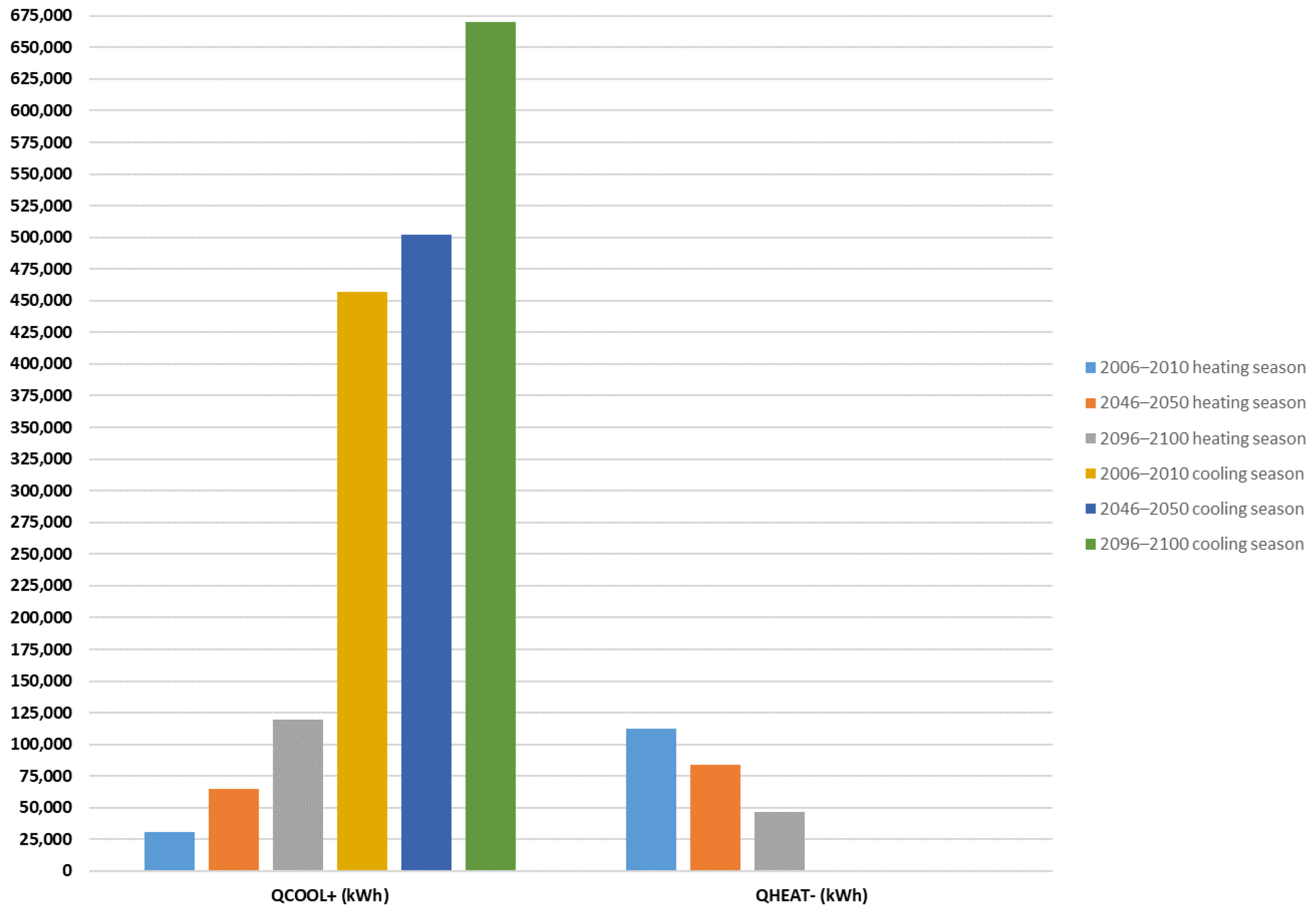
Figure 7 displays the mean annual energy needs for heating and cooling in absolute terms (kWh/year). On the basis of the predicted and meteorological data, it is shown that cooling loads significantly increased, leading to higher energy requirements for cooling than for heating. The most significant energy requirements to satisfy the cooling loads were noted for the 5 year periods 2046–2050 and 2096–2100.
The increase in cooling loads was particularly strong, with cooling loads increasing by 16% for the period 2046–2050 and by 62% for the period 2096–2100 (
Table 4). There was a slight decrease in heating loads for each 5 year period, but the increase of cooling loads still outperformed the decreased heating loads, leading to an increase in total loads (heating and cooling). Total loads increased by 9% during 2046–2050 and by 39% during 2096–2100. Despite the increase in total loads, the energy consumption of the building remained at the same level as the baseline for the 2046–2050 period and increased by only 5% during 2096–2100 (
Table 5).
Figure 7 highlights the substantial rise in cooling loads in particular. The outcomes during both the heating and the cooling season are depicted in the diagram. We can see that the cooling loads significantly outweighed the heating loads, which were nearly nonexistent, for the 5 year period 2096–2100. In
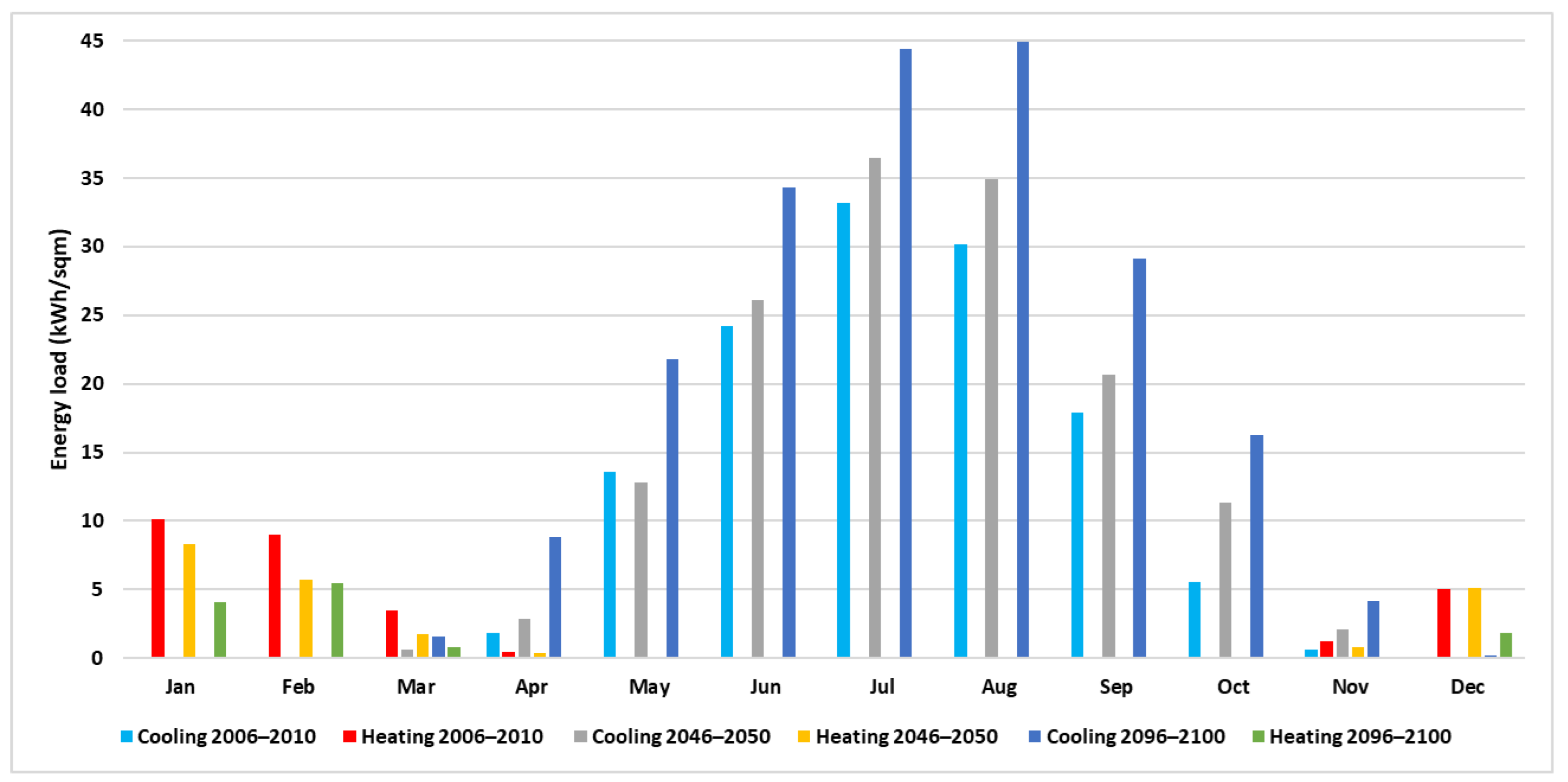
Figure 8, the monthly loads for heating and cooling for each period under study are presented. It is evident that, during the pure winter months, i.e., the months of December, January, and February, there was a slight decrease in heating loads over the years, while the cooling loads remained constant. During the summer months, i.e., May, June, July, August, and September, a steady increase in cooling loads could be observed over the years. The effect of future data on the energy balance of the transition period was impressive, where it was observed that, from an initially almost balanced situation between cooling and heating, we moved to a situation where cooling loads clearly prevailed. To sum up, the best hope for the building sector’s decarbonization over the next few decades will be a reduction in cooling loads and an evolution of air-conditioning systems, always in conjunction with a more general European energy and environmental strategy. In addition, the utilization of the energy flexibility of buildings and their HVAC systems will hopefully enhance the ability of buildings and their users to survive under climate change and extreme climate events [
43].
The prediction of the energy loads can highlight the processes where interventions should be made in order to achieve energy efficiency and reduced carbon emissions. The added value of the holistic design and evaluation of buildings is that, in addition to the technical efficiency with regard to central heating and air-conditioning systems for buildings, other goals can be accomplished such as thermal comfort and indoor air quality, which result from the dynamic simulation focusing on HVAC system operation, indoor environmental parameters (air flow, air infiltration, and thermal comfort), and occupants’ behavioral characteristics. The abovementioned parameters can be used in order to ensure energy-efficient buildings, as well as improve the quality for living. Technology can ensure an upgrade of building energy systems by implementing, e.g., smart metering for monitoring thermal comfort and air quality, thus providing easier-to-use portable tools for gathering highly temporally resolved data in real time. Future analyses will focus on the evaluation of ventilation systems in collaboration with other energy systems and innovative technologies providing the health and wellbeing of occupants, along with resilience in the building’s management [
44].
4. Conclusions and Future Research
It is essential, according to the European policy for energy and the environment, to design, construct, and manage the built environment in a more sustainable and resilient manner. Climate change is a global challenge which significantly affects urban life and nature. The extreme weather events and the rise of in temperatures impact the environment in several ways. Mitigation and adaptation measures should be taken in order to react efficiently in the climate change issue. The carbon neutrality vision for buildings is an issue of integrated management which mainly focuses on the most energy-intensive processes such as heating and cooling.
When calculating the energy loads, the input data represent a critical parameter for the quality of the output results. However, it is of great importance whether standard weather data are reliable and adequate to define the current situation and to assist in designing buildings that behave efficiently with regard to climate conditions. To achieve the goal of designing climate-proof buildings, the Weather Research and Forecast meteorological model (WRF) was used to predict future climate scenarios. There are several approaches for creating meteorological datasets that can be used in building energy simulation. In this study, we used downscaling to create data for the near and far future. Past data were used to ensure the model’s database efficiency; then, considering RCA4 and RCP8.5, the data were downscaled, and future meteorological data of periods 2046–2050 and 2096–2100 were created. It was discovered during the investigation that the effects of climate change varied depending on the case studies. Therefore, it is crucial to apply a regional and localized analysis when developing future meteorological data.
The outcomes also showed that the downscaling approach may deliver sufficient data to enable a comparison analysis of long-term improvements in energy building performance. It is advised that further research can be conducted with regard to model uncertainties of RCMs by taking into account the use of an ensemble-based methodology. Additionally, it is crucial to keep in mind that RCMs have been used for both historical and future time periods. In order to decrease uncertainties and improve physical consistency, these models may be compared to real data, and the biases associated with the climate model data can be modified.
The results presented that, for the future weather data, there was a significant effect on the energy balance of the building. This effect was mainly focused on the increase of the cooling loads in the building, as well as on the reduction in the observed heating loads to a certain extent. Total consumption was affected, and a 5% increase was finally observed in the 2096–2100 scenario compared to the reference scenario. According to the climate data and the observed loads of the building, the winter months in which heating loads were observed were mainly limited to three (December, January, and February). This highlights the importance of reviewing the way in which buildings are designed. Today’s buildings in the area of Thessaloniki were built with the aim of reducing both thermal and cooling loads. On the basis of the results of this research, special emphasis must be given to the reduction in cooling loads in future constructions. This is the benefit of estimating the energy loads, as well as the consumption during the decision-making process, whereby interested parties can prioritize the interventions considering the upgrade of buildings in relation to energy performance. Therefore, interventions that mainly concern the frames, the insulation of the roof, and the use of innovative air-conditioning systems should be implemented. These interventions are effective because they are focused on reducing the energy loads, which will be increased in the future according to the predictive weather data. Therefore, by controlling the energy loads, the energy consumption can also be monitored. The effect of future data on the energy balance of the transition period is impressive, where it was observed that, from an initially almost balanced situation between cooling and heating, we are moving to a situation where cooling loads clearly prevail. To sum up, on the basis of the simulation results, along with the vision of decarbonization and energy resilience in the building stock, the weather changes will affect the energy consumption. More specifically, in the next few decades, there will be a reduction in cooling loads, and air-conditioning system technology should be upgraded in conjunction with a more defined European energy and environmental strategy. Without doubt, the building sector represents a challenging task. As part of further research, other building typologies not limited to Greece and Mediterranean countries will be studied. Typical constructions on existing buildings will be studied in other EU countries in order to provide more detailed recommendations while taking into consideration different climatic conditions.


 ,
, 


