Settling of Mesoplastics in an Open-Channel Flow

Abstract

Pollution of water by plastic contaminants has received increasing attention, owing to its negative effects on ecosystems. Small plastic particles propagate in water and can travel long distances from the source of pollution. In order to research the settling motion of particles in water flow, a small-scale experiment was conducted, whereby spherical plastic particles of varying diameters were released in an open-channel flow. Three approaches were investigated to numerically simulate the motion of particles. The numerical simulation results were compared and validated with experimental data. The presented methods allow for deeper insight into particle motion in fluid flow and could be extended to a larger scale to predict the propagation of mesoplastics in natural environments.

1. Introduction

Research on the topic of particle motion is ongoing. Many pollutants that are present in the environment form a dispersed multiphase system, in which the continuous phase is the medium of the environment (gas or liquid) and the dispersed phase is made of pollutant particles. Plastic particles with diameters between 1 and 10 mm, termed mesoplastic particles or mesoplastics, represent a ubiquitous and concerning pollutant [1,2]. However, there is still a lack of consensus with respect to the definition of plastic debris size classification [1,2,3]. In the literature, plastic particles with diameters of less than 5 mm are often classified as microplastic particles or microplastics [3,4,5].

One source of pollution is the wastewater generated by various industries [6], for example, the textile industry [7]. Owing to the negative impact of plastic particles on the environment, it is of particular interest and importance to research how they spread in the environment [8,9,10,11,12,13]. The propagation of mesoplastics occurs in rivers and oceans; therefore, the topic of the motion of particles suspended in water should be the focus of further research [14,15]. Depending on their properties, mesoplastics can settle and propagate as sediment, flow freely suspended with water or float on the free surface of the water. In rivers, natural and man-made obstacles exist, which produce different flow features and regimes that can be replicated in a laboratory-scale physical model to investigate various scientific and engineering problems with respect to different modes of mesoplastic propagation.

The transport of particles on a laboratory scale has been studied in open-channel flows in the past. Cook et al. [16] experimentally studied the longitudinal dispersion of microplastic particles and suggested the use of a fluorescent tracer to study the movement of plastic particles in the environment. Yu et al. proposed an empirical formula to predict the incipient motion of microplastic particles with diameters up to 5 mm [17]. The general importance and applicability of studying particle settling was highlighted in an article by Yi and colleagues, who studied the settling of sturgeon eggs in an open channel [18]. In addition to experimental work, different numerical simulation approaches have been used to study the propagation of plastic particles. The dispersal of microplastic particles in coastal waters was studied by Fatahi and colleagues [15] using computational fluid dynamics (CFD); a discrete phase model (DPM) was used to track the motion of particles. Roy et al. [19] conducted a parametric study of plastic particle propagation using a Lagrangian tracking model in a lid-driven cavity flow. On a larger scale, an Eulerian modelling approach is sometimes adopted, as in a study of the transport and deposition of microplastic particles in the Baltic sea conducted by Schernewski et al. [14], who concluded that microplastic emissions resulted mostly from wastewater, as well as sewer and stormwater overflow. Another approach to Lagrangian tracking is the dense discrete phase model (DDPM), which is often used to simulate particle-laden flows in pipelines [20]. Recent attempts to model the motion of microplastic or mesoplastic particles include works by Holjević et al. [21] and Travaš et al. [22], who modelled the transport of different microplastic (or mesoplastic) particles in a laminar open-channel flow.

In this work, the settling of mesoplastic particles is investigated in a 3D turbulent open-channel flow using numerical simulations and experiments.

2. Materials and Methods

Two methods of Lagrangian tracking of particles in fluid flow, available as part of ANSYS Fluent, a commercial computational fluid dynamics (CFD) software, were used in this work. The first is the discrete phase model (DPM) [23], in which the particles are assumed to be point masses, and their volume is not accounted for in the equations of fluid flow. The second is the dense discrete phase model (DDPM) [23], in which the volume of particles are accounted for in the governing equations of fluid flow via their volume fraction. Within the DDPM framework, particle–particle interaction can be included. Multiple approaches are available to describe particle–particle interaction; in this work, this interaction is investigated via the discrete element method (DEM). To this end, an additional DEM software is used, Altair EDEM, and connected to ANSYS Fluent to exchange information about particles.

2.1. Discrete Phase Model

2.1.1. Liquid Flow

The governing equations of flow are continuity Equation (1) and the Navier–Stokes Equation (2)

$$\frac{\partial \left({\rho }_c\right)}{\partial t}+\nabla ·\left({\rho }_c\mathit{u}\right)=0,$$

(1)

$$\frac{\partial \left({\rho }_c\mathit{u}\right)}{\partial t}+\nabla ·\left({\rho }_c\mathit{u}\mathit{u}\right)=-\nabla p+{\mu }_c{\nabla }^2\mathit{u}+{\rho }_c\mathit{g}+{\mathit{S}}_M,$$

(2)

where ${\rho }_c$ is the continuous phase (liquid) density, $\mathit{u}$ is the continuous phase (liquid) velocity, ${\mu }_c$ is the continuous phase (liquid) dynamic viscosity and $p$ is the pressure in the continuous phase (liquid). The term ${\rho }_c\mathit{g}$ represents the gravitational force, where $\mathit{g}$ is the gravitational acceleration.

The presence of particles in the flow can affect the flow field, which is accounted for by the additional momentum term ${\mathit{S}}_M$. For turbulence, the RANS approach is adopted with the realizable k − ε turbulence model, where two additional transport equations for turbulence kinetic energy (k) and dissipation of turbulence kinetic energy (ε) are used.

$$\frac{\partial \left({\rho }_{c}k\right)}{\partial t}+\nabla ·\left({\rho }_{c}k\mathit{u}\right)=\nabla ·\left[\left({\mu }_c+\frac{{\mu }_t}{{\sigma }_k}\right)\nabla k\right]+G_k+G_b-{\rho }_c\epsilon -Y_M+S_k,$$

(3)

$$\frac{\partial \left({\rho }_c\epsilon \right)}{\partial t}+\nabla ·\left({\rho }_c\epsilon \mathit{u}\right)=\nabla ·\left[\left({\mu }_c+\frac{{\mu }_t}{{\sigma }_{\epsilon }}\right)\nabla \epsilon \right]+{\rho }_c{C}_{1}S\epsilon -{\rho }_c{C}_2\frac{{\epsilon }^2}{k+\sqrt{\nu \epsilon }}+C_{1\epsilon }\frac{\epsilon }{k}{C}_{3\epsilon }{G}_b+S_{\epsilon },$$

(4)

where the coefficients are

$$C_1=max\left[0.43;\frac{\eta }{\eta +5}\right],$$

(5)

$$\eta =S\frac{k}{\epsilon },$$

(6)

and the strain rate magnitude is

$$S=\sqrt{2\mathit{S}\mathit{S}}.$$

(7)

The model constants are $C_{1\epsilon }=1.44$, $C_2=1.9$, ${\sigma }_k=1.0$ and ${\sigma }_{\epsilon }=1.2$. The expression for eddy viscosity (${\mu }_t$) is

$${\mu }_t={\rho }_c{C}_{\mu }\frac{k^2}{\epsilon }$$

(8)

In contrast to the standard k − ε model, the coefficient ($C_{\mu }$) is a function of mean strain, mean rotation rate, turbulence kinetic energy and dissipation of turbulence kinetic energy. In Equations (3) and (4), there are additional terms that describe the production of turbulence kinetic energy ($G_k$), buoyancy effects ($G_b$) and compressibility effects ($Y_M$). ${\sigma }_k$ and ${\sigma }_{\epsilon }$ are the turbulent Prandtl numbers for the turbulent kinetic energy (k) and the dissipation of turbulent kinetic energy (ε), respectively. To account for the effects of particles on turbulence, source terms for the turbulence kinetic energy ($S_k$) and the dissipation of turbulence kinetic energy ($S_{\epsilon }$) are also included.

2.1.2. Particle Motion

Particles are tracked in the Lagrangian frame; particle position and velocity are obtained by integration of the governing ordinary differential equations along the particle trajectory. The motion of a single particle is governed by the conservation of mass equation and Newton’s second law.

$$\frac{d{m}_p}{dt}=0,$$

(9)

$$m_p\frac{d\mathit{v}}{dt}=\mathit{F},$$

(10)

$$I_p\frac{d\mathsf{\omega }}{dt}=\mathit{M},$$

(11)

where $m_p$ is the particle mass, $I_p$ is the particle moment of inertia, $\mathit{v}$ is the particle velocity, $\mathit{\omega }$ is the particle angular velocity, $\mathit{F}$ is the resultant force on the particle and $\mathit{M}$ is the resultant torque on the particle. The forces acting on the particle are the drag (${\mathit{F}}_{\mathit{d}}$), the buoyancy force (${\mathit{F}}_{\mathit{b}}$), the gravitational force (${\mathit{F}}_{\mathit{g}}$), the pressure gradient force (${\mathit{F}}_{\mathit{p}\mathit{g}}$), the virtual mass force (${\mathit{F}}_{\mathit{v}\mathit{m}}$) and the Magnus lift due to particle rotation (${\mathit{F}}_{\mathit{m}\mathit{l}}$):

$$m_p\frac{d\mathit{v}}{dt}={\mathit{F}}_{\mathit{d}}+{\mathit{F}}_{\mathit{b}}+{\mathit{F}}_{\mathit{g}}+{\mathit{F}}_{\mathit{p}\mathit{g}}+{\mathit{F}}_{\mathit{v}\mathit{m}}+{\mathit{F}}_{\mathit{m}\mathit{l}},$$

(12)

These forces are expressed as:

$${\mathit{F}}_{\mathit{d}}=m_p\frac{18{\mu }_c}{{\rho }_p{d}_p^2}\frac{C_{D}R{e}_p}{24}\left(\mathit{u}-\mathit{v}\right),$$

(13)

$${\mathit{F}}_{\mathit{b}}+{\mathit{F}}_{\mathit{g}}=m_p\frac{\mathit{g}\left({\rho }_p-{\rho }_c\right)}{{\rho }_p},$$

(14)

$${\mathit{F}}_{\mathit{p}\mathit{g}}=m_p\frac{{\rho }_c}{{\rho }_p}\frac{D\mathit{u}}{Dt},$$

(15)

$${\mathit{F}}_{\mathit{v}\mathit{m}}=\frac{1}{2}{m}_p\frac{{\rho }_c}{{\rho }_p}\left(\frac{D\mathit{u}}{Dt}-\frac{d\mathit{v}}{dt}\right),$$

(16)

$${\mathit{F}}_{\mathit{m}\mathit{l}}=\frac{1}{2}{A}_p{C}_{RL}{\rho }_c\frac{\left|\mathit{u}-\mathit{v}\right|}{\left|\Omega \right|}\left(\left(\mathit{u}-\mathit{v}\right)\times \Omega \right),$$

(17)

where ${\rho }_p$ is the particle density, $d_p$ is the particle diameter, $C_D$ is the drag coefficient, $R{e}_p$ is the particle Reynolds number, $A_{\mathit{p}}$ is the projected particle surface area, $C_{RL}$ is the rotational lift coefficient and $\Omega$ is the relative angular velocity of the particle. For the drag coefficient ($C_D$), a correlation by Morsi and Alexander [24] is adopted, as it is applicable over a wide range of Reynolds numbers.

For the rotational lift coefficient ($C_{RL}$), an approach proposed by Tsuji et al. [25] is adopted, as it is applicable to high particle Reynolds numbers (Re_p < 1600). The torque applied to the particle ($\mathit{M}$) can be expressed in terms of rotational drag acting on the particle. Equation (11) is rewritten as

$$I_p\frac{d\mathit{\omega }}{dt}=\frac{{\rho }_c}{2}{\left(\frac{d_p}{2}\right)}^5{C}_{\omega }\left|\Omega \right|·\Omega ,$$

(18)

where $C_{\omega }$ is the rotational drag coefficient. The correlation proposed by Dennis et al. [26] is used.

2.2. Dense Discrete Phase Model

2.2.1. Liquid Flow

The governing equations of flow presented in Section 2.1.1 are modified to account for the presence of the particles via their volume fraction

$$\frac{\partial \left({\alpha }_c{\rho }_c\right)}{\partial t}+\nabla ·\left({\alpha }_c{\rho }_c\mathit{u}\right)=0,$$

(19)

$$\frac{\partial \left({\alpha }_c{\rho }_c\mathit{u}\right)}{\partial t}+\nabla ·\left({\alpha }_c{\rho }_c\mathit{u}\mathit{u}\right)=-{\alpha }_c\nabla p+\nabla ·\left[{\alpha }_c{\mu }_c\left(\nabla \mathit{u}+{\mathit{u}}^T\right)\right]+{\alpha }_c{\rho }_c\mathit{g}+K_M\left(\mathit{v}-\mathit{u}\right)+{\mathit{S}}_{M,explicit},$$

(20)

where ${\alpha }_c$ is the continuous-phase volume fraction, $K_M$ is the particle-averaged interphase momentum exchange coefficient (implicit part of the momentum exchange with discrete phase) and ${\mathit{S}}_{M,explicit}$ is the momentum source term resulting from the displacement of fluid in the presence of a discrete phase.

2.2.2. Particle Motion

The governing equations of particle motion are the same as those described in Section 2.1.2. Equation (12) can be extended to include particle–particle interaction force (${\mathit{F}}_{\mathit{D}\mathit{E}\mathit{M}}$)

$$m_p\frac{d\mathit{v}}{dt}={\mathit{F}}_{\mathit{d}}+{\mathit{F}}_{\mathit{b}}+{\mathit{F}}_{\mathit{g}}+{\mathit{F}}_{\mathit{p}\mathit{g}}+{\mathit{F}}_{\mathit{v}\mathit{m}}+{\mathit{F}}_{\mathit{m}\mathit{l}}+{\mathit{F}}_{\mathit{D}\mathit{E}\mathit{M}}.$$

(21)

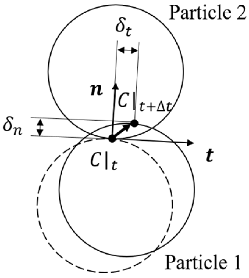
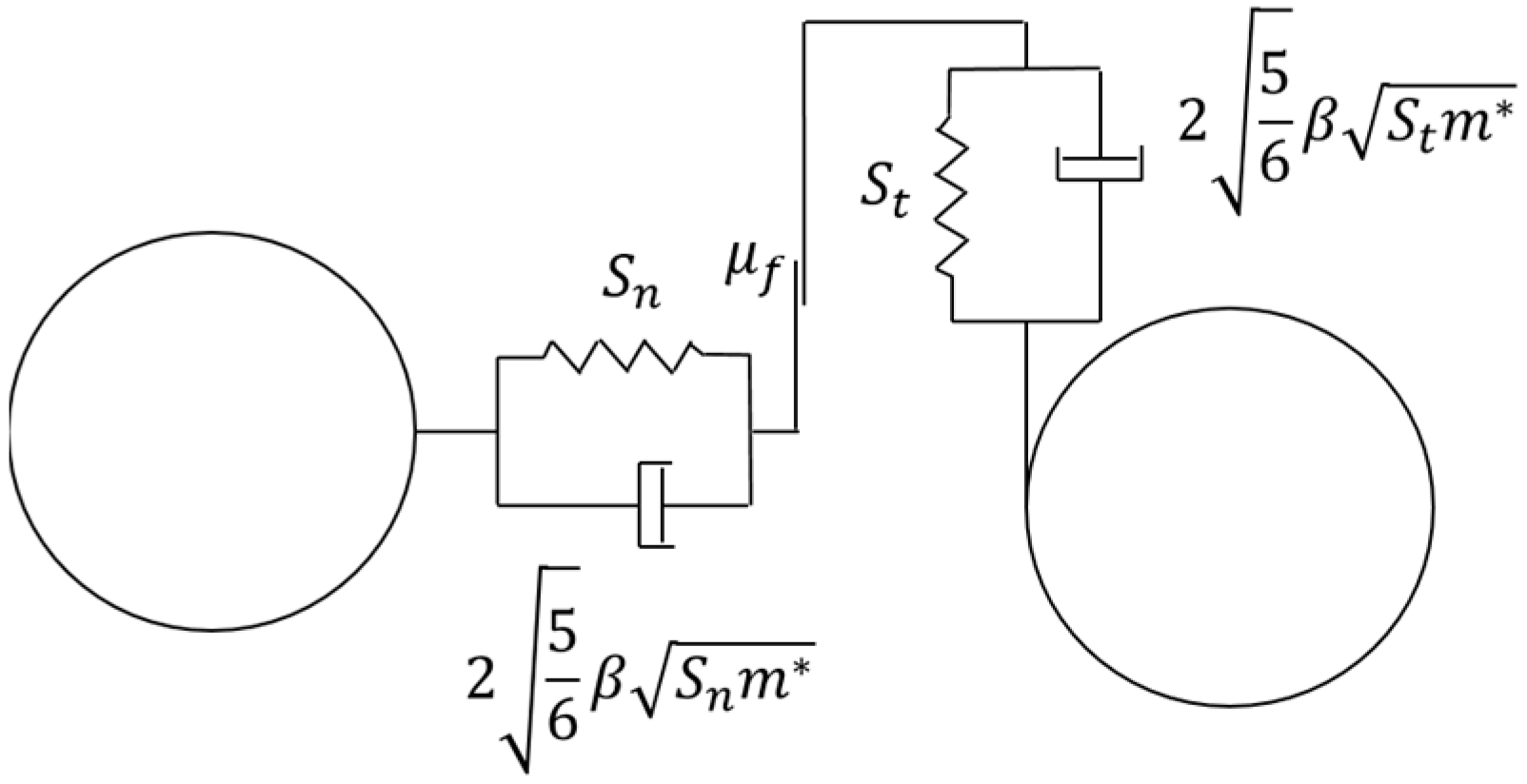
Particle–particle interaction is modelled according to DEM. Deformations of particles during collisions are accounted for by introducing the collision overlap between particles instead of collision deformations, as shown in Figure 1. Contact between colliding particles is modelled with the Hertz–Mindlin model [27,28], whereby the particle interaction is represented by a spring–dashpot system, as shown in Figure 2.

The particle interaction force is split into the normal and tangential components, where normal is defined at the point of contact between particles.

$${\mathit{F}}_{\mathit{D}\mathit{E}\mathit{M}}=F_{DEM,n}\mathit{n}+F_{DEM,t}\mathit{t}.$$

(22)

The normal and tangential components of the interaction force are expressed in terms of the spring–dashpot system as the spring force and the damping force.

$$F_{DEM,n}=F_{n, spring}+F_{n,damping}=\frac{4}{3}E*\sqrt{R*}{\delta }_n^{\frac{3}{2}}-2\sqrt{\frac{5}{6}}\beta \sqrt{S_{n}m*}{v}_{rel, n},$$

(23)

$$F_{DEM,t}=F_{t, spring}+F_{t,damping}=8G*\sqrt{R*{\delta }_n}{\delta }_t-2\sqrt{\frac{5}{6}}\beta \sqrt{S_{t}m*}{v}_{rel, t},$$

(24)

where $E*$ is the equivalent Young’s modulus, $G*$ is the equivalent shear modulus, $R*$ is the equivalent radius, ${\delta }_n$ is the overlap in the normal direction, ${\delta }_t$ is the overlap in the tangential direction, $\beta$ is a constant, $S_n$ is the normal stiffness, $S_t$ is the tangential stiffness, $m*$ is the equivalent mass, $v_{rel, n}$ is the normal component of the relative velocity and $v_{rel, t}$ is the tangential component of the relative velocity. These are defined as

$$\frac{1}{E*}=\frac{1-{\nu }_1^2}{E_1}+\frac{1-{\nu }_2^2}{E_2},$$

(25)

$$\frac{1}{G*}=\frac{2\left(1+{\nu }_1\right)\left(1-{\nu }_1^2\right)}{E_1}+\frac{2\left(1+{\nu }_2\right)\left(1-{\nu }_2^2\right)}{E_2},$$

(26)

$$\frac{1}{R*}=\frac{R_1+R_2}{R_1{R}_2},$$

(27)

$$\mathsf{\beta }=\frac{-\ln e}{\sqrt{{\ln }^{2}e+{\pi }^2}},$$

(28)

$$S_n=2E*\sqrt{R*{\delta }_n},$$

(29)

$$S_t=8G*\sqrt{R*{\delta }_n},$$

(30)

$$m*=\frac{m_1{m}_2}{m_1+m_2},$$

(31)

$$v_{rel, n}=v_{1, n}+v_{2, n},$$

(32)

$$v_{rel, t}=v_{1, t}+v_{2, t},$$

(33)

where $\nu$ is the Poisson ratio, E is the Young’s modulus, R is the particle radius, e is the coefficient of restitution, m is the particle mass, $v_n$ is the particle normal velocity and $v_t$ is the particle tangential velocity. Subscripts 1 and 2 refer to particle 1 and particle 2, respectively, in collision, as shown in Figure 1. Normal and tangential velocities of particles are observed according to the local collision coordinate system, as shown in Figure 1.

2.3. Experiment

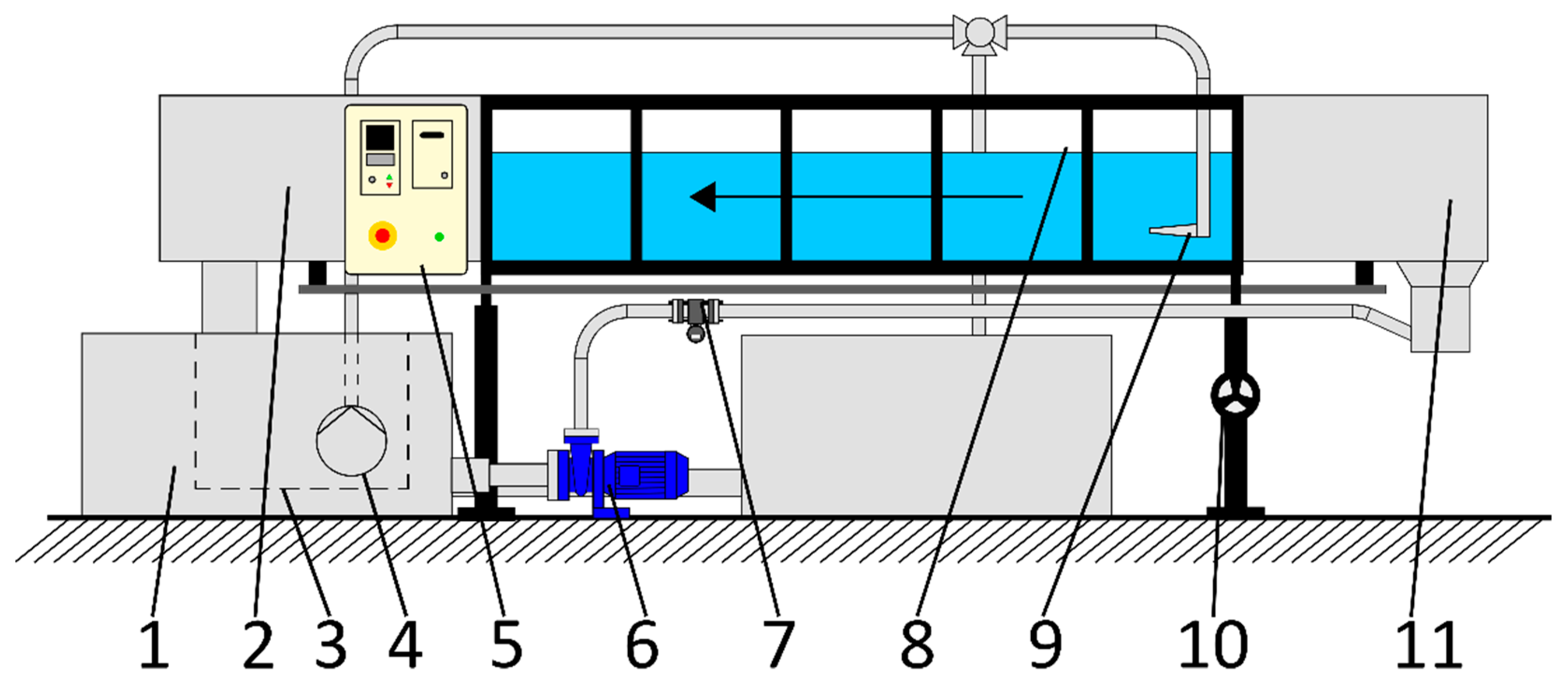
The Faculty of Civil Engineering of the University of Rijeka is home to the GUNT HM 162 experimental flume (shown on Figure 3), which is an open-channel flow physical model with a test section with a length of 12,500 mm and a rectangular cross section measuring 309 mm in width and 450 mm in height. This experimental flume is also fitted with a separate particle inlet.

The HM 162 experimental flume consists of an open-channel test section that is a part of a closed water circuit. The water is circulated from a water tank into the pipe and through the water inlet element into the experimental section by a Lowara SHS4 centrifugal pump, which can provide a maximum head of 16.1 m and has an operating flow rate in the range of 5.4 to 130 m³ h⁻¹. The water flows back into the water tank through the outlet element at the end of the experimental section. The water pump is controlled by the PLC (switch box) to adjust the flow rate. The actual flow rate is reported by the Endress+Hauser Promag 10L electromagnetic flow rate sensor, which is built into the pipe between the water pump and inlet section and has a measuring range of 5.4 to 180 m³ h⁻¹. The water level and the tilt of the open-channel section are also adjustable via the adjustable overflow edge and the inclination adjustment element, respectively.

The particle inlet that is supplied by GUNT (as shown in Figure 3) is intended for dense sediment flows, with high sediment flow rates achieved by means of a separate GUNT-manufactured sediment pump. The pump is designed for fine-grained sand with a granulation of up to 2 mm and can achieve a maximum flow rate of 36 m³ h⁻¹. Because this work is focused on small batches of particles that are passively introduced into the water and are larger than 2 mm, a new particle inlet was constructed at the hydraulic laboratory of the Faculty of Civil Engineering, University of Rijeka.

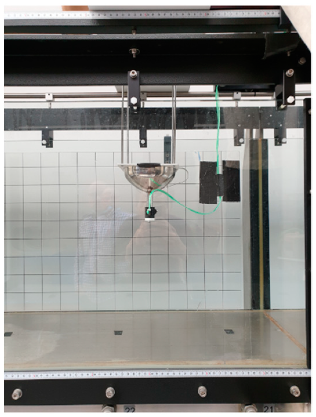
A metal funnel was fitted with a 3D-printed opening mechanism and fixed inside a 3D-printed holding plate. The holding plate was attached to four steel wires, which were attached to the base plate. When the base plate was placed on top of the experimental section side walls, the funnel was positioned as shown in Figure 4.

We investigated the settling and particle size distribution of 3D-printed spherical plastic particles with a density of 1140 kg m⁻³. The particle size distribution is presented in

Table 1. Particle sizes used in the settling experiment.

Particle Diameter (mm)	2	2.5	3.5	4
Number of particles	62	67	70	58
Color	Black	Red	Green	White

; each particle was colored according to its size for size identification.

The volumetric flow rate was set to 27 m³ h⁻¹, and the water level was set to 350 mm. The tilt of the channel was horizontal (no tilt). As shown in Figure 4, the particle inlet was positioned in the middle of the width of the test section and 5450 mm downstream of the beginning of the test section. The bottom of the funnel where particles enter the water was positioned 80 mm below the free surface.

Particle release and settling were filmed with two cameras: one obtaining a top view and one capturing a side view of the channel. Settling times and downstream settling distances were determined from the videos.

3. Computational Setup

For the purpose of conducting a mesh study, three different structured, hexahedral computational meshes of the whole channel geometry were prepared with the ANSYS (Canonsburg, PA, USA) Meshing module. To reduce the number of cells and therefore the computational time, the computational domain was reduced only to the area of interest, where the domain was shortened to 5250 mm by moving the inlet 3550 mm downstream and moving the outlet 3700 mm upstream of the experimental open-channel test section. Three different meshes of this reduced domain were generated, with element sizes between corresponding mesh densities kept constant. The final mesh statistics are presented in

Table 2. Information about analyzed computational meshes: M1—coarse mesh, full domain; M2—medium mesh, full domain; M3—fine mesh, full domain; M1r—coarse mesh, reduced domain; M2r—medium mesh, reduced domain; M3r—fine mesh, reduced domain.

Label	M1	M2	M3	M1r	M2r	M3r
Number of elements	47,400	120,736	309,738	21,000	53,536	137,104
Min y+	19.3	13.4	9.69	17.6	13.0	9.73
Max y+	63.8	47.5	36.4	57.3	41.3	30.1
Ave. y+	54.2	39.2	28.8	49.4	37.4	27.5
Min. element volume (m3)	2.7 × 10−5	1.06 × 10−5	4.14 × 10−6	2.7 × 10−5	1.06 × 10−5	4.14 × 10−6
Max. element volume (m3)	2.7 × 10−5	1.06 × 10−5	4.14 × 10−6	2.7 × 10−5	1.06 × 10−5	4.14 × 10−6
Min. orthogonality	1	1	1	1	1	1
Max. aspect ratio	1.78	1.74	1.75	1.78	1.74	1.75

.

A velocity inlet that matches the volumetric flow rate was used in the experiment, relative pressure at the outlet was set to 0 Pa and the operating pressure was set to 101,325 Pa. A no-slip condition was imposed on the walls of the flume, and a free-slip wall condition was imposed on the free surface of the flow. All walls were treated as smooth walls.

The continuous phase was water with constant density of 998.2 kg m⁻³ and a constant viscosity of 0.001003 kg m⁻¹ s⁻¹. The particles were made with VeroBlue RGD840 material with a density of 1140 kg m⁻³, Poisson’s ratio of 0.49 and a Young’s modulus of 2650 MPa. For the DEM approach, properties of the walls, particle–particle interaction and particle–wall interaction properties were further prescribed. For the bottom steel wall, a density of 7800 kg m⁻³ was prescribed with a Poisson’s ratio of 0.3 and a Young’s modulus of 210,000 MPa. The glass side walls were prescribed a density of 2500 kg m⁻³, a Poisson’s ratio of 0.22 and a Young’s modulus of 70,000 MPa. For both the particle–particle interaction and particle–wall interaction, the coefficient of restitution was 0.5, the coefficient of static friction was 0.5 and the coefficient of rolling friction was 0.01. Temperature dependence of material properties was not considered, and an isothermal simulation approach was adopted, with all material properties reported for 20 °C.

Pressure–velocity coupling of equations was achieved via the Coupled scheme, gradients were evaluated using the least squares cell-based method, pressure at the cell faces was interpolated using the PRESTO! method and the third-order accurate QUICK spatial discretization scheme was adopted for all equations. Temporal discretization of equations was achieved by the bounded second-order implicit time integration scheme. A time step of 0.05 s was chosen, which was shorter than the particle response time, resulting in a maximum Courant number of less than 1. The iterative solution of equations within each time step was limited to 100 iterations; however, a scaled residuals convergence criterion of 10^–4 was achieved before this limitation.

For the particles, an inlet velocity of 0 m s⁻¹ was imposed, and a mass flow rate for each size fraction was determined to match the number of particles for a given size fraction within a time window of 1.1 s, which was determined in the experiment.

4. Results and Discussion

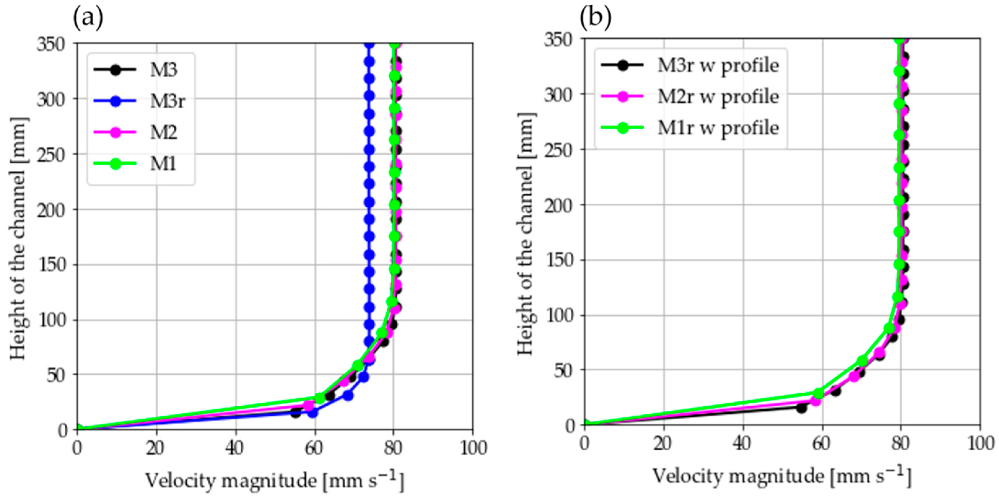
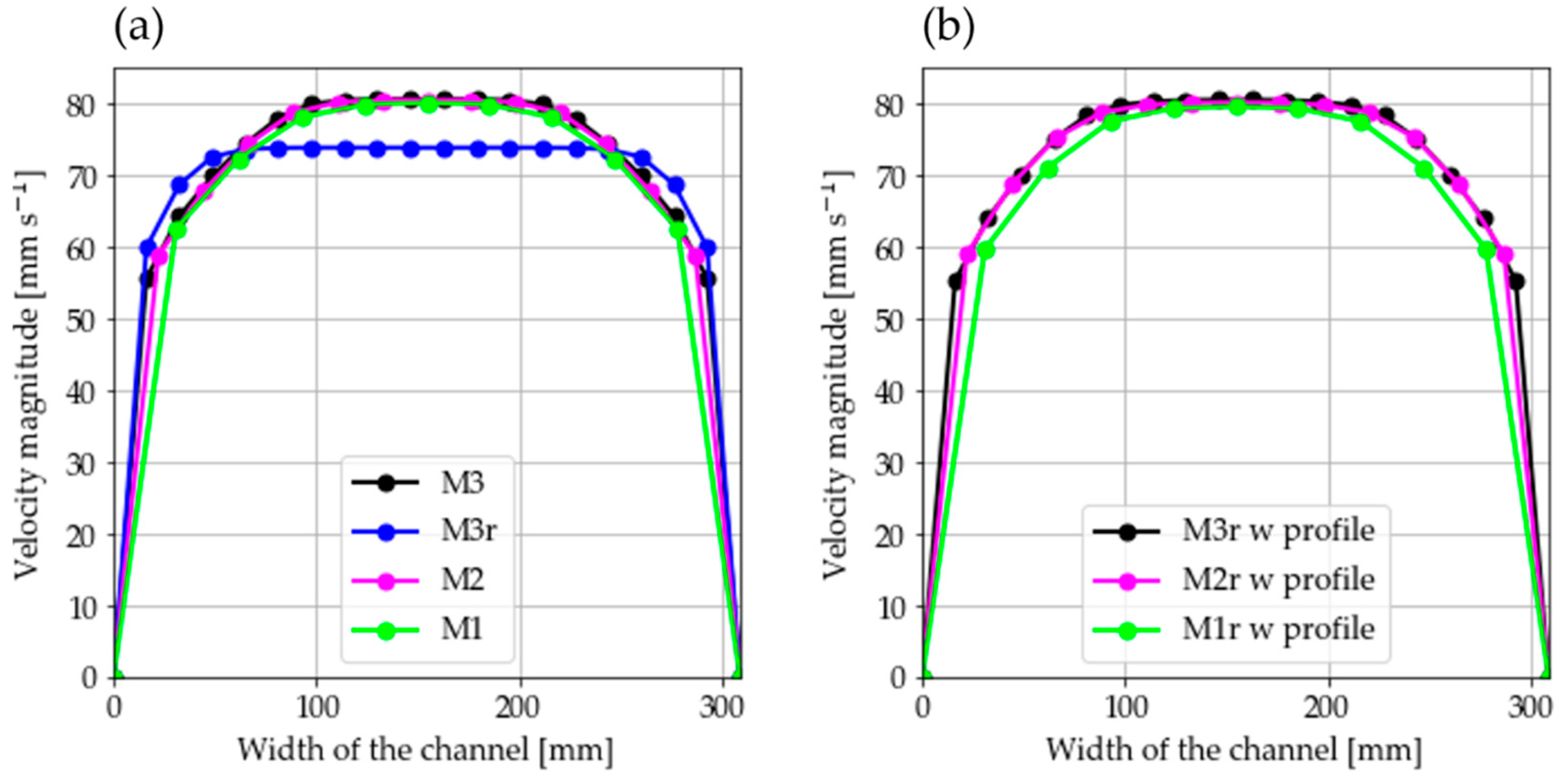
Vertical and horizontal fluid velocity profiles were plotted along the respective directions at the particle inlet location before particles were injected into domain. As shown in Figure 5 and Figure 6, both in the case of a whole domain and in the case of a reduced domain, all three mesh densities predict a similar velocity profile. The main difference is observed near the channel walls, where the coarse mesh underpredicts both the velocity gradient and the velocity magnitude. In comparison to the whole domain, significantly different velocity profiles are obtained on the meshes of the reduced domain. However, this can be corrected by applying the calculated velocity profiles on the fine mesh from the whole-domain case as an inlet boundary condition in the reduced-domain case.

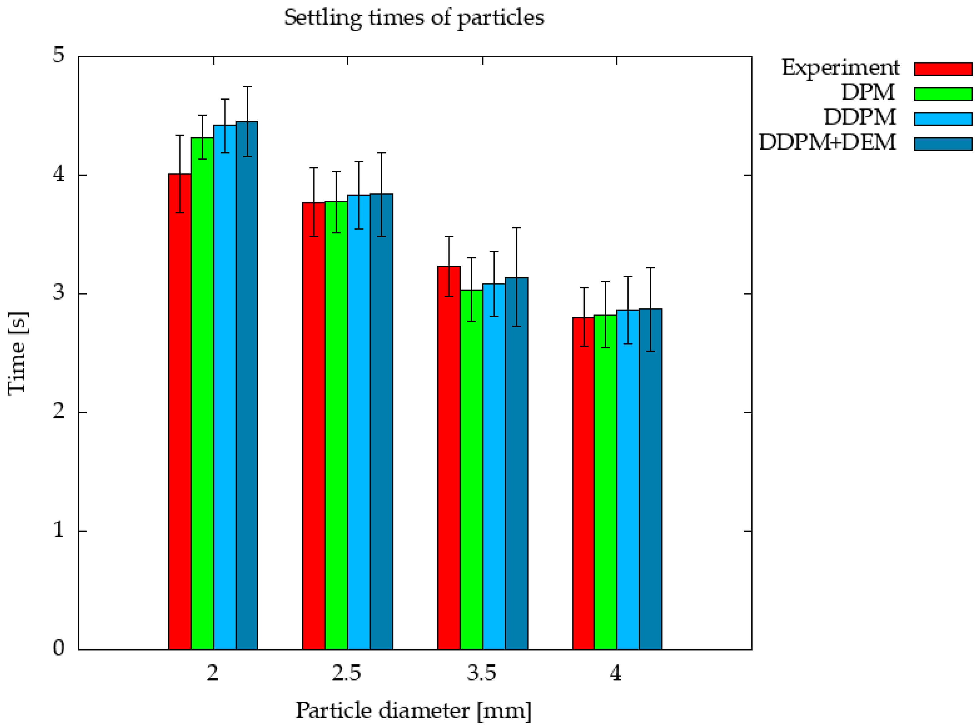
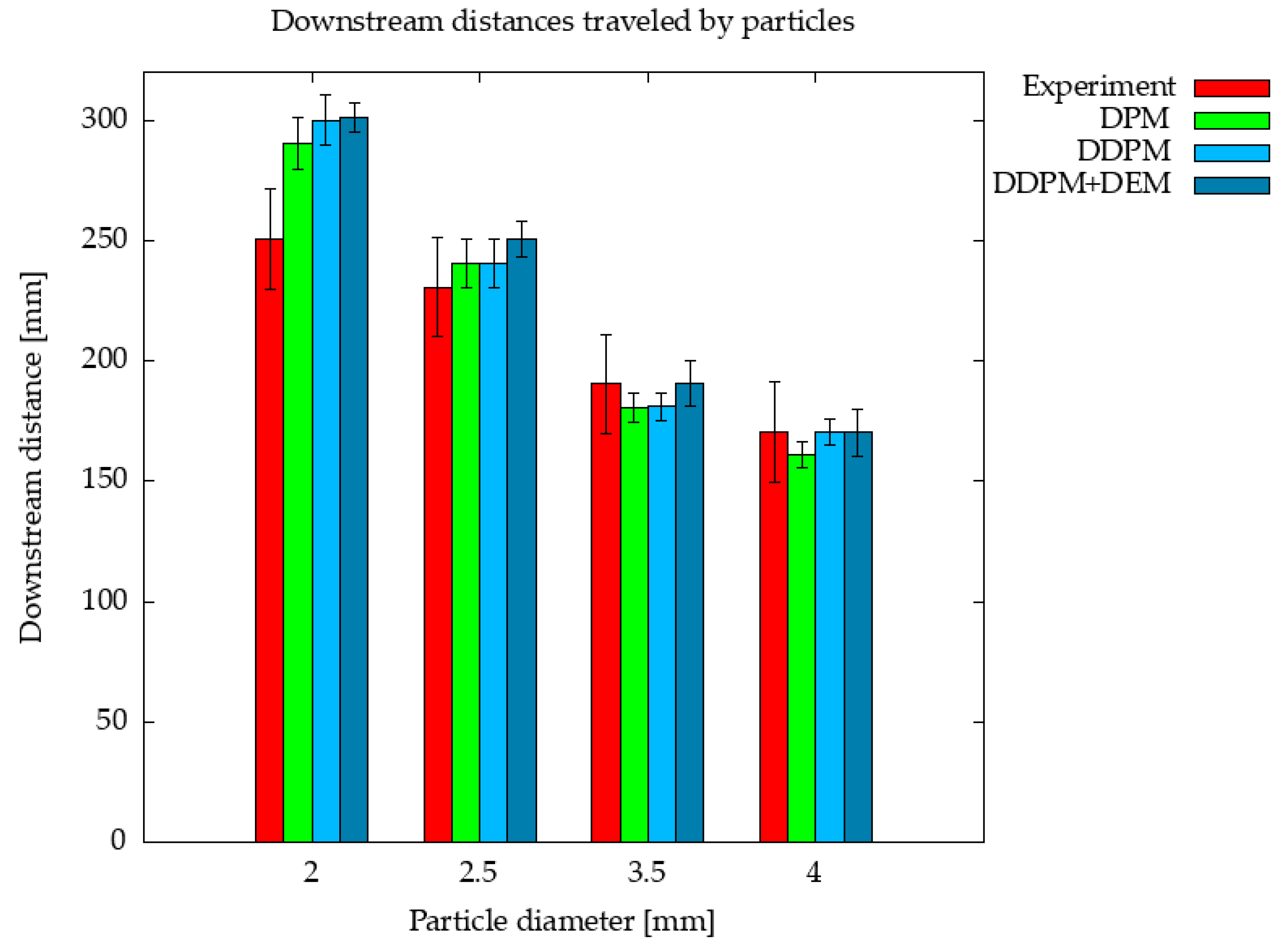
A comparison of calculated settling times obtained using three approaches and experimental values is presented in Figure 7. Satisfactory agreement was achieved for all three simulation approaches, except for the smallest particles with a diameter of 2 mm. A similar observation can be derived from the comparison of the downstream distance travelled by particles before settling on the bottom of the channel, as presented in Figure 8. Interaction between particles does not appear to be significant, as the DDPM approaches with and without inclusion of DEM produce similar results.

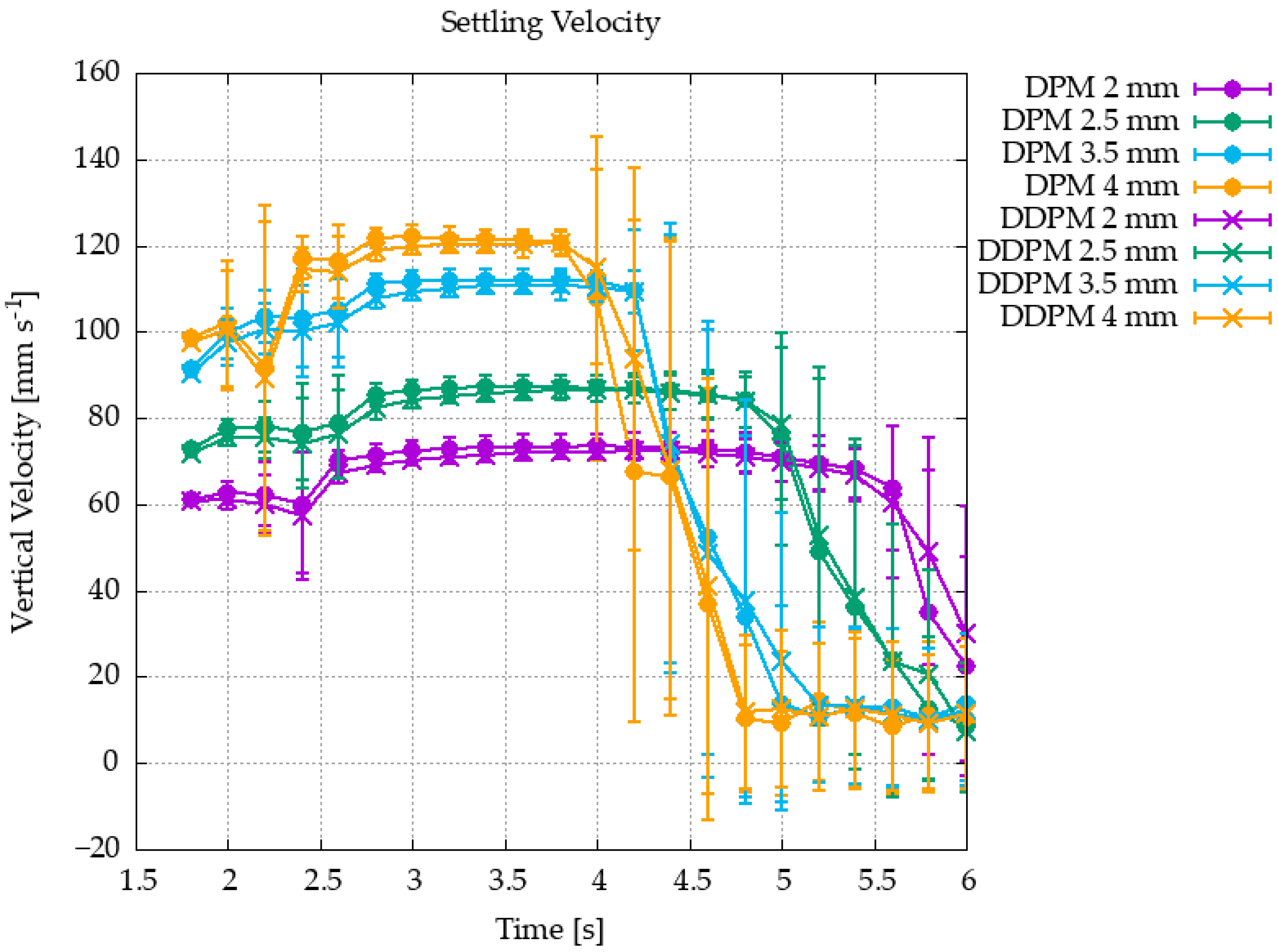
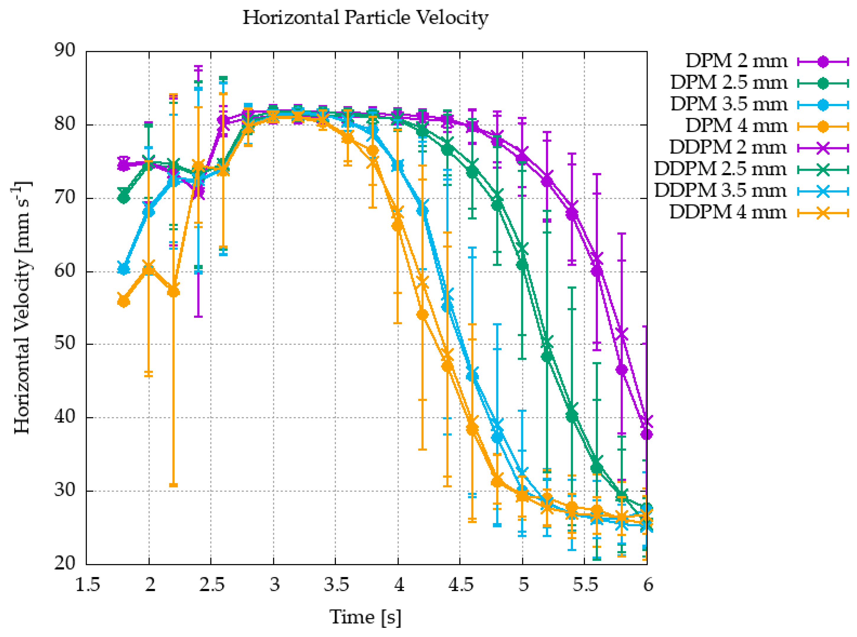
A more detailed comparison of the DPM and DDPM approaches is presented in Figure 9 and Figure 10, showing a time evolution of settling velocity and horizontal particle velocity, respectively. Minor differences can be observed, indicating that the point particle assumption of DPM is sufficient for treatment of mesoplastic particles in an open-channel flow.

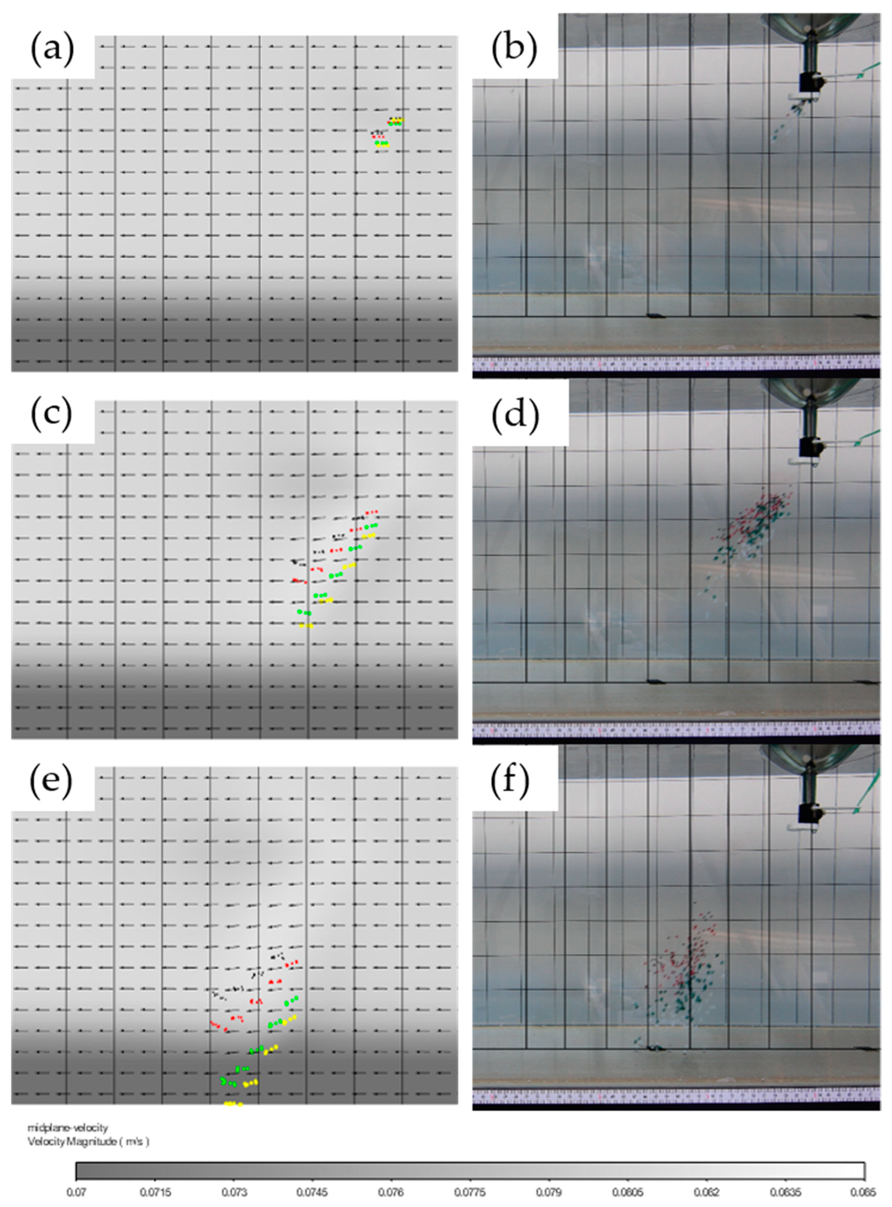
Figure 11 presents the propagation of a particle cloud as observed in the DPM simulation and the experiment at three different times. The color of the largest 4 mm particles is changed from white to yellow in the visualization of the simulation results for improved visibility. Additional vertical lines are drawn in the photos from the experiment that correspond to vertical lines drawn in the pictures from the simulation due to the difference in perspective. As shown in Figure 11, general agreement can be observed between simulation and experimental results, although with a noticeably tighter grouping of particles by size in the case of the simulation.

From both the experiment and simulations, it is evident that larger plastic particles settle more quickly than smaller particles, as expected, with the larger particles reaching a higher settling velocity. As shown in Figure 9, all particles reach terminal velocity (flattening of all curves for time evolution of velocity). Similarly, all particles reach the maximum horizontal velocity of the flow; as expected, smaller particles reach this velocity quicker than larger particles. Because larger particles reach the bottom of the channel sooner than smaller particles, their horizontal velocity also drops sooner. As shown by the velocity profile presented in Figure 5, the velocity adheres to a no-slip law (boundary condition); therefore, when particles approach the bottom of the channel, their velocity reduces accordingly. Figure 10 shows that settled particles retain some horizontal velocity in the simulation; however, this behavior is not observed in the experiment because an accurate particle–wall interaction was outside the scope of this study, and only the settling motion in the fluid was analyzed.

5. Conclusions

In this study the settling of mesoplastic particles of varying sizes in water was investigated. Settling times and downstream distance travelled by particles were measured experimentally. Numerical simulations were performed with three different approaches and compared to the experimental results. The computational effort was reduced by reducing the size of the domain (length of channel), and special care was taken to ensure the correct velocity profile was calculated at the position where particles were introduced into the domain, as the velocity profile of the water influences the velocity of the particles. The following conclusions can be drawn from this research:

(1)

Larger particles travel a shorter distance downstream, settle quicker and reach a higher terminal velocity than smaller particles, as expected based on previous research on this topic.

(2)

All investigated approaches to simulate settling of mesoplastic particles are appropriate and allow for a detailed investigation of particle motion. Interaction between particles is negligible and can be omitted, as it requires additional computational effort.

(3)

All presented modelling approaches produced tighter spatial grouping of particles compared to the experiment, indicating the need for future research on the topic particle motion modelling and evaluation of existing models.

The investigated approaches for simulation of particle settling in an open-channel flow can be used on a larger scale to predict the propagation of mesoplastics in rivers.

References

- Bermúdez, J.R.; Swarzenski, P.W. A microplastic size classification scheme aligned with universal plankton survey methods. MethodsX 2021, 8, 10–15. [Google Scholar] [CrossRef] [PubMed]
- Hartmann, N.B.; Hüffer, T.; Thompson, R.C.; Hassellöv, M.; Verschoor, A.; Daugaard, A.E. Are We Speaking the Same Language? Recommendations for a Definition and Categorization Framework for Plastic Debris. Environ. Sci. Technol. 2019, 53, 1039–1047. [Google Scholar] [CrossRef] [PubMed] [Green Version]
- Frias, J.P.G.L.; Nash, R. Microplastics: Finding a consensus on the definition. Mar. Pollut. Bull. 2018, 138, 145–147. [Google Scholar] [CrossRef] [PubMed]
- Wagner, M.; Lambert, S. (Eds.) Freshwater Microplastics; Springer International Publishing: Cham, Switzerland, 2018; Volume 58. [Google Scholar]
- GESAMP. Sources, Fate and Effects of Microplastics in the Marine Environment: A Global Assessment. 2015. Available online: www.imo.org (accessed on 18 October 2022).
- Sun, J.; Dai, X.; Wang, Q.; van Loosdrecht, M.C.M.; Ni, B.J. Microplastics in wastewater treatment plants: Detection, occurrence and removal. Water Res. 2019, 152, 21–37. [Google Scholar] [CrossRef]
- Čurlin, M.; Pušić, T.; Vojnović, B.; Vinčić, A. STEM Approach in Assessment of Microplastic Particles in Textile Wastewater. Teh. Vjesn. 2022, 29, 1777–1781. [Google Scholar] [CrossRef]
- Auta, H.S.; Emenike, C.U.; Fauziah, S.H. Distribution and importance of microplastics in the marine environment—A review of the sources, fate, effects, and potential solutions. Environ. Int. 2017, 102, 165–176. [Google Scholar] [CrossRef]
- Danopoulos, E.; Twiddy, M.; Rotchell, J.M. Microplastic contamination of drinking water: A systematic review. PLoS ONE 2020, 15, e0236838. [Google Scholar] [CrossRef]
- Eriksen, M.; Lebreton, L.C.; Carson, H.S.; Thiel, M.; Moore, C.J.; Borerro, J.C.; Reisser, J. Plastic Pollution in the World’s Oceans: More than 5 Trillion Plastic Pieces Weighing over 250,000 Tons Afloat at Sea. PLoS ONE 2014, 12, e111913. [Google Scholar] [CrossRef] [Green Version]
- Klein, S.; Dimzon, I.K.; Eubeler, J.; Knepper, T.P. Analysis, Occurrence, and Degradation of Microplastics in the Aqueous Environment; Springer: Cham, Switzerland, 2018; Volume 58. [Google Scholar]
- Lebreton, L.C.M.; Van Der Zwet, J.; Damsteeg, J.W.; Slat, B.; Andrady, A.; Reisser, J. River plastic emissions to the world’s oceans. Nat. Commun. 2017, 8, 15611. [Google Scholar] [CrossRef] [Green Version]
- Ren, Z.; Gui, X.; Xu, X.; Zhao, L.; Qiu, H.; Cao, X. Microplastics in the soil-groundwater environment: Aging, migration, and co-transport of contaminants—A critical review. J. Hazard. Mater. 2021, 419, 126455. [Google Scholar] [CrossRef]
- Schernewski, G.; Radtke, H.; Robbe, E.; Haseler, M.; Hauk, R.; Meyer, L.; Labrenz, M. Emission, Transport, and Deposition of visible Plastics in an Estuary and the Baltic Sea—A Monitoring and Modeling Approach. Environ. Manag. 2021, 68, 860–881. [Google Scholar] [CrossRef] [PubMed]
- Fatahi, M.; Akdogan, G.; Dorfling, C.; Van Wyk, P. Numerical study of microplastic dispersal in simulated coastal waters using cfd approach. Water 2021, 13, 3432. [Google Scholar] [CrossRef]
- Cook, S.; Chan, H.L.; Abolfathi, S.; Bending, G.D.; Schäfer, H.; Pearson, J.M. Longitudinal dispersion of microplastics in aquatic flows using fluorometric techniques. Water Res. 2020, 170, 115337. [Google Scholar] [CrossRef] [PubMed]
- Yu, Z.; Yao, W.; Loewen, M.; Li, X.; Zhang, W. Incipient Motion of Exposed Microplastics in an Open-Channel Flow. Environ. Sci. Technol. 2022, 56, 14498–14506. [Google Scholar] [CrossRef]
- Yi, Y.; Jia, W.; Yang, Y.; Zhang, S. Effects of diameter, density, and adhesiveness on settling velocity and drag coefficient of two sturgeon species eggs in flow. J. Hydraul. Res. 2022, 60, 229–239. [Google Scholar] [CrossRef]
- Roy, N.; Wijaya, K.P.; Götz, T.; Sundar, S. A mathematical model governing the short-range transport of microplastic particles in a lid-driven cavity with an obstacle. Commun. Nonlinear Sci. Numer. Simul. 2021, 101, 105893. [Google Scholar] [CrossRef]
- Fu, S.; Guo, X.Y.; Dong, L.H.; Sheng, K.; Sun, A. Numerical Simulation of Migration Laws of Dense Particle Flow in Pipelines. Int. J. Simul. Model. 2022, 21, 89–100. [Google Scholar] [CrossRef]
- Holjević, T.; Travaš, V.; Kranjčević, L.; Družeta, S. Analysis of Microplastic Particle Transmission. J. Marit. Transp. Sci. 2022, 4, 237–244. [Google Scholar] [CrossRef]
- Travaš, V.; Kranjčević, L.; Družeta, S.; Holjević, T.; Lučin, I.; Alvir, M.; Sikirica, A. Model gibanja čestica mikroplastike u nehomogenom i laminarnom polju brzine. Hrvatske Vode 2021, 29, 201–213. [Google Scholar]
- ANSYS. Ansys Fluent Theory Guide; ANSYS: Canonsburg, PA, USA, 2021. [Google Scholar]
- Morsi, S.A.; Alexander, A.J. An investigation of particle trajectories in two-phase flow systems. J. Fluid Mech. 1972, 55, 193–208. [Google Scholar] [CrossRef]
- Tsuji, Y.; Oshima, T.; Morikawa, Y. Numerical simulation of pneumatic conveying in the horizontal pipe. KONA Powder Part. J. 1985, 3, 38–51. [Google Scholar] [CrossRef]
- Dennis, S.C.R.; Singh, S.N.; Ingham, D.B. The steady flow due to a rotating sphere at low and moderate Reynolds numbers. J. Fluid Mech. 1980, 101, 257–279. [Google Scholar] [CrossRef]
- Mindlin, R.D.; Deresiewicz, H. Elastic Spheres in Contact Under Varying Oblique Forces. J. Appl. Mech. 1953, 20, 327–344. [Google Scholar] [CrossRef]
- Hertz, H. Über die Berührung fester elastischer Körper. J. Angew. Math. 1882, 92, 156–171. [Google Scholar] [CrossRef]
Figure 1.
Particle overlap definition.
Figure 2.
Hertz–Mindlin spring and dashpot system.
Figure 3.
HM 162 experimental flume: 1—water tank, 2—water outlet element, 3—sediment screen basket, 4—sediment pump, 5—PLC (switch box), 6—centrifugal pump, 7—flow rate sensor, 8—open-channel test section, 9—particle (sediment) inlet, 10—inclination adjustment element, 11—water inlet element.
Figure 4.
Detailed view of the particle inlet funnel.
Figure 5.
Vertical velocity profiles of water: (a) comparison between three mesh densities for the full domain and the fine mesh of the reduced domain; (b) comparison between three mesh densities of the reduced domain with a velocity profile boundary condition.
Figure 6.
Horizontal velocity profiles of water: (a) comparison between three mesh densities for the full domain and the fine mesh of the reduced domain; (b) comparison between three mesh densities of the reduced domain with a velocity profile boundary condition.
Figure 7.
Average settling times of plastic particles; error bars represent one standard deviation.
Figure 8.
Average downstream settling distance of plastic particles; error bars represent one standard deviation.
Figure 9.
Settling velocity of plastic particles; points represent average values, and error bars represent one standard deviation.
Figure 10.
Horizontal velocity of plastic particles; points represent average values, and error bars represent one standard deviation.
Figure 11.
Comparison of the particle cloud as observed in the experiment and the simulation using the DPM approach: (a) and (b) 0.5 s after the release of particles; (c) and (d) 1.5 s after the release of particles; (e) and (f) 2.5 s after the release of particles. Particles are colored by size as described in Table 1. Yellow color is used instead of white in the visualization of the simulation results.