Supplier Evaluation Considering Green Production Based on Probabilistic Linguistic Information

Abstract

The evaluation of manufacturing component suppliers is focused on economic indicators, with insufficient emphasis on green indicators and no consideration of the correlation between indicators. Firstly, indicators related to green production are incorporated into the supplier evaluation system. Then, for the problem that attributes in decision making can be divided into different categories and there are interrelationships between attributes of the same category, a multi-attribute decision-making (MADM) method based on the partitioned Maclaurin symmetric mean operator (PMSM) is proposed. Finally, the proposed MADM method was applied to the evaluation of component suppliers considering green production. Comparing popular decision methods with the newly proposed method for validation, it was demonstrated that the proposed multi-attribute decision method is highly flexible and versatile. Furthermore, the newly proposed aggregation operator can not only handle the correlation between multiple attributes, but also be converted to other general aggregation operators through parameter adjustment.

1. Introduction

On the backdrop of economic development and continuous technological innovation, civilization has leapt to a new level. Meanwhile, the problems of wasting resources and of environmental pollution are becoming more and more serious, posing a great challenge to the environment on which human beings depend for survival. As an important component under Industry 4.0, the manufacturing industry bears an important social responsibility for all of society. At the same time, with the introduction of governmental documents and global consensus agreements, the cost of environmental protection is also closely related to the economic performance of enterprises. Moreover, rising consumer awareness of environmental protection is driving companies to provide environmentally friendly products. Owing to the complexity and specialism of the manufacturing process and due to cost considerations, a large proportion of a manufacturing company’s components are outsourced to different suppliers, so manufacturing companies are extremely dependent on their suppliers. The environmental awareness and competence of suppliers are a key determinant of green production in companies. Delays in delivery or components being out of stock from major suppliers for environmental reasons would pose a significant risk to a company’s production and business activities. For example, one of Schaeffler’s needle roller suppliers had to stop production due to environmental problems, which caused most of the production lines of the downstream company to be suspended [1]. Therefore, apart from the decisions to be made when selecting suppliers, suppliers should also be evaluated and managed dynamically during the production process.

It is essential for manufacturers to update their supplier evaluation index systems to take into account indicators related to green production. Although some environmental indicators have been considered in previous supplier selections, many scholars have focused their research on ranking and selecting suppliers through evaluation methods before entering the production process. There are limitations to the applicability of the current research. The reason is that the current cooperation model starts with establishing a partnership with several qualified suppliers, and then with managing the suppliers with different priorities and measures during the production process [2]. Some scholars have studied the collaboration between manufacturing companies and equipment suppliers during the operational phase in order to improve manufacturing efficiency [3]. However, few studies have considered the evaluation and management of component suppliers during the manufacturing process.

The representation of evaluation information and the processing of evaluation information are important research questions for MADM. Due to the great uncertainty and ambiguity in the real decision-making environment, decision information is difficult to express through accurate figures. In addition, people prefer to use qualitative information to express their evaluation of things [4]. Therefore, considering the objective factors of the complexity of the decision-making environment and the subjective factors of human thinking and expression, DMs can express evaluation information more easily and precisely through qualitative information [5]. The numerical calculation of qualitative information is difficult, so the feature of quantifying qualitative information with the help of probabilistic linguistic information effectively deals with this problem.

For the evaluation of suppliers, previous studies have used the TOPSIS, VIKOR, DEA, and PROMETHEE methods [6,7,8,9]. However, this is all based on the premise that the evaluation indicators are independent of each other. In practice, there are often correlations between evaluation indicators, and the aggregation operator is an effective tool for considering attribute associations. In addition, aggregation operators are of great interest in decision making because they can provide specific scores for each alternative, in addition to the ranking results of the alternatives. Many aggregation operators have been studied and applied in MADM, such as the power average (PA), Heronian mean (HM), Bonferroni mean (BM), and Maclaurin symmetric mean (MSM) operators [10,11,12,13]. Although these operators can capture the interrelationships between attributes, there is also a problem in the actual decision-making process: attributes can be divided into several parts, and attributes in the same part have interrelationships with each other, while attributes in different parts do not have interrelationships with each other. For example, in the study by Yang et al., when considering how to make an asset allocation, the plan was to choose from five alternative sectors: real estate, energy, gold, the stock market, and artificial intelligence companies [14]. The five main attributes of market potential, growth potential, total risk–loss capital, amount of interest received, and inflation, were considered, and these attributes were divided into two groups based on the interrelationship between the attributes. Yang et al. solved this problem by using the partitioned Bonferroni mean (PBM) operator [14]. However, the PBM operator only captures the interrelationship between two attributes and is not ideal for cases where there are interrelationships between multiple attributes. Inspired by the PBM operator, Liu et al. and Bai et al. both proposed the PMSM operator, which they applied to intuitionistic fuzzy sets and Q-order orthogonal fuzzy sets, respectively [15,16].

The supplier evaluation problem based on green production is a typical MADM problem, and research on this problem is of significant value for the construction of green supply chains. This paper therefore establishes a decision method for solving the supplier evaluation problem by using probabilistic linguistic information, allowing decision makers to better express their own evaluation information and quantifying qualitative information, and the PMSM operator allowing a more comprehensive treatment of the relationships between attributes. The next sections of this paper are as follows. Section 2 gives a review of the relevant literature; in Section 3, a supplier evaluation method based on the probabilistic linguistic terms set (PLS) is proposed; and Section 4 presents a case study and validation of the proposed method and discusses the influence of parameters. The final section gives the conclusions of the paper and directions that can be further explored in the future.

2. Literature Review

In this paper, we focus on the green production evaluation of manufacturing component suppliers, using probabilistic linguistic information as evaluation information and PLWPMSM to deal with the interrelationships between attributes. The literature review has three main components: supplier evaluation, probabilistic linguistic information, and the aggregation operator.

2.1. Supplier Evaluation Manufacturing

In previous supplier evaluations, factors such as product quality, delivery time, and price have been the core indicators in supplier evaluations [17]. For example, quality, delivery, and historical performance have been identified as the three most important indicators. Lin et al. mainly considered quality, delivery time, and price as indicators in their recent study [18]. While these indicators play a large role in the assessment of suppliers, they lack the quantification of environment-related indicators, especially with the release of some international certification standards related to the environment by some developed countries and organizations, such as ISO 14000, ISO 14040, and ISO 14044, which consider the product life cycle [19]. Although green production-related indicators have been considered previously in the selection of suppliers, the screening process is integrated with the actual development and environmental capability of the suppliers. Tseng et al. used a printed circuit board manufacturing company as an example to explore green supply chain management, and added environmental performance to the supplier evaluation criteria in order to improve the environmental benefits of the company [20]. Pech and Vaněček also pointed out that firms differ in their supplier performance management characteristics [21]. When selecting a supplier, enterprises should not only consider the supplier’s delivery capability, product quality, and price, as well as the supplier’s position in the industry, but also whether the supplier has taken effective measures to conserve resources and to protect the environment. This paper designs a framework to establish an evaluation index system that considers green production, incorporating the current status of green production of an enterprise’s partner suppliers.

2.2. Probabilistic Linguistic Information

PLS is based on the hesitant fuzzy language set (HFLS), which overcomes the disadvantage that while HFLS allows decision makers to express multiple possible values, it cannot assign different weights to multiple possible values. It also has the advantage of taking qualitative decision information and quantifying it. Pang et al. first proposed the idea of PLS and gave the basic operation rules, but the computational process tends to exceed the bounds [22]. So, Gou et al. proposed a new transformation function to solve this problem, which laid a solid foundation for further research on PLS [23]. Subsequently, other scholars have conducted research on preference relations, distance formulas, similarity formulas, etc., enriching the theory of PLS [24,25,26,27,28,29]. In addition, a considerable number of scholars have proposed new approaches to solve MADM by combining PLS and related methods; for example, Zhang and Xing proposed an extended TOPSIS approach to solve MADM by combining PLS and TOPSIS, which combines the VIKOR method with PLS to solve green supply chain-related problems [30]. Wu and Liao addressed the quality function deployment problem through the PLS ORESTE approach [31]. Mao et al. combined ELECTRE with TOPSIS, in the context of PLS, to propose a solution for Fintech company selection [32]. In addition, considering the limited rationality of decision makers, Liu and You considered extending the TODIM approach to PLS to solve the MADM problem [33]. Liu and Li developed a new approach to solve the MADM problem by extending MULTIMOORA to PLS, based on prospect theory [29]. Wu et al. proposed a Borda rule-based PL-MULTIMOORA method to select karaoke TV brands for investments [34]. PLS has a wide range of applications in MADM, but the current research considering associations between multiple attributes in a probabilistic language setting has some shortcomings.

2.3. Aggregation Operator

Pang et al. gave the forms of geometric and averaging operators in the context of a probabilistic language set [22]. Bai et al. redefined the PLS averaging operator and PLS geometric operator based on the new operation rules proposed by Gou [23,28]. Although the proposed PLWA operator and PLWG operator can help the decision-making process to a large extent, he ignored the variation among attributes. To address this problem, Kobina et al. represented the interrelationships between attributes through the mutual support of probabilistic linguistic power averaging (PLPA) operators [35]. By introducing the Bonferroni mean operator in a probabilistic linguistic ensemble, Liang et al. proposed the probabilistic linguistic Bonferroni mean (PLBM) operator to express the correlation between two attributes [36]. Considering that the relationship between two attributes is also the Heronian mean operator, Feng et al. used it in combination with other methods in order to select a suitable waste water treatment solution [37]. For capturing the interrelationships between multiple attributes, the Maclaurin symmetric mean (MSM) operator proposed by Maclaurin has great advantages. The MSM operator can handle the case where there are correlations between multiple attributes by scaling the parameter k. Liu et al. combined the probabilistic language set with the MSM operator and proposed the PLMSM operator to solve the case where there are multiple correlations, followed by a generalized MSM operator with stronger generality [38,39,40]. Although there were good results in the study of aggregation operators under probabilistic language sets, previous studies have been too hypothetical, highlighting the existence of interrelationships between all attributes and ignoring the cases where some attributes do not have interrelationships with each other.

Based on the analysis, it can be concluded that the evaluation of suppliers in terms of quality, price, and delivery times alone is no longer sufficient to meet practical needs. Indicators related to green production need to be included in the evaluation system. Scientific expressions were chosen to express the evaluation of information, and the correlation between attributes was taken into account in the calculation of the results in order to achieve more scientific results. Finally, suppliers were assigned priorities and market shares based on the evaluation results.

3. Methodology

This section presents the PLPMSM operator and the PLWPMSM operator by improving the PMSM operator to suit the probabilistic language environment.

3.1. Partitioned Maclaurin Symmetric Mean Aggregation Operator

Definition 1.

Assuming that$Q=\left\{{\tilde{\alpha }}_1,{\tilde{\alpha }}_2,\dots ,{\tilde{\alpha }}_n\right\}$is a set of non-negative real numbers, it can be divided into different parts,$B_1,B_2,\dots ,B_m$, where ${\tilde{B}}_i\cap {\tilde{B}}_j=\varnothing$and ${\displaystyle \underset{\gamma =1}{\overset{m}{\cup }}{\tilde{B}}_{\gamma }}=Q$. The PMSM operator is defined as:

$$PMS{M}^{({\kappa }_1,\dots ,{\kappa }_m)}\left({\tilde{\alpha }}_1,{\tilde{\alpha }}_2,\dots ,{\tilde{\alpha }}_n\right)=\frac{1}{m}{{\displaystyle \sum _{\gamma =1}^m\left(\frac{{\displaystyle \sum _{1\le i_1<\dots <i_{\kappa }\le B_{\gamma }}\left({\displaystyle \prod _{j=1}^{\kappa }{\alpha }_i{}_{{}_j}}\right)}}{C_{B_{\gamma }}^{\kappa }}\right)}}^{1/{\kappa }_{\gamma }}$$

(1)

where ${\kappa }_{\gamma }$is the parameter in the partition $B_{\gamma }$, the range of the $\kappa$value is $\left[1,\left|B_{\gamma }\right|\right]$, $\left|B_{\gamma }\right|$indicates the number of input arguments in the partition, $B_{\gamma }$$\left(i_1,i_2,\dots ,i_{{\kappa }_{\gamma }}\right)$traverses the overall ${\kappa }_r$-tuple different combinations of $\left(1,2,\dots ,\left|B_{\gamma }\right|\right)$; $C_{\left|B_{\gamma }\right|}^{{\kappa }_{\gamma }}$denotes the binomial coefficient, and $C_{\left|B_{\gamma }\right|}^{{\kappa }_{\gamma }}=\frac{n!}{{\kappa }_{\gamma }!\left(n-{\kappa }_{\gamma }\right)!}$.

The $PMS{M}^{({\kappa }_1,{\kappa }_{2,}\dots ,{\kappa }_m)}$ has the following properties:

(1)

$PMS{M}^{\left({\kappa }_1,{\kappa }_{2,}\dots ,{\kappa }_m\right)}\left(0,0,\dots ,0\right)=0$ and $PMS{M}^{\left({\kappa }_1,{\kappa }_{2,}\dots ,{\kappa }_m\right)}\left(\tilde{a},\tilde{a},\dots ,\tilde{a}\right)=\tilde{a}$;

(2)

$PMS{M}^{\left({\kappa }_1,{\kappa }_{2,}\dots ,{\kappa }_m\right)}\left({\tilde{a}}_1,{\tilde{a}}_2,\dots ,{\tilde{a}}_n\right)\le PMS{M}^{\left({\kappa }_1,{\kappa }_{2,}\dots ,{\kappa }_m\right)}\left({\tilde{b}}_1,{\tilde{b}}_2,\dots ,{\tilde{b}}_n\right)$ if ${\tilde{a}}_i\le {\tilde{b}}_i$ for all $i$;

(3)

$\underset{i}{\min }\left\{{\tilde{a}}_i\right\}\le PMS{M}^{\left({\kappa }_1,{\kappa }_{2,}\dots ,{\kappa }_m\right)}\left({\tilde{a}}_1,{\tilde{a}}_2,\dots ,{\tilde{a}}_n\right)\le \underset{i}{\max }\left\{{\tilde{a}}_i\right\}$.

3.2. Probabilistic Linguistic Partitioned Maclaurin Symmetric Mean Aggregation Operator

Definition 2.

Let$\tilde{T}s\left(\pi \right)=\left\{\tilde{T}{s}_i^{\left(\tau \right)}\left({\pi }_i^{\left(\tau \right)}\right)|\tau =1,2,\dots ,\#\tilde{T}{s}_{\mathrm{i}}\left(\pi \right)\right\}\left(i=1,2,\dots ,n\right)$be n PLS, where $\tilde{T}{s}_i^{\left(\tau \right)}$and${\pi }_i^{\left(\tau \right)}$are the kth LT and its probability, respectively, in$\tilde{T}{s}_i\left(\pi \right)$, and$PLPMSM$is defined as:

$$PLPMS{M}^{\left(k\right)}\left(T{s}_1\left(\pi \right),T{s}_2\left(\pi \right),\dots ,T{s}_n\left(\pi \right)\right)=\frac{1}{m}\underset{\gamma =1}{\overset{m}{\oplus }}{\left(\frac{\underset{1\le i_1<\dots <i_{\kappa }\le {\tilde{B}}_r}{\oplus }\left(\underset{j=1}{\overset{\kappa }{\otimes }}Ts{\left(\pi \right)}_{i_j}\right)}{C_{B_{\gamma }}^{\kappa }}\right)}^{\frac{1}{\kappa }}$$

(2)

where$m$denotes the number of partitions, $\kappa \in \left(1,2,\dots ,n\right)$$\left(i_1,i_2,\dots ,i_{\kappa }\right)$traverses all $\kappa -tuple$combinations of $\left(1,2,\dots ,n\right)$, and $C_n^{\kappa }$is the binomial coefficient; the $PLPMS{M}^{\left(\kappa \right)}$is called the $PLPMSM$operator.

Theorem 1.

Let$\tilde{T}{s}_i\left(\pi \right)=\left\{\tilde{T}{s}_i^{\left(\tau \right)}\left({\pi }_i^{\left(\tau \right)}\right)|\tau =1,2,\dots ,\#\tilde{T}{s}_{\mathrm{i}}\left(\pi \right)\right\}\left(i=1,2,\dots ,n\right)$be n PLS; then, the aggregated result by Definition 2 is:

$$\begin{array}{l}PLPMS{M}^{\left(\kappa \right)}\left(T{s}_1\left(\pi \right),T{s}_2\left(\pi \right),\dots ,T{s}_n\left(\pi \right)\right)=\frac{1}{m}\underset{\gamma =1}{\overset{m}{\oplus }}{\left(\frac{\underset{1\le i_1<\dots <i_{\kappa }\le B_{\gamma }}{\oplus }\left(\underset{j=1}{\overset{\kappa }{\otimes }}Ts{\left(\pi \right)}_{i_j}\right)}{C_{B_{\gamma }}^{\kappa }}\right)}^{\frac{1}{\kappa }}\\ ={{\displaystyle \cup }}_{{\xi }_1^{(\tau )}\in g\left(T{s}_1\left(\pi \right)\right),{\xi }_2^{(\tau )}\in g\left(T{s}_2\left(\pi \right)\right),\dots ,{\xi }_{B_{\gamma }}^{(\tau )}\in g\left(T{s}_{B_{\gamma }}\left(\pi \right)\right)}\\ \left\{g^{-1}\left(1-{\left(\underset{\gamma =1}{\overset{m}{\Pi }}\left(1-{\left(1-{\left(\underset{1\le i_1<\dots <i_{{\kappa }_{\gamma }}\le \left|B_{\gamma }\right|}{\Pi }\left(1-\left(\underset{j=1}{\overset{\kappa }{\Pi }}{\xi }_{i_j}^{(\tau )}\right)\right)\right)}^{C_{B_r}^{\kappa }}\right)}^{\frac{1}{\kappa }}\right)\right)}^{\frac{1}{m}}\right)\left(\underset{\gamma =1}{\overset{m}{\Pi }}\underset{1\le i_1<\dots <i_{{\kappa }_{\gamma }}\le \left|B_{\gamma }\right|}{\Pi }\underset{j=1}{\overset{\kappa }{\Pi }}{\pi }_{i_j}^{(\tau )}\right)\right\}\end{array}$$

(3)

Refer to Appendix B for the detailed proof of Theorem 1.

Theorem 2.

(Commutativity) Suppose$\tilde{T}{s}^{\prime }=\left\{\tilde{T}{s^{\prime }}_1\left(\pi \right),\tilde{T}{s^{\prime }}_2\left(\pi \right),\dots ,\tilde{T}{s^{\prime }}_n\left(\pi \right)\right\}$and$\tilde{T}s=\left\{\tilde{T}{s}_1\left(\pi \right),\tilde{T}{s}_2\left(\pi \right),\dots ,\tilde{T}{s}_n\left(\pi \right)\right\}$are two probabilistic linguistic sets, where$\tilde{T}{s}^{\prime }$is any of the permutations of the elements in $\tilde{T}s$.

$$PLPMSM\left(T{s}_1\left(\pi \right),T{s}_2\left(\pi \right),\dots ,T{s}_n\left(\pi \right)\right)=PLPMSM\left(T{s}_1{}^{\prime }\left(\pi \right),T{s}_2{}^{\prime }\left(\pi \right),\dots ,T{s}_n{}^{\prime }\left(\pi \right)\right)$$

(4)

Refer to Appendix B for the detailed proof of Theorem 2.

Next, we explore to improve PLPMSM operator parameters $\kappa$ and $B$, and some special cases are introduced.

When $m=1$, the proposed PLPMSM operator becomes the PLMSM operator shown below:

$$\begin{array}{l}PLPMSM={\left(\frac{\underset{1\le i_1<\dots <i_{\kappa }\le B_r}{\oplus }\left(\underset{j=1}{\overset{\kappa }{\otimes }}T{s}_{i_j}\right)}{C_{B_{\gamma }}^{\kappa }}\right)}^{\frac{1}{\kappa }}\\ ={{\displaystyle \cup }}_{{\gamma }_1^{(t)}\in g\left(L{S}_1\left(p\right)\right),{\gamma }_2^{(t)}\in g\left(L{S}_2\left(p\right)\right),\dots ,{\gamma }_{h_r}^{(t)}\in g\left(L{S}_{h_r}\left(p\right)\right)}\left\{\begin{array}{l}{g}^{-1}{\left(1-{\left(\underset{1\le i_1<\dots <i_{k_{\gamma }}\le \left|B_{\gamma }\right|}{\Pi }\left(1-\left(\underset{j=1}{\overset{\kappa }{\Pi }}{\xi }_{i_j}^{(\tau )}\right)\right)\right)}^{C_{B_{\gamma }}^{\kappa }}\right)}^{\frac{1}{\kappa }}\\ \left(\underset{1\le i_1<\dots <i_{{\kappa }_{\gamma }}\le \left|B_{\gamma }\right|}{\Pi }\underset{j=1}{\overset{\kappa }{\Pi }}{\pi }_{i_j}^{(\tau )}\right)\end{array}\right\}\\ =PLPMSM\end{array}$$

(5)

When $\kappa =1$, the PLPMSM operator is simplified to the probabilistic linguistic partitioned mean (PLPM) operator, given as follows:

$$\begin{array}{cc}\hfill PLPMSM& =\frac{1}{m}\underset{\gamma =1}{\overset{m}{\oplus }}{\left(\frac{\underset{1\le i_1<\dots <i_{\kappa }\le B_{\gamma }}{\oplus }\left(Ts{\left(\pi \right)}_{i_j}\right)}{C_{B_{\gamma }}^1}\right)}^{\frac{1}{B_{\gamma }}}\hfill \\ & ={{\displaystyle \cup }}_{{\xi }_1^{(\tau )}\in g\left(T{s}_1\left(\pi \right)\right),{\xi }_2^{(\tau )}\in g\left(T{s}_2\left(\pi \right)\right),\dots ,{\xi }_{B_{\gamma }}^{(\tau )}\in g\left(\tilde{T}{s}_{{\tilde{B}}_{\gamma }}\left(\pi \right)\right)}\left\{g^{-1}\left(\begin{array}{l}1-{\left(\underset{\gamma =1}{\overset{m}{\Pi }}\left(1-\left(1-{\left(\underset{i=1}{\overset{B_{\gamma }}{\Pi }}\left(1-{\xi }_{i_j}^{(\tau )}\right)\right)}^{C_{h_r}^k}\right)\right)\right)}^{\frac{1}{m}}\\ \left(\underset{\gamma =1}{\overset{m}{\Pi }}\underset{i=1}{\overset{B_{\gamma }}{\Pi }}{\pi }_{i_j}^{(\tau )}\right)\end{array}\right)\right\}\hfill \\ & ={{\displaystyle \cup }}_{{\gamma }_1^{(t)}\in g\left(L{S}_1\left(p\right)\right),{\gamma }_2^{(t)}\in g\left(L{S}_2\left(p\right)\right),\dots ,{\gamma }_{h_r}^{(t)}\in g\left(L{S}_{h_r}\left(p\right)\right)}\left\{g^{-1}\left(\begin{array}{l}1-{\left(\underset{\gamma =1}{\overset{m}{\Pi }}{\left(\underset{i=1}{\overset{B_{\gamma }}{\Pi }}\left(1-{\xi }_{i_j}^{(\tau )}\right)\right)}^{C_{h_r}^k}\right)}^{\frac{1}{m}}\\ \left(\underset{\gamma =1}{\overset{m}{\Pi }}\underset{i=1}{\overset{B_{\gamma }}{\Pi }}{\pi }_{i_j}^{(\tau )}\right)\end{array}\right)\right\}\hfill \end{array}$$

(6)

When $\kappa =2$, the PLPMSM operator is simplified to the probabilistic linguistic partitioned Bonferroni mean (PLPBM) operator ($p=1,q=1$):

$$\begin{array}{l}PLPMS{M}^{\left(2\right)}=\frac{1}{m}\underset{\gamma =1}{\overset{m}{\oplus }}{\left(\frac{\underset{1\le i_1<\dots <i_{\kappa }\le B_{\gamma }}{\oplus }\left(\underset{j=1}{\overset{2}{\otimes }}T{s}_{i_j}\right)}{C_{B_{\gamma }}^2}\right)}^{\frac{1}{2}}\\ ={{\displaystyle \cup }}_{{\xi }_1^{(\tau )}\in g\left(T{s}_1\left(\pi \right)\right),{\xi }_2^{(\tau )}\in g\left(T{s}_2\left(\pi \right)\right),\dots ,{\xi }_{B_{\gamma }}^{(\tau )}\in g\left(\tilde{T}{s}_{{\tilde{B}}_{\gamma }}\left(\pi \right)\right)}\\ \left\{g^{-1}\left(1-{\left(\underset{\gamma =1}{\overset{m}{\Pi }}\left(1-{\left(1-{\left(\underset{1\le i_1<\dots <i_{{\kappa }_{\gamma }}\le \left|B_{\gamma }\right|}{\Pi }\left(1-\left(\underset{j=1}{\overset{2}{\Pi }}{\xi }_{i_j}^{(\tau )}\right)\right)\right)}^{C_{B_r}^2}\right)}^{\frac{1}{2}}\right)\right)}^{\frac{1}{m}}\right)\left(\underset{\gamma =1}{\overset{m}{\Pi }}\underset{1\le i_1<\dots <i_{{\kappa }_{\gamma }}\le \left|{\tilde{B}}_{\gamma }\right|}{\Pi }\underset{j=1}{\overset{2}{\Pi }}{\pi }_{i_j}^{(\tau )}\right)\right\}\end{array}$$

(7)

3.3. Probabilistic Linguistic Weighted Partitioned Maclaurin Symmetric Mean Aggregation Operator

In this section, PLWPMSM is presented in Definition 2, where it is assumed that the weights of all attributes are the same. However, in real decision making, each attribute or decision maker has a different weight. Therefore, it is necessary to consider the case where each variable has its own weight. Assuming that each variable has a corresponding weight, the PLWPMSM operator is shown below:

Definition 3.

Suppose that$\tilde{T}s\left(\pi \right)=\left\{\tilde{T}{s}_i^{\left(\tau \right)}\left({\pi }_i^{\left(\tau \right)}\right)|\tau =1,2,\dots ,\#\tilde{T}{s}_{\mathrm{i}}\left(\pi \right)\right\}\left(i=1,2,\dots ,n\right)$is a set of n probabilistic languages, and$\omega ={\left({\omega }_1,{\omega }_2,\dots ,{\omega }_{\mathrm{n}}\right)}^T$is the corresponding weight vector and satisfies${\omega }_i\in \left[0,1\right]$,$i=1,2,\dots ,n$and${\displaystyle \sum _{j=1}^n{\omega }_j}=1$.

$$WPLPMSM\left(T{s}_1\left(\pi \right),T{s}_2\left(\pi \right),\dots ,T{s}_n\left(\pi \right)\right)=\frac{1}{m}\underset{\gamma =1}{\overset{m}{\oplus }}{\left(\frac{\underset{1\le i_1<\dots <i_{\kappa }\le B_{\gamma }}{\oplus }\left(\underset{j=1}{\overset{\kappa }{\otimes }}{\omega }_{i_j}Ts{\left(\pi \right)}_{i_j}\right)}{C_{B_{\gamma }}^{\kappa }}\right)}^{\frac{1}{\kappa }}$$

(8)

where $m$denotes the number of partitions, $\kappa \in \left(1,2,\dots ,n\right)$$\left(i_1,i_2,\dots ,i_{\kappa }\right)$traverses all $\kappa$-tuple combinations of $\left(1,2,\dots ,n\right)$, where $0\le \omega \le 1$and ${\displaystyle \sum _{i=1}^n{\omega }_i}=1$,$C_n^{\kappa }$is the binomial coefficient, whose expression is$C_{B_{\gamma }}^{\kappa }=\frac{B_{\gamma }!}{\kappa !\left(B_{\gamma }-\kappa \right)}$, and the $PLPMS{M}^{(\kappa )}$is called the $PLPMSM$operator.

Theorem 3.

Let$\tilde{T}s\left(\pi \right)=\left\{\tilde{T}{s}_i^{\left(\tau \right)}\left({\pi }_i^{\left(\tau \right)}\right)|\tau =1,2,\dots ,\#\tilde{T}{s}_{\mathrm{i}}\left(\pi \right)\right\}\left(i=1,2,\dots ,n\right)$be n PLS and$w =$$\left(w_1,w_2,\right.$${\left.\dots ,w_n\right)}^T$be the weight vector of$\tilde{T}{s}_i\left(\pi \right)$with $w_i\in \left[0,1\right]$,$i=1,2,\dots ,n$, and${\displaystyle {\sum }_{\mathrm{i}=1}^{\mathrm{n}}{w}_i}=1$.Then, the aggregated result by Definition 3 is:

$$\begin{array}{l}WPLPMSM\\ =\underset{{\xi }_1^{(\tau )}\in g\left(T{s}_1\left(\pi \right)\right),{\xi }_2^{(\tau )}\in g\left(T{s}_2\left(\pi \right)\right),\dots ,{\xi }_{B_{\gamma }}^{(\tau )}\in g\left(T{s}_{{\tilde{B}}_{\gamma }}\left(\pi \right)\right)}{{\displaystyle \cup }}\left\{g^{-1}\left(1-{\left(\underset{\gamma =1}{\overset{m}{\Pi }}\left(1-{\left(1-{\left(\begin{array}{l}\underset{1\le i_1<\dots <i_{\kappa }\le \left|B_{\gamma }\right|}{\Pi }\\ \left(1-\left(\underset{j=1}{\overset{\kappa }{\Pi }}\left(1-{\left(1-{\xi }_{i_j}^{(\tau )}\right)}^{{\omega }_{i_j}}\right)\right)\right)\end{array}\right)}^{\frac{1}{C_{B_{\gamma }}^{\kappa }}}\right)}^{\frac{1}{\kappa }}\right)\right)}^{\frac{1}{m}}\right)\right.\\ \left.\left(\underset{\gamma =1}{\overset{m}{\Pi }}\underset{1\le i_1<\dots <i_{\kappa }\le \left|B_{\gamma }\right|}{\Pi }\underset{j=1}{\overset{\kappa }{\Pi }}{\pi }_{i_j}^{(\tau )}\right)\right\}\end{array}$$

(9)

Theorem 4.

(Commutativity) Given that$T{s}^{\prime }=\left\{T{s^{\prime }}_1\left(\pi \right),T{s^{\prime }}_2\left(\pi \right),\dots ,T{s^{\prime }}_n\left(\pi \right)\right\}$and$\left\{T{s}_1\left(\pi \right),\right.T{s}_2\left(\pi \right),\left.\dots ,T{s}_n\left(\pi \right)\right\}$are two probabilistic linguistic sets, where$T{s}^{\prime }$is any permutation of the elements in$LS$

$$PLWPMSM\left(T{s}_1\left(\pi \right),T{s}_2\left(\pi \right),\dots ,T{s}_n\left(\pi \right)\right)=PLWPMSM\left(T{s}_1{}^{\prime }\left(\pi \right),T{s}_2{}^{\prime }\left(\pi \right),\dots ,T{s}_n{}^{\prime }\left(\pi \right)\right)$$

(10)

The proofs of Theorems 3 and 4 are similar to Theorems 1 and 2, so they are omitted here.

Finally, some special examples of the IFWPMSM operator are discussed.

When $m=1$, the PLWPMSM operator is equivalent to the PLWMSM operator:

$$\begin{array}{l}PLWPMSM={\left(\frac{\underset{1\le i_1<\dots <i_{\kappa }\le B_{\gamma }}{\oplus }\left(\underset{j=1}{\overset{\kappa }{\otimes }}{\omega }_{i_j}Ts{\left(\pi \right)}_{i_j}\right)}{C_{{\tilde{B}}_{\gamma }}^{\kappa }}\right)}^{\frac{1}{\kappa }}\\ ={{\displaystyle \cup }}_{{\xi }_1^{(\tau )}\in g\left(T{s}_1\left(\pi \right)\right),{\xi }_2^{(\tau )}\in g\left(T{s}_2\left(\pi \right)\right),\dots ,{\xi }_{B_{\gamma }}^{(\tau )}\in g\left(\tilde{T}{s}_{{\tilde{B}}_{\gamma }}\left(\pi \right)\right)}\\ \left\{g^{-1}{\left(1-{\left(\underset{1\le i_1<\dots <i_{\kappa }\le \left|B_{\gamma }\right|}{\Pi }\left(1-\left(\underset{j=1}{\overset{\kappa }{\Pi }}{\left(1-{\xi }_{i_j}^{(\tau )}\right)}^{w_{i_j}}\right)\right)\right)}^{C_{B_{\gamma }}^{\kappa }}\right)}^{\frac{1}{\kappa }}\left(\underset{1\le i_1<\dots <i_{\kappa }\le \left|B_{\gamma }\right|}{\Pi }\underset{j=1}{\overset{\kappa }{\Pi }}{\pi }_{i_j}^{(\tau )}\right)\right\}\\ =PLWMSM\end{array}$$

(11)

When $\kappa =1$, the PLWPMSM operator is simplified to the probabilistic linguistic weighted partitioned mean (PLWPM) operator, given as follows:

$$\begin{array}{l}PLPMSM=\frac{1}{m}\underset{\gamma =1}{\overset{m}{\oplus }}{\left(\frac{\underset{1\le i_1<\dots <i_{\kappa }\le B_{\gamma }}{\oplus }\left({\omega }_{i_j}Ts{\left(\pi \right)}_{i_j}\right)}{C_{B_{\gamma }}^1}\right)}^{\frac{1}{B_{\gamma }}}\\ ={{\displaystyle \cup }}_{{\xi }_1^{(\tau )}\in g\left(T{s}_1\left(\pi \right)\right),{\xi }_2^{(\tau )}\in g\left(T{s}_2\left(\pi \right)\right),\dots ,{\xi }_{B_{\gamma }}^{(\tau )}\in g\left(\tilde{T}{s}_{{\tilde{B}}_{\gamma }}\left(\pi \right)\right)}\\ \left\{g^{-1}\left(1-{\left(\underset{r=1}{\overset{m}{\Pi }}{\left(\underset{i=1}{\overset{B_{\gamma }}{\Pi }}{\left(1-{\gamma }_{i_j}^{(\tau )}\right)}^{{\omega }_{i_j}}\right)}^{C_{h_r}^k}\right)}^{\frac{1}{m}}\right)\left(\underset{r=1}{\overset{m}{\Pi }}\underset{i=1}{\overset{B_{\gamma }}{\Pi }}{\pi }_{i_j}^{(\tau )}\right)\right\}\end{array}$$

(12)

When $\kappa =2$, the PLWPMSM operator is simplified to the probabilistic linguistic weighted partitioned Bonferroni mean (PLWPBM) operator ($p=1,q=1$):

$$\begin{array}{l}PLPMS{M}^{\left(2\right)}=\frac{1}{m}\underset{r=1}{\overset{m}{\oplus }}{\left(\frac{\underset{1\le i_1<\dots <i_k\le B_{\gamma }}{\oplus }\left(\underset{j=1}{\overset{2}{\otimes }}{\omega }_{i_j}\tilde{T}s{\left(\pi \right)}_{i_j}\right)}{C_{B_{\gamma }}^2}\right)}^{\frac{1}{2}}\\ ={{\displaystyle \cup }}_{{\xi }_1^{(\tau )}\in g\left(T{s}_1\left(\pi \right)\right),{\xi }_2^{(\tau )}\in g\left(T{s}_2\left(\pi \right)\right),\dots ,{\xi }_{B_{\gamma }}^{(\tau )}\in g\left(\tilde{T}{s}_{{\tilde{B}}_{\gamma }}\left(\pi \right)\right)}\\ \left\{g^{-1}\left(1-{\left(\underset{\gamma =1}{\overset{m}{\Pi }}\left(1-{\left(1-{\left(\begin{array}{l}\underset{1\le i_1<\dots <i_{\kappa }\le \left|B_{\gamma }\right|}{\Pi }\\ \left(1-\underset{j=1}{\overset{2}{\Pi }}\left(1-{\left(1-{\xi }_{i_j}^{(\tau )}\right)}^{{\omega }_{i_j}}\right)\right)\end{array}\right)}^{C_{B_{\gamma }}^2}\right)}^{\frac{1}{2}}\right)\right)}^{\frac{1}{m}}\right)\left(\underset{\gamma =1}{\overset{m}{\Pi }}\underset{1\le i_1<\dots <i_{kr}\le \left|B_{\gamma }\right|}{\Pi }\underset{j=1}{\overset{2}{\Pi }}{\pi }_{i_j}^{(\tau )}\right)\right\}\end{array}$$

(13)

3.4. A Method for Decision Making That Is Based on the WPLPMSM Operator

This section focuses on a MADM method on which the newly proposed PLWPMSM operator is based. For a MADM problem expressed in terms of probabilistic linguistic information, assume that there are $Z=\left\{Z_1,Z_2,\dots ,Z_n\right\}$ representing a finite number of available options, $F=\left\{F_1,F_2,\dots F_n\right\}$ is the set of evaluations of the attributes, and $\omega ={\left({\omega }_1,{\omega }_2,\dots ,{\omega }_n\right)}^T$ is the weight of the corresponding attribute, with ${\omega }_j\in \left[0,1\right]\left(j=1,2,\dots ,n\right)$ and ${\displaystyle \sum _{j=1}^n{\omega }_j}=1$. Furthermore, it is assumed that $E={\left[Ts{\left(\pi \right)}_{i_j}\right]}_{l\times n}$ is the decision matrix representing the evaluation value of the attribute of interest for alternative $Z=\left\{Z_1,Z_2,\dots ,Z_n\right\}$, expressed in probabilistic language.

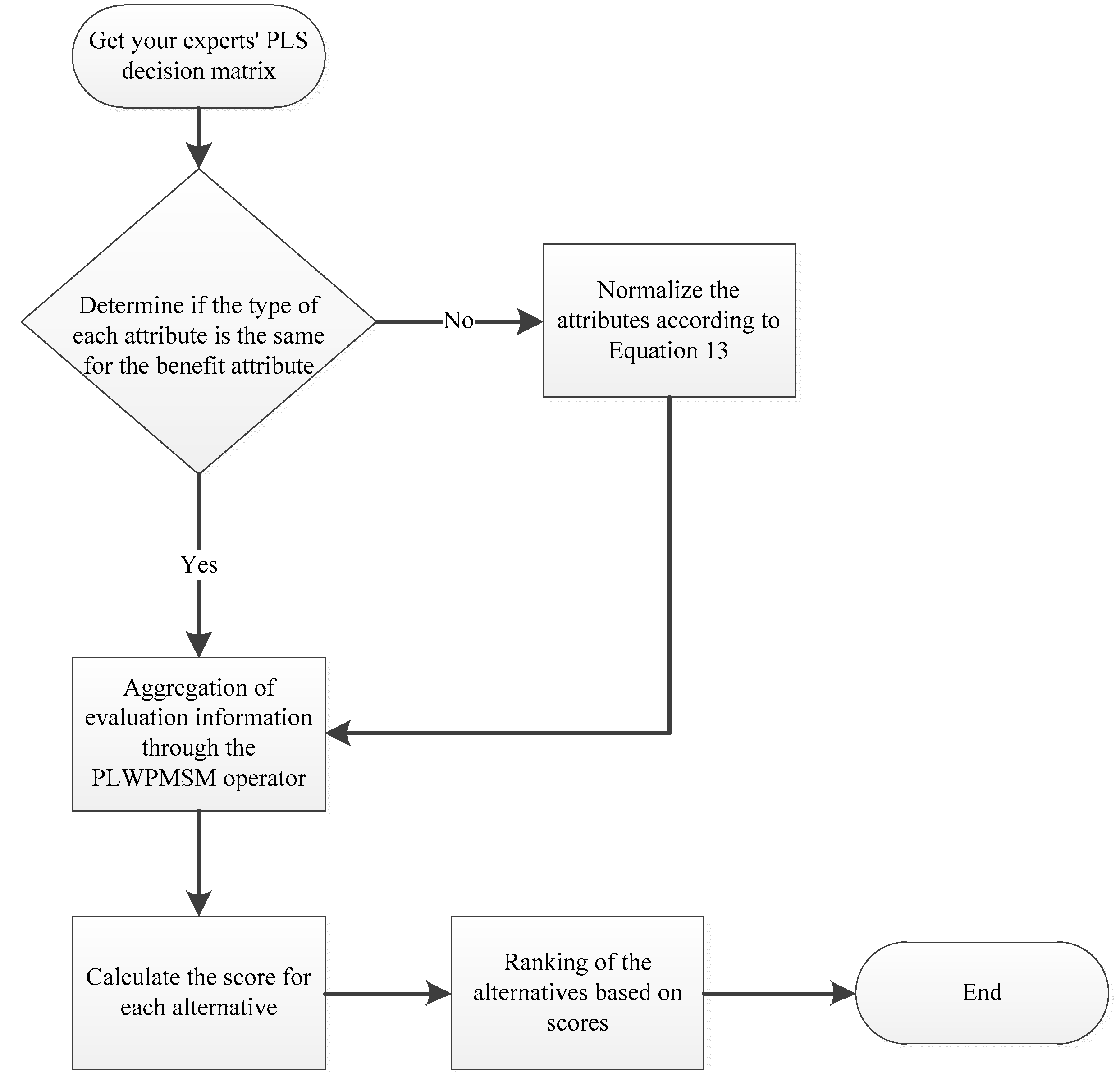
For the above multi-attribute decision problem, the evaluation information is next processed using the WPSPMSM operator as shown in Figure 1 to obtain the best solution, and the main decision steps are as follows:

Step 1: 

Standardize the attribute values.

Step 1 is the normalization of the evaluation matrix. Depending on the characteristics of the attributes, they can be divided into two categories, cost and benefit. To eliminate the influence of different types of attributes, normalize the attributes to a single form of benefit attributes. Convert cost-based attributes to benefit-based attributes via a conversion function $\psi ={\left[Ts{\left(\pi \right)}_{ij}\right]}_{l\times n}$, where:

$$Ts{\left(\pi \right)}_{ij}=\left\{\begin{array}{l}\left\{T{s}_{ij}^{\left(\tau \right)}|\tau =1,2,\dots ,\#Ts{\left(\pi \right)}_{ij}\right\}{ \mathrm{for} \mathrm{benefit} \mathrm{attribute} \mathrm{F}}_j\\ \left\{-T{s}_{ij}^{\left(\tau \right)}|\tau =1,2,\dots ,\#Ts{\left(\pi \right)}_{ij}\right\}{ \mathrm{for} \cos \mathrm{t} \mathrm{attribute} \mathrm{F}}_j\end{array}\right.$$

(14)

Step 2: 

By analyzing the relationship between the attributes, the attributes with mutual relationships are classified into the same category.

Step 3: 

The aggregation operator proposed in this paper is used to calculate the evaluation information after classification in order to obtain the evaluation value of each alternative.

Step 4: 

The best alternative is obtained by ranking the alternatives $Z_i\left(i=1,2,\dots ,l\right)$ according to the score function $\psi \left(T{s}_i\right)$ and the exact function $\overline{\sigma }\left(T{s}_i\right)$.

Step 5: 

End.

4. Case Study and Discussion

4.1. Application in the Evaluation of Green Suppliers

The environmental friendliness and sustainability of manufacturing enterprises are also receiving attention from the government and the public with the introduction of national green and sustainable strategies and technological advances. Many companies have incorporated environmental factors into their supply chains. Suppliers, as an important part of green supply chain management, are evaluated for green production, which is of great environmental and practical importance to the sustainability of a company. A manufacturing company evaluates its suppliers of important components in order to decide on the next stage of supplier management strategy [1]. There are currently four suppliers with which these companies cooperate, and the evaluation attributes are set as follows.

Economic factors ($F_1{}^{\prime }$): Economic factors are the primary factors in the evaluation of suppliers, mainly from the supplier’s product price competitiveness, product localization performance, product logistics costs, and business claims record. Usually, when evaluating suppliers, enterprises evaluate suppliers based on the competitiveness of their product prices among suppliers; the degree of product localization and product logistics costs are the prerequisites for ensuring a stable supply at low cost, and a lower record of business claims ensures a reduction in variable costs.

Green production (${F^{\prime }}_2$): This mainly includes the level of environmental certification, the risk of production processes, pollutant emissions and disposal, and the record of environmental penalties. A high environmental certification level is a prerequisite for the supplier’s environmental proof. Risks are classified according to the processes designed for the parts in the production process, and a more comprehensive evaluation of the supplier can be made based on historical data, such as the supplier’s three waste emissions and environmental records.

Technological innovation (${F^{\prime }}_3$): investment in technological research and development, the level of research and development in environmental technology, and the ability to produce green technology. Investment in R&D is a prerequisite for the technological upgrading of enterprises, and a superior technology level is a prerequisite for long-term and stable cooperation.

Green products (${F^{\prime }}_4$): environmental protection level of components and raw materials, natural resource consumption, and green design. The environmental protection level of components is assessed from the perspective of the design and procurement of the supplier’s component products.

Product quality (${F^{\prime }}_5$): Product quality factors include product defect rates, quality response time, and quality certification systems. Having a higher level of quality certification is a prerequisite for supplier quality assurance. Reduced product defects and rapid quality response time are prerequisites for the continued efficient operation of the supply chain.

Service levels (${F^{\prime }}_6$): financial settlement, daily business, and after-sales service performance. A comprehensive evaluation of the supplier’s service level in terms of financial, operational, and after-sales levels provides a solid foundation for improving efficiency.

Four experts were invited to evaluate four suppliers, with the six attributes’ weights being $w=\left(0.2,0.2,0.2,0.1,0.2,0.1\right)$. According to the correlation between the attributes, the attributes can be divided into two parts, $B_1$$\left\{{F^{\prime }}_1,{F^{\prime }}_5,{F^{\prime }}_6\right\}$ and $B_2$$\left\{{F^{\prime }}_2,{F^{\prime }}_3,{F^{\prime }}_4\right\}$, where $B_1$ is the product value, and $B_2$ is the environmental protection level. Experts’ evaluation information is shown in

Table 1. The evaluation values by PLS.

	${{\mathit{F}}^{\prime }}_1$	${{\mathit{F}}^{\prime }}_2$	${{\mathit{F}}^{\prime }}_3$	${{\mathit{F}}^{\prime }}_4$	${{\mathit{F}}^{\prime }}_5$	${{\mathit{F}}^{\prime }}_6$
${Z^{\prime }}_1$	$\left\{{\mathrm{s}}_2\left(0.8\right)\right\}$	$\left\{{\mathrm{s}}_0\left(0.4\right){,\mathrm{s}}_1\left(0.6\right)\right\}$	$\left\{{\mathrm{s}}_2\left(0.6\right)\right\}$	$\left\{{\mathrm{s}}_0\left(0.7\right)\right\}$	$\left\{{\mathrm{s}}_{-1}\left(0.2\right){,\mathrm{s}}_0\left(0.8\right)\right\}$	$\left\{{\mathrm{s}}_2\left(0.6\right)\right\}$
${Z^{\prime }}_2$	$\left\{{\mathrm{s}}_2\left(0.6\right)\right\}$	$\left\{{\mathrm{s}}_1\left(0.3\right){,\mathrm{s}}_2\left(0.7\right)\right\}$	$\left\{{\mathrm{s}}_{-1}\left(0.8\right)\right\}$	$\left\{{\mathrm{s}}_2\left(1\right)\right\}$	$\left\{{\mathrm{s}}_{-2}\left(0.4\right),{\mathrm{s}}_{-1}\left(0.5\right)\right\}$	$\left\{{\mathrm{s}}_1\left(0.7\right)\right\}$
${Z^{\prime }}_3$	$\left\{{\mathrm{s}}_2\left(0.9\right)\right\}$	$\left\{{\mathrm{s}}_1\left(0.8\right),{\mathrm{s}}_2\left(0.6\right)\right\}$	$\left\{{\mathrm{s}}_2\left(0.6\right)\right\}$	$\left\{{\mathrm{s}}_2\left(0.7\right)\right\}$	$\left\{{\mathrm{s}}_0\left(0.2\right),{\mathrm{s}}_1\left(0.5\right)\right\}$	$\left\{{\mathrm{s}}_2\left(1\right)\right\}$
${Z^{\prime }}_4$	$\left\{{\mathrm{s}}_0\left(0.3\right),{\mathrm{s}}_1\left(0.6\right)\right\}$	$\left\{{\mathrm{s}}_{-2}\left(0.8\right)\right\}$	$\left\{{\mathrm{s}}_1\left(0.7\right)\right\}$	$\left\{{\mathrm{s}}_1\left(0.5\right)\right\}$	$\left\{{\mathrm{s}}_2\left(1\right)\right\}$	$\left\{{\mathrm{s}}_1\left(0.6\right),{\mathrm{s}}_2\left(0.4\right)\right\}$

.

The evaluation information was calculated using the PLWPMSM operator to obtain the ranking of suppliers, which was calculated as follows.

Step 1: 

Normalization of attributes.

As the attributes in our scenario were all revenue attributes, the attribute values did not need to be normalized.

Step 2: 

With the proposed PLWPMSM aggregation operator, the aggregated values for all attributes of each alternative were calculated.

Assume that $m=2$ and ${\kappa }_1={\kappa }_2$.

The description of this calculation is omitted here because the amount of data obtained from the calculation is too large.

Step 3: 

The score of each alternative was calculated according to the formulas $\psi \left(T{s}_1\right)=s_{-1.9643}$, $\psi \left(T{s}_2\right)=s_{-2.1077}$, $\psi \left(T{s}_3\right)=s_{-1.6548}$, and $\psi \left(T{s}_4\right)=s_{-2.0899}$.

Step 4: 

The options were ranked according to Definition A5 in Appendix A and ranked as ${Z^{\prime }}_3\succ {Z^{\prime }}_1\succ {Z^{\prime }}_4\succ {Z^{\prime }}_2$.

Comparing the expected values of the four suppliers according to Definition A4 gave $\psi \left(T{s}_3\right)>\psi \left(T{s}_1\right)>\psi \left(T{s}_2\right)>\psi \left(T{s}_4\right)$, and according to the Definition A5, the ranking of the four suppliers can be obtained as ${Z^{\prime }}_3\succ {Z^{\prime }}_1\succ {Z^{\prime }}_4\succ {Z^{\prime }}_2$.

4.2. The Influence of the Parameters $\kappa$

The effect of the parameter $\kappa$ on the results of the proposed method is discussed next. By assigning different values of parameter $\kappa$, where $\kappa$ = 1, 2, and 3, the sorting results with different $\kappa$ values are shown in

Table 2. Ranking of the alternatives based on the PLPMSM operator for the different alternatives.

The Values of $\mathit{\kappa }$	The Scores of the Alternative	Ranking
${\kappa }_1=1$, ${\kappa }_2=1$	$\psi \left(T{s}_1\right)=s_{0.8607}$, $\psi \left(T{s}_2\right)=s_{0.7389}$, $\psi \left(T{s}_3\right)=s_{1.2756}$, $\psi \left(T{s}_4\right)=s_{0.5791}$	${Z^{\prime }}_3\succ {Z^{\prime }}_1\succ {Z^{\prime }}_4\succ {Z^{\prime }}_2$
${\kappa }_1=1$, ${\kappa }_2=2$	$\psi \left(T{s}_1\right)=s_{-1.9403}$, $\psi \left(T{s}_2\right)=s_{-2.0667}$, $\psi \left(T{s}_3\right)=s_{-1.6364}$, $\psi \left(T{s}_4\right)=s_{-2.0515}$	${Z^{\prime }}_3\succ {Z^{\prime }}_1\succ {Z^{\prime }}_4\succ {Z^{\prime }}_2$
${\kappa }_1=1$, ${\kappa }_2=3$	$\psi \left(T{s}_1\right)=s_{-1.9433}$, $\psi \left(T{s}_2\right)=s_{-2.1096}$, $\psi \left(T{s}_3\right)=s_{-1.6490}$, $\psi \left(T{s}_4\right)=s_{-2.0384}$	${Z^{\prime }}_3\succ {Z^{\prime }}_1\succ {Z^{\prime }}_2\succ {Z^{\prime }}_4$
${\kappa }_1=2$, ${\kappa }_2=1$	$\psi \left(T{s}_1\right)=s_{-1.9749}$, $\psi \left(T{s}_2\right)=s_{-2.0304}$, $\psi \left(T{s}_3\right)=s_{-1.6338}$, $\psi \left(T{s}_4\right)=s_{-2.0598}$	${Z^{\prime }}_3\succ {Z^{\prime }}_1\succ {Z^{\prime }}_2\succ {Z^{\prime }}_4$
${\kappa }_1=2$, ${\kappa }_2=2$	$\psi \left(T{s}_1\right)=s_{-1.9642}$, $\psi \left(T{s}_2\right)=s_{-2.1078}$, $\psi \left(T{s}_3\right)=s_{-1.6548}$, $\psi \left(T{s}_4\right)=s_{-2.0899}$	${Z^{\prime }}_3\succ {Z^{\prime }}_1\succ {Z^{\prime }}_4\succ {Z^{\prime }}_2$
${\kappa }_1=2$, ${\kappa }_2=3$	$\psi \left(T{s}_1\right)=s_{-1.9672}$, $\psi \left(T{s}_2\right)=s_{-2.1512}$, $\psi \left(T{s}_3\right)=s_{-1.6673}$, $\psi \left(T{s}_4\right)=s_{-2.1128}$	${Z^{\prime }}_3\succ {Z^{\prime }}_1\succ {Z^{\prime }}_4\succ {Z^{\prime }}_2$
${\kappa }_1=3$, ${\kappa }_2=1$	$\psi \left(T{s}_1\right)=s_{-1.9754}$, $\psi \left(T{s}_2\right)=s_{-2.0630}$, $\psi \left(T{s}_3\right)=s_{-1.6494}$, $\psi \left(T{s}_4\right)=s_{-2.0909}$	${Z^{\prime }}_3\succ {Z^{\prime }}_1\succ {Z^{\prime }}_2\succ {Z^{\prime }}_4$
${\kappa }_1=3$, ${\kappa }_2=2$	$\psi \left(T{s}_1\right)=s_{-1.9783}$, $\psi \left(T{s}_2\right)=s_{-2.1408}$,.$\psi \left(T{s}_3\right)=s_{-1.66705}$, $\psi \left(T{s}_4\right)=s_{-2.1212}$	${Z^{\prime }}_3\succ {Z^{\prime }}_1\succ {Z^{\prime }}_4\succ {Z^{\prime }}_2$
${\kappa }_1=3$, ${\kappa }_2=3$	$\psi \left(T{s}_1\right)=s_{-1.9813}$, $\psi \left(T{s}_2\right)=s_{-2.1844}$, $\psi \left(T{s}_3\right)=s_{-1.6830}$, $\psi \left(T{s}_4\right)=s_{-2.1442}$	${Z^{\prime }}_3\succ {Z^{\prime }}_1\succ {Z^{\prime }}_4\succ {Z^{\prime }}_2$

.

The following conclusions can be drawn from Table 2.

(1)

When $\kappa =1$, the ranking result of the four firms is: ${Z^{\prime }}_3\succ {Z^{\prime }}_1\succ {Z^{\prime }}_2\succ {Z^{\prime }}_4$; the best alternative is ${Z^{\prime }}_3$.

(2)

When $\kappa =2$ or 3, the ranking result of the four firms is: ${Z^{\prime }}_3\succ {Z^{\prime }}_1\succ {Z^{\prime }}_4\succ {Z^{\prime }}_2$; the best option is likewise ${Z^{\prime }}_3$.

It is obvious that the ranking order may vary with the parameter $\kappa$; however, in this case, the most appropriate choice remained the same. By further analysis, it can be seen that for the same decision information, the expectation value obtained by the MADM method decreased with the increase in the parameter $\kappa$. Moreover, it can also be used to describe the DM’s preferences. Usually, decision makers need to give a suitable value to the parameter $\kappa$ according to their preferences in the current decision. To further explore the effect of the parameter $\kappa$ on the scores and ranking of the alternative firms, different values were assigned to $\kappa$ to each part of ${\kappa }_1=$ 1, 2, 3 and ${\kappa }_2=$ 1, 2, 3. It can be seen from Table 2 that for different values $\kappa$, the scores and ranking results of the four alternative firms differed somewhat, but the best ranking solution for different values were all ${Z^{\prime }}_3$. Moreover, for the same alternative company, the score obtained using the WPLPMSM operator decreased as the value $\kappa$ increased, following the previous theorem. According to the characteristics of the WPLPMSM aggregation operator, the adjustment of the parameters ${\kappa }_{\gamma }$ can reflect the DM’s preference for risk. When the DM is a risk-neutral person, he or she chooses a larger value within the allowed range, and when the DM is a risk-averse person, he or she prefers to choose a smaller value. Management’s attitude to risk should be neutral and take into account the correlation among attributes when making decisions. Therefore, Qin and Liu suggested setting a parameter ${\kappa }_{\gamma }=\left[\underset{\gamma }{\min }\left|B_{\gamma }\right|/2\right]$ to denote the value adopted by the risk-neutral DMs [38], where denotes the conditional number in the partition, and the symbol [] represents the downward integer. When ${\kappa }_{\gamma }>\left[\underset{\gamma }{\min }\left|B_{\gamma }\right|/2\right]$, it represents that the DM is optimistic, that is, risk-neutral, and when ${\kappa }_{\gamma }<\left[\underset{\gamma }{\min }\left|B_{\gamma }\right|/2\right]$, it represents that the DM is pessimistic, that is, risk-averse. In the above example, it can be found that the best option is the third firm, because the DMs are unbiased.

4.3. Comparison and Sensitivity Analysis

In this section, the effectiveness and superiority of the evaluation method are emphasized by comparison with other existing methods, such as the PLWA operator used by Pang and the PLWMSM operator proposed by Liu [22,41].

When comparing with Pang’s approach, it is necessary to establish the prerequisite that all attributes are located in the same partition; the latter assumptions do not take into account the correlation among attributes and the partitioning of attributes. The method of this paper was compared with Pang’s method, as shown in

Table 3. A comparison of the ranking results for different MAGDM methods.

Aggregation Operator	$\mathbf{Expected} \mathbf{Values} \mathit{\psi }\left(\mathit{T}{\mathit{s}}_1\right)$	Ranking
PLWA	$\psi \left(T{s}_1\right)=s_{-2.0066}$$, \psi \left(T{s}_2\right)=s_{-2.19237}$$, \psi \left(T{s}_3\right)=s_{-1.6881}$$, \psi \left(T{s}_4\right)=s_{-2.2024}$	${Z^{\prime }}_3\succ {Z^{\prime }}_1\succ {Z^{\prime }}_2\succ {Z^{\prime }}_4$
PLMSM $(\kappa =2$)	$\psi \left(T{s}_1\right)=s_{-1.9355}$$, \psi \left(T{s}_2\right)=s_{-2.0530}$$, \psi \left(T{s}_3\right)=s_{-1.6348},$$\psi \left(T{s}_4\right)=s_{-2.0740}$	${Z^{\prime }}_3\succ {Z^{\prime }}_1\succ {Z^{\prime }}_2\succ {Z^{\prime }}_4$
Proposed method $(m=1$$, \kappa =1$)	$\psi \left(T{s}_1\right)=s_{1.1354}$$, \psi \left(T{s}_2\right)=s_{1.0112}$$, \psi \left(T{s}_3\right)=s_{1.75364}$$, \psi \left(T{s}_4\right)=s_{0.9367}$	${Z^{\prime }}_3\succ {Z^{\prime }}_1\succ {Z^{\prime }}_2\succ {Z^{\prime }}_4$
Proposed method $(m=2$$, {\kappa }_1={\kappa }_2=1$)	$\psi \left(T{s}_1\right)=s_{0.8607}$$, \psi \left(T{s}_2\right)=s_{0.7389}$$, \psi \left(T{s}_3\right)=s_{1.2756}$$, \psi \left(T{s}_4\right)=s_{0.5791}$	${Z^{\prime }}_3\succ {Z^{\prime }}_1\succ {Z^{\prime }}_2\succ {Z^{\prime }}_4$
Proposed method $(m=2$$, {\kappa }_1={\kappa }_2=2$)	$\psi \left(T{s}_1\right)=s_{-1.9813}$$, \psi \left(T{s}_2\right)=s_{-2.1844}$$, \psi \left(T{s}_3\right)=s_{-1.6830}$$, \psi \left(T{s}_4\right)=s_{-2.1442}$	${Z^{\prime }}_3\succ {Z^{\prime }}_1\succ {Z^{\prime }}_4\succ {Z^{\prime }}_2$
Proposed method $(m=2$$, {\kappa }_1={\kappa }_2=3$)	$\psi \left(T{s}_1\right)=s_{-1.9813}$$, \psi \left(T{s}_2\right)=s_{-2.1844}$$, \psi \left(T{s}_3\right)=s_{-1.6830}$$, \psi \left(T{s}_4\right)=s_{-2.1442}$	${Z^{\prime }}_3\succ {Z^{\prime }}_1\succ {Z^{\prime }}_4\succ {Z^{\prime }}_2$

, where $m=1$ and $\kappa =1$. The results $Z_3{}^{\prime }\prec Z_1{}^{\prime }\prec Z_2{}^{\prime }\prec Z_4{}^{\prime }$ obtained by this method are consistent with Pang’s method. However, the results obtained when the parameter of the proposed method was $m=2$ and $\kappa =2,3$ were different. The PLWA operator does not take into account the correlation between attributes and the classification of attribute classes. For instance, if the correlation among attributes were ignored, then Pang’s method and the method in this paper should yield consistent conclusions. Applying the operator of this paper and Pang’s method to the example separately, it can be found that when $m=1$ and $\kappa =1$, the ranking results of both methods were the same, which is consistent with our analysis of PLWA as a special case of the PLWPMSM operator. However, when $m=2$ and $\kappa =2,3$, our method’s results differed from Pang’s results, because our method reflects the classification of attributes and the correlation of attributes, while the PWLA operator does not reflect the correlation and classification between attributes. The results show that our method can address not only the problem of attribute correlation and attribute classification, but also the case of attribute-free relationship classification. This is because the method in this paper has stronger generality than Pang’s method.

Similar to the method by Pang et al., the method proposed by Liu et al. also does not consider the case of attribute partitioning. Therefore, assuming that there is only one partition of attributes in this example, the proposed method was compared with the method proposed by Liu et al. Table 3 shows the comparison results between the proposed method and Liu et al.’s method. Similar to Pang’s method, the method based on MSM operator does not consider attribute partitioning. Hence, it was supposed that there is no partitioning of the properties in the instance, and the proposed method was then compared with Liu’s method. Table 3 shows the results of the comparison between this paper’s method and Liu’s method.

The MSM operator proposed by Liu only considers the correlation among attributes and does not consider attribute partitioning. In this example, if the parameter is set to $m=1$, the attributes are not partitioned, and only the correlation between the attributes $\kappa =2$ is considered, which should have consistent results with Liu’s method. The two methods were applied separately to this example. When Liu et al.’s method and the proposed PLWPMSM operator are applied to the case, it is known that the two methods yield consistent results for the ranking of alternatives with parameters and $\kappa =2$, which is consistent with the proof above that the MSM operator is a special case of the PLWPMSM operator, indicating the effectiveness of the new method. It can be concluded that when $m=1$, the ranking results obtained by using these two methods separately are the same, which is consistent with the conclusion that the MSM operator is a special case of the PLWPMSM operator, and also shows the effectiveness of the new method. However, in this case, all the attributes were divided into two categories, and it was difficult to accurately capture the correlation between the attributes by using Liu’s approach. Therefore, the approach in this paper has better applicability and handles the problem well, regardless of how attributes are divided.

The method was used in different examples and compared with the original calculation method in order to illustrate the effectiveness and superiority of the method.

Referring to the example of Pang et al. in selecting a hospital to validate our proposed method, there are three alternative hospitals to be evaluated from four criteria (the investment fund of the hospital, the level of information technology of the healthcare professionals, and the original level of information technology of the hospital mainly include the level of hardware and software and the support of the local government) to select the most suitable hospital as a pilot hospital for future smart medical projects [22]. The decision matrix is given in

Table 4. Evaluation Information of Smart Hospital.

	${{\mathit{F}}^{″}}_1$	${{\mathit{F}}^{″}}_2$	${{\mathit{F}}^{″}}_3$	${{\mathit{F}}^{″}}_4$
${Z^{″}}_1$	$\left\{{\mathrm{s}}_3\left(0.4\right),{\mathrm{s}}_4\left(0.6\right)\right\}$	$\left\{s_2\left(0.2\right),s_4\left(0.8\right)\right\}$	$\left\{{\mathrm{s}}_3\left(0.2\right),{\mathrm{s}}_4\left(0.8\right)\right\}$	$\left\{{\mathrm{s}}_3\left(0.4\right),{\mathrm{s}}_5\left(0.6\right)\right\}$
${Z^{″}}_2$	$\left\{{\mathrm{s}}_5\left(0.2\right),{\mathrm{s}}_3\left(0.8\right)\right\}$	$\left\{{\mathrm{s}}_2\left(0.2\right){,\mathrm{s}}_3\left(0.4\right),{\mathrm{s}}_4\left(0.2\right)\right\}$	$\left\{{\mathrm{s}}_1\left(0.2\right){,\mathrm{s}}_2\left(0.4\right),{\mathrm{s}}_3\left(0.2\right)\right\}$	$\left\{{\mathrm{s}}_4\left(0.2\right),{\mathrm{s}}_3\left(0.8\right)\right\}$
${Z^{″}}_3$	$\left\{{\mathrm{s}}_3\left(0.6\right),{\mathrm{s}}_4\left(0.4\right)\right\}$	$\left\{{\mathrm{s}}_3\left(0.6\right),{\mathrm{s}}_4\left(0.2\right)\right\}$	$\left\{{\mathrm{s}}_3\left(0.2\right),{\mathrm{s}}_4\left(0.2\right),{\mathrm{s}}_5\left(0.2\right)\right\}$	$\left\{{\mathrm{s}}_4\left(0.8\right),{\mathrm{s}}_6\left(0.2\right)\right\}$

, and the example is then processed by the MADM method of this paper. The ranking scheme obtained by the method based on the PLWPMSM aggregation operator in this paper was analyzed in comparison with the scheme of the PLWA operator. As shown in

Table 5. Comparison using two methods.

Aggregation Operator	$\mathbf{Expected} \mathbf{Values} \mathit{\psi }\left(\mathit{T}{\mathit{s}}_{\mathit{i}}\right)$	Ranking
PLWA	$\psi \left(T{s}_1\right)=s_{1.26}$$, \psi \left(T{s}_2\right)=s_{0.89}$$, \psi \left(T{s}_2\right)=s_{1.24}$	${Z^{″}}_1\succ {Z^{″}}_3\succ {Z^{″}}_2$
Proposed method $(m=1$$, {\kappa }_1={\kappa }_2=1$)	$\psi \left(T{s}_1\right)=s_{1.26}$$, \psi \left(T{s}_2\right)=s_{0.89}$$, \psi \left(T{s}_3\right)=s_{1.24}$	${Z^{″}}_1\succ {Z^{″}}_3\succ {Z^{″}}_2$
Proposed method $(m=2$$, {\kappa }_1={\kappa }_2=2$)	$\psi \left(T{s}_1\right)=s_{-1.6861}$$, \psi \left(T{s}_2\right)=s_{-2.1893}$$, \psi \left(T{s}_3\right)=s_{-1.6347}$	${Z^{″}}_3\succ {Z^{″}}_1\succ {Z^{″}}_2$

, these properties can be divided into two groups: the hospital investment funds and the support of the local government as the external factors, namely $Q_1=\left\{{F^{″}}_1,{F^{″}}_4\right\}$, and the information level of medical staff and the hospital information level of the original as internal factors, namely $Q_2=\left\{{F^{″}}_2,{F^{″}}_3\right\}$. Table 4 below gives the decision matrix. The MADM method was proposed to deal with an example, the method based on WPLPMSM aggregation operator was also used, and Pang and others were compared based on PLWA operators; then, a solution was obtained, as shown in Table 5.

The attributes in this case were divided into two parts. Each part had two attributes, namely $Q_1=\left\{{F^{″}}_1,{F^{″}}_4\right\}$ and $Q_2=\left\{{F^{″}}_2,{F^{″}}_3\right\}$, so $\kappa$ in each partition could take the value of 1 or 2, and there was a certain relationship between the two attributes, so the result of taking ${\kappa }_1={\kappa }_2=2$ to obtain the sorting result of the scheme was $Z_3{}^{″}\succ Z_1{}^{″}\succ Z_2{}^{″}$, which was different from the sorting scheme obtained by the complementary PLWA operator. This is because our MADM method considers the mutual relations between attributes in the same group, and the MADM PLWA operator method was used, which does not reflect the relationship between the property and the different properties among the difference. A comparison with Pang’s method shows that the PLWPMSM operator has greater generality and advantages.

Referring to the example given by Liu et al., suppose the company has an idle amount of money available for investment. Now, there are four projects to choose from for investment. However, these projects have potential gains as well as risks of loss. Therefore, the company invited relevant experts to evaluate the project from four aspects: $F_1{}^{‴}$ the financial perspective, $F_2{}^{‴}$ customer satisfaction, $F_3{}^{‴}$ internal business process, and $F_4{}^{‴}$ learning and growth, and the evaluation information is shown in

Table 6. Evaluation information of investment projects.

	${{\mathit{F}}^{‴}}_1$	${{\mathit{F}}^{‴}}_2$	${{\mathit{F}}^{‴}}_3$	${{\mathit{F}}^{‴}}_4$
${Z^{‴}}_1$	$\left\{{\mathrm{s}}_2(1)\right\}$	$\left\{{\mathrm{s}}_1\left(0.6\right)\right\}$	$\left\{{\mathrm{s}}_3\left(0.4\right),{\mathrm{s}}_4\left(0.4\right)\right\}$	$\left\{{\mathrm{s}}_3\left(0.8\right)\right\}$
${Z^{‴}}_2$	$\left\{{\mathrm{s}}_2\left(0.8\right)\right\}$	$\left\{{\mathrm{s}}_1\left(0.8\right)\right\}$	$\left\{{\mathrm{s}}_0\left(0.6\right){,\mathrm{s}}_1\left(0.2\right)\right\}$	$\left\{{\mathrm{s}}_2\left(0.6\right)\right\}$
${Z^{‴}}_3$	$\left\{{\mathrm{s}}_1\left(0.4\right)\right\}$	$\left\{{\mathrm{s}}_3\left(0.6\right)\right\}$	$\left\{{\mathrm{s}}_2\left(0.8\right),{\mathrm{s}}_3\left(0.2\right)\right\}$	$\left\{{\mathrm{s}}_0\left(0.5\right)\right\}$
${Z^{‴}}_4$	$\left\{{\mathrm{s}}_1\left(0.8\right)\right\}$	$\left\{{\mathrm{s}}_1\left(0.6\right)\right\}$	$\left\{{\mathrm{s}}_3\left(0.5\right),{\mathrm{s}}_4\left(0.5\right)\right\}$	$\left\{{\mathrm{s}}_2\left(1\right)\right\}$

, to select the best project to maximize profits. These attributes can be divided into two groups: customer satisfaction, internal business processes, and organizational learning and growth, as a related set of attributes, and then financial perspective as a separate set of attributes, i.e., $Q_1=\left\{{F^{‴}}_1\right\}$, $Q_2=\left\{{F^{‴}}_2,{F^{‴}}_3,{F^{‴}}_4\right\}$.

From the obtained

Table 7. Comparison of two methods.

Aggregation Operator	$\mathbf{Expected} \mathbf{Values} \mathit{\psi }\left(\mathit{T}{\mathit{s}}_{\mathit{i}}\right)$	Ranking
HPLAWMM	$\psi \left(T{s}_1\right)=2.09$$, \psi \left(T{s}_2\right)=0.35$$, \psi \left(T{s}_3\right)=0$$, \psi \left(T{s}_4\right)=1.56$	${Z^{‴}}_1\succ {Z^{‴}}_4\succ {Z^{‴}}_2\succ {Z^{‴}}_3$
Proposed method $(m=2$$, {\kappa }_1=1$$, {\kappa }_2=2$)	$\psi \left(T{s}_1\right)=s_{0.7811}$$, \psi \left(T{s}_2\right)=s_{0.6121}$$, \psi \left(T{s}_3\right)=s_{1.1322}$$, \psi \left(T{s}_4\right)=s_{1.1671}$	${Z^{‴}}_4\succ {Z^{‴}}_3\succ {Z^{‴}}_1\succ {Z^{‴}}_2$
Proposed method $(m=2$$, {\kappa }_1=1$$, {\kappa }_2=3$)	$\psi \left(T{s}_1\right)=s_{0.7380}$$, \psi \left(T{s}_2\right)=s_{0.5785}$$, \psi \left(T{s}_3\right)=s_{1.0542}$$, \psi \left(T{s}_4\right)=s_{1.1474}$	${Z^{‴}}_4\succ {Z^{‴}}_3\succ {Z^{‴}}_1\succ {Z^{‴}}_2$

, it can be seen that the MADM method for the PLWPMSM aggregation operator and the MADM for the HPLAWMM operator give extremely different results. $Z_1{}^{‴}$ was identified as the best solution, and $Z_3{}^{‴}$ was identified as the worst solution by the HPLAWMM. The PLWPMSM, however, yielded a ranking scheme of $Z_4{}^{‴}\succ Z_3{}^{‴}\succ Z_1{}^{‴}\succ Z_2{}^{‴}$, where the optimal choice was $Z_4{}^{‴}$ and the poorest choice was $Z_2{}^{‴}$. The improved method classifies attributes into different classes based on the PLWPMSM operator and assumes that the attributes in each class are related to each other, but Liu’s calculation assumes that all attributes are related, which ignores the presence of irrelevant ones in the attributes, so the approach here is more sensible.

The proposed MADM method captures the relationship among attributes and can be classified into several parts, whereas Liu’s MADM method can only represent the relationship between attributes. Furthermore, Pang’s MADM method simply aggregates the evaluation information without taking into account the correlation among attributes in the aggregation process. As the proposed MADM method is able to divide attributes into multiple partitions, it takes into account the correlation among multiple attributes in the same category, as well as the independence of attributes in different categories. Therefore, it has better generality and validity compared to previous methods.

5. Conclusions

As environmental awareness grows, a growing number of manufacturing companies are considering environmental performance and establishing green supplier evaluation systems. In this paper, considering the current actual supplier cooperation model, indicators related to green production are added to the evaluation system of component suppliers. This paper also proposes a MADM method that considers the correlation between attributes by converting qualitative information into computable quantitative information through probabilistic linguistic information to evaluate component suppliers. The findings of this study are divided into the following main aspects.

From the perspective of green supplier evaluation, green production-related indicators are added to the component supplier evaluation system, ensuring the quality, timely delivery, and environmental protection of components in the production process, thereby improving the environmental performance and sustainable competitiveness of the enterprise. Meanwhile, this paper provides decision support for enterprises to give management to their cooperative suppliers to create a more environmentally friendly, stable, and efficient supply chain. It can also provide a reference for future studies to consider supplier evaluation issues for green production.

From the perspective of decision-making methods, a decision-making method based on probabilistic linguistic information is proposed to solve the problem that attributes can be divided into different groups according to their interrelationships, and attributes in the same group are related to each other, while attributes in different groups are not related to each other. In addition, the proposed PLWPMSM operator can be converted to other commonly used operators by adjusting the parameters, is highly flexible and general, and provides a general solution to many realistic decision-making problems.

This article also has some limitations, in that some of the evaluation information in the study relies on expert opinions, which may have a partial cognitive bias; on the other hand, only the evaluation of cooperative suppliers was focused on in the study, and the dynamic adjustment of subsequent orders was not taken into account.

In future research, green production indicators in terms of carbon emission reduction can be quantified, and supplier evaluation and order share allocation can be combined for dynamic decision making. In addition, it can be considered that the method proposed in this paper could also be applied to other MADM problems, such as online based product recommendation, as well as charging pile site planning.

References

- Zheng, M.; Li, Y.; Su, Z.; Fan, Y.V.; Jiang, P.; Varbanov, P.S.; Klemeš, J.J. Supplier Evaluation and Management Considering Greener Production in Manufacturing Industry. J. Clean. Prod. 2022, 342, 130964. [Google Scholar] [CrossRef]
- Terpend, R.; Krause, D.R. Competition or Cooperation? Promoting Supplier Performance with Incentives Under Varying Conditions of Dependence. J. Supply Chain Manag. 2015, 51, 29–53. [Google Scholar] [CrossRef] [Green Version]
- Lager, T.; Frishammar, J. Equipment Supplier/User Collaboration in the Process Industries: In Search of Enhanced Operating Performance. J. Manuf. Technol. Manag. 2010, 21, 698–720. [Google Scholar] [CrossRef]
- Zhong, Y.; Gao, H.; Guo, X.; Qin, Y.; Huang, M.; Luo, X. Dombi Power Partitioned Heronian Mean Operators of Q-Rung Orthopair Fuzzy Numbers for Multiple Attribute Group Decision Making. PLoS ONE 2019, 14, e0222007. [Google Scholar] [CrossRef] [PubMed] [Green Version]
- Xu, Z.; Zhang, S. An Overview on the Applications of the Hesitant Fuzzy Sets in Group Decision-Making: Theory, Support and Methods. Front. Eng. Manag. 2019, 6, 163–182. [Google Scholar] [CrossRef]
- Liu, A.; Liu, T.; Ji, X.; Lu, H.; Li, F. The Evaluation Method of Low-Carbon Scenic Spots by Combining IBWM with B-DST and VIKOR in Fuzzy Environment. Int. J. Environ. Res. Public Health 2019, 17, 89. [Google Scholar] [CrossRef] [Green Version]
- Hao, X.; Li, M.; Chen, Y. China’s Overcapacity Industry Evaluation Based on TOPSIS Grey Relational Projection Method with Mixed Attributes. Grey Syst. Theory Appl. 2020, 11, 288–308. [Google Scholar] [CrossRef]
- Wu, J.; Sun, J.; Liang, L. Methods and Applications of DEA Cross-Efficiency: Review and Future Perspectives. Front. Eng. Manag. 2021, 8, 199–211. [Google Scholar] [CrossRef]
- Chang, T.-W.; Pai, C.-J.; Lo, H.-W.; Hu, S.-K. A Hybrid Decision-Making Model for Sustainable Supplier Evaluation in Electronics Manufacturing. Comput. Ind. Eng. 2021, 156, 107283. [Google Scholar] [CrossRef]
- Yager, R.R. The Power Average Operator. IEEE Trans. Syst. Man Cybern. A 2001, 31, 724–731. [Google Scholar] [CrossRef]
- Dejian Yu Interval-Valued Intuitionistic Fuzzy Heronian Mean Operators and Their Application in Multi-Criteria Decision Making. Afr. J. Bus. Manag. 2012, 6, 4158–4168. [CrossRef]
- Xu, Z.; Yager, R.R. Intuitionistic Fuzzy Bonferroni Means. IEEE Trans. Syst. Man Cybern. B 2011, 41, 568–578. [Google Scholar] [CrossRef]
- Yager, R.R. On Generalized Bonferroni Mean Operators for Multi-Criteria Aggregation. Int. J. Approx. Reason. 2009, 50, 1279–1286. [Google Scholar] [CrossRef] [Green Version]
- Yang, W.; Pang, Y. New Q-Rung Orthopair Fuzzy Partitioned Bonferroni Mean Operators and Their Application in Multiple Attribute Decision Making: YANGY and PANG. Int. J. Intell. Syst. 2019, 34, 439–476. [Google Scholar] [CrossRef]
- Liu, P.; Chen, S.-M.; Wang, Y. Multiattribute Group Decision Making Based on Intuitionistic Fuzzy Partitioned Maclaurin Symmetric Mean Operators. Inf. Sci. 2020, 512, 830–854. [Google Scholar] [CrossRef]
- Bai, K.; Zhu, X.; Wang, J.; Zhang, R. Some Partitioned Maclaurin Symmetric Mean Based on Q-Rung Orthopair Fuzzy Information for Dealing with Multi-Attribute Group Decision Making. Symmetry 2018, 10, 383. [Google Scholar] [CrossRef] [Green Version]
- Dickson, G.W. An Analysis Of Vendor Selection Systems And Decisions. J. Purch. 1966, 2, 5–17. [Google Scholar] [CrossRef]
- Lin, T.-X.; Wang, X.; Wu, Z.; Chang, C.-C. Application of Fuzzy Analytical Network Process and VIKOR Model in Foreign Trade Supplier Selection. Mob. Inf. Syst. 2021, 2021, 7508673. [Google Scholar] [CrossRef]
- Finkbeiner, M.; Inaba, A.; Tan, R.; Christiansen, K.; Klüppel, H.-J. The New International Standards for Life Cycle Assessment: ISO 14040 and ISO 14044. Int. J. Life Cycle Assess. 2006, 11, 80–85. [Google Scholar] [CrossRef]
- Tseng, M.-L.; Chiu, A.S.F. Evaluating Firm’s Green Supply Chain Management in Linguistic Preferences. J. Clean. Prod. 2013, 40, 22–31. [Google Scholar] [CrossRef]
- Pech, M.; Vaněček, D. Supplier Performance Management in Context of Size and Sector Characteristics of Enterprises. QIP J. 2020, 24, 88. [Google Scholar] [CrossRef] [Green Version]
- Pang, Q.; Wang, H.; Xu, Z. Probabilistic Linguistic Term Sets in Multi-Attribute Group Decision Making. Inf. Sci. 2016, 369, 128–143. [Google Scholar] [CrossRef]
- Gou, X.; Xu, Z. Novel Basic Operational Laws for Linguistic Terms, Hesitant Fuzzy Linguistic Term Sets and Probabilistic Linguistic Term Sets. Inf. Sci. 2016, 372, 407–427. [Google Scholar] [CrossRef]
- Zhang, Y.; Xu, Z.; Wang, H.; Liao, H. Consistency-Based Risk Assessment with Probabilistic Linguistic Preference Relation. Appl. Soft Comput. 2016, 49, 817–833. [Google Scholar] [CrossRef]
- Wang, X.; Wang, J.; Zhang, H. Distance-based Multicriteria Group Decision-making Approach with Probabilistic Linguistic Term Sets. Expert Syst. 2019, 36, e12352. [Google Scholar] [CrossRef]
- Lin, M.; Chen, Z.; Liao, H.; Xu, Z. ELECTRE II Method to Deal with Probabilistic Linguistic Term Sets and Its Application to Edge Computing. Nonlinear Dyn. 2019, 96, 2125–2143. [Google Scholar] [CrossRef]
- Pan, L.; Ren, P.; Xu, Z. Therapeutic Schedule Evaluation for Brain-Metastasized Non-Small Cell Lung Cancer with A Probabilistic Linguistic ELECTRE II Method. Int. J. Environ. Res. Public Health 2018, 15, 1799. [Google Scholar] [CrossRef] [Green Version]
- Bai, C.; Zhang, R.; Qian, L.; Wu, Y. Comparisons of Probabilistic Linguistic Term Sets for Multi-Criteria Decision Making. Knowl.-Based Syst. 2017, 119, 284–291. [Google Scholar] [CrossRef]
- Liu, P.; Li, Y. The PROMTHEE II Method Based on Probabilistic Linguistic Information and Their Application to Decision Making. Informatica 2018, 29, 303–320. [Google Scholar] [CrossRef] [Green Version]
- Zhang, X.; Xing, X. Probabilistic Linguistic VIKOR Method to Evaluate Green Supply Chain Initiatives. Sustainability 2017, 9, 1231. [Google Scholar] [CrossRef]
- Wu, X.; Liao, H. An Approach to Quality Function Deployment Based on Probabilistic Linguistic Term Sets and ORESTE Method for Multi-Expert Multi-Criteria Decision Making. Inf. Fusion 2018, 43, 13–26. [Google Scholar] [CrossRef]
- Mao, X.-B.; Wu, M.; Dong, J.-Y.; Wan, S.-P.; Jin, Z. A New Method for Probabilistic Linguistic Multi-Attribute Group Decision Making: Application to the Selection of Financial Technologies. Appl. Soft Comput. 2019, 77, 155–175. [Google Scholar] [CrossRef]
- Liu, P.; You, X. Linguistic Neutrosophic Partitioned Maclaurin Symmetric Mean Operators Based on Clustering Algorithm and Their Application to Multi-Criteria Group Decision-Making. Artif. Intell. Rev. 2020, 53, 2131–2170. [Google Scholar] [CrossRef]
- Wu, X.; Liao, H.; Xu, Z.; Hafezalkotob, A.; Herrera, F. Probabilistic Linguistic MULTIMOORA: A Multicriteria Decision Making Method Based on the Probabilistic Linguistic Expectation Function and the Improved Borda Rule. IEEE Trans. Fuzzy Syst. 2018, 26, 3688–3702. [Google Scholar] [CrossRef]
- Kobina, A.; Liang, D.; He, X. Probabilistic Linguistic Power Aggregation Operators for Multi-Criteria Group Decision Making. Symmetry 2017, 9, 320. [Google Scholar] [CrossRef] [Green Version]
- Liang, D.; Kobina, A.; Quan, W. Grey Relational Analysis Method for Probabilistic Linguistic Multi-Criteria Group Decision-Making Based on Geometric Bonferroni Mean. Int. J. Fuzzy Syst. 2018, 20, 2234–2244. [Google Scholar] [CrossRef]
- Feng, X.; Zhang, Q.; Jin, L. Aggregation of Pragmatic Operators to Support Probabilistic Linguistic Multi-Criteria Group Decision-Making Problems. Soft Comput. 2020, 24, 7735–7755. [Google Scholar] [CrossRef]
- Qin, J.; Liu, X. An Approach to Intuitionistic Fuzzy Multiple Attribute Decision Making Based on Maclaurin Symmetric Mean Operators. J. Intell. Fuzzy Syst. 2014, 27, 2177–2190. [Google Scholar] [CrossRef]
- Liu, P.; Li, Y. Multi-Attribute Decision Making Method Based on Generalized Maclaurin Symmetric Mean Aggregation Operators for Probabilistic Linguistic Information. Comput. Ind. Eng. 2019, 131, 282–294. [Google Scholar] [CrossRef]
- Dutta, B.; Guha, D. Partitioned Bonferroni Mean Based on Linguistic 2-Tuple for Dealing with Multi-Attribute Group Decision Making. Appl. Soft Comput. 2015, 37, 166–179. [Google Scholar] [CrossRef]
- Liu, P.; Li, Y. A Novel Decision-Making Method Based on Probabilistic Linguistic Information. Cogn. Comput. 2019, 11, 735–747. [Google Scholar] [CrossRef]
Figure 1.
Decision diagram of the proposed method.