Exploring the Complementarity of Offshore Wind Sites to Reduce the Seasonal Variability of Generation

Abstract

Wind energy is a powerful resource contributing to the decarbonization of the electric grid. However, wind power penetration introduces uncertainty about the availability of wind energy. This article addresses the complementarity of remote offshore wind sites in Brazil, demonstrating that strategic distribution of wind farms can significantly reduce the seasonality and the risk of periods without generation and reduce dependence on fossil sources. Field observations, atmospheric reanalysis, and simplified optimization methods are combined to demonstrate generation improvement considering regions under environmental licensing and areas not yet considered for offshore development. Aggregated power results demonstrate that with the relocation of wind turbines, a 68% reduction of the grid seasonal variability is possible, with a penalty of only 9% of the generated energy. This is accomplished through optimization and the inclusion of the northern region, which presents negative correlations with all other stations. More specifically, the north and northeast of Brazil have large seasonal amplitudes. However, out-of-phase wind regimes with a strong negative correlation (R < −0.6) and high-capacity factors ($CF$) during the peak seasons occur in Jan-Feb-Mar in the north ($CF$ > 0.5) and in Aug-Sep-Oct in the northeast ($CF$ > 0.7). These complementary regimes allow for the introduction of the concept of Reserve Wind Power (RWP) plants, wind farms that can be viewed as “reserve sources” for energy security. These can replace the contracts of thermal reserve plants, with resulting economic and environmental advantages. Our analysis suggests that RWP plants can be 20 to 32% cheaper than thermal reserves in the current market.

1. Introduction

Wind energy is one of the most abundant renewable resources for exploration [1], with a geophysical potential larger than 400 TW for the present technology [2]. The current worldwide installed capacity is 743 GW, of which 35 GW is from offshore wind [3]. It is expected that with technology improvements and more competitive prices, 469 GW of new capacity will be added by 2025 [4,5]. As wind power continues to increase its contribution, new challenges are facing power system operators [6]. Problems such as extra costs for systems security [7], voltage and frequency stability, active power control and frequency regulation, reactive power control, and voltage regulation [8] are becoming increasingly complex to handle [9].

In Brazil, the current total electrical installed capacity is 182 GW, with a significant (83%) contribution from renewables. Hydropower provides 60%, followed by 11.7% from wind, 8.7% from biomass, and 2.6% from solar. Intermittent sources already impact the Brazilian grid operation, typically requiring compensation with the dispatch of hydro- and thermoelectric plants by the National System Operator (ONS) [10].

There are no offshore wind farms in Brazil yet, and all present wind turbines are installed over continental areas. The country’s technical offshore resource, however, is quite large, at nearly 1.3 TW for turbine foundations up to 100 m in depth [11,12].

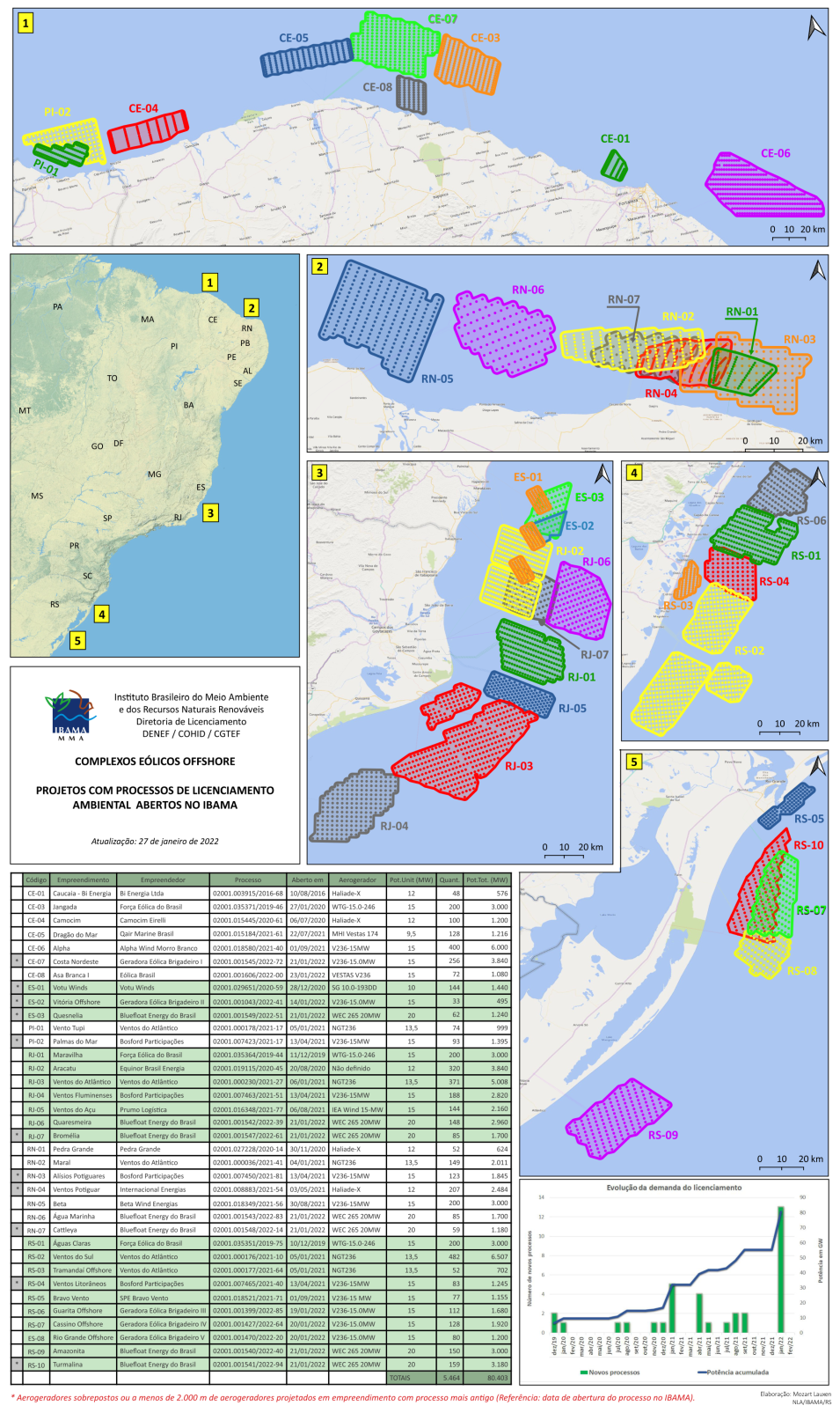
At the time of this writing, nearly 81 GW of offshore wind farms is under environmental licensing at the Brazilian Institute of the Environment and Renewable Natural Resources (IBAMA) (Figure A1). As hydro resources have environmental restrictions for expansion, the expected growth from wind will probably require an increase in thermal plants to balance power and complement ancillary services.

The large-scale exploration of offshore resources requires planning and improvement of the wind systems at different levels of optimization [13]. At the primary level (macro-scale), optimization is concerned with the allocation of wind farms over large geographic distances. General atmospheric circulation, seasonal to interannual variability, weather regimes, and regional complementarity might be considered. Prior studies have relied on onshore stations, meteorological buoys, and ocean towers; combined with turbine power curves, these sources have been used in the simulation of power grids [14,15,16]. More recently, atmospheric reanalysis has provided wind speeds at the turbines’ hub height. Olauson et al. (2018) employed ERA5 and MERRA-2 reanalysis while studying the aggregated wind power of five different countries and the generation of individual wind turbines in Sweden [17]. Berger et al. (2022) proposed an optimization method for wind farm siting in Europe based on reanalysis data [18]. Radu et al. (2022) assessed the impact of offshore wind farms on the design of the European Power System in order to maximize the aggregate power output and its spatiotemporal complementarity [19]. Cazzarro et al.(2022) developed a multi-scale optimization approach that employs ERA5 atmospheric reanalysis [13].

At the secondary level (meso-scale), optimization typically focuses on the optimal shape and positioning of the wind farm relative to the details of the wind fields, wakes from other farms, bathymetry, areas of exclusion, and costs of installation [13]. Pryor et al. (2022) investigated wakes in and between vast offshore arrays off the U.S. east coast using the WRF (Weather Research and Forecasting) model [20].

The third level (micro-scale) of optimization emphasizes the exact positioning (micro-sitting) of turbines within the farm, including technical aspects, wakes of individual turbines, and the performance of the wind park as a whole. Shakoor et al. (2016) developed an optimization method based on the wakes of turbines and the shape of wind farms [21]. Barthelmie et al. (2009) employed Computational Fluid Dynamics (CFD) to model the wakes of the Horns Rev offshore wind farm [22].

While the first optimization level can be performed with tall meteorological towers or products derived from atmospheric reanalysis, the secondary and tertiary optimization levels usually employ high-performance computational methods. Meso-scale studies, in particular, employ numerical weather prediction models and grid nesting for spatial refinement of the winds, which are particularly important in continental regions or near coastal areas with complex topography [23,24]. Atmospheric reanalysis demonstrates good performance compared to offshore observations [25,26]. Reanalysis can demonstrate similar or superior performance compared to meso-scale models for offshore applications in regions far from topographical influences [27,28].

This article addresses the first (macro-scale) optimization level and investigates the aggregate performance of future hypothetical offshore wind farms in Brazil. ERA5 global atmospheric reanalysis, produced by the European Center for Medium-Range Weather Forecasts (ECMWF), is used as a primary source of information [29,30]. ERA5 provides winds at 100 m height with a spatial resolution of 31 km, a temporal resolution of 1 h, and excellent temporal coverage, which is adequate for this type of study. Although ERA5 has been previously validated with towers [31], LIDAR wind profilers [25], and different locations worldwide [26], here, we compare this product to meteorological buoys and hub height winds measured in the oceanic and coastal locations of Brazil.

In this study, ERA5 stations are analyzed for a period of 30 years (1990–2020) to characterize planned offshore wind farms’ seasonality and regional correlation. A modern turbine power curve is employed for the simulation of wind power generation. Wind turbines are distributed among planned sites and other locations not previously considered for offshore exploration. A genetic algorithm (GA) is developed and used to optimize the power grid. It is shown that a specially designed grid can minimize the amplitude of seasonal fluctuations while maximizing the total (aggregate) power generation.

Our results from this grid optimization introduce the concept of Reserve Wind Power (RWP), in analogy with the use of reserve thermal power plants. Offshore sites out of the schedule for deployment (due to low yearly capacity factors) demonstrate high yields during critical periods when other wind farms provide low output. During these periods, the National System Operator (ONS) typically complements the demand with thermal power. RWP represents an emerging alternative to replace this generation, contributing to lower costs and reducing emissions of greenhouse gases (GHG). RWPs can provide energy at lower prices than typical reserve thermal plants.

The rest of this article is organized into three remaining parts: Section 2 describes the databases used for validation and implementation of the methodology, the tools used to prove data quality, and the description and formulation of the problem; Section 3 presents the results along with the devices and parameters used to apply the method; finally, in Section 4, final considerations are made regarding the contributions of this work.

2. Methodology

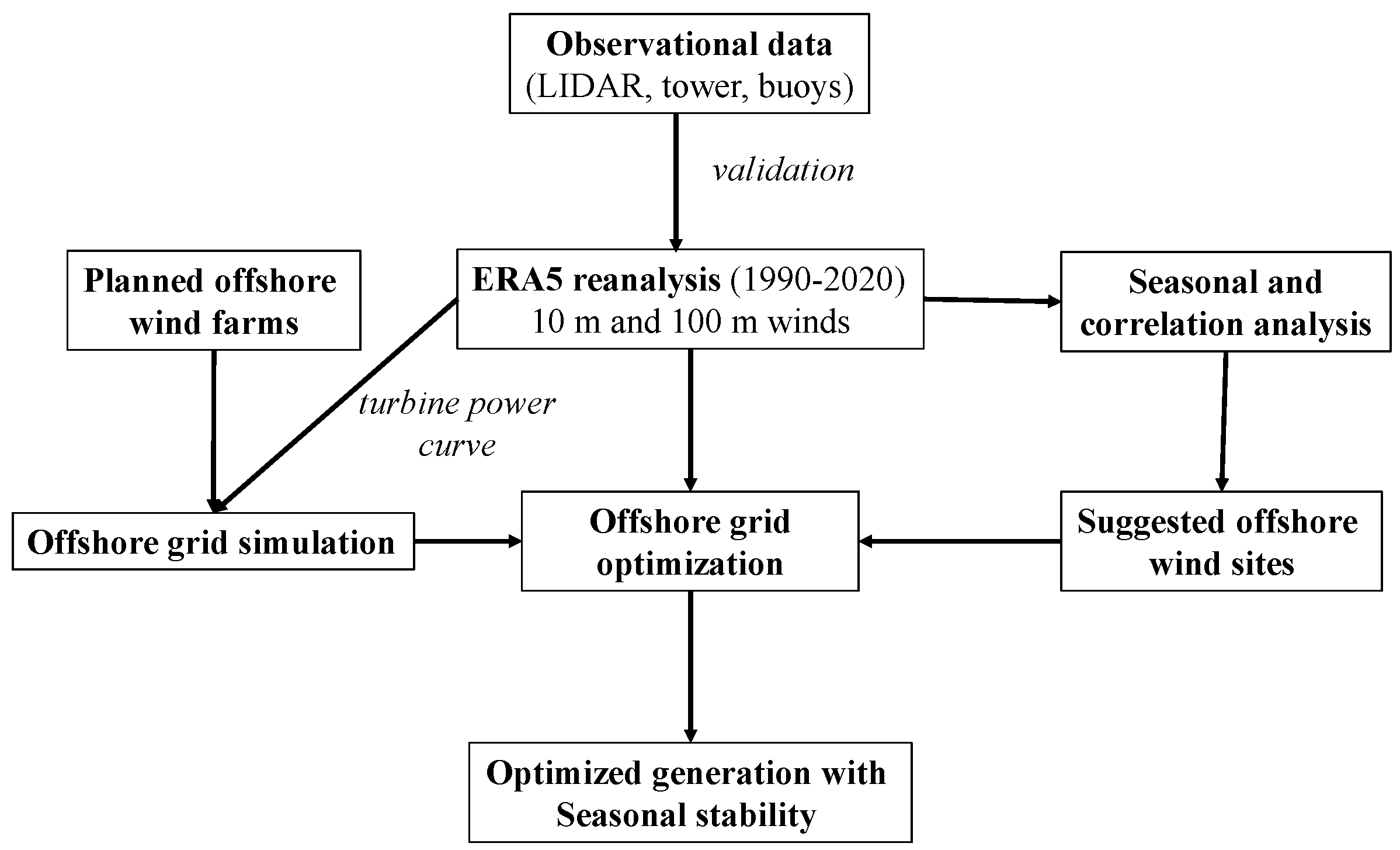
The overall methodology is summarized in Figure 1. First, we describe the observational stations selected for comparison with ERA5 atmospheric reanalysis. Second, the ERA5 reanalysis characteristics are presented, along with the methods used for validation. Third, a description of the 36 offshore wind farms under environmental licensing is presented. These farms are reduced to main offshore locations or wind farm clusters in this study. Selected stations are analyzed for their monthly variability, seasonal signal amplitude, and correlation. Fourth, a multi-objective optimization problem based on a GA is developed for the simulation of different scenarios of wind turbine distributions. The method maximizes the aggregated power while minimizing the seasonal fluctuation.

2.1. Observational Data

The study area comprises the entire Brazilian shelf, which extends over 7000 km from its northern limit at Amapá (4.5${}^{\circ }$ N) to the Rio Grande do Sul (33.7${}^{\circ }$ S) (Figure 2). The observational network over this region is sparse, composed of a few meteorological buoys. Wind information at the height of wind turbines, 100 m above sea level, is rare.

Winds from different sources were combined to validate the ERA5 product. The selected dataset is composed of three meteorological buoys of the Brazilian Navy, an ocean meteorological tower from Petrobrás, a coastal meteorological tower from Alcântara Launch Center (CLA), and two coastal LIDAR stations in the states of Santa Catarina (SC) and Maranhão (MA) (Figure 2).

The meteorological buoys are part of the PNBOIA program carried out by the Brazilian Navy (https://www.marinha.mil.br/chm/dados-do-goos-brasil/pnboia-mapa, accessed on 22 February 2022). Measurements from three buoys for the period between January 2009 and December 2019 were selected for analysis. Their location is indicated in Figure 2 by the yellow bullets. The buoys were designed by Axys Technologies Inc. for offshore measurements and have a diameter of 3.4 m. A meteorological station with two anemometers installed at 3.7 and 4.7 m above the ocean surface records surface wind speeds. Data coverage for the three buoys was $51.89\%$ in Santa Catarina (BUOY-SC), $44.01\%$ in Santos (BUOY-SP), and $59.76\%$ in Rio Grande do Sul (BUOY-RS).

A meteorological tower from Petrobrás (TOWER-PETRO) in the Santos Basin was used as well (Figure 2). We used measurements over 90 days from the winter of 1998 with an hourly time resolution for winds at the reference height of 78 m [32].

A LIDAR (Light Detection and Ranging) station installed over a coastal pier in southern Santa Catarina (LIDAR-SC) was selected. The LIDAR model is a Zephir 300, and the measurement period covered 20 December 2016 to 19 October 2020. Wind records refer to 10 min averages at 110 m above the mean sea level. Data were reduced to hourly averages; a description of the dataset is available in [33,34].

An anemometric tower located in the state of Maranhão at the CLA, Brazilian Air Force (TOWER-MA) provided winds at 72 m above ground level. Data were recorded by an RM Young model 86000 anemometer. The CLA tower is located 300 m from an ocean cliff of 40 m height, making the reference height 112 m above the mean sea level. The measurement period was between April 2017 and December 2019 at 10 min resolution with $24.44\%$ data coverage. For ERA5 comparisons, the data were reduced to hourly time series. This dataset was previously described in [35,36,37,38].

A second LIDAR station, located in the city of Barreirinhas on the east coast of Maranhão state (LIDAR-MA), was used for ERA5 comparisons as well. This LIDAR is a WindCube V2 from Leosphere, providing winds at 100 m covering the months of September to October 2021 with 10 min time resolution. As with the other datasets, the time series was reduced to hourly averages for comparison with ERA5 (Figure 2).

2.2. ERA5 Atmospheric Reanalysis

Reanalysis combines the use of atmospheric forecasting models and sophisticated data assimilating systems in order to provide consistent gap-free maps of essential climate variables [17,30]. ERA5 is the fifth generation of global atmospheric reanalysis generated by the ECMWF [29,30]. This product is based on the Integrated Forecasting System (IFS) Cy41r2, which includes a land surface and an ocean wave model.

ERA5 data assimilation is built on a hybrid incremental four-dimensional (4D-Var) variational system with a 12-h window [39]. The 4D-Var uses observations from over 200 satellites or types of conventional data, extracting information from in situ observations of 10 m winds over the sea, 2 m humidity over land, and pressure over both land and sea. Ocean wind observations include moored meteorological buoys, ships, and satellite platforms. Upper-air observations of wind, temperature, and humidity are obtained from radiosonde, dropsonde, wind profilers, aircraft measurements, and satellites, e.g., atmospheric motion vectors. As the number of assimilated observations has grown substantially over the years, the reliability of ERA5 continues to improve over time [30].

ERA5 presents significant improvements in spatial and temporal resolution compared to ERA-interim, the previous ECMWF reanalysis product [29]. Horizontal grid resolution was changed from 79 km to 31 km, and the number of vertical levels was increased from 60 to 137 levels. The model output frequency was changed from 6 h to 1 h. ERA5 covers 1950 to the present. All these modifications have allowed for better spatial and temporal representation of wind fields at both surface level and at 100 m height [29,30,40].

ERA5 has been compared to other reanalysis products and validated against different sets of observations, including those from meteorological buoys, towers, LIDAR wind profilers, and power generation series, e.g., [17,25,26,31].

Olauson et al. (2018) demonstrated better performance with ERA5 than with MERRA-2 reanalysis (Modern-Era Retrospective Analysis for Research and Applications (MERRA-2) [41]) while studying aggregated wind power data from five different countries and generation from individual wind turbines in Sweden [17]. Correlations were higher, and mean absolute and root mean square errors were 20% lower on average, while the distributions and changes in hourly data were more similar to observations. Ramon et al. (2019a) [31] assessed the performance of five reanalysis datasets, namely, ERA5, ERA-Interim, MERRA-2, JRA55 (Japanese 55-year Reanalysis [42]), and R1 (National Centers for Environmental Prediction (NCEP)/National Center for Atmospheric Research (NCAR) Reanalysis 1) [43]), using a global database of 77 tall towers [44]. ERA5 demonstrated the best correlations and standard deviations. Tavares et al. (2020a) compared three atmospheric reanalysis datasets with five meteorological buoys off Brazil [45]. In general, they found the best performance for ERA5, followed by CFSv2 (NCEP Climate Forecast System [46]) and MERRA-2.

Gualtieri (2022) [26] analyzed the uncertainties of six regional and nine global reanalysis datasets, including ERA5 (Regional reanalysis: NARR, COSMO-REA6, COSMO-REA2, HARMONIEv1, UM, MÉRA; global reanalysis: ERA5, R1, R2, ERA40, ERA-Interim, CFSR, MERRA, CFSv2, MERRA-2), with their results reported in Table 1 of [26]. The results of 322 worldwide stations were analyzed regarding their location (offshore, coastal, inland, and mountainous) and height above the ground (10–300 m). Gualtieri (2022) concluded that global reanalysis data, particularly ERA5, are sufficiently reliable for both offshore and flat onshore locations. The best scores were achieved at offshore sites, with wind speeds being slightly underestimated (median bias = 0.10 m $s^{-1}$) and time variation reproduced well (median correlation R = 0.89).

The application of reanalysis products has evolved for studies in the field of energy, and different studies have employed ERA5 as a primary source of information for wind farm simulations [13,18,19,47,48]. We selected a 30-year period of ERA5 data (1990–2020) from specific locations to characterize Brazilian winds for wind farm simulation.

2.3. ERA5 Validation

The observational data used for comparison were derived from three buoys, two tall towers, and two LIDARs, as described in Section 2.1. Observed wind speeds were paired with ERA5 information derived from the closest offshore grid points. ERA5 winds were selected only for paired valid information on the observational time series. Gaps were not interpolated.

As ERA5 winds are available for 10 and 100 m heights, it was necessary to adjust the observations to match the height of the ERA5 product. Buoy data were extrapolated to a height of 10 m, and tower data were adjusted to 100 m. The velocity at level z can be computed as specified by Equation (1):

$$V=V_r\frac{ln(z/z_0)}{ln(z_r/z_0)}.$$

(1)

where $z_r$ represents the reference height of measurements, z is the desired height (10 m for buoys, 100 m for towers and LIDAR), and the roughness coefficient is $z_o=0.2$ mm. Although the surface roughness of water is not constant and depends on the wavefield, which in turn depends on the wind speed, fetch, etc., the assumption of a constant sea surface roughness is used in applications because of its simplicity (e.g., Lange et al., 2004) [49].

2.4. Planned Offshore Wind Farms

With 1.3 TW of energy potential, Brazil has become a center for offshore wind. A relevant mark for the energy sector was the elaboration of workshops by the Energy Research Enterprise (EPE), linked to the Ministry of Energy, and by the IBAMA, linked to the Ministry of the Environment (MMA).

Developing plans and guidelines for the environmental licensing process have fostered different proposals for offshore wind projects. The first proposal was submitted to IBAMA in August 2016 for Ceará state (CE), with a total installed capacity of 576 MW (Figure A1). In January 2022, nearly 80 GW were in the environmental licensing phase at IBAMA [50]. The largest wind farm plans are for 5 GW of installed capacity on the Rio de Janeiro (RJ) coastline (Figure A1).

Planned offshore wind farms are clustered along the coast of Ceará, Rio Grande do Norte, Espírito Santo and Rio de Janeiro, and Rio Grande do Sul in a total of 36 projects. As can be seen from the regional maps of Figure A1, several states are already experience spatial conflicts as turbine locations overlap between the proposed farms (see PI, RN, RJ, and RS).

The purpose of this work is not to evaluate the details of the future performance of individual wind farms by taking into consideration turbine wake effects or detailed specifications of turbines. Instead, our goal is to evaluate the overall performance of these planned wind clusters by modeling their power generation using the ERA5 historical dataset.

In order to simplify this analysis, wind observations from ERA5 are sampled for the center of these regional clusters of wind farm development, as indicated by the numbers on the larger map in Figure A1. This grouping considers that wind farms are located relatively close together and have similar seasonal characteristics. This is supported by a previous analysis that used Ward’s agglomerative hierarchical method to identify regional similarities for stations along the coast (see Figure 9 in Silva et al., 2016 [11]).

Six wind time series were extracted from ERA5 as a representation of 100 m winds to evaluate the performance of these planned wind farms. The selected locations are indicated in Figure 2 by magenta squares, identified as Piauí (PI), Ceará (CE), Rio Grande do Norte (RN), Rio de Janeiro (RJ) and Rio Grande do Sul (RS-N and RS-S). In addition, three new sites are suggested in this work to improve aggregated generation. These suggested wind farms, identified by magenta squares in Figure 2, are AP (Amapá), MA (Maranhão), and SC (Santa Catarina). The stations’ coordinates are listed in Table 1.

To simplify our analysis, we selected a Vestas V164 wind turbine to simulate these planned wind farms. This turbine has a rotor diameter of 164 m and a nameplate capacity of $P_{max}$ = 8 MW. The turbine cut-in speed is 4 m s⁻¹ and the cut-out speed is 25 m s⁻¹, with a rated speed of 13 m s⁻¹. A power curve was employed to compute the turbine power $P=f\left(V\right)$ as a function of wind speed V. The capacity factor was computed with $CF$ = $P\left(t\right)/P_{max}$, where $P\left(t\right)$ represents the turbine as function of time t. To characterize the stations’ seasonal signal, a simple harmonic was adjusted to each $CF$ time series using the least-square technique [51], as described in Equation (2):

$$C{F}_{harm}=M+Acos(\omega t+\varphi ),$$

(2)

where $C{F}_{harm}$ refers to the modeled capacity factor, M is the mean capacity factor, A is the seasonal amplitude, $\omega =2\pi /T$ is the angular frequency, t is time in days, $\varphi$ is the phase, and T is 365 days.

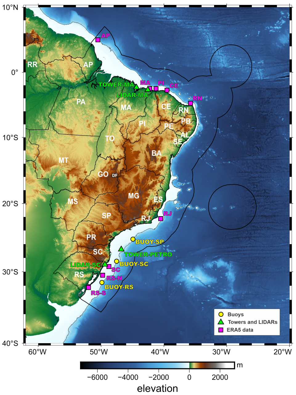
Figure 2. Study region. Magenta squares indicate the ERA5 stations (clusters) extracted for wind farm simulations. Observational points used for ERA5 validation are meteorological buoys (yellow bullets) and towers and LIDARs (green triangles). The colored bar indicates elevation in meters. The thin line represents the 500 m isobath. Coastal states with stations selected for analysis are: Amapá (AP), Maranhão (MA), Piauí (PI), Ceará (CE), Rio Grande do Norte (RN), Rio de Janeiro (RJ), Santa Catarina (SC), and Rio Grande do Sul (RS). The Exclusive Economic Zone is delimited by a thick black line. Map produced with PyGMT [52].

Figure 2. Study region. Magenta squares indicate the ERA5 stations (clusters) extracted for wind farm simulations. Observational points used for ERA5 validation are meteorological buoys (yellow bullets) and towers and LIDARs (green triangles). The colored bar indicates elevation in meters. The thin line represents the 500 m isobath. Coastal states with stations selected for analysis are: Amapá (AP), Maranhão (MA), Piauí (PI), Ceará (CE), Rio Grande do Norte (RN), Rio de Janeiro (RJ), Santa Catarina (SC), and Rio Grande do Sul (RS). The Exclusive Economic Zone is delimited by a thick black line. Map produced with PyGMT [52].

Table 1. Offshore stations selected for analysis, numbered from i = 1 to 9 (cluster). Stations’ latitudes and longitudes are indicated. A represents the amplitude, $\varphi$ the phase (rad), and M the average capacity factor, with these parameters obtained by adjusting a harmonic of 365 days period to each capacity factor time series (see Equation (2)). Capacity factors are computed from 30 years of ERA5 wind time series and application of a modern turbine power curve. All stations refer to wind farm clusters currently under environmental licensing at IBAMA, except for those indicated with a star ★ (see Figure 2).

Cluster (i)	Station *	Latitude, Longitude	A	$\mathit{\varphi }$	M
1	AP ★	5.00, −50.50	0.24	2.79	0.30
2	MA ★	−2.50, −42.25	0.29	0.32	0.47
3	PI	−2.50, −41.25	0.32	0.22	0.53
4	CE	−2.75, −39.50	0.33	−0.05	0.52
5	RN	−4.75, −35.75	0.26	−0.04	0.60
6	RJ	−22.25, −40.50	0.14	0.84	0.44
7	SC ★	−29.25, −48.75	0.10	−0.12	0.49
8	RS−N	−30.50, −49.75	0.08	0.11	0.50
9	RS−S	−32.25, −52.00	0.06	0.15	0.43

* Station locations: Amapá (AP), Maranhão (MA), Piauí (PI), Ceará (CE), Rio Grande do Norte (RN), Rio de Janeiro (RJ), Santa Catarina (SC), and Rio Grande do Sul stations north (RS-N) and south (RS-S). See Figure 2 for stations’ positions.

Table 1. Offshore stations selected for analysis, numbered from i = 1 to 9 (cluster). Stations’ latitudes and longitudes are indicated. A represents the amplitude, $\varphi$ the phase (rad), and M the average capacity factor, with these parameters obtained by adjusting a harmonic of 365 days period to each capacity factor time series (see Equation (2)). Capacity factors are computed from 30 years of ERA5 wind time series and application of a modern turbine power curve. All stations refer to wind farm clusters currently under environmental licensing at IBAMA, except for those indicated with a star ★ (see Figure 2).

Cluster (i)	Station *	Latitude, Longitude	A	$\mathit{\varphi }$	M
1	AP ★	5.00, −50.50	0.24	2.79	0.30
2	MA ★	−2.50, −42.25	0.29	0.32	0.47
3	PI	−2.50, −41.25	0.32	0.22	0.53
4	CE	−2.75, −39.50	0.33	−0.05	0.52
5	RN	−4.75, −35.75	0.26	−0.04	0.60
6	RJ	−22.25, −40.50	0.14	0.84	0.44
7	SC ★	−29.25, −48.75	0.10	−0.12	0.49
8	RS−N	−30.50, −49.75	0.08	0.11	0.50
9	RS−S	−32.25, −52.00	0.06	0.15	0.43

* Station locations: Amapá (AP), Maranhão (MA), Piauí (PI), Ceará (CE), Rio Grande do Norte (RN), Rio de Janeiro (RJ), Santa Catarina (SC), and Rio Grande do Sul stations north (RS-N) and south (RS-S). See Figure 2 for stations’ positions.

2.5. Optimization for Renewables in Power Systems

Application of optimization methods is a widespread practice in electrical power systems research, e.g., economic dispatch, coordination, reactive support allocation, Optimal Power Flow, etc. In recent years renewable sources have been the object of problem-solving through optimization with the tools available in modern systems. Rodriguez et al. (2021) used an optimization approach to wind farms combining evolutionary methods with CFD for sizing and layout of plants in a parallelogram [53]. Brennenstuhl et al. (2021) proposed a methodology for potentiating renewable sources in micro-grids with demand-side control using a GA, and applied it to a real case of a micro-grid [54]. In 2018, Neto et al. used optimization to improve the life cycle of lead–acid battery banks in micro-grids with a predominance of renewable sources [55].

Multi-objective optimization problems (Equation (3)) can be formulated as follows: find a decision variable vector $\mathbf{x}$ that satisfies a set of constraints $\mathsf{\Omega }$ and optimizes a vector function $f\left(\mathbf{x}\right)$ with components that are objective functions [56].

$$max\left[\begin{array}{c}{f}_1(x_1,x_2,x_3,x_4,...)\\ f_2(x_1,x_2,x_3,x_4,...)\\ ...\\ f_n(x_1,x_2,x_3,x_4,\dots )\end{array}\right]subjectto\mathsf{\Omega }$$

(3)

A multi-objective optimization problem can be transformed into a single-objective solution by using Pareto frontiers in the weighted-sum method, formally described by Equation (4):

$$g\left(\mathbf{x}\right)=c^{T}f\left(\mathbf{x}\right)$$

(4)

where each of the weights contained in the vector c provides importance of each objective function to the problem.

2.6. Problem Formulation

The adopted methodology aims to use a GA to reduce the power grid’s seasonal fluctuations while maintaining high energy generation levels in the long term. Specifically, the problem resides in finding the proper number of turbines ${\alpha }_i$ distributed among different wind farm clusters i subject to specific targets for a power grid $P_{grid}$. Here, the grid is simulated as expressed in Equation (5):

$$P_{grid}\left(t\right)=\sum _{i=1}^9{\alpha }_i{P}_i\left(t\right)$$

(5)

where $P_i$ represents the time series of the turbine power simulated for each cluster i listed in Table 1 based on a 30-year record (1990–2020) of wind speeds at 100 m height with an hourly time resolution. The total grid capacity in any simulation is preserved such that $\sum {\alpha }_i{P}_{max}$ = 80 GW or $\sum {\alpha }_i$ = N = 10,000 turbines (not necessarily an integer number).

For each grid simulation and ${\alpha }_i$ distribution, a least squares analysis is applied to $P_{grid}$, computed as expressed in Equation (6):

$$P_{grid}^{harm}=M_{grid}+A_{grid}cos(\omega t+{\varphi }_{grid}).$$

(6)

This provides the amplitude of the seasonal signal $A_{grid}$, the average power $M_{grid}$, and the phase ${\varphi }_{grid}$. Here, $\omega =2\pi /(365$ days). The optimization problem can then be postulated following Equation (7):

$$max\left[{\delta }_1{M}_{grid}-{\delta }_2{A}_{grid}\right]subjectto0\le \alpha \le 0.2N.$$

(7)

The goal is to maximize the average power $M_{grid}$ while reducing the seasonal amplitude $A_{grid}$. Here, ${\delta }_1$ and ${\delta }_2$ are the Pareto conditions, which weigh each of these objectives. The GA analysis returns the best (optimized) ${\alpha }_i$ combination for each ${\delta }_1$, ${\delta }_2$ prescribed pairs.

The parameters of the GA used in this paper were as follows: stopping criterion when reaching the round of 50 generations, elite population composed of 50 individuals, population composed of 1000 individuals, crossover rate of 50%, and mutation rate of 5%. Each individual represents the power distribution within the nine wind farm clusters, composed of a binary set of nine weights that can vary from 0 to 2 in steps of 2 × 10${}^{-3}$. With each weight converted into a 10-bit binary number, each individual is a 90-bit set.

The crossover criterion was made using the roulette wheel method. The operator’s result is two new individuals that randomly inherit: (i) for the first individual, a random number of bits from the first n bits of the “father” and the 90-n last bits of the “mother”, n being the random integer factor, and (ii) for the second individual, a random number of bits from the first m bits of the “mother” and the last 90-m bits of the “father”, where m is the random integer factor. The new individual is eliminated if the sum of the weights exceeds $\pm 5\%$. For the mutation operator, a random bit of the chosen individual is selected and toggled. If this bit is 0, it is converted to 1, and vice versa.

3. Results

3.1. ERA5 Validation

The observational station coordinates and wind speed statistics are listed in Table 2 along with their corresponding ERA5 neighbor point stats. The reanalysis horizontal grid resolution is near 31 km, and observation distances to ERA5 stations are less than 22 km apart. The statistics in Table 2 include the average, minimum, and maximum values, standard deviation, root mean square error, and correlation between ERA5 and observations.

The results demonstrate that ERA5 is well able to represent the wind speeds. Average winds are similar, with relative differences between 0.3 and 10%. The standard deviation, and minimum and maximum values have good agreement (Table 2).

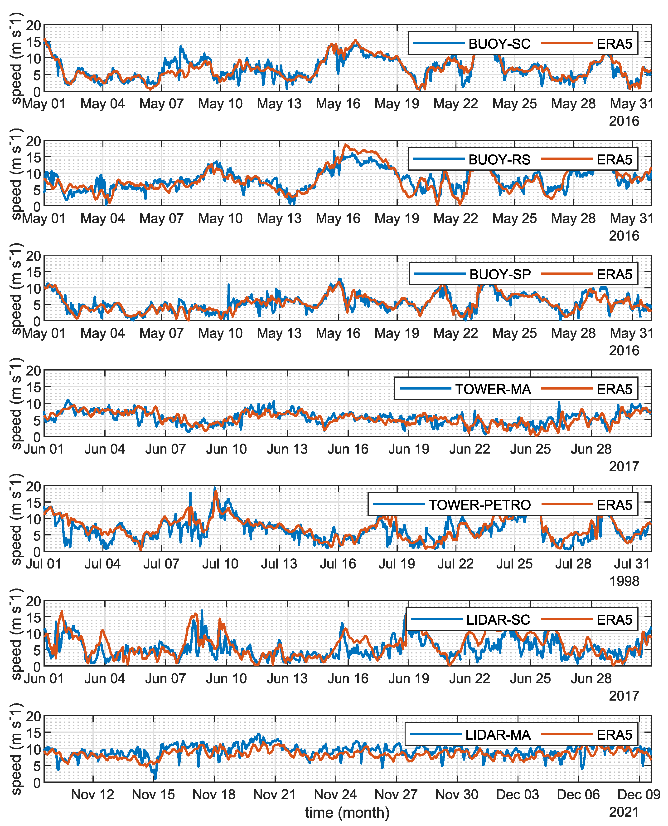
Figure 3 presents a graphic comparison of the wind speed time series with the ERA5 reanalysis. All seven stations are shown, covering 30 days. The main characteristics of the winds are well reproduced, especially in lower frequency variabilities (daily to weekly). Buoy and oceanic tower correlations vary from R = 0.70 to 0.88, while coastal station correlations vary from R = 0.57 to 0.78 (Table 2). All ERA5 stations used for comparison are situated over the ocean. However, certain observational points are located in the ocean and others (TORRE-MA, LIDAR-MA, and LIDAR-SC) in coastal areas (Table 2). These coastal points, however, present observations near hub height, which are helpful for validating ERA5.

Although winds can interact with coastal roughness elements and modify their characteristics due to heat exchange processes with the land surface, we found that in statistical terms the performance of coastal observation points was similar to ocean buoys and towers. This can probably be attributed to their proximity to the ocean, as winds at these locations continue to follow the characteristics of marine winds. TOWER-MA is nearly 300 m from the ocean, and LIDAR-MA is located 2 km from the ocean in a sandy coastal plain; both locations experience winds from the offshore quadrant and demonstrate reasonably good agreement with ERA5, with correlation (R = 0.57 to 0.78) and root mean squared errors ($RMSE$ = 1.51 to 1.80 m s⁻¹) comparable to other oceanic observational points (Table 2). LIDAR-SC is located over a fishing platform 250 m from the coast. In this region, winds tend to blow parallel to the coast [34]; nonetheless, the statistics from LIDAR-SC are encouraging, with a correlation (R = 0.72) and $RMSE$ (2.74 m s⁻¹) comparable to BUOY-RS.

Figure 3. Wind speed time series comparing observations (blue) with ERA5 reanalysis (orange). Observational data were adjusted for height. Buoy data were adjusted to 10 m and towers and LIDAR to 100 m for comparison with ERA5 data. From top to bottom, the stations are BUOY-SC, BUOY-RS, BUOY-SP, TOWER-MA, TOWER-PETRO, LIDAR-SC, and LIDAR-MA.

Figure 3. Wind speed time series comparing observations (blue) with ERA5 reanalysis (orange). Observational data were adjusted for height. Buoy data were adjusted to 10 m and towers and LIDAR to 100 m for comparison with ERA5 data. From top to bottom, the stations are BUOY-SC, BUOY-RS, BUOY-SP, TOWER-MA, TOWER-PETRO, LIDAR-SC, and LIDAR-MA.

The results in Table 2 are comparable to those of other studies. Gualtieri (2022) described median values of R = 0.86 and $RMSE$ = 2.04 m s⁻¹ for offshore stations [26]. Tavares et al. (2022) found correlations of R = 0.50 to 0.57 and $RMSE$ = 1.05 to 1.91 m s⁻¹ for buoys off Rio de Janeiro and R = 0.95 and $RMSE$ = 0.88 m s⁻¹ for a 35-m tower located on a floating oil production vessel off Brazil [28]. The close comparison of observations with ERA5 confirms the robustness of reanalysis for representing Brazilian ocean winds.

Table 2. Observational point (OBS) coordinates and statistics compared with ERA5 neighboring stations. Wind speed average, standard deviation ($std$), minimum and maximum values, root mean squared error ($RMSE$), and Pearson’s correlation coefficient (R) are listed. The column “height” lists the original data height. Whenever necessary, observations are adjusted to comparison heights of 10 m for buoys and 100 m for towers or LIDAR. The anemometer height TOWER-MA is 72 m above the ground level over a cliff that is 40 m above the sea level, making its wind measurement 112 m above the mean sea level. The distance from observational points to ERA5 grid positions is less than 22 km in all cases.

Station Name	Source	Latitude, Longitude	Average	Std	Min	Max	Height (m)	RMSE	R
BUOY−SC	ERA5	−28.5,−47.5	7.43	3.13	0.00	20.70	10.0	1.93	0.80
	OBS	−28.4897, −47.5265	7.19	2.94	0.02	20.07	3.7
BUOY−RS	ERA5	−32.5,−49.75	7.85	3.81	0.00	24.20	10.0	2.81	0.70
	OBS	−31.53933, −49.8635	7.88	3.34	0.08	24.31	3.7
BUOY−SP	ERA5	−25.25,−45	6.53	2.91	0.00	17.50	10.0	1.56	0.88
	OBS	−25.28123, −44.92697	5.82	2.59	0.03	16.61	3.7
TOWER−PETRO	ERA5	−26.75,−46.75	6.61	3.46	0.55	19.42	100.0	2.29	0.80
	OBS	−26.7667,−46.7833	7.18	3.54	0.20	18.65	78.0
TOWER−MA	ERA5	−2.25,−44.25	6.85	2.30	0.33	14.25	100.0	1.51	0.78
	OBS	−2.3189, −44.3683	6.65	2.26	0.20	13.51	72.00
LIDAR−SC	ERA5	−29,−49.25	5.98	3.60	0.67	21.13	100.0	2.74	0.72
	OBS	−28,9630, −49.38018	6.45	3.63	0.02	20.24	110.0
LIDAR−MA	ERA5	−2.50, −42.50	9.66	1.91	0.94	14.45	100.0	1.80	0.57
	OBS	−2.6941, −42.55469	8.84	1.54	2.26	13.48	100.0

Table 2. Observational point (OBS) coordinates and statistics compared with ERA5 neighboring stations. Wind speed average, standard deviation ($std$), minimum and maximum values, root mean squared error ($RMSE$), and Pearson’s correlation coefficient (R) are listed. The column “height” lists the original data height. Whenever necessary, observations are adjusted to comparison heights of 10 m for buoys and 100 m for towers or LIDAR. The anemometer height TOWER-MA is 72 m above the ground level over a cliff that is 40 m above the sea level, making its wind measurement 112 m above the mean sea level. The distance from observational points to ERA5 grid positions is less than 22 km in all cases.

Station Name	Source	Latitude, Longitude	Average	Std	Min	Max	Height (m)	RMSE	R
BUOY−SC	ERA5	−28.5,−47.5	7.43	3.13	0.00	20.70	10.0	1.93	0.80
	OBS	−28.4897, −47.5265	7.19	2.94	0.02	20.07	3.7
BUOY−RS	ERA5	−32.5,−49.75	7.85	3.81	0.00	24.20	10.0	2.81	0.70
	OBS	−31.53933, −49.8635	7.88	3.34	0.08	24.31	3.7
BUOY−SP	ERA5	−25.25,−45	6.53	2.91	0.00	17.50	10.0	1.56	0.88
	OBS	−25.28123, −44.92697	5.82	2.59	0.03	16.61	3.7
TOWER−PETRO	ERA5	−26.75,−46.75	6.61	3.46	0.55	19.42	100.0	2.29	0.80
	OBS	−26.7667,−46.7833	7.18	3.54	0.20	18.65	78.0
TOWER−MA	ERA5	−2.25,−44.25	6.85	2.30	0.33	14.25	100.0	1.51	0.78
	OBS	−2.3189, −44.3683	6.65	2.26	0.20	13.51	72.00
LIDAR−SC	ERA5	−29,−49.25	5.98	3.60	0.67	21.13	100.0	2.74	0.72
	OBS	−28,9630, −49.38018	6.45	3.63	0.02	20.24	110.0
LIDAR−MA	ERA5	−2.50, −42.50	9.66	1.91	0.94	14.45	100.0	1.80	0.57
	OBS	−2.6941, −42.55469	8.84	1.54	2.26	13.48	100.0

3.2. Seasonal Characterization

Brazil has a long continental shelf that extends for more than 7000 km from its northern limit at Amapá (4.5${}^{\circ }$ N) to the Rio Grande do Sul (33.7${}^{\circ }$ S) (Figure 2). The region is influenced by major atmospheric systems such as the Atlantic High-Pressure Center, the Intertropical Convergence Zone (ITCZ), the Trade winds, and synoptic weather systems [12,57,58,59]. Wind stations thus reflect the influence of these different atmospheric systems.

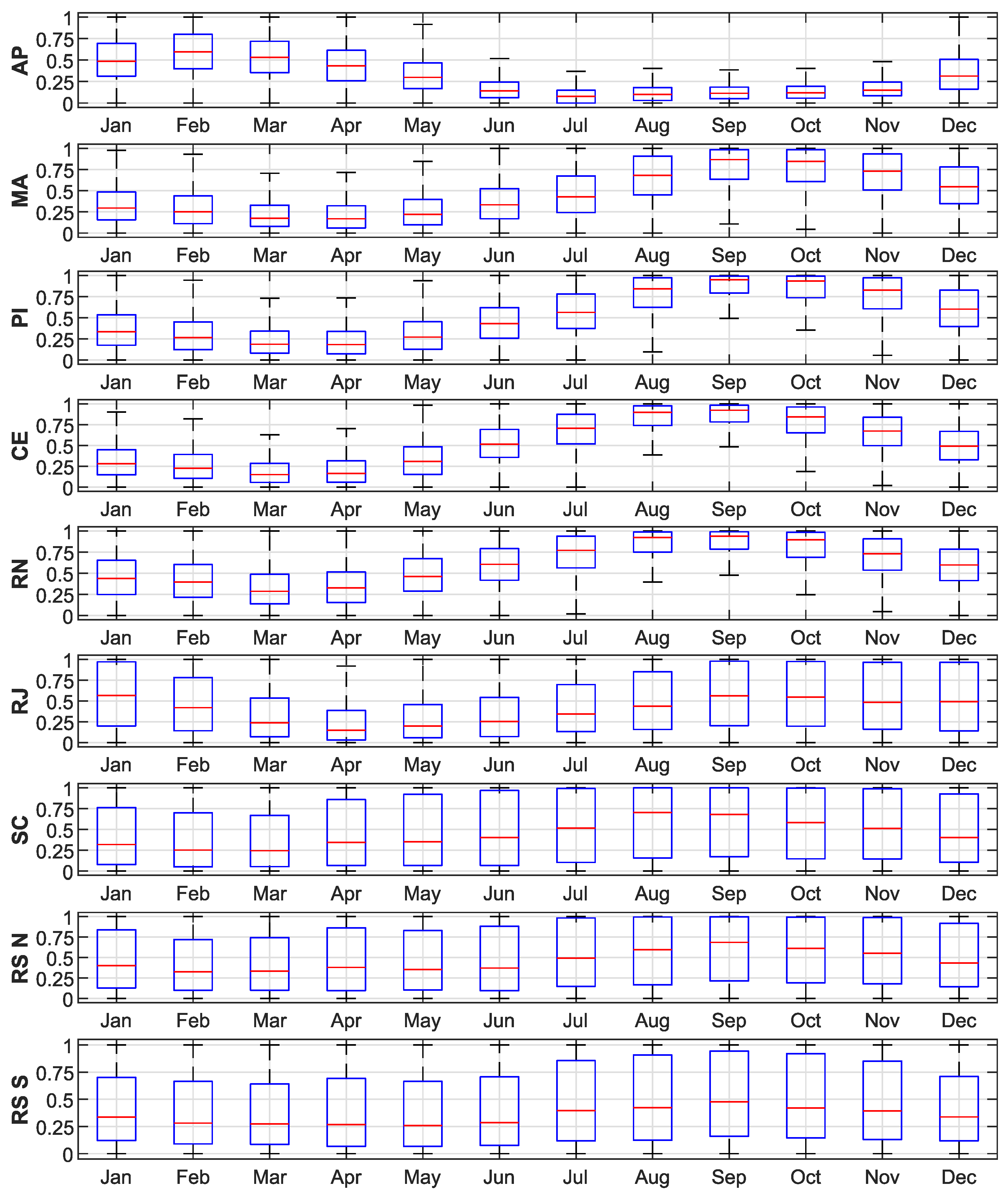
Figure 4 presents capacity factor monthly distributions for the six regions where offshore development is already planned (PI, CE, RN, RJ, RS-N, and RS-S) along with three other station sites included in this work (AP, MA, and SC). All box plots are based on 30 years of wind speed data converted to capacity factor series based on the power curve of a Vestas V164 wind turbine. The stations shown in Figure 4 are organized from AP on the top (north) to RS on the bottom (south).

The higher capacity factors occur in the northeast, including the MA, PI, CE, and RN regions. The median $CF$ peaks above 0.75 from August to November in these regions. In average, these stations have yearly capacity factors varying from 0.47 to 0.60 (Table 1).

The box plots demonstrate the presence of steadier winds in the northeast. The 25th and 75th percentiles are concentrated in a narrower range of 0.60 to 0.95. This partially explains why Brazil’s wind energy investments are focused on this region. Northeastern wind farms do not face damaging storms and present months with outstanding production and respectable yearly capacity factors.

The northeast, however, is characterized by significant seasonal amplitudes. The harmonic analysis of $CF$ results in amplitudes of A = 0.26 to 0.33 for MA, PI, CE, and RN (Table 1). With such large amplitudes, a period of weaker winds in the northeast can be reliably expected. This occurs from January to May, as shown in Figure 4, during the rainy season, when capacity factors can drop to values as low as $CF$ = 0.15.

Southern stations display less seasonal variability. The harmonic amplitude decays to A = 0.14 for RJ, and is surprisingly low, at A = 0.06, for RS-S (Table 1). The box plots, however, are usually tall. The 25th and 75th percentiles have a much wider range year-round (0.25 to 0.75). This is a result of the frequent passage of synoptic systems, such as cyclones and anticyclones [58,59]. Depending on stations’ position with respect to these atmospheric systems, they can expect alternating low or high winds in a matter of days or even hours.

Figure 4. Capacity factor monthly distributions for individual wind farm clusters at AP★, MA★, PI, CE, RN, RJ, SC★, RN-N, and RS-S. The central mark in each box is the median. Box edges are the 25th and 75th percentiles. The whiskers extend to the most extreme data points (approximately ± 2.7 $\sigma$) and 99.3 % coverage if data are normally distributed). All stations represent wind farms under environmental licensing at IBAMA except for those identified with a star (★).

Figure 4. Capacity factor monthly distributions for individual wind farm clusters at AP★, MA★, PI, CE, RN, RJ, SC★, RN-N, and RS-S. The central mark in each box is the median. Box edges are the 25th and 75th percentiles. The whiskers extend to the most extreme data points (approximately ± 2.7 $\sigma$) and 99.3 % coverage if data are normally distributed). All stations represent wind farms under environmental licensing at IBAMA except for those identified with a star (★).

Cyclones typically travel along the coast and move to the ocean, rarely migrating beyond the latitude of Rio de Janeiro. As a result, the thickness of the box plots (25th and 75th percentile differences) for the south (SC, RS-N, and RS-S) and southeast (RJ) is typically larger than for the northeast (MA, PI, CE, RN) and north (AP). Taking RS-S and PI in October as an example, in RS-S the variation is from 0.1 to 0.9, while in PI the variation is from 0.75 to 1. This is due to the strong synoptic variability present in the south of the country, whereas the Trade winds regime is active in the northeast.

In general terms, the northeastern and southern stations demonstrate lower capacity factors in the year’s first half and higher capacity factors in the second half. An outstanding exception is Amapá (AP), located in the extreme north of Brazil (Figure 1). In AP, winds present inverse behavior in terms of seasonal variability. In contrast to other stations, the first months of the year in AP have high wind intensity. Median capacity factors reach 0.5 from January to March, with thin box plot distributions, while they are less than 0.3 in MA, CE, and PI for the same months.

In the second period, however, the production starts to fall in AP, reaching shallow levels from June to November. AP has a seasonal signal of considerable amplitude, with A = 0.24, however, this is nearly 160${}^{\circ }$ out of phase with the northeastern stations (Figure A1). These contrasting patterns can be attributed to these stations’ positions relative to the Intertropical Convergence Zone (ICTZ) [12]. When the ICTZ is located to the north, near AP, the southeast trades peak in the northeast at RN, CE, PI, and MA. When the ICTZ moves southward, the northeast trades become stronger at AP, and winds at RN, CE, PI, and MA are low. This represents a synchronized phenomenon that has important implications for the grid’s seasonal stabilization.

3.3. Wind Power Correlation with Distance

An offshore grid, from the point of view of connected wind farms, can improve short-term generation fluctuations. The interconnection of distant farms can significantly reduce hourly ramps. Kempton et al. (2011) investigated wind observations off the east coast of the US, establishing a decorrelation spatial scale, where wind stations start to complement each other [15]. Martin et al. (2015) studied the geographical diversity of winds across Southeastern Australia, Canada, and the Northwestern US [60]. Solbrekke et al. (2020) investigated the mitigation of wind power intermittency in the interconnection of Norwegian offshore sites [16]. All of these studies demonstrate that short-term power fluctuations are effectively smoothed by the aggregation of wind plants across distant areas. They found that wind correlations between stations drop significantly to near zero beyond a distance of 400 to 600 km, a length that is comparable to the scale of synoptic atmospheric systems [57].

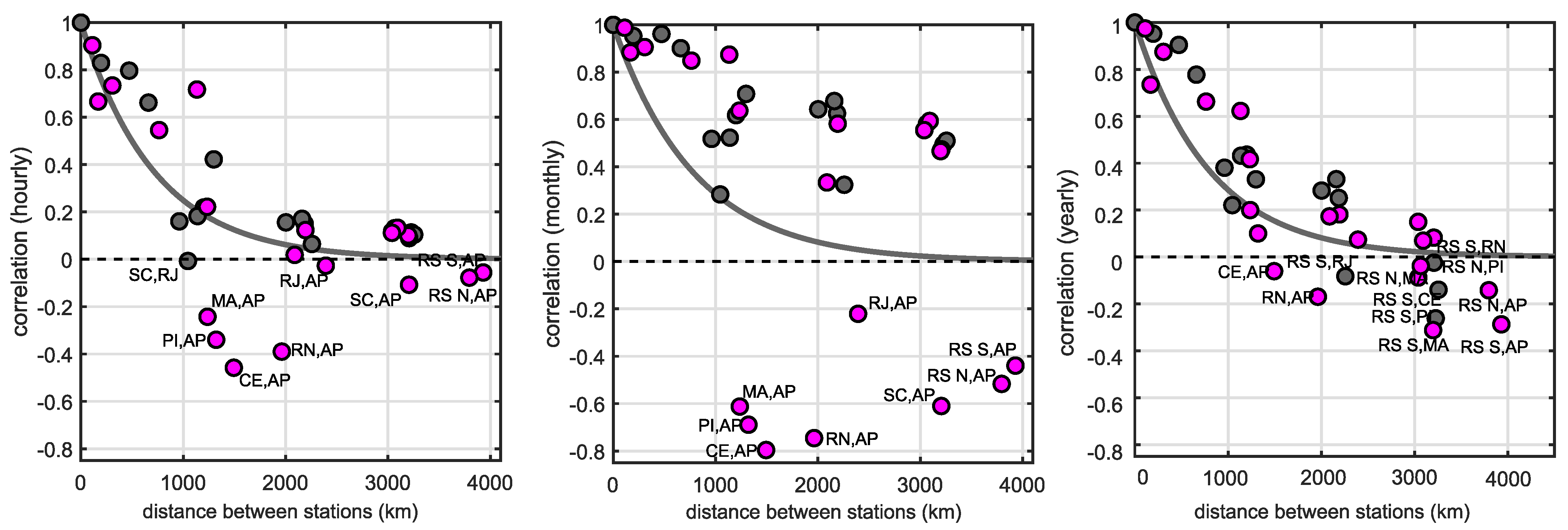
We explored the correlation between pairs of wind stations for the Brazilian offshore region using the ERA5 dataset. Correlations were calculated using the time series in terms of capacity factor. Despite this, the results of the correlations using the wind speed series are very similar. Here, all nine stations listed in Table 1 are considered for analysis (Figure 5). The gray points identify correlations within the six clusters of wind farms already under environmental analysis by IBAMA. The magenta points involve pairings with one of the stations suggested in this work (AP, MA, or SC). The three different panels in Figure 5 illustrate the scatter distributions of the correlations computed from hourly, monthly, and yearly time series.

Analysis of the gray points computed from hourly time series illustrate the expectation based on previous works [15,16,60] (Figure 5, left panel). The bullets at 0 distance and 1 correlation represent all nine stations, each correlated with itself. The correlation drops relatively fast as wind stations are compared to neighboring locations. A gray line illustrates the exponential fit of the function $R=exp(-d/D)$, where D represents an e-folding decaying spatial scale. As the curve demonstrates, correlations drop near zero for distances beyond 2000 km. This suggests that aggregating distant wind turbines can smooth hourly ramps, significantly improving grid generation.

The magenta points in Figure 5 illustrate correlations with the AP station. They stand out due to their negative correlations −0.5 < R < −0.2 at distances between 1000 < d < 2000 km. This behavior corresponds to the seasonal complementarity of AP and MA, PI, CE, and RN stations described in the previous section. Slightly negative correlations occur for the RJ, SC, and RS pairings with AP as well.

Surprisingly, when exploring the correlations employing monthly or yearly time series, negative correlations hold for the AP pairings. As a matter of fact, the correlations with AP reach $R=-0.8$ for CE, $R<-0.6$ for MA, PI, and RN, and $R<-0.4$ for SC and RS at the monthly time scale (Figure 5, center panel). Yearly time series hold negative correlations, suggesting that AP might be complementary to the northeastern and southern stations on an interannual basis.

These scatter distributions present relevant information for decision-making, leading to the concept of Reserve Wind Power plants. The role of reserve plants is normally attributed to dispatchable power sources such as thermal plants. In this case, we show that by arranging a significant amount of RWP turbines in AP, the problem of seasonal fluctuations in the grid can be alleviated.

Figure 5. Correlation R between pairs of stations as a function of geographical distance d. The panels illustrate correlation distributions for hourly, monthly, and yearly time series averages (1990–2020). The gray points identify correlations between the clusters of wind farms already under environmental licensing at IBAMA, while the magenta points identify correlations with the stations (AP, MA or SC) suggested in this work. A gray curve represents these points’ exponential fit, R = exp(−d/D). The decorrelation spatial scale D is 719.75 km for hourly, 800 km for monthly, and 800 km for yearly time series.

Figure 5. Correlation R between pairs of stations as a function of geographical distance d. The panels illustrate correlation distributions for hourly, monthly, and yearly time series averages (1990–2020). The gray points identify correlations between the clusters of wind farms already under environmental licensing at IBAMA, while the magenta points identify correlations with the stations (AP, MA or SC) suggested in this work. A gray curve represents these points’ exponential fit, R = exp(−d/D). The decorrelation spatial scale D is 719.75 km for hourly, 800 km for monthly, and 800 km for yearly time series.

3.4. Offshore Grid Simulation

For the simulation of the offshore grid, we initially focused on the performance of the offshore farms currently under analysis at IBAMA. These are the PI, CE, RN, RJ, RS-N, and RS-S wind clusters listed in Table 1 and Figure 2. The Vestas V164 power curve was selected as a reference for power calculation, even though other models are considered in the original wind farm projects [50]. Here, the turbine distribution is calculated based on the summed capacity of each wind farm cluster.

Each cluster capacity distribution is listed in Table 3, here identified as the “baseline” simulation. This represents 2.38 GW of wind turbines on the PI coast, 16.82 GW in CE, 12.78 GW in RN, 24.53 GW in RJ, 13.06 GW in RS-N, and 10.4 GW in RS-S, for a total of 80 GW. The AP, MA, and SC wind farms are assigned 0 GW in this initial simulation, as none of these locations are considered in the projects under environmental licensing at IBAMA (as presented in January 2022).

The turbine power $P_i\left(t\right)$ is evaluated for each cluster from ERA5 data. The number of turbines ${\alpha }_i$ can be computed by dividing the local installed capacity by 8 MW, the nameplate capacity of the Vestas V164 (Table 3). Calculation of $P_{grid}$ then follows Equation (5).

The panels in Figure 6a illustrate the $P_{grid}$ time series (left panel) and histogram distribution (right panel). A thin orange line presents the daily averages of the grid (computed from hourly data), and a darker brown line presents the monthly means. Daily to seasonal ramps can be identified. Peak production is above 70 GW, while the lowest production is sometimes below 10 GW. The grid, however, never reaches 0 GW. A strong seasonal signal is identified in this grid simulation, as large wind clusters are considered for the northeast and RJ.

Table 3 summarizes the performance of this baseline simulation. The grid’s overall capacity factor is $CF$ = 0.48, with average power of $M_{grid}$ = 39.1 GW. The total energy over the simulated 30 year period is 9588 TWh. The amplitude of the seasonal fluctuation is $A_{grid}$ = 13.7 GW, which represents 35% of the grid’s average power (Table 3).

These results demonstrate an improvement compared to the performance of isolated wind parks. By aggregating distant (uncorrelated) wind farms, periods of no generation become absent and periods below 10%$CF$ (8 GW) occur 1.12% of the time. The histogram distribution demonstrates that this hypothetical grid operates between 10 and 70 GW on most days, with modal distribution around 40 GW (Figure 6a, right panel). This type of analysis is highly simplified, as it does not include wind turbine distributions around the clusters, wake losses, failures, maintenance periods, or transmission losses.

3.5. Offshore Grid Optimization

The performance of the “baseline” grid explored in the previous section leads to the problem of optimization. Key questions to be answered here are: (i) the most significant energy production that can be achieved; (ii) the minimum seasonal variability that can be reproduced; and (iii) whether there is an optimal distribution of the maximum energy generation and minimum seasonal power amplitude.

The problem formulated in Section 2.6 allows for the investigation of these questions based on the choice of ${\delta }_1$, ${\delta }_2$ parameters and the history of $P_i$ at these locations. All wind farm clusters listed in Table 1 are considered for this analysis, including AP, MA, and SC. These three suggested stations were included in the grid optimization based on the seasonal and spatial correlation analysis performed on Section 3.2 and Section 3.3, respectively.

Table 3 describes the results for six rounds of simulation after GA optimization, varying the Pareto value from ${\delta }_1$ = 1, ${\delta }_2$ = 0 to ${\delta }_1$ = 0, ${\delta }_2$ = 1 in 0.2 increments. For each simulation, the sum of Pareto is always unity. Equation (7) establishes the ${\delta }_1$ weights for total energy generation (average power), while ${\delta }_2$ minimizes the seasonal amplitude of $P_{grid}$.

Table 3. Results for offshore grid simulation and optimization. Baseline refers to the distribution of wind farms currently under environmental licensing at IBAMA. The other cases refer to the results of grid optimization. Here, ${\delta }_1$ weights are used for total power generation, while ${\delta }_2$ minimizes the seasonal amplitude of $P_{grid}$. For each Pareto pair, the GA finds the optimized ${\alpha }_i$ distribution of wind turbines for each farm cluster. $A_{grid}$ is the seasonal amplitude, $M_{grid}$ is the average production of the power grid ($P_{grid}$) in GW units, $CF$ refers to the mean capacity factor of the grid, and $E30$ refers to the generated energy in TWh integrated from $P_{grid}$ for a 30-year simulation period. The installed capacity of each cluster ($AP$ to $RS$-S) is presented in GW units.

Simulation	${\mathit{A}}_{\mathit{grid}}$	${\mathit{M}}_{\mathit{grid}}$	$\mathit{CF}$	$\mathit{E}30$	$\mathit{AP}$	$\mathit{MA}$	$\mathit{PI}$	$\mathit{CE}$	$\mathit{RN}$	$\mathit{RJ}$	$\mathit{SC}$	$\mathit{RS}$-N	$\mathit{RS}$-S
baseline	13.75	39.08	0.48	9588	0.0	0.0	2.38	16.82	12.78	24.53	0.0	13.06	10.4
${\delta }_1$ = 1.0, ${\delta }_2$ = 0.0	15.92	40.32	0.50	9891	0.75	12.51	10.35	7.91	12.57	10.97	12.40	12.02	0.52
${\delta }_1$ = 0.8, ${\delta }_2$ = 0.2	8.19	37.73	0.47	9256	13.44	0.82	5.32	6.35	14.36	4.48	10.91	12.37	11.95
${\delta }_1$ = 0.6, ${\delta }_2$ = 0.4	5.43	36.09	0.45	8854	14.67	0.21	3.08	2.76	6.44	10.79	14.38	14.49	13.18
${\delta }_1$ = 0.4, ${\delta }_2$ = 0.6	5.57	35.29	0.44	8659	16.13	6.18	4.02	2.05	1.72	8.06	13.47	14.59	13.78
${\delta }_1$ = 0.2, ${\delta }_2$ = 0.8	5.22	35.79	0.45	8780	17.13	1.74	1.29	3.68	5.91	14.13	17.48	13.61	5.04
${\delta }_1$ = 0.0, ${\delta }_2$ = 1.0	5.09	35.34	0.44	8670	15.68	0.89	5.91	0.87	2.49	11.37	17.07	10.91	14.83

Station locations: Amapá (AP), Maranhão (MA), Piauí (PI), Ceará (CE), Rio Grande do Norte (RN), Rio de Janeiro (RJ), Santa Catarina (SC), and Rio Grande do Sul stations north (RS-N) and south (RS-S). See Figure 2 for positions.

Table 3. Results for offshore grid simulation and optimization. Baseline refers to the distribution of wind farms currently under environmental licensing at IBAMA. The other cases refer to the results of grid optimization. Here, ${\delta }_1$ weights are used for total power generation, while ${\delta }_2$ minimizes the seasonal amplitude of $P_{grid}$. For each Pareto pair, the GA finds the optimized ${\alpha }_i$ distribution of wind turbines for each farm cluster. $A_{grid}$ is the seasonal amplitude, $M_{grid}$ is the average production of the power grid ($P_{grid}$) in GW units, $CF$ refers to the mean capacity factor of the grid, and $E30$ refers to the generated energy in TWh integrated from $P_{grid}$ for a 30-year simulation period. The installed capacity of each cluster ($AP$ to $RS$-S) is presented in GW units.

Simulation	${\mathit{A}}_{\mathit{grid}}$	${\mathit{M}}_{\mathit{grid}}$	$\mathit{CF}$	$\mathit{E}30$	$\mathit{AP}$	$\mathit{MA}$	$\mathit{PI}$	$\mathit{CE}$	$\mathit{RN}$	$\mathit{RJ}$	$\mathit{SC}$	$\mathit{RS}$-N	$\mathit{RS}$-S
baseline	13.75	39.08	0.48	9588	0.0	0.0	2.38	16.82	12.78	24.53	0.0	13.06	10.4
${\delta }_1$ = 1.0, ${\delta }_2$ = 0.0	15.92	40.32	0.50	9891	0.75	12.51	10.35	7.91	12.57	10.97	12.40	12.02	0.52
${\delta }_1$ = 0.8, ${\delta }_2$ = 0.2	8.19	37.73	0.47	9256	13.44	0.82	5.32	6.35	14.36	4.48	10.91	12.37	11.95
${\delta }_1$ = 0.6, ${\delta }_2$ = 0.4	5.43	36.09	0.45	8854	14.67	0.21	3.08	2.76	6.44	10.79	14.38	14.49	13.18
${\delta }_1$ = 0.4, ${\delta }_2$ = 0.6	5.57	35.29	0.44	8659	16.13	6.18	4.02	2.05	1.72	8.06	13.47	14.59	13.78
${\delta }_1$ = 0.2, ${\delta }_2$ = 0.8	5.22	35.79	0.45	8780	17.13	1.74	1.29	3.68	5.91	14.13	17.48	13.61	5.04
${\delta }_1$ = 0.0, ${\delta }_2$ = 1.0	5.09	35.34	0.44	8670	15.68	0.89	5.91	0.87	2.49	11.37	17.07	10.91	14.83

Station locations: Amapá (AP), Maranhão (MA), Piauí (PI), Ceará (CE), Rio Grande do Norte (RN), Rio de Janeiro (RJ), Santa Catarina (SC), and Rio Grande do Sul stations north (RS-N) and south (RS-S). See Figure 2 for positions.

The results for the first optimization simulation, with ${\delta }_1$ = 1, ${\delta }_2$ = 0, are illustrated in Figure 6b. Again, the orange line represents $P_{grid}$ daily power variability (averaged from hourly data) and the brown line represents the monthly averages. Comparing this case with the “baseline”, these simulations are quite similar.

For optimization, the average power is $M_{grid}$ = 40.32 GW, compared to $M_{grid}$ = 39.08 GW in the baseline simulation. In terms of energy generated over the 30 years, the figures are $E30$ = 9891 TWh and 9588 TWh, respectively. The capacity factors are $CF$ = 0.50 and 0.48, respectively, for the two cases (Table 3). This suggests that the GA slightly improves the energy generation performance (4 %), indicating that the present offshore wind farms proposed at IBAMA are nearly optimized for maximum power generation with little room for improvement. This can be interpreted as a result of investment in sites with large yearly $CF$, which guarantees the most substantial energy yield. Both grids, however, suffer from large seasonal amplitudes: $A_{grid}$ = $13.75$ GW for the baseline against $A_{grid}$ = 15.92 for the ${\delta }_1$ = 1, ${\delta }_2$ = 0 simulation. The GA results for this Pareto frontier enjoy the advantage of more distributed farms along the coast. In the baseline case, the installed capacity in the RJ cluster alone is 24.53 GW.

Figure 6. Results of the offshore grid simulations. The left-hand panels represent the time series of $P_{grid}$ for 30 years (GW units). The thin orange line represents daily averages computed from hourly data and the thicker brown line represents monthly averages. The right-hand panels indicate the correspondent histogram (PDF, blue bars) and cumulative distributions (1-CDF, orange line) of $P_{grid}$. The rows indicate (a) the baseline simulation including all offshore wind parks currently proposed at IBAMA, (b) GA optimization for maximum power generation, and (c) GA optimization for the minimum seasonal amplitude of $P_{grid}$.

Figure 6. Results of the offshore grid simulations. The left-hand panels represent the time series of $P_{grid}$ for 30 years (GW units). The thin orange line represents daily averages computed from hourly data and the thicker brown line represents monthly averages. The right-hand panels indicate the correspondent histogram (PDF, blue bars) and cumulative distributions (1-CDF, orange line) of $P_{grid}$. The rows indicate (a) the baseline simulation including all offshore wind parks currently proposed at IBAMA, (b) GA optimization for maximum power generation, and (c) GA optimization for the minimum seasonal amplitude of $P_{grid}$.

The pursuit of minimal seasonal fluctuation can be explored by setting ${\delta }_1$ = 0 and ${\delta }_2$ = 1 (Table 3). The GA optimization results are illustrated in Figure 6c for this Pareto pair. Comparing this case with the maximum generation simulation, it is clear that $P_{grid}$ seasonal amplitudes are significantly reduced. The seasonal amplitude of the grid falls from $A_{grid}$ = 15.92 GW to $A_{grid}$ = 5.09 GW, barely one third of the previous Pareto simulation (Table 3). The average power of the grid $M_{grid}$ is 35.34 GW and the $CF$ is 0.44, representing a 9% reduction in terms of energy compared to a 68% beneficial reduction in terms of the seasonal power amplitude of the grid.

An important distinction is the larger daily variability observable in Figure 6c compared to Figure 6a,b. This results from the larger allocation of turbines in the southern regions, where there is substantial synoptic activity. An incremental distribution of these wind farms around their clusters along the RS and SC coasts should reduce hourly to daily power ramps, as suggested by previous works [15,16,60]. This problem, however, was not pursued further in this work.

The question remains, however, whether better intermediary situations might arise from the choice of Pareto ${\delta }_1$ and ${\delta }_2$. These results are summarized on Table 3. When the focus is maximum energy generation (${\delta }_1$ = 1 and ${\delta }_2$ = 0), optimization reserves less than 1 GW for AP, although it distributes wind turbines more fairly among MA, PI, and SC. AP is not an appropriate place to compete with wind farms with high yearly capacity factors, as its yearly capacity factor is $CF$ = 0.3.

On the other hand, as the Pareto ${\delta }_2$ grows, a significant reduction in the seasonal amplitude $A_{grid}$ follows, with an acceptable penalty for energy. As example, for the Pareto condition ${\delta }_1=0.6$ and ${\delta }_2=0.4$, the seasonal amplitude is minimized by 66% compared to Pareto ${\delta }_1$ = 1, with a penalty of only 10% to the mean power. For this condition, the power allocated to the AP is substantial (14.7 GW).

For a 30-year wind series, the current proposition (baseline) would mean power below 10% of installed capacity (8 GW) 3% of the time, while with maximum energy optimization this percentage is 2% and for the above Pareto value (${\delta }_1=0.6$ and ${\delta }_2=0.4$) it is less than 1%.

The PDF power distributions demonstrate that the first two solutions extend up to the minimum and maximum values of the power grid. On the other hand, a more centralized distribution with fewer low power and high power periods results in ${\delta }_2$ gaining importance (Figure 6c, right panel). As the seasonal amplitude of the time series decays, the histograms reveal that power variability occurs within a much narrower envelope (20 to 60 GW) compared to the baseline simulation.

It is worth mentioning that the objective function of the optimization problem is a nonlinear multivariable problem, meaning that the final results may be local optimal solutions which depend on the starting conditions of the iterative method.

3.6. Reserve Wind Power Plants

The power balance is one of the most basic principles that guarantee the system’s safety. All power systems are susceptible to events that risk the balance between load and generation [61]. Although certain systems allow load shedding at particular times or even incorporate it into energy contracts with foreseen remuneration, a smarter alternative is to use reserve sources. These sources increase system reliability and guarantee its safety, as the system operator can activate it in cases where there is any disturbance in the system. However, as power systems have been modernized alternatives such as static storage systems and green hydrogen are increasingly being studied.

For the time being, thermoelectric power plants are the basis of reserve energy contracts. They can be dispatched anytime to compensate for disturbances caused in the grid by load increases or generation variability. On the other hand, there is an urgent need to reduce the use of these sources, as they are large GHG emitters and low emission options are currently unfeasible from an economic point of view. Based on these facts and the results presented in the previous sections, the concept of RWP plants can be introduced.

RWP plants are analogous to the use of thermal power plants. Under this concept, offshore wind sites would be evaluated not only through their yearly capacity factor and power amplitudes, but also based on the possibility of delivering power during critical months when other wind farms experience low wind regimes. This can be accomplished by installing wind turbines in strategic areas characterized by negative correlations. Figure 4 clearly illustrates the concept of a possible RWP in the AP region; while in the first four months of the year the $CF$ is substantially reduced at other sites in Brazil, in AP it presents much better performance.

It is helpful to quantify the feasibility of RWP using present energy market values. The levelized cost of energy (LCOE) for a gas peaker (usually used as a reserve power supplier) in Brazil ranges between 208 and 246 USD/MWh [62]. Prices for onshore wind power plants vary from 30 to 49 USD/MWh. As mentioned before, the offshore wind energy market is in an early stage in Brazil, meaning that prices for these sources are unknown. However, worldwide values are 66 to 100 USD/MWh, with average values around 83 USD/MWh [62].

Among all sites concerned here, AP is the worst in terms of yearly capacity factor ($CF$ = 0.30), which makes it unattractive for investors from the point of view of yearly revenue. However, when considering the RWP concept, AP has half of the RN capacity factor simulated for 30 years (see Table 1). Considering similar costs over a lifetime, AP would provide half of the expected yearly generation of RN, implying an LCOE of 166 USD/MWh. This would make AP approximately 20 to 32% cheaper than thermal reserve plants, with the additional advantage of being a source that contributes to decarbonization goals.

From this point of view, it is evident that yearly $CF$ is not the only parameter that should be considered when assessing offshore wind power investment; comparison to thermal sources makes such plants much more interesting from a development perspective. In terms of cost, Wiser et al. [63] anticipate that offshore costs should decline by 17–35% in 2035 and 37–49% in 2050. Median LCOE values of 60 USD/MWh are expected for 2025 and 50 USD/MWh for 2030 (see Figure 4 in Wiser et al., 2021 [63]). Within these optimistic scenarios, RWPs makes even more sense from an economic and environmental perspective.

4. Summary and Conclusions

In this study, we investigated the performance of hypothetical offshore wind farms based on 30 years of wind speeds derived from ERA5 reanalysis. Winds were used to compute the aggregate generation of turbines anticipated for projects under environmental licensing in Brazil. A total of nine stations, from Amapá (AP) state in the north to the Rio Grande do Sul state (RS) in the south, were selected for analysis, including areas not yet considered for offshore development.

The stations presented substantial meteorological diversity. The northern and northeastern stations are under the influence of the Intertropical Convergence Zone (ITCZ) and the Trade winds regime; they display large seasonal amplitudes, with peak windy seasons centered on Jan-Feb-Mar in the north and Aug-Sep-Oct in the northeast. The southeastern and southern stations are dominated by the Atlantic High-Pressure Center, with the frequent passage of synoptic weather systems. As a result, they experience milder seasonal variability and significant daily to weekly variability.

The regional complementarity of different wind regimes was explored by computing the correlation of neighboring and remote wind stations. A striking result was the strong negative correlations (R = −0.8) encountered between the northern station in Amapá (AP) and the stations in Rio Grande do Norte (RN). This outcome is due to Trade wind variability and ITCZ migration [11,12]. Negative correlations also hold for the northern (AP) and the southeastern and southern stations.

Simulation of an offshore grid was performed for a baseline scenario (based on current proposals), maximum generation and for seasonal optimization of the system. The results demonstrate that the relocation of wind turbines can reduce the seasonal amplitude by 68% while incurring a penalty of only 9% to average power generation. This is accomplished by the inclusion of the northern region and redistribution of wind farms based on a genetic algorithm.

Other studies have addressed the importance of large-scale deployment for improved generation. Kempton et al. (2011) demonstrated that interconnection of wind farms on the U.S. east coast should reduce the variance and rate of change of power while eliminating hours of null production [15]. Grams et al. (2017) demonstrated how the exploration of peripheral regions of Europe in northern Scandinavia, Iberia, and the Balkans has high potential for electricity generation during severe lulls in the North Sea [64]. Both studies, however, were focused on mid-latitude weather-regimes and employed strategies to balance the hourly to multi-daily variability of winds.

The results presented here demonstrate that the exploration of wind resources along Brazil’s tropical and subtropical regions can help to stabilize wind generation on a seasonal scale. A simple method based on paired correlations helped to identify strongly complementary regimes.

These findings are significant, as there is time to establish policies encouraging offshore investment and diversification. The high complementarity of the north station with other regions lead us to the concept of Reserve Wind Power (RWP) plants. These farms can be viewed as “reserve sources” for energy security, and can replace contracts with thermal reserve plants, with concurrent economic and environmental advantages. Our analysis suggests that RWP plants can be 20 to 32% cheaper than thermal reserves using current market values.

Although the seasonal stabilization of the grid was a clear outcome of our analysis, the results of our simulations should be used with caution. The spatial distribution of wind turbines around the selected stations (clusters) was not considered, meaning that the simulated hourly to daily variability is probably overestimated. Parametrization of turbine wakes and consideration of other economic aspects such as foundation and transmission line costs would further improve this work. This represents a preliminary large-scale simulation of wind farms based on reanalysis data, and the fine details of wind fields near the coast were not considered. The numerical downscaling of ERA5 with weather prediction models could provide a better description of winds, resolve orographic effects, and permit the study of wakes from individual wind turbines or entire wind parks. Validation of regional models depends on wind observations at the height of the turbines, which at present are scarce for the region studied here. Related studies would benefit from more extensive field programs for measuring wind profiles in coastal and oceanic areas of Brazil.

References

- Lu, X.; McElroy, M.B.; Kiviluoma, J. Global potential for wind-generated electricity. Proc. Natl. Acad. Sci. USA 2009, 106, 10933–10938. [Google Scholar] [CrossRef] [PubMed]
- Marvel, K.; Kravitz, B.; Caldeira, K. Geophysical limits to global wind power. Nat. Clim. Chang. 2013, 3, 118–121. [Google Scholar] [CrossRef]
- GWEC. Global Wind Report | Gwec; Technical Report; GWEC: Brussels, Belgium, 2021. [Google Scholar]
- Wiser, R.; Jenni, K.; Seel, J.; Baker, E.; Hand, M.; Lantz, E.; Smith, A. Expert elicitation survey on future wind energy costs. Nat. Energy 2016, 1, 1–8. [Google Scholar] [CrossRef]
- Beiter, P.; Rand, J.T.; Seel, J.; Lantz, E.; Gilman, P.; Wiser, R. Expert perspectives on the wind plant of the future. Wind Energy 2022, 25. [Google Scholar] [CrossRef]
- Islam, S. Challenges and opportunities in grid connected commercial scale PV and wind farms. In Proceedings of the 9th International Conference on Electrical and Computer Engineering, ICECE 2016, Dhaka, Bangladesh, 20–22 December 2016; pp. 1–7. [Google Scholar] [CrossRef]
- Gross, R.; Green, T.; Leach, M.; Skea, J.; Heptonstall, P.; Anderson, D. The Costs and Impacts of Intermittency: An Assessment of the Evidence on the Costs and Impacts of Intermittent Generation on the British Electricity Network; UK Energy Research Centre: London, UK, 2006; p. 112. [Google Scholar]
- Rahimi, E.; Rabiee, A.; Aghaei, J.; Muttaqi, K.M.; Esmaeel Nezhad, A. On the management of wind power intermittency. Renew. Sustain. Energy Rev. 2013, 28, 643–653. [Google Scholar] [CrossRef]
- Pfenninger, S.; Hawkes, A.; Keirstead, J. Energy systems modeling for twenty-first century energy challenges. Renew. Sustain. Energy Rev. 2014, 33, 74–86. [Google Scholar] [CrossRef]
- Pimenta, F.M.; Assireu, A.T. Simulating reservoir storage for a wind-hydro hydrid system. Renew. Energy 2015, 76, 757–767. [Google Scholar] [CrossRef]
- Silva, A.R.; Pimenta, F.M.; Assireu, A.T.; Spyrides, M.H.C. Complementarity of Brazil’s hydro and offshore wind power. Renew. Sustain. Energy Rev. 2016, 56, 413–427. [Google Scholar] [CrossRef]
- Pimenta, F.M.; Silva, A.R.; Assireu, A.T.; Almeida, V.d.S.e.; Saavedra, O.R. Brazil Offshore Wind Resources and Atmospheric Surface Layer Stability. Energies 2019, 12, 4195. [Google Scholar] [CrossRef] [Green Version]
- Cazzaro, D.; Trivella, A.; Corman, F.; Pisinger, D. Multi-scale optimization of the design of offshore wind farms. Appl. Energy 2022, 314, 118830. [Google Scholar] [CrossRef]
- Sinden, G. Characteristics of the UK wind resource: Long-term patterns and relationship to electricity demand. Energy Policy 2007, 35, 112–127. [Google Scholar] [CrossRef]
- Kempton, W.; Pimenta, F.M.; Veron, D.E.; Colle, B.A. Electric power from offshore wind via synoptic-scale interconnection. Proc. Natl. Acad. Sci. USA 2010, 107, 7240–7245. [Google Scholar] [CrossRef] [PubMed]
- Solbrekke, I.M.; Kvamstø, N.G.; Sorteberg, A. Mitigation of offshore wind power intermittency by interconnection of production sites. Wind Energy Sci. 2020, 5, 1663–1678. [Google Scholar] [CrossRef]
- Olauson, J. ERA5: The new champion of wind power modelling? Renew. Energy 2018, 126, 322–331. [Google Scholar] [CrossRef]
- Berger, M.; Radu, D.; Dubois, A.; Pandžić, H.; Dvorkin, Y.; Louveaux, Q.; Ernst, D. Siting renewable power generation assets with combinatorial optimisation. Optim. Lett. 2022, 16, 877–907. [Google Scholar] [CrossRef]
- Radu, D.; Berger, M.; Dubois, A.; Fonteneau, R.; Pandžić, H.; Dvorkin, Y.; Louveaux, Q.; Ernst, D. Assessing the impact of offshore wind siting strategies on the design of the European power system. Appl. Energy 2022, 305, 117700. [Google Scholar] [CrossRef]
- Pryor, S.; Barthelmie, R.; Shepherd, T.; Hahmann, A.; Garcia Santiago, O. Wakes in and between very large offshore arrays. J. Phys. Conf. Ser. 2022, 2265, 022037. [Google Scholar] [CrossRef]
- Shakoor, R.; Hassan, M.Y.; Raheem, A.; Rasheed, N. Wind farm layout optimization using area dimensions and definite point selection techniques. Renew. Energy 2016, 88, 154–163. [Google Scholar] [CrossRef]
- Barthelmie, R.J.; Hansen, K.; Frandsen, S.T.; Rathmann, O.; Schepers, J.G.; Schlez, W.; Phillips, J.; Rados, K.; Zervos, A.; Politis, E.S.; et al. Modelling and measuring flow and wind turbine wakes in large wind farms offshore. Wind Energy 2009, 12, 431–444. [Google Scholar] [CrossRef]
- Draxl, C.; Clifton, A.; Hodge, B.M.; McCaa, J. The wind integration national dataset (wind) toolkit. Appl. Energy 2015, 151, 355–366. [Google Scholar] [CrossRef]
- Hahmann, A.N.; S = ıle, T.; Witha, B.; Davis, N.N.; Dörenkämper, M.; Ezber, Y.; García-Bustamante, E.; González-Rouco, J.F.; Navarro, J.; Olsen, B.T.; et al. The making of the New European Wind Atlas–part 1: Model sensitivity. Geosci. Model Dev. 2020, 13, 5053–5078. [Google Scholar] [CrossRef]
- Sheridan, L.M.; Krishnamurthy, R.; Gorton, A.M.; Shaw, W.J.; Newsom, R.K. Validation of reanalysis-based offshore wind resource characterization using lidar buoy observations. Mar. Technol. Soc. J. 2020, 54, 44–61. [Google Scholar] [CrossRef]
- Gualtieri, G. Analysing the uncertainties of reanalysis data used for wind resource assessment: A critical review. Renew. Sustain. Energy Rev. 2022, 167, 112741. [Google Scholar] [CrossRef]
- Pronk, V.; Bodini, N.; Optis, M.; Lundquist, J.K.; Moriarty, P.; Draxl, C.; Purkayastha, A.; Young, E. Can reanalysis products outperform mesoscale numerical weather prediction models in modeling the wind resource in simple terrain? Wind Energy Sci. 2022, 7, 487–504. [Google Scholar] [CrossRef]
- de Assis Tavares, L.F.; Shadman, M.; de Freitas Assad, L.P.; Estefen, S.F. Influence of the WRF model and atmospheric reanalysis on the offshore wind resource potential and cost estimation: A case study for Rio de Janeiro State. Energy 2022, 240, 122767. [Google Scholar] [CrossRef]
- Hersbach, H.; Bell, B.; Berrisford, P.; Horányi, A.; Sabater, J.M.; Nicolas, J.; Radu, R.; Schepers, D.; Simmons, A.; Soci, C.; et al. Global reanalysis: Goodbye ERA-Interim, hello ERA5. ECMWF Newsl. 2019, 159, 17–24. [Google Scholar]
- Hersbach, H.; Bell, B.; Berrisford, P.; Hirahara, S.; Horányi, A.; Muñoz-Sabater, J.; Nicolas, J.; Peubey, C.; Radu, R.; Schepers, D.; et al. The ERA5 global reanalysis. Q. J. R. Meteorol. Soc. 2020, 146, 1999–2049. [Google Scholar] [CrossRef]
- Ramon, J.; Lledó, L.; Torralba, V.; Soret, A.; Doblas-Reyes, F.J. What global reanalysis best represents near-surface winds? Q. J. R. Meteorol. Soc. 2019, 145, 3236–3251. [Google Scholar] [CrossRef]
- Pimenta, F.M.; Kempton, W.; Garvine, R. Combining meteorological stations and satellite data to evaluate the offshore wind power resource of Southeastern Brazil. Renew. Energy 2008, 33, 2375–2387. [Google Scholar] [CrossRef]
- Nassif, F.B.; Pimenta, F.M.; D’aquino, C.d.A.; Assireu, A.T.; Garbossa, L.H.P.; Passos, J.C. Coastal wind measurements and power assessment using a lidar on a pier. Rev. Bras. De Meteorol. 2020, 35, 255–268. [Google Scholar] [CrossRef]
- Pires, C.H.M.; Pimenta, F.M.; D’Aquino, C.A.; Saavedra, O.R.; Mao, X.; Assireu, A.T. Coastal wind power in southern santa catarina, Brazil. Energies 2020, 13, 5197. [Google Scholar] [CrossRef]
- Gisler, C.A.F.; Fisch, G.; Correa, C.d.S. Análise estatística do perfil de vento na camada limite superficial no Centro de Lançamento de Alcântara. J. Aerosp. Technol. Manag. 2011, 3, 193–201. [Google Scholar] [CrossRef]
- Marciotto, E.R.; Fisch, G.; Medeiros, L.E. Characterization of surface level wind in the Centro de Lançamento de Alcântara for use in rocket structure loading and dispersion studies. J. Aerosp. Technol. Manag. 2012, 4, 69–80. [Google Scholar] [CrossRef]
- Marciotto, E.; Fisch, G. Investigation of Approaching Ocean Flow and its Interaction with Land Internal Boundary Layer. Am. J. Environ. Eng. 2013, 3, 18–23. [Google Scholar] [CrossRef]
- Medeiros, L.E.; Magnago, R.d.O.; Fisch, G.; Marciotto, E.R. Observational study of the surface layer at an ocean-land transition region. J. Aerosp. Technol. Manag. 2013, 5, 449–458. [Google Scholar] [CrossRef]
- Bonavita, M.; Hólm, E.; Isaksen, L.; Fisher, M. The evolution of the ECMWF hybrid data assimilation system. Q. J. R. Meteorol. Soc. 2016, 142, 287–303. [Google Scholar] [CrossRef]
- Dee, D.P.; Uppala, S.M.; Simmons, A.J.; Berrisford, P.; Poli, P.; Kobayashi, S.; Andrae, U.; Balmaseda, M.A.; Balsamo, G.; Bauer, P.; et al. The ERA-Interim reanalysis: Configuration and performance of the data assimilation system. Q. J. R. Meteorol. Soc. 2011, 137, 553–597. [Google Scholar] [CrossRef]
- Gelaro, R.; McCarty, W.; Suárez, M.J.; Todling, R.; Molod, A.; Takacs, L.; Randles, C.A.; Darmenov, A.; Bosilovich, M.G.; Reichle, R.; et al. The modern-era retrospective analysis for research and applications, version 2 (MERRA-2). J. Clim. 2017, 30, 5419–5454. [Google Scholar] [CrossRef]
- Kobayashi, S.; Ota, Y.; Harada, Y.; Ebita, A.; Moriya, M.; Onoda, H.; Onogi, K.; Kamahori, H.; Kobayashi, C.; Endo, H.; et al. The JRA-55 reanalysis: General specifications and basic characteristics. J. Meteorol. Soc. Jpn. Ser. II 2015, 93, 5–48. [Google Scholar] [CrossRef]
- Kalnay, E.; Kanamitsu, M.; Kistler, R.; Collins, W.; Deaven, D.; Gandin, L.; Iredell, M.; Saha, S.; White, G.; Woollen, J.; et al. The NCEP/NCAR 40-year reanalysis project. Bull. Am. Meteorol. Soc. 1996, 77, 437–472. [Google Scholar] [CrossRef]
- Ramon, J.; Lledó, L.; Pérez-Zanón, N.; Soret, A.; Doblas-Reyes, F.J. The Tall Tower Dataset: A unique initiative to boost wind energy research. Earth Syst. Sci. Data 2020, 12, 429–439. [Google Scholar] [CrossRef]
- de Assis Tavares, L.F.; Shadman, M.; de Freitas Assad, L.P.; Silva, C.; Landau, L.; Estefen, S.F. Assessment of the offshore wind technical potential for the Brazilian Southeast and South regions. Energy 2020, 196, 117097. [Google Scholar] [CrossRef]
- Saha, S.; Moorthi, S.; Wu, X.; Wang, J.; Nadiga, S.; Tripp, P.; Behringer, D.; Hou, Y.T.; Chuang, H.y.; Iredell, M.; et al. The NCEP climate forecast system version 2. J. Clim. 2014, 27, 2185–2208. [Google Scholar] [CrossRef]
- Hayes, L.; Stocks, M.; Blakers, A. Accurate long-term power generation model for offshore wind farms in Europe using ERA5 reanalysis. Energy 2021, 229, 120603. [Google Scholar] [CrossRef]
- Patel, R.P.; Nagababu, G.; Kachhwaha, S.S.; Surisetty, V.V.K. A revised offshore wind resource assessment and site selection along the Indian coast using ERA5 near-hub-height wind products. Ocean Eng. 2022, 254, 111341. [Google Scholar] [CrossRef]
- Lange, B.; Larsen, S.; Højstrup, J.; Barthelmie, R. Importance of thermal effects and sea surface roughness for offshore wind resource assessment. J. Wind Eng. Ind. Aerodyn. 2004, 92, 959–988. [Google Scholar] [CrossRef]
- IBAMA. Offshore Wind Complexes. Projects with Open Environmental Licensing Processes at IBAMA; Technical Report; Brazilian Institute of Environment and Renewable Natural Resources: Brasília, Brazil, 2022. Available online: http://www.ibama.gov.br/laf/consultas/mapas-de-projetos-em-licenciamento-complexos-eolicos-offshore (accessed on 22 February 2022).
- Thomson, R.E.; Emery, W.J. Data Analysis in Physical Oceanography, 3rd ed.; Wiley Series in Discrete Mathematics and Optimization; Wiley: Amsterdam, The Netherlands, 2014. [Google Scholar]
- Uieda, L.; Tian, D.; Leong, W.J.; Jones, M.; Schlitzer, W.; Grund, M.; Toney, L.; Yao, J.; Magen, Y.; Materna, K.; et al. PyGMT: A Python interface for the Generic Mapping Tools. 2022. Available online: https://www.pygmt.org/latest/ (accessed on 10 September 2022). [CrossRef]
- Gonzalez-Rodriguez, A.G.; Serrano-González, J.; Burgos-Payán, M.; Riquelme-Santos, J.M. Realistic Optimization of Parallelogram-Shaped Offshore Wind Farms Considering Continuously Distributed Wind Resources. Energies 2021, 14, 2895. [Google Scholar] [CrossRef]
- Brennenstuhl, M.; Lust, D.; Pietruschka, D.; Schneider, D. Demand Side Management Based Power-to-Heat and Power-to-Gas Optimization Strategies for PV and Wind Self-Consumption in a Residential Building Cluster. Energies 2021, 14, 6712. [Google Scholar] [CrossRef]
- Neto, P.B.L.; Saavedra, O.R.; de Souza Ribeiro, L.A. A dual-battery storage bank configuration for isolated microgrids based on renewable sources. IEEE Trans. Sustain. Energy 2018, 9, 1618–1626. [Google Scholar] [CrossRef]
- Chong, E.; Zak, S. An Introduction to Optimization; Wiley Series in Discrete Mathematics and Optimization; Wiley: Hoboken, NJ, USA, 2013. [Google Scholar]
- Wallace, J.M.; Hobbs, P.V. Atmospheric science: An Introductory Survey; Elsevier: Amsterdam, The Netherlands, 2006; Volume 92. [Google Scholar]
- de Jesus, E.M.; da Rocha, R.P.; Crespo, N.M.; Reboita, M.S.; Gozzo, L.F. Multi-model climate projections of the main cyclogenesis hot-spots and associated winds over the eastern coast of South America. Clim. Dyn. 2021, 56, 537–557. [Google Scholar] [CrossRef]
- Crespo, N.M.; da Rocha, R.P.; Sprenger, M.; Wernli, H. A potential vorticity perspective on cyclogenesis over centre-eastern South America. Int. J. Climatol. 2021, 41, 663–678. [Google Scholar] [CrossRef]
- Clara, M.S.; Martin, J.K.L.; Handschy, M.A. Variability of interconnected wind plants: Correlation length and its dependence on variability time scale. Environ. Res. Lett. 2015, 10, 044004. [Google Scholar] [CrossRef]
- Wood, A.J.; Wollenberg, B.F.; Sheblé, G.B. Power Generation, Operation, and Control; John Wiley & Sons: Hoboken, NJ, USA, 2013. [Google Scholar]
- Lazard’s Levelized Cost of Energy Analysis-Version 15.0. Technical Report. 2021. Available online: https://www.lazard.com/media/451086/lazards-levelized-cost-of-energy-version-130-vf.pdf (accessed on 1 September 2022).
- Wiser, R.; Rand, J.; Seel, J.; Beiter, P.; Baker, E.; Lantz, E.; Gilman, P. Expert elicitation survey predicts 37% to 49% declines in wind energy costs by 2050. Nat. Energy 2021, 6, 555–565. [Google Scholar] [CrossRef]
- Grams, C.M.; Beerli, R.; Pfenninger, S.; Staffell, I.; Wernli, H. Balancing Europe’s wind-power output through spatial deployment informed by weather regimes. Nat. Clim. Chang. 2017, 7, 557–562. [Google Scholar] [CrossRef] [Green Version]
Figure 1.
Flowchart of analysis, including data sources, validation, methods of analysis, power grid simulation, and optimization.
Publisher’s Note: MDPI stays neutral with regard to jurisdictional claims in published maps and institutional affiliations. |
© 2022 by the authors. Licensee MDPI, Basel, Switzerland. This article is an open access article distributed under the terms and conditions of the Creative Commons Attribution (CC BY) license (https://creativecommons.org/licenses/by/4.0/).
Share and Cite
MDPI and ACS Style
Fernandes, I.; Pimenta, F.M.; Saavedra, O.R.; Assireu, A.T. Exploring the Complementarity of Offshore Wind Sites to Reduce the Seasonal Variability of Generation. Energies 2022, 15, 7182. https://doi.org/10.3390/en15197182
AMA Style
Fernandes I, Pimenta FM, Saavedra OR, Assireu AT. Exploring the Complementarity of Offshore Wind Sites to Reduce the Seasonal Variability of Generation. Energies. 2022; 15(19):7182. https://doi.org/10.3390/en15197182
Chicago/Turabian StyleFernandes, Italo, Felipe M. Pimenta, Osvaldo R. Saavedra, and Arcilan T. Assireu. 2022. "Exploring the Complementarity of Offshore Wind Sites to Reduce the Seasonal Variability of Generation" Energies 15, no. 19: 7182. https://doi.org/10.3390/en15197182
Note that from the first issue of 2016, this journal uses article numbers instead of page numbers. See further details here.