


Hybrid MLI Topology Using Open-End Windings for Active Power Filter Applications

Faculty of Engineering, Electrical Engineering Department, King Saud University, Riyadh 12372, Saudi Arabia
*
Author to whom correspondence should be addressed.
Energies 2022, 15(17), 6434; https://doi.org/10.3390/en15176434
Submission received: 21 May 2022
/
Revised: 14 July 2022
/
Accepted: 29 July 2022
/
Published: 2 September 2022
(This article belongs to the Special Issue Electrical Power Engineering and Renewable Energy Technologies)
Abstract
:Different multilevel converter topologies have been presented for achieving more output voltage steps, hence improving system performance and lowering costs. In this paper, a hybrid multilevel inverter (MLI) topology is proposed for active-power-filter applications. The proposed MLI is a combination of two standard topologies: the cascaded H-bridge and the three-phase cascaded voltage source inverter. This configuration enhances the voltage levels of the proposed MLI while using fewer switches than typical MLI topologies. The proposed MLI was developed in the MATLAB/Simulink environment, and a closed-loop control technique was used to achieve a unity power factor connection of the PV modules to the grid, as well as to compensate for harmonics caused by nonlinear loads. To demonstrate that the configuration was working correctly and that the control was precise, the proposed MLI was constructed in a laboratory. A MicroLabBox real-time controller handled data acquisition and switch gating. The proposed topology was experimentally connected to the grid and the MLI was experimentally used as an active power filter to compensate for the harmonics generated due to nonlinear loads. This control technique was able to generating a sinusoidal grid current that was in phase with the grid voltage, and the grid current’s total harmonic distortion was within acceptable limits. To validate the practicability of the proposed MLI, both simulation and experimental results are presented.
1. Introduction
Multilevel inverter (MLI) topologies have attracted interest in a variety of applications, including grid-connected PV applications, static VAR compensators, and active-power-filter (APF) applications. MLIs have many advantages over conventional inverters, such as reducing the total harmonic distortion (THD) of the produced voltage and current, reducing the size of filters, reducing the switching frequency, and improving the inverter efficiency [1]. Many cascaded inverter topologies have been proposed in the literature [2]. Of these, cascaded H-bridge (CHB) topologies have advantages over other MLI topologies (e.g., layout simplicity, extreme modularity, and construction and control simplicity) because they are free of voltage-balance issues. Moreover, compared to other MLI topologies, CHB topologies use the fewest components at the same voltage levels [3,4]. Asymmetrical CHB topologies have been proposed in which the DC voltages are not symmetrical. The combination of these asymmetrical DC voltages results in the generation of increased voltage levels [5,6]. On the other hand, hybrid MLI topologies presented in the literature have been based on a three-phase voltage source inverter (VSI) unit with a CHB. In these topologies, H-bridge units are coupled to floating capacitors whose voltages must be carefully regulated. This complicates the control algorithm [7,8].
Recently, research into the development of APF applications has increased [9,10]. APFs are electronic devices that can be accurately used to eliminate the harmonic contents in a current. The harmonics in power systems can be created by nonlinear loads connected to the public grid. Some of these loads are computers with a switched-mode power supply, motor drives, and electronic light ballasts (fax machines, medical equipment, etc.). These harmonics may cause unwanted effects, such as heating of sensitive electrical equipment or of the generators and transformers, which leads to increased core loss and may cause transformer and equipment failure, random circuit breaker tripping, flickering lights, high neutral currents due to zero sequence harmonics, and conductor losses [11]. As a result, these harmonics must be eliminated. There are three different types of harmonic filters: passive, active, and hybrid. The advantages of APFs over passive filters are numerous. They can, for example, suppress supply-current harmonics as well as reactive currents. On the other hand, certain harmonics will involve their own passive filter, hence there will be more passive filters needed if there are more harmonics to remove. Because only large harmonics with lower frequencies are usually removed, the filters will be bulky due to the geometric size of the inductor [12]. In contrast to passive power filters, APFs can eliminate any harmonics by using a suitable control and the performance of APFs is unaffected by the characteristics of the power distribution system [9,11,13,14].
Several APF topologies using the conventional three-phase VSI have been proposed [15,16,17]. In addition, some of the proposed APFs were based on the classical three-level H-bridge inverter [18]. Recently, the use of MLI topologies in APF applications has become a hot topic [19,20]. An APF based on a seven-level neutral-point clamped (NPC) MLI was proposed in [21]. The authors used LS–PWM and fuzzy control approaches to eliminate current harmonics generated by nonlinear loads. Others [19] used a three-level NPC for active-power-filter applications. The authors used a fuzzy-logic controller and a fractional-order proportional-integral (PI) controller to control the proposed system. From another point of view, an APF based on a three level NPC-T type was proposed in [20,22]. The authors in [23] proposed a five-level HB-NPC MLI for APF applications with an experimental validation. Other authors used a CHB for APF applications due it the advantages of the CHB such as simplicity and possession of a high modularity [24,25]. Both CHN topologies were proposed for APFs either by directly connecting the H-bridges in series or by cascading the H-bridges using transformers [26,27,28]. Moreover, cascaded MLI topologies are used for APF applications [29,30]. The authors in [30] proposed a shunt APF based on cascaded MLI topology using a single power source with three-phase transformers. The proposed scheme could adjust for polluted loads with high harmonics and a poor power factor. To compute compensating currents, the dq theory was applied. A prototype was built to validate the simulation results by the experimental results.
In this paper, a hybrid MLI topology is proposed for APF applications. The proposed MLI topology conjoins the cascaded H-bridge MLI and the cascaded three-phase VSI topology using open-end windings and was first proposed and tested under different load parameters, as presented in [31]. In addition, this new topology has been patented, as seen in [32]. However, the previous paper focused only on the topology itself. The topology was not used in any applications. This paper is the first to detail the utilization of the new topology for the active power filter and for grid-connected PVs. The proposed MLI is used to compensate the harmonic currents of the nonlinear load, while the grid supplies the fundamental positive-sequence currents of the load. A closed-loop control is proposed for both applications—the APF and the PV–grid connection. Finally, the proposed MLI was experimentally implemented in the lab, and it was tested for the two applications.
2. The Proposed Hybrid Active-Power-Filter Topology
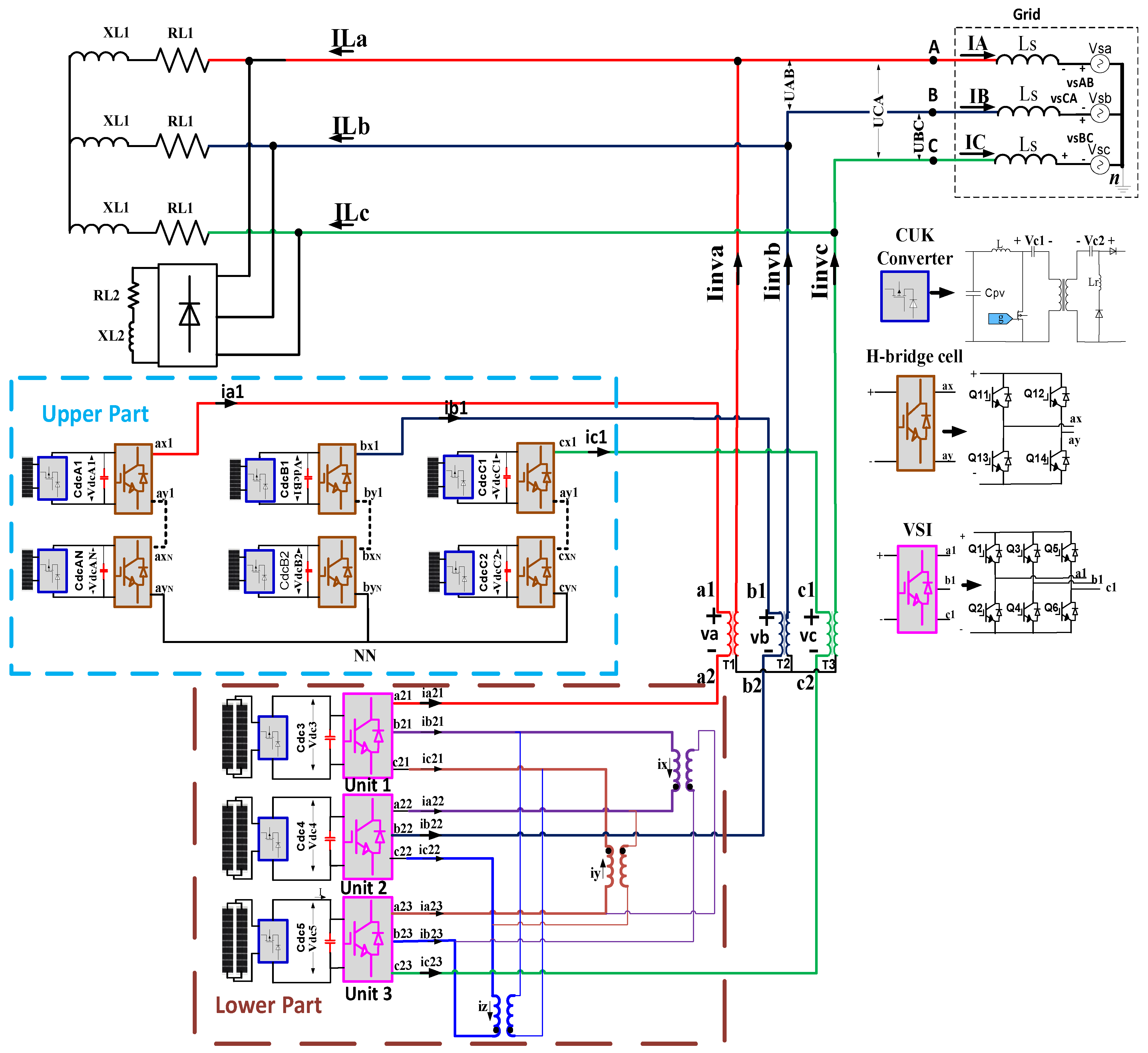
A three-phase multilevel high-voltage/high-power converter is used in this topology. It is a hybrid arrangement that combines two common multilevel configurations: a cascaded H-bridge MLI and a three-phase cascaded VSI. These two configurations are joined together to create the hybrid configuration. Figure 1 depicts the suggested cascaded MLI architecture. This novel topology has been given a patent with the number US 10, 141, 865 B1. It is suitable for a wide variety of grid-connected applications, including power-factor correction, static-VAR compensation, and grid-connected photovoltaic (PV) systems. The proposed architecture is made up of two components linked by an open-end windings transformer.
As shown in this figure, the proposed MLI is capable of supplying the extracted PV power to the nonlinear loads and of injecting power into the grid. The idea is to compensate the harmonics generated by the nonlinear loads while supplying balanced three-phase currents to the grid. The control scheme proposed in [33] has been extended to be used for the proposed APF in this paper. The proposed control scheme is used to inject balanced three-phase low harmonic currents into the grid. If the three-phase loads are nonlinear, then the load currents will contain harmonics, which may reduce the current quality of the grid. Therefore, the harmonic contents of the load currents must be extracted to be compensated by the MLI. Consequently, the grid current will be balanced and contain low harmonic contents. The current of the nonlinear loads may contain positive-, negative-, or zero-sequence harmonics.
Therefore, the following steps are considered:
- Extract the fundamental positive-sequence component of the load current using the following equation:
- 2.
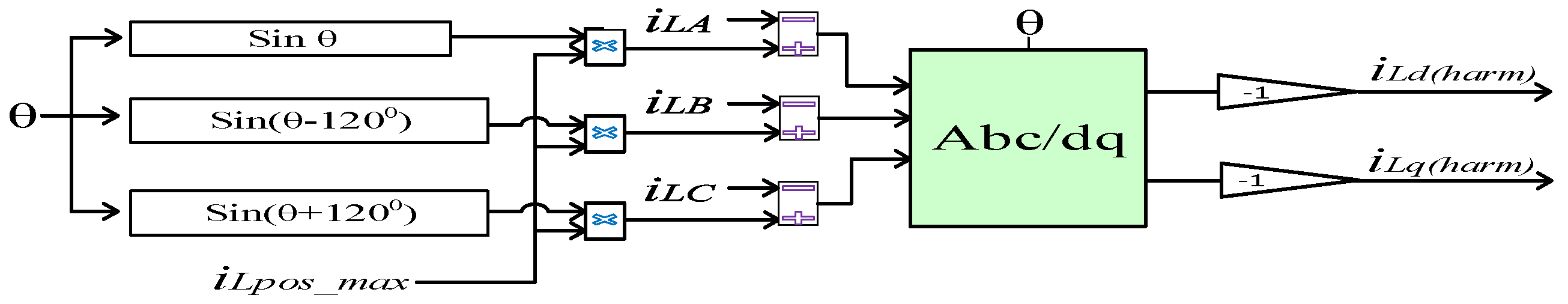
- The maximum value of the fundamental component of the load current is extracted, and the harmonic contents of the load currents can be extracted by the following equation:
- 3.
- The extracted harmonic components of the load currents are then converted into a dq frame as shown in Figure 2.
From another perspective, the main goal of the control scheme is to produce reference currents that deliver only available active power to the grid while maintaining unity power factor. The DC links share the same active phase grid currents. These DC-link voltages are compared to their respective reference voltages.
If the DC-link voltages are accurately regulated by the control system, then:
where are the corresponding DC-link voltages of the phases a, b, and c, respectively.
The d-q components of the terminal voltages of the proposed MLI are given by:
The sequential function is given by:
The DC link current is defined as follows:
Analyzing nonlinearity problems requires presention of a new model. These inputs could be written as:
To ensure the unity power factor, the reactive current in Equation (6) should be set to zero. Therefore,
In normal operation the following properties apply:
where is the maximum grid voltage. Substituting Equation (8) in (9) yields:
The active current,, is used to regulate the DC-link capacitors. As shown in Equation (10), the active reference current can be given as:
The reference active current of the grid is the sum of the three active currents:
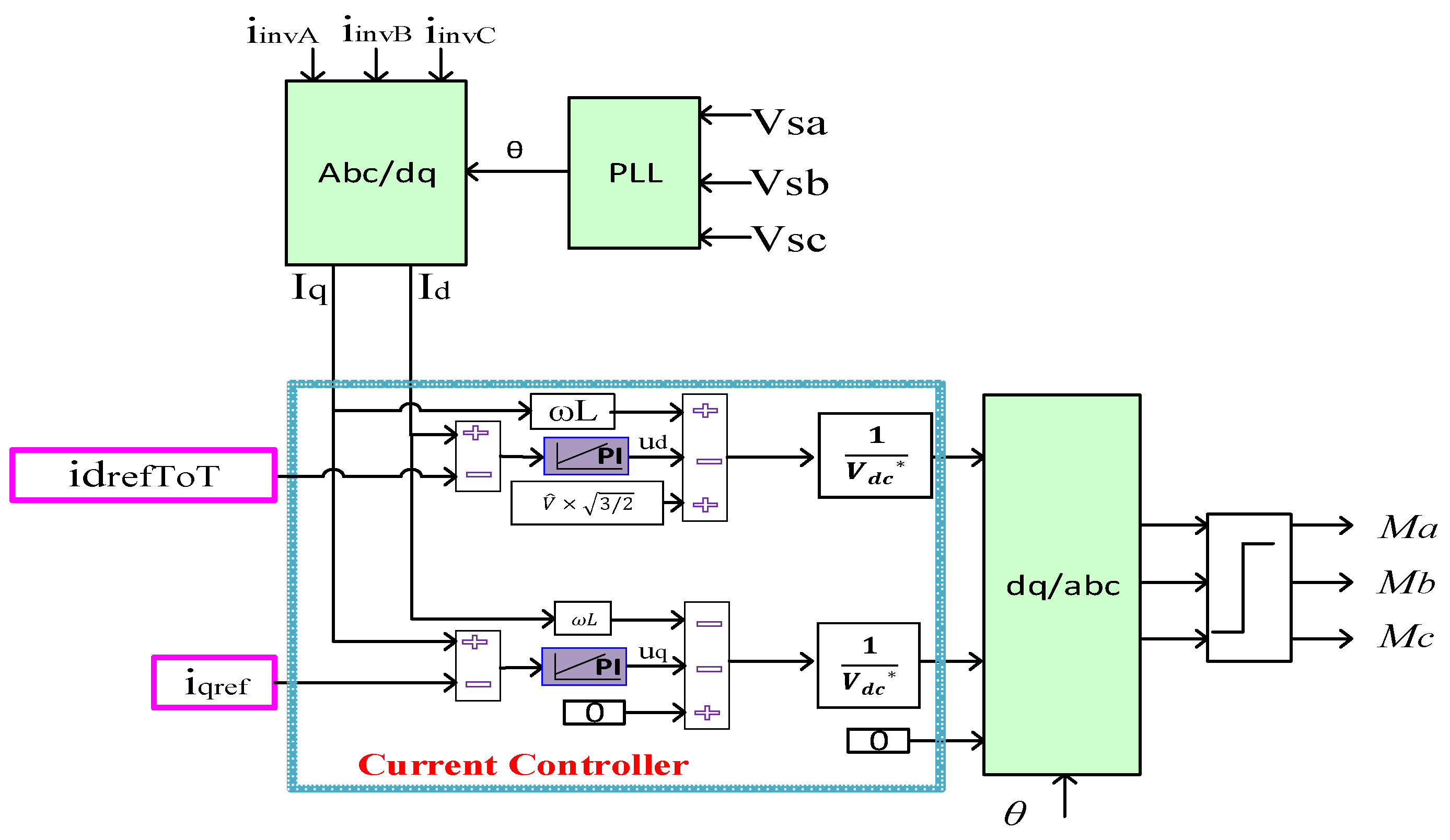
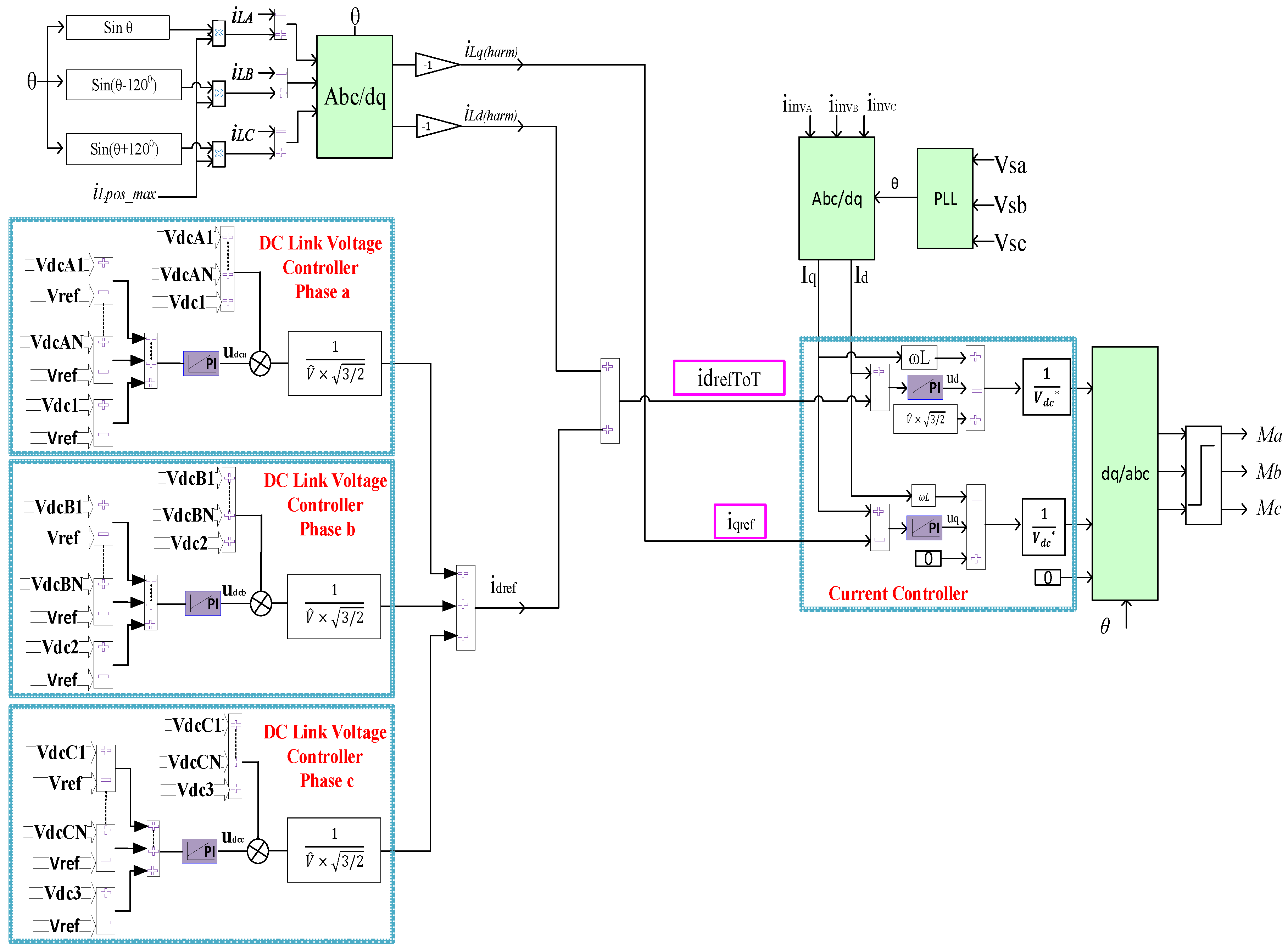
The DC-link voltage controllers of the proposed topology based on the analysis above can be seen in Figure 3. As seen in the analysis, the resulting signal from the DC-link controllers is the reference active current of the inverter,. The inner current controller can be seen in Figure 4.
Where the proposed MLI is used in a PV application, the reference active grid current is compared with the actual grid current, and the reference grid reactive current is compared with the actual reactive grid current to ensure unity power factor. However, where the proposed MLI is used in an APF application, the harmonic load current in the d axes given from Figure 2 is then added to the reference current in the d axes generated form the DC-link controllers. The total reference inverter currents are given as:
Equation (13) states that the reference active current of the inverter equals the active current produced by the DC-links and the active harmonic load current. The complete proposed control scheme for APF application can be seen in Figure 5.
According to the proposed control scheme, two cases can be applied:
- 1.
- The proposed inverter acts as an active filter only.
The reference currents of the inverter are the harmonic load currents. The inverter is responsible for compensating the harmonic load currents while the grid supplies the fundamental positive-sequence currents of the load.
- 2.
- The proposed inverter is responsible for delivering the PV power to the grid and the load.
If there is enough power at the DC side, e.g., from the PV modules, the control system drives the inverter to supply the balanced positive-sequence current to the grid, as well as supplies the active load current and compensates harmonic load currents.
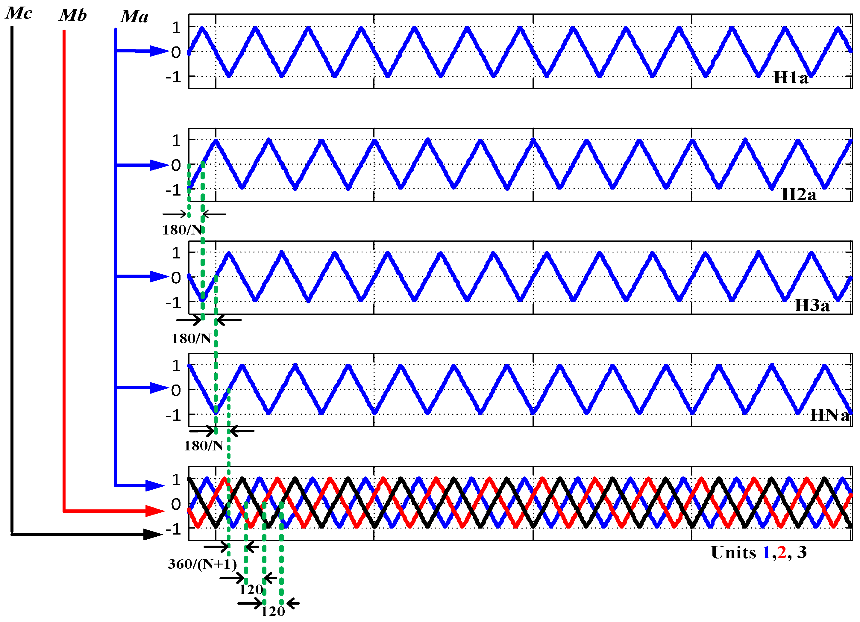
In both cases, Equation (13) is applied to perform the current control stage. The load current harmonics are then transferred into the dq frame (Figure 2). These currents are then used as reference MLI currents, which are then used in Equation (13). The resulting signals from Figure 4, and , obtained from Equation (7), are then transformed into abc reference frame (. These values are then compared to the triangle carrier waveforms in Figure 6 to create switching pulses to operate the IGBTs of the proposed hybrid MLI. To produce the required pulses for the IGBTs of the upper part of the proposed MLI, the carrier waveform of the is shifted from the by 180°/N. Only the carrier waveforms of phase a in the upper part are displayed in Figure 5. Moreover, the modulation waveforms are also used to fire the IGBTs of the lower part in the proposed configuration by comparing them with the phase-shifted carrier signals, as seen in Figure 6. The carrier signal, which is used to generate the pulses of unit 2, is shifted by (T/3) from that of unit 1, and the carrier signal of unit 3 is shifted by (T/3) from that of unit 2.
3. Simulation Results
The proposed topology was built in the SIMULINK environment. For simplicity, two H-bridge units were used per phase in the proposed topology. The system consisted of 12 HIT-N220A01 PV modules; six of them were connected to upper part of the proposed topology such that one PV module was linked to each H-bridge unit. The other six PV modules were connected to the lower part of the proposed MLI such that two parallel PV modules were linked to each VSI unit. Two cases were used in the simulation:
- A.
- Grid-Connected PV Application Case
The system parameters used for simulation are shown in Table 1, while Table 2 shows the PV module parameters. The nonlinear load is disconnected from Figure 1. Therefore, no harmonic current term is applied in Equation (2). The reference reactive current of the inverter was set to zero to guarantee unity power factor. The proposed topology was used only to connect the PV modules to the grid. The perturb and observe (P & O) algorithm was used to extract the maximum power from the PV modules. The closed-loop control scheme shown in Figure 3 and Figure 4 was used for grid-connection purposes.
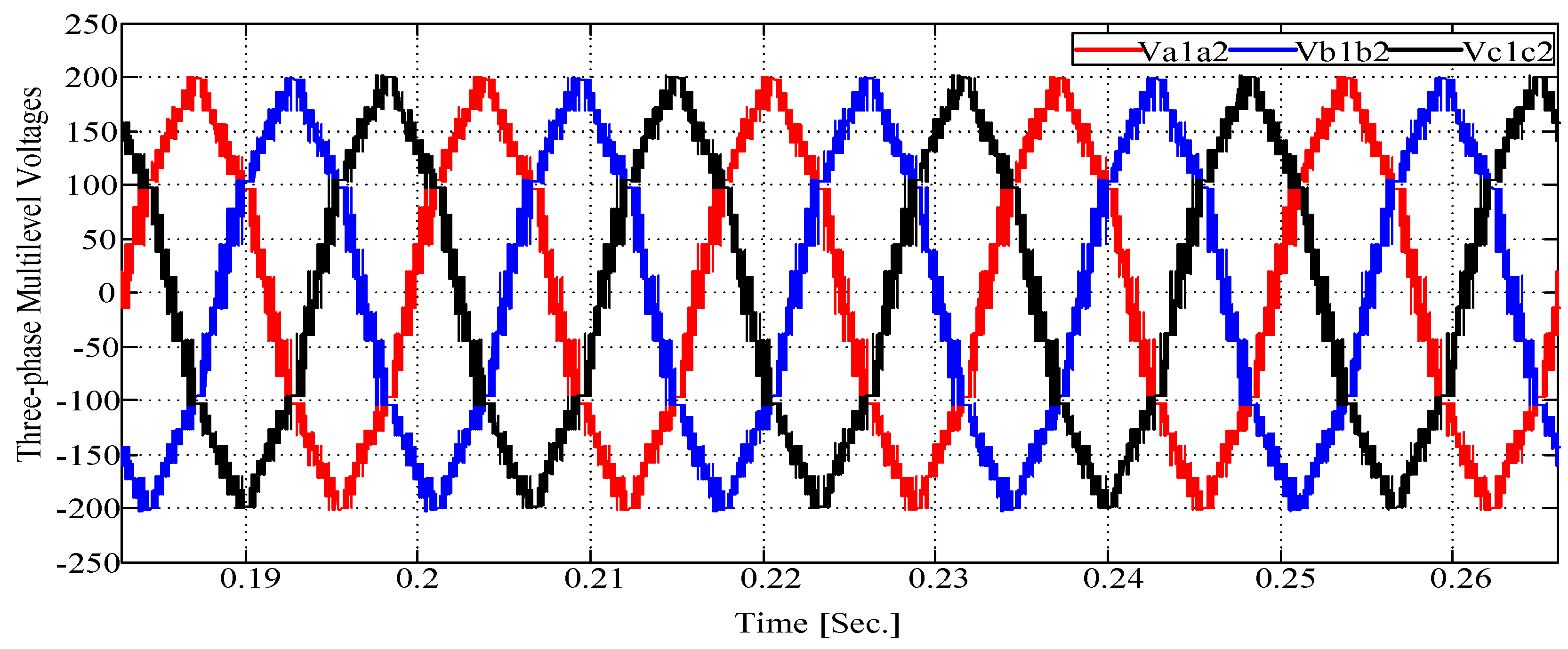
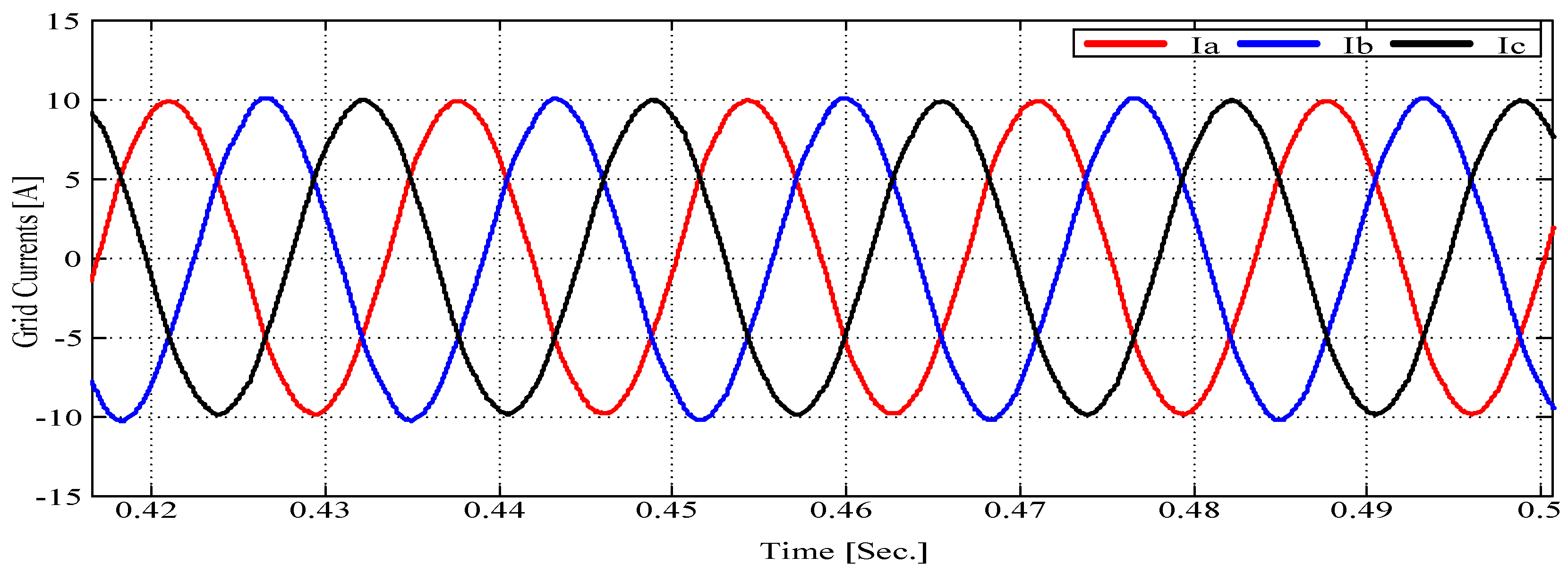
The generated three-phase voltages were measured across the primary windings of the transformers , , and . The number of voltage steps produced from the proposed MLI was 22, as shown in Figure 7. The three-phase currents injected into the grid can be seen in Figure 8. In addition, the harmonic spectrum of the line current, , is displayed in Figure 9. The total harmonic distortion (THD) of the grid current, , was 2.22%, which was less than the IEEE-519 standard limit of 5%.
The THD can be calculated according to the following equation:
where h is the harmonic order, is the RMS value of the current at h order, and is the RMS value of the fundamental current.
As seen in Figure 9, the first harmonic bands appear with an amplitude of 0.2% at two times the fundamental frequency. Then the third, fifth, and seventh harmonic orders appear with amplitudes of 0.3%, 1.6%, and 1.5%, respectively.
- B.
- Active-Power-Filter Application Case
The closed-loop control scheme shown in Figure 5 is used for APF applications. In this case, the harmonic current term in Equation (2) will be included to be compensated by the proposed MLI. The PV module parameters are shown in Table 2, while the system parameters are seen in Table 3. As discussed in the previous section, the proposed control scheme can be used for APFs only or it is able to work as an APF and integrate the PVs into the grid at the same time. These two scenarios are investigated.
Scenario 1: The control scheme is able to work as an APF only:
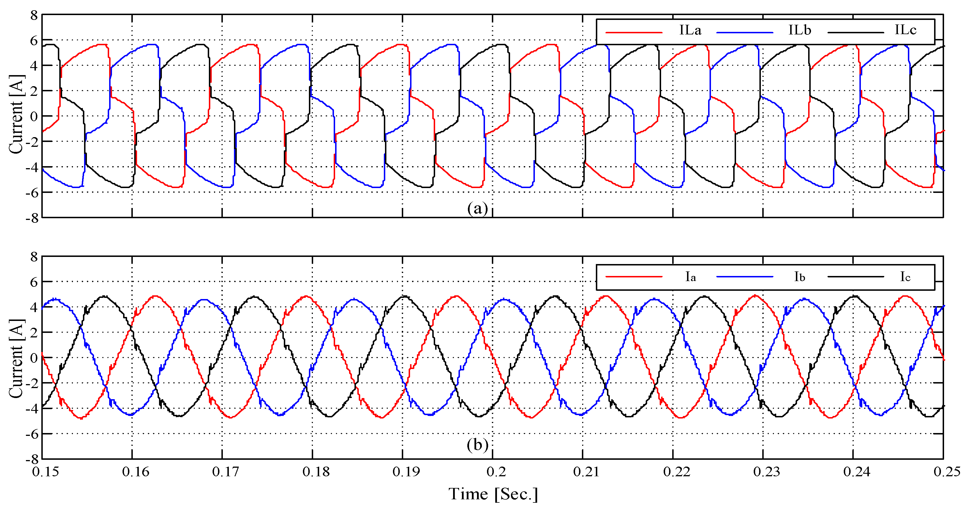
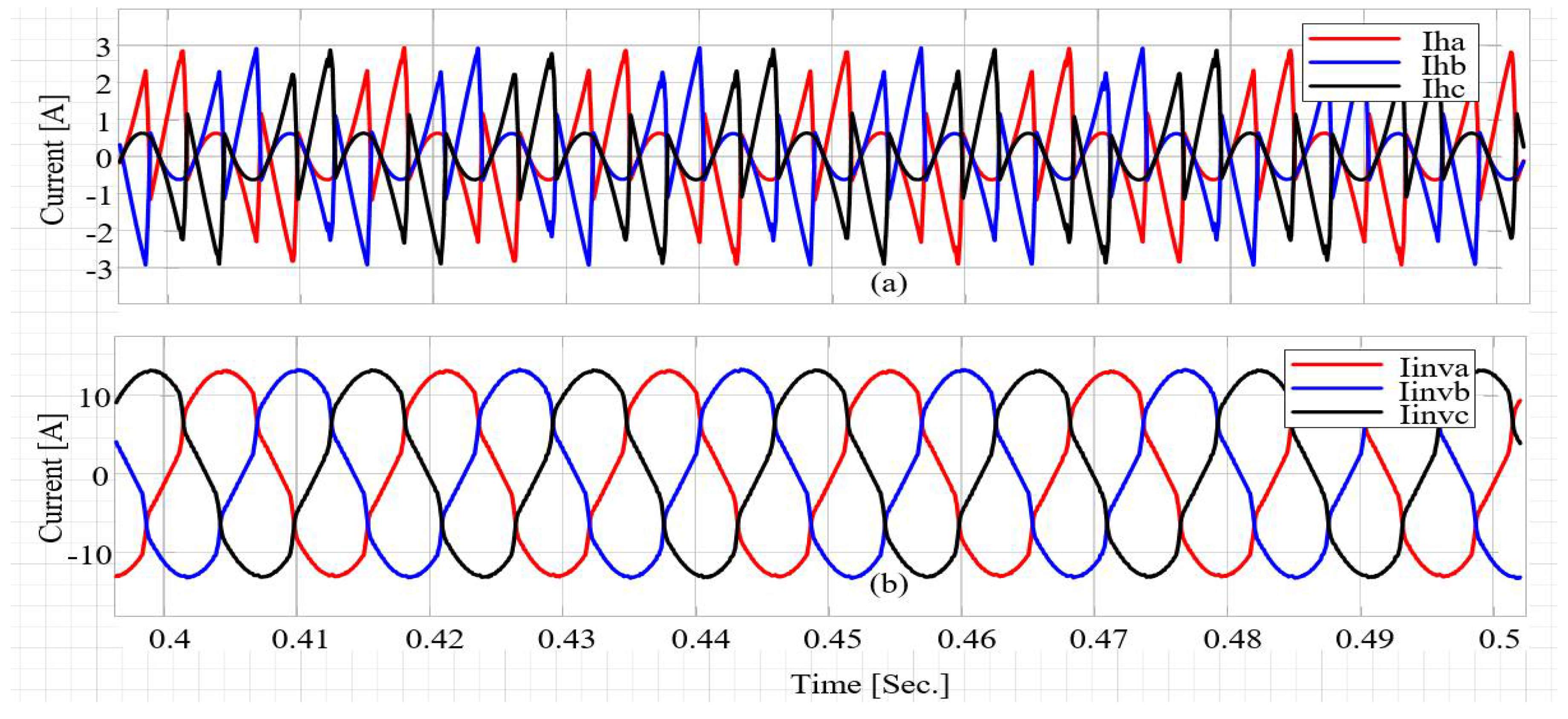
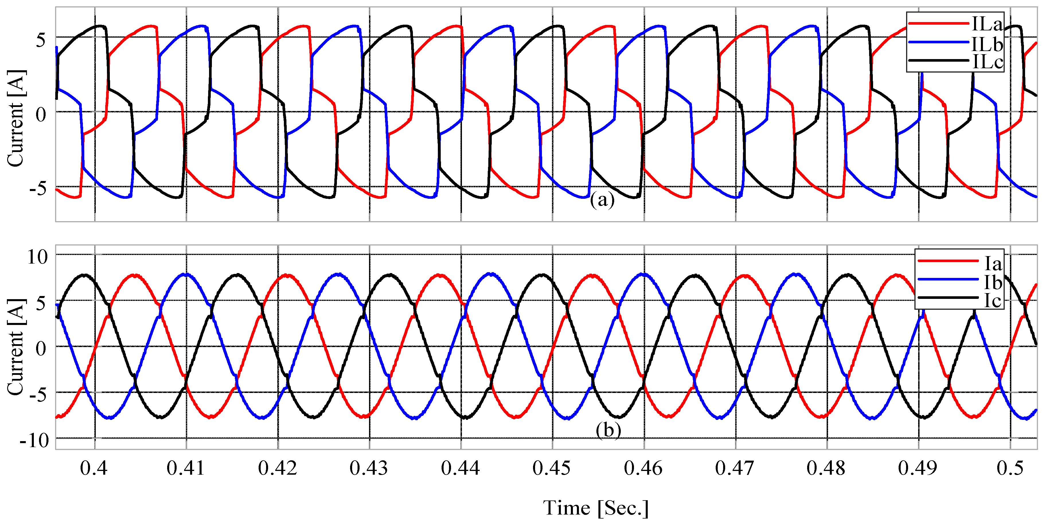
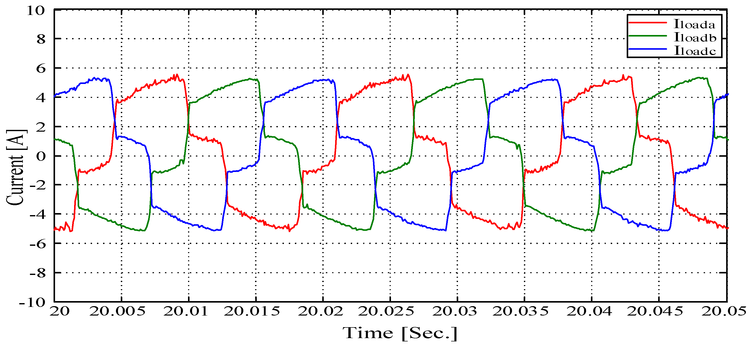
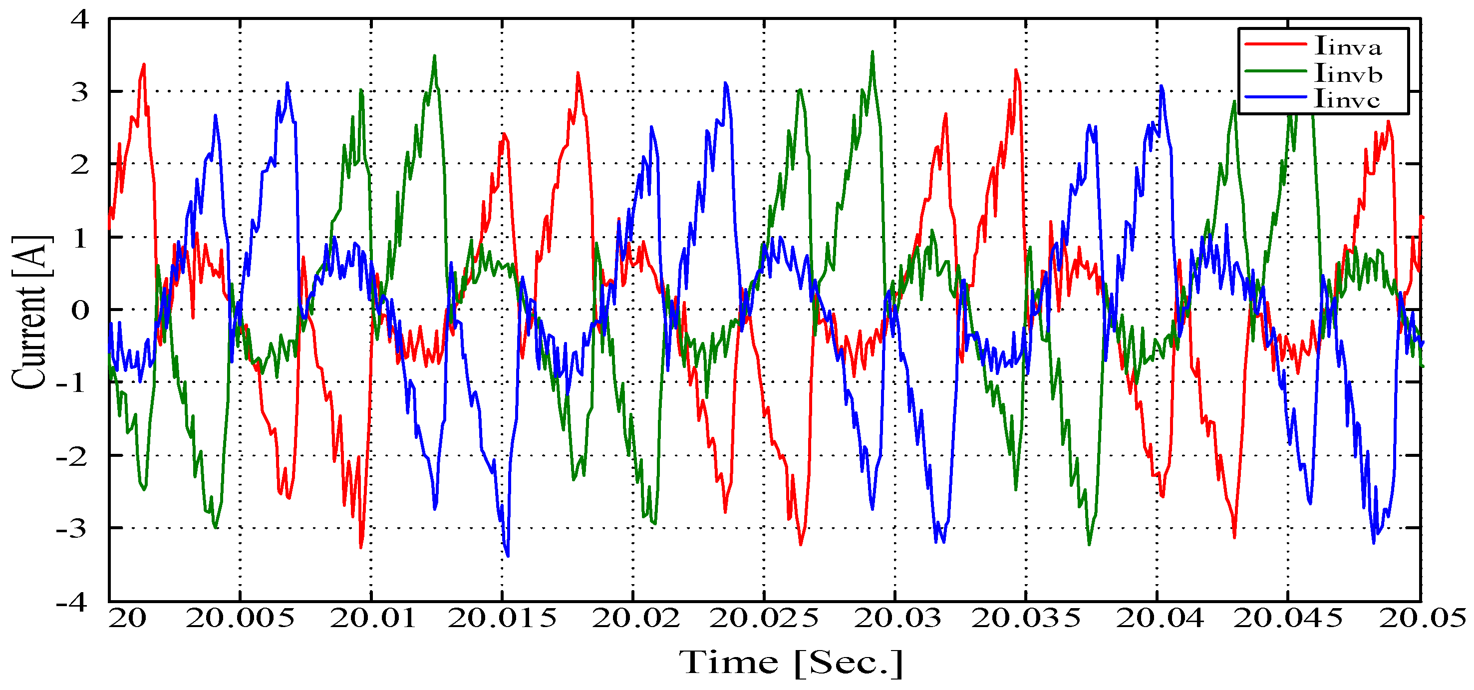
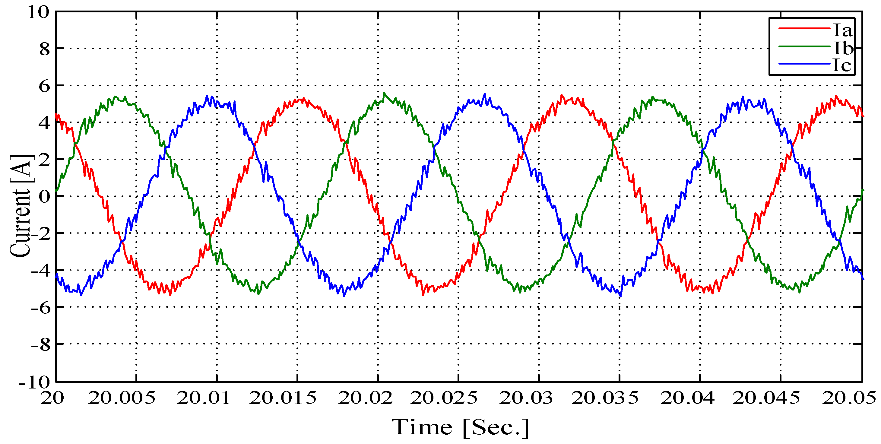
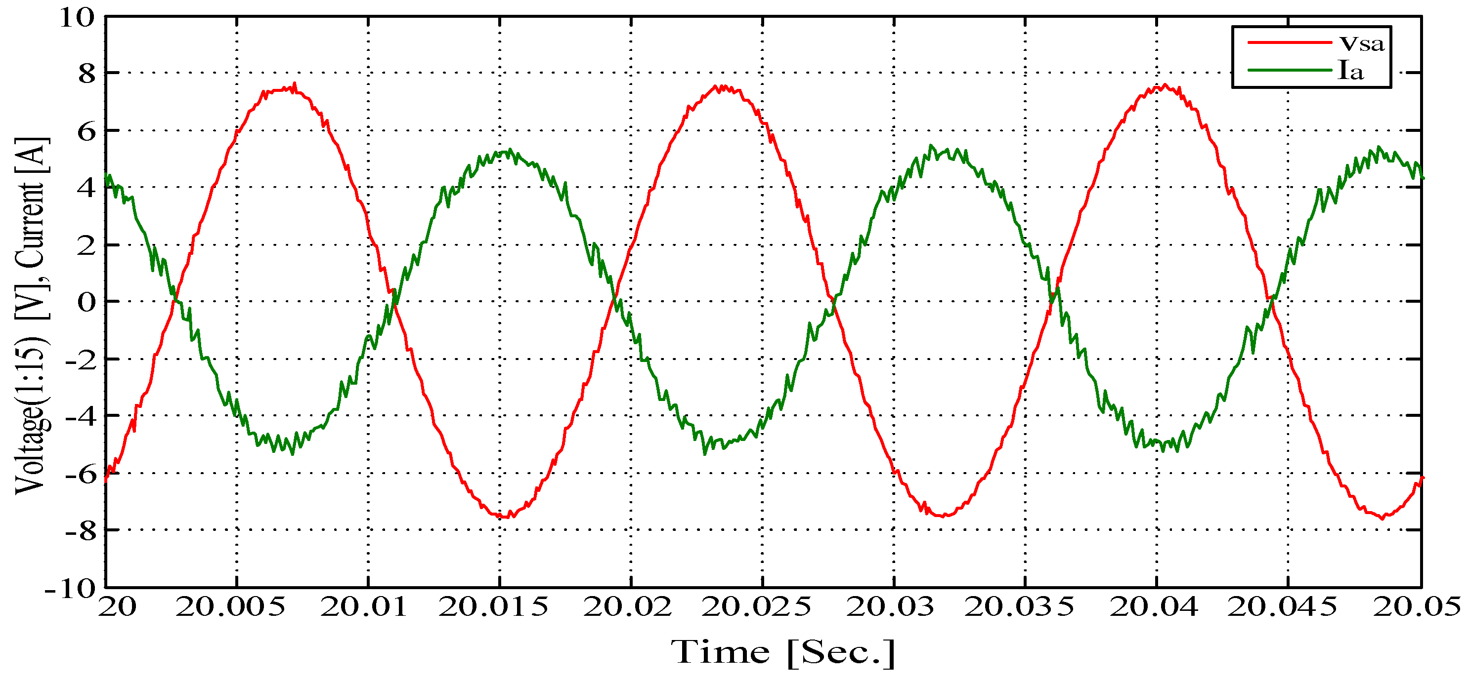
In this scenario, the grid is responsible for supplying the balanced three-phase currents to the nonlinear load, and the proposed MLI is controlled to only compensate for the harmonic currents of the load. The values of the nonlinear load parameters were (, ). To allow the grid to supply the active power to the load, the duty cycle of the DC–DC converter was kept constant at 0.3 (no MPPT was used). The DC-link voltages were regulated to 40 V. Table 3 presents the system parameters that were considered during the simulation. The nonlinear load currents can be seen in Figure 10a, while the three-phase low harmonized grid currents can be seen in Figure 10b. It should be noted that the grid current flowed from the grid to the nonlinear load. As revealed in Figure 10b, the grid currents were balanced, and the nonlinear load did not affect the grid currents. On the other hand, the harmonic currents extracted from the nonlinear load currents can be seen in Figure 11a. These currents were the reference currents of the proposed MLI. As revealed in Figure 11b, the MLI currents followed the extracted harmonic currents of the nonlinear load. Figure 12 shows that the control scheme was successful in maintaining the power-factor unity. The grid currents are shown out of phase with the grid voltages because the grid current direction was from the grid to the load.
Scenario 2: The control scheme is able to work as an APF and integrate the PVs into the grid at the same time.
In this scenario, 24 PV modules were used to guarantee that the inverter supplies the nonlinear load currents and at the same time inject currents into the grid. Twelve PV modules were connected to the upper part of the proposed MLI such that two parallel PV modules were connected to each H-bridge cell. On the other hand, the other 12 PV modules were connected to the lower part of the MLI such that four parallel PV modules were connected to each VSI unit. The proposed control scheme will generate the reference inverter currents that equal the grid current and the nonlinear load currents. The MLI will supply the distorted nonlinear load currents and at the same time will inject currents into the grid with low distortion.
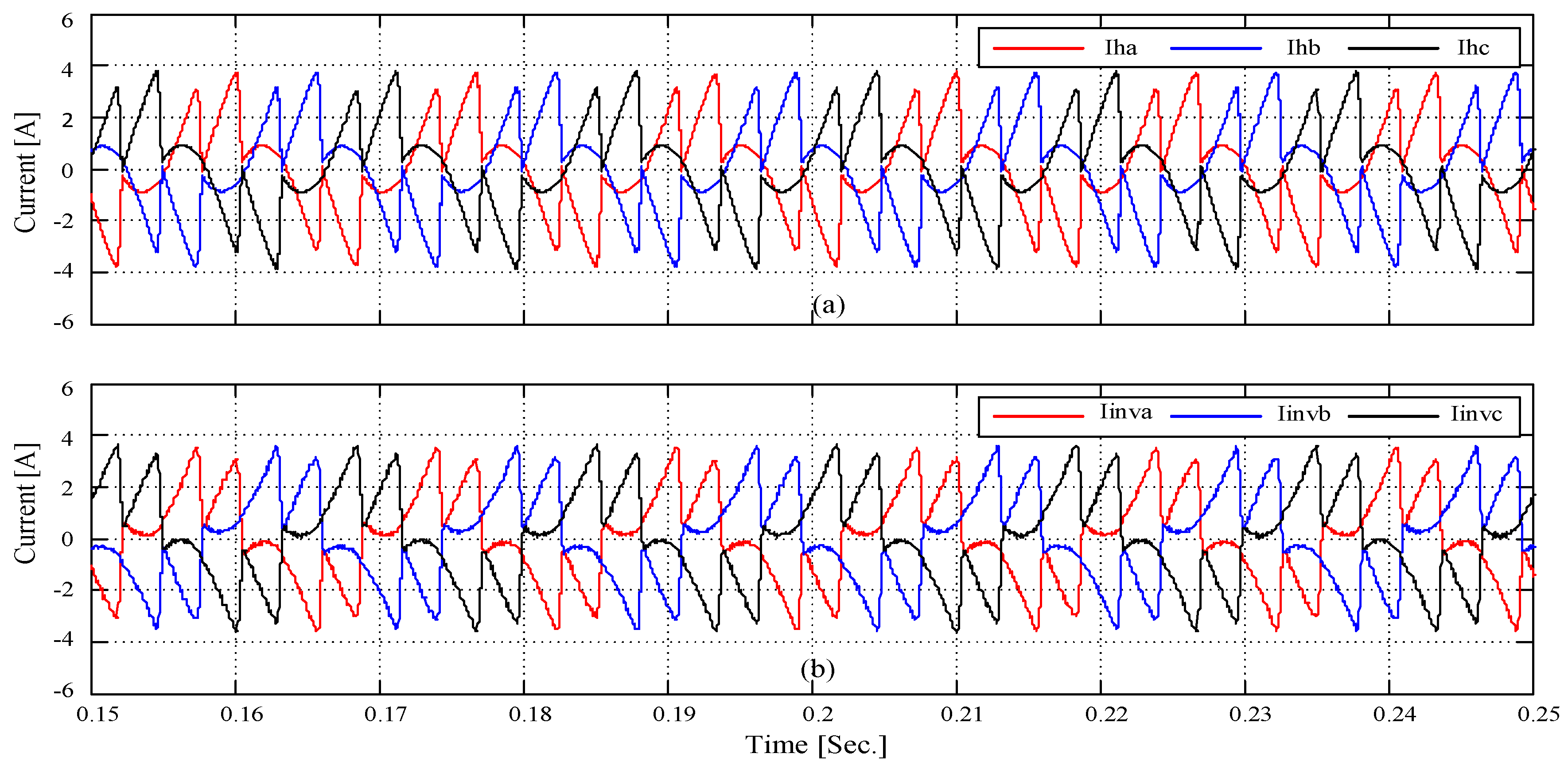
Figure 13a shows the extracted harmonic currents of the nonlinear load. In addition, the actual MLI currents are seen in Figure 13b. As can be seen, the inverter currents were not a mirror to the load harmonic load current. The inverter currents contained the nonlinear load currents and the injected currents to the grid. Moreover, Figure 14a shows the nonlinear load currents while Figure 14b shows the grid currents.
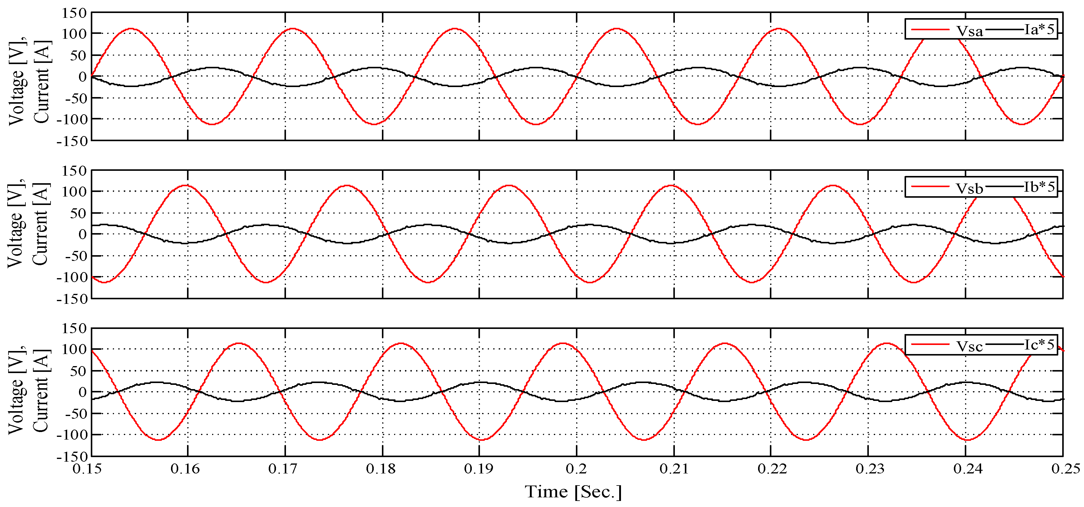
As can be seen, the proposed control scheme succeeded in keeping the grid current in phase with the grid voltage, so that the power factor was kept unity, as seen in Figure 15.
4. Experimental Results
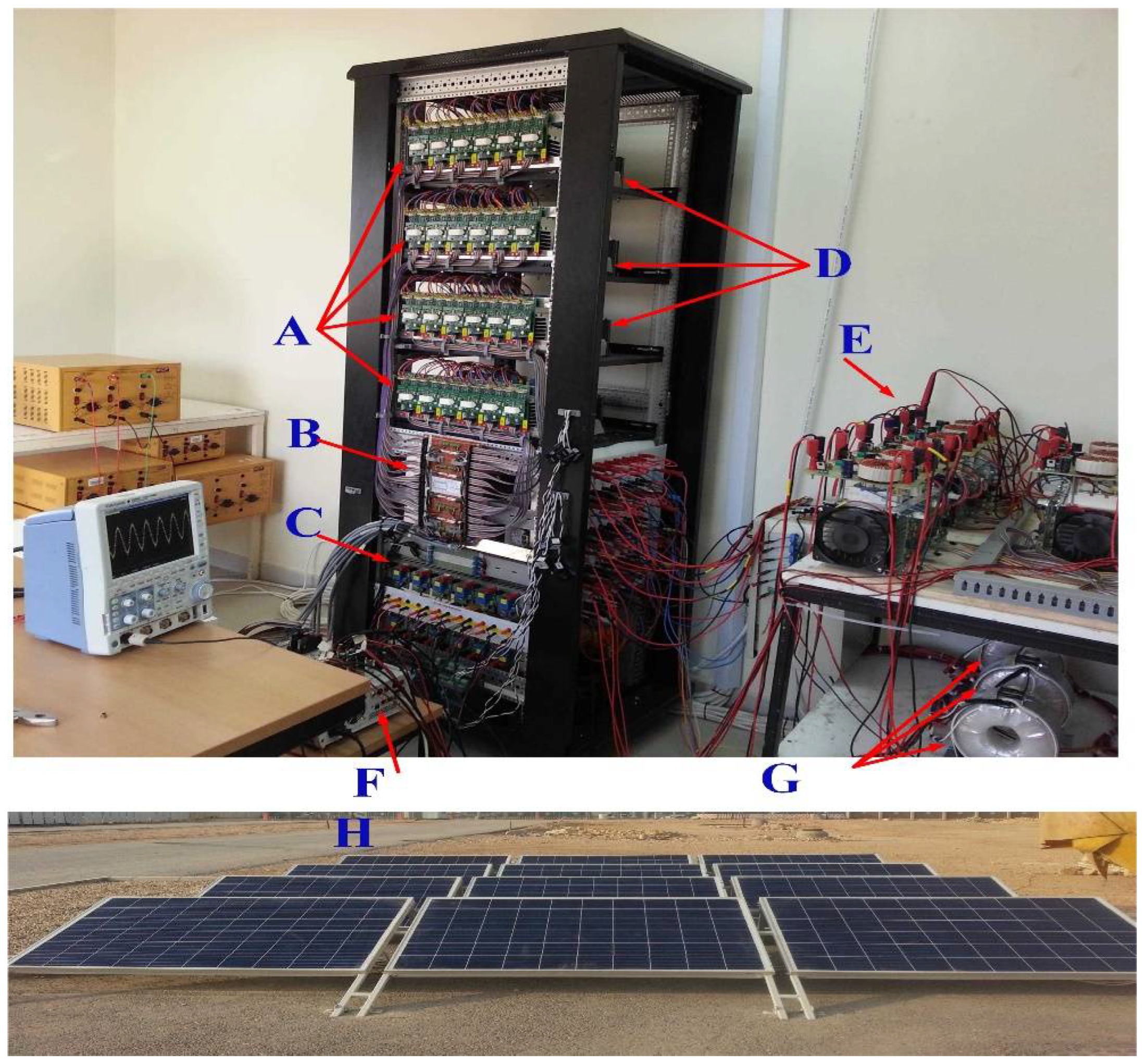
The proposed MLI was built in the lab and tested for PV–grid connections as well as for APF applications. The hardware setup of the proposed MLI is seen in Figure 16. The PV module parameters are seen in Table 2. The closed-loop control scheme explained in Section 3 was used to perform the closed-loop control of the proposed system. The PWM pulses that were generated were transferred to the IGBTs through the use of a DS1202 board. Two cases were performed, PV-grid connections and APF applications, as seen in the simulation section. The same two cases were experimentally implemented.
- A.
- Grid-Connected PV Application Case
A 4.2 mH interface inductor was used to establish the connection between the proposed topology and the grid during experimental testing. The parameters used for the experiment can be seen in Table 1. The entire closed-loop control scheme depicted in Figure 3 and Figure 4 was used to execute the constructed inverter. In this case, the nonlinear load was disconnected from the constructed inverter; therefore, the harmonic current extraction term from (2) was zero. In addition, the reactive current reference of the constructed inverter was set to zero to guarantee unity-power factor. The proposed topology was used only to connect the PV modules to the grid. Twelve PV modules were used in the experimental setup; six of them are connected to the upper part such that one PV module was assigned for each H-bridge cell and the other six PV modules were connected to the lower part such that two parallel PV modules were assigned to each VSI unit. The P&O MPPT algorithm was used to track the maximum power of the PV modules by using a DC–DC Ćuk converter.
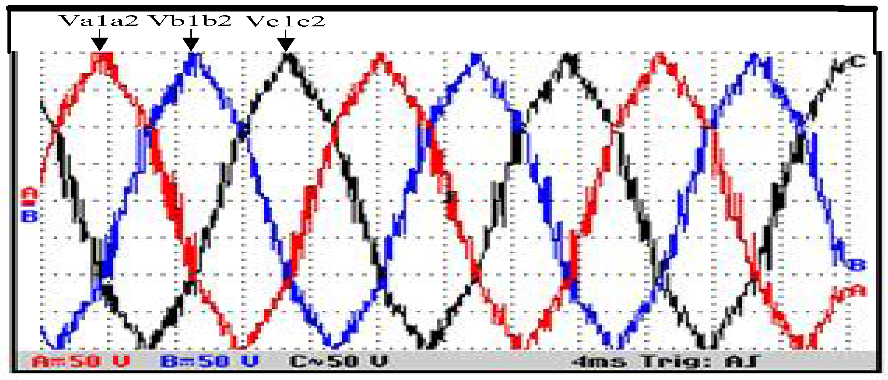
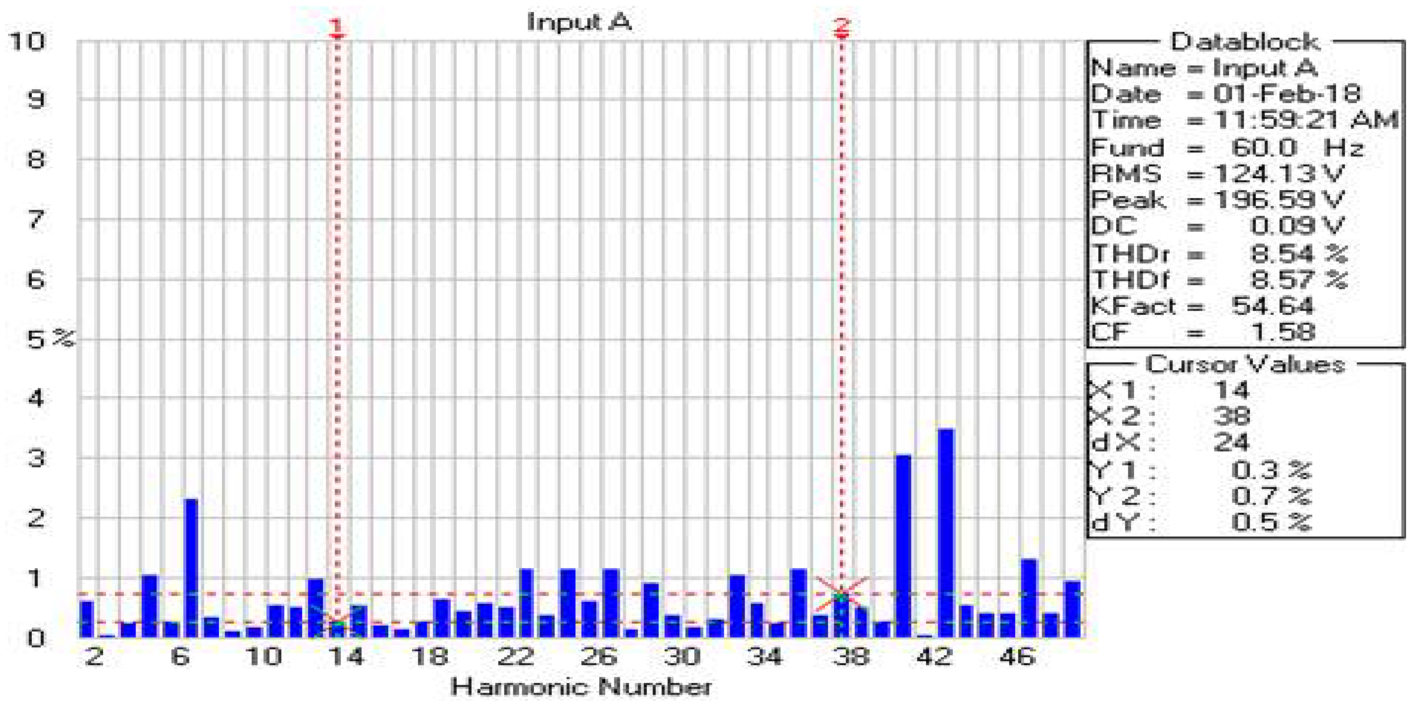
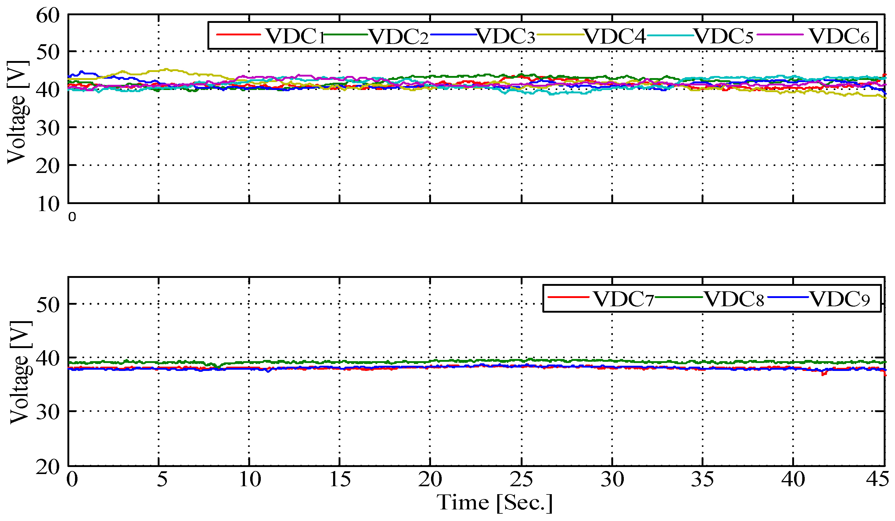
Figure 17 shows the experimental DC-link voltages of the proposed topology. This figure demonstrates that the control scheme was successful in maintaining the DC-link voltages at the reference voltages. On the other hand, the three-phase grid voltages were measured using voltage sensor model LV 25-P to be used for the phase-locked loop. A snapshot of the generated voltages (,, across the primary windings of the , , and transformers) measured via an oscilloscope is shown in Figure 18. Figure 19 reveals the harmonic spectrum of the generated voltage . As displayed in this figure, the THD was 8.57%. Figure 20 shows the grid currents measured by the Hall-effect current sensor model LTS 25-NP.
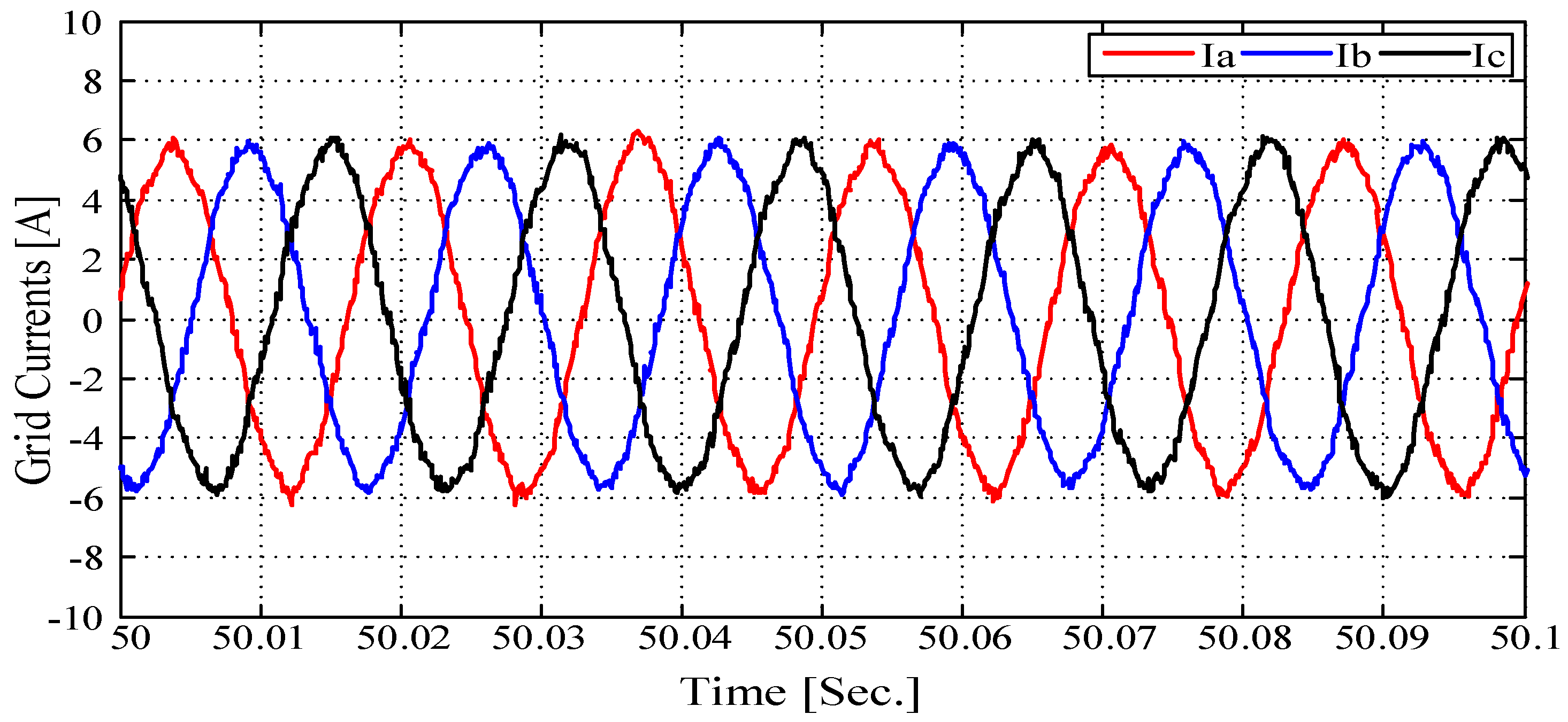
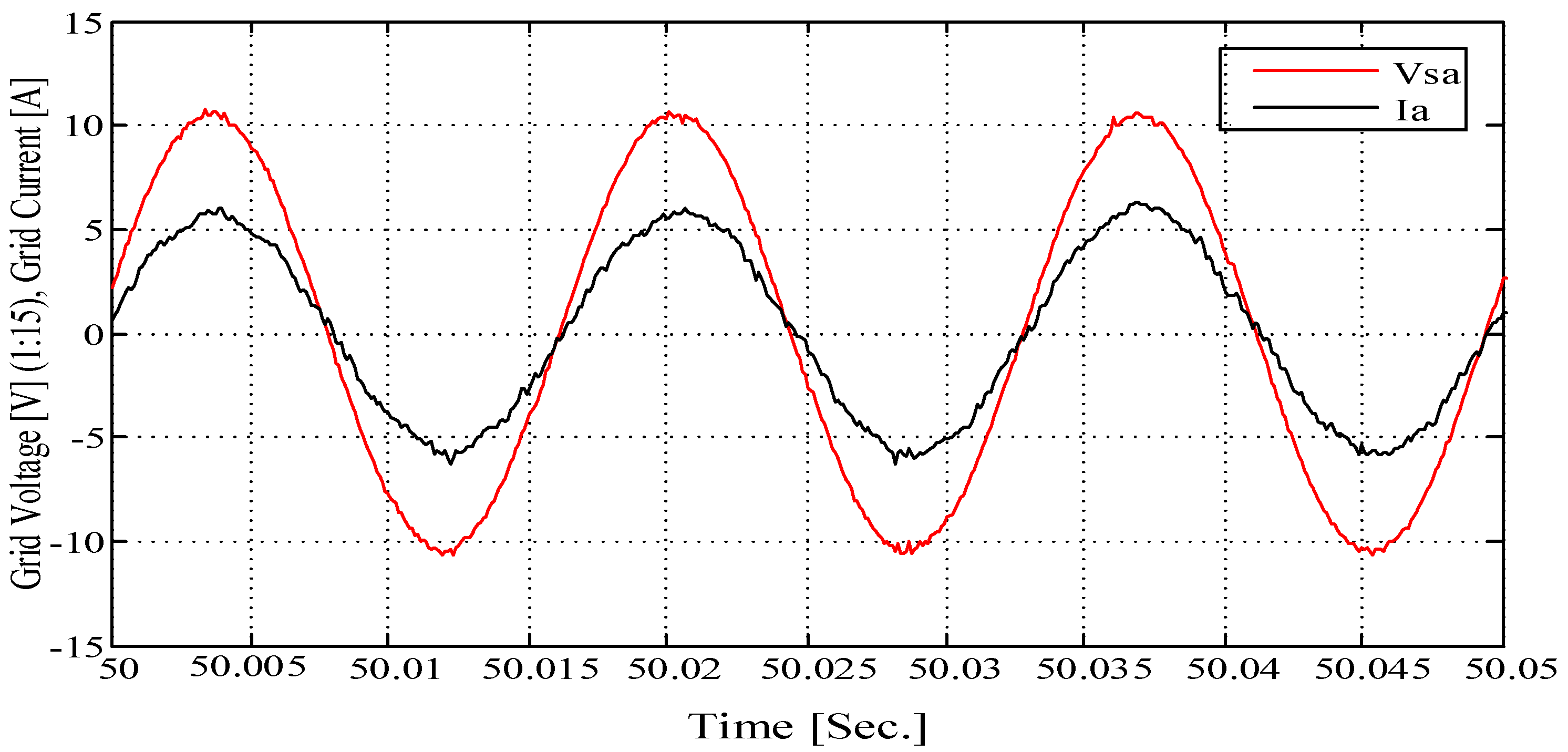
The proposed control scheme succeeded in keeping the grid currents in phase with the grid voltages so that the power factor was unified, as demonstrated in Figure 21. From another point of view, the THD of the grid current,, was 4.41%, which is within the IEEE-519 standard limit. The harmonic spectrum of the grid current in the proposed MLI can be seen in Figure 22.
- B.
- APF-Application Case
In this case, the constructed inverter was experimentally used for APF application. That is, the control scheme was able to work as an APF only. The parameters used for the experiment can be seen in Table 3. In addition, the harmonic current term in Equation (2) was be included so as to be compensated by the MLI. The resulting PWM pulses were then sent to the IGBTs via the DS1202 board. The constructed MLI was controlled to only compensate the harmonic contents of the load currents, while the grid supplied the three-phase positive-sequence currents of the nonlinear load.
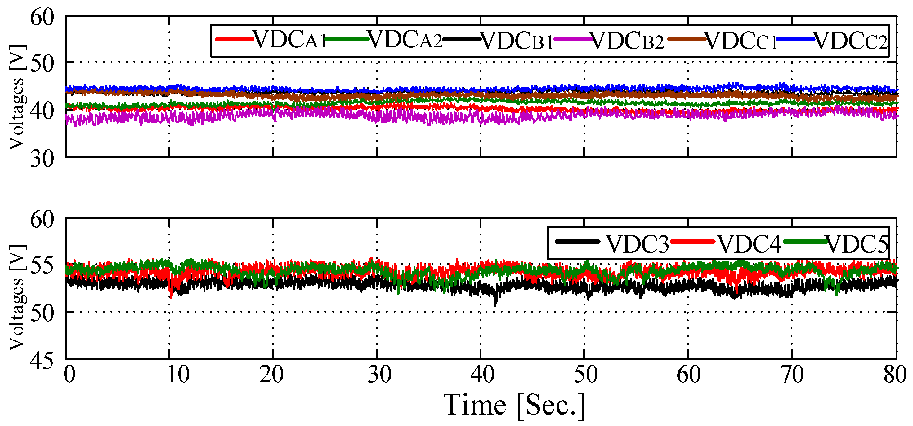
The values of the nonlinear load parameters were ,. To allow the grid to feed power to the nonlinear load, the duty cycle of the DC-DC converter was kept constant at 0.3 (no MPPT is used). The DC-link controllers were successful in maintaining the DC-link voltages at reference levels, as seen in Figure 23. These voltages were measured via analog-to-digital converters by using voltage sensors and plotted in the control desk of the MicroLabBox.
On the other hand, Figure 24 shows the experimental load currents measured by using Hall-effect current sensors. As seen in Figure 24, the load currents are not sine waves since they are highly distorted due to the nonlinear loads. As explained in the control scheme, the harmonic currents of the load were extracted from the load current so as to be compensated by the inverter. The experimental extracted harmonic load currents (the experimental currents of APF) are shown in Figure 25.
These harmonic currents were then used as a reference for the inverter currents so that the inverter compensated only these load current harmonics, and the grid supplied the nonharmonic currents. The experimental three-phase grid currents are shown in Figure 26.
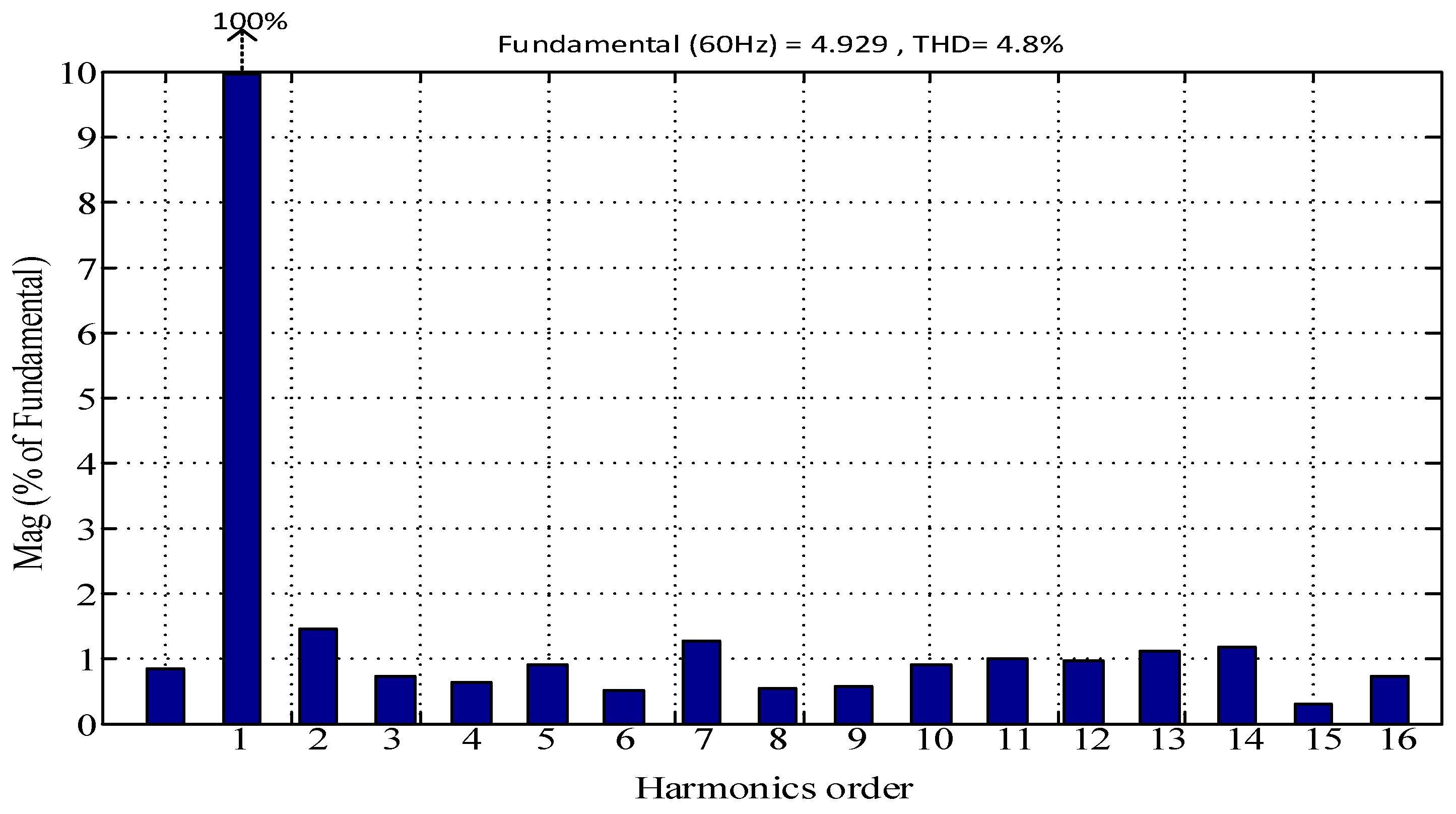
The line currents and the grid voltages were out of phase, as revealed in Figure 27, so that the power factor was kept unified. The out-of-phase grid currents were due to the current sensors measuring the current from the grid to the load. On the other hand, the THD of the line currents was 4.8%, which had acceptable harmonic content of less than 5%, as defined by the IEEE-519 standard. The harmonic spectrum of the grid current, , is shown in Figure 28.
5. Conclusions
A three-phase hybrid cascaded MLI configuration for APF applications has been proposed in this paper. The proposed configuration conjoins the cascaded H-bridge MLI configuration and the three-phase cascaded VSI configuration via OEWs. This topology uses fewer switches than typical MLI topologies while improving the voltage levels of the proposed MLI. Twenty-two voltage levels are generated per phase from this topology by using only 42 switches. Table 4 shows a comparison of the proposed topologies with the conventional MLI topologies to produce 21 voltage levels (one level lower than the number of levels generated by the proposed topology). The proposed topologies have fewer switches than the prior art MLI topologies. The modularity of the proposed topologies is higher and the proposed topologies have fewer DC-link capacitors than other MLI topologies. For a comparison of conduction, the voltage and current stresses of the other topologies were then compared using the same number of switches as in the proposed topology. A control scheme was proposed to execute the proposed topology for APF application. The proposed MLI-based APF was used to compensate the harmonic load currents while the grid supplied the fundamental positive-sequence currents of the load. The proposed APF topology was simulated by using the SIMULINK environment. The nonlinear load was implemented by using a three-phase diode bridge circuit connected to the resistive inductive loads. To validate the good performance of the proposed MLI and the accuracy of the control, the MLI was built in a lab, and the generated switching pulses were implemented on the MicroLabBox data acquisition system and fired into the IGBTs through gate drives. The proposed topology and its related proposed control scheme were experimentally tested for the use for a PV–grid connection and for APF applications. The simulation and the experimental results show that the proposed APF is functions well in eliminating the unwanted harmonics generated by the nonlinear load. The THD of the line currents was within the acceptable limits as defined by IEEE-519 standard.
Author Contributions
Conceptualization, A.M.N. and A.A.A.-S.; Data curation, A.M.N. and A.A.; Formal analysis, A.M.N. and A.A.A.-S.; Funding acquisition, A.M.N. and A.A.; Investigation, A.A.A.-S. and K.E.A.; Methodology, A.M.N. and A.A.A.-S.; Project administration, A.A. and K.E.A.; Software, A.M.N., A.A., A.A.A.-S. and K.E.A.; Supervision, A.A. and K.E.A.; Writing—original draft, A.M.N. and A.A.A.-S.; Writing—review & editing, A.M.N. and A.A. All authors have read and agreed to the published version of the manuscript.
Funding
This research received no external funding.
Informed Consent Statement
Not applicable.
Acknowledgments
This work was supported by the National Plan for Science, Technology, and Innovation, King Abdulaziz City for Science and Technology, Kingdom of Saudi Arabia, Award Number (13-ENE1157-02).
Conflicts of Interest
The authors declare no conflict of interest.
References
- Choudhury, S.; Bajaj, M.; Dash, T.; Kamel, S.; Jurado, F.J.E. Multilevel Inverter: A Survey on Classical and Advanced Topologies, Control Schemes, Applications to Power System and Future Prospects. Energies 2021, 14, 5773. [Google Scholar] [CrossRef]
- Al-Shammáa, A.A.; Noman, A.M.; Addoweesh, K.E.; Alabduljabbar, A.A.; Alolah, A.I. Multilevel Converter by Cascading Two-Level Three-Phase Voltage Source Converter. Energies 2018, 11, 843. [Google Scholar] [CrossRef]
- Galván, L.; Gómez, P.J.; Galván, E.; Carrasco, J.M.J.E. Optimization-Based Capacitor Balancing Method with Customizable Switching Reduction for CHB Converters. Energies 2022, 15, 1976. [Google Scholar] [CrossRef]
- Marzoughi, A.; Burgos, R.; Boroyevich, D.; Xue, Y. Investigation and comparison of cascaded H-bridge and modular multilevel converter topologies for medium-voltage drive application. In Proceedings of the 40th Annual Conference of the IEEE Industrial Electronics Society-IECON, Dallas, TX, USA, 29 October–1 November 2014; pp. 1562–1568. [Google Scholar]
- Espinosa, E.; Melín, P.; Baier, C.; Espinoza, J.; Garcés, H.J.E. An Efficiency Analysis of 27 Level Single-Phase Asymmetric Inverter without Regeneration. Energies 2021, 14, 1459. [Google Scholar] [CrossRef]
- Chattopadhyay, S.K.; Chakraborty, C. Performance of three-phase asymmetric cascaded bridge (16: 4: 1) multilevel inverter. IEEE Trans. Ind. Electron. 2015, 62, 5983–5992. [Google Scholar] [CrossRef]
- Sivakumar, K.; Das, A.; Ramchand, R.; Patel, C.; Gopakumar, K. A hybrid multilevel inverter topology for an open-end winding induction-motor drive using two-level inverters in series with a capacitor-fed H-bridge cell. IEEE Trans. Ind. Electron. 2010, 57, 3707–3714. [Google Scholar] [CrossRef]
- Rajeevan, P.; Sivakumar, K.; Patel, C.; Ramchand, R.; Gopakumar, K. A seven-level inverter topology for induction motor drive using two-level inverters and floating capacitor fed H-bridges. IEEE Trans. Power Electron. 2011, 26, 1733–1740. [Google Scholar] [CrossRef]
- Das, S.R.; Ray, P.K.; Sahoo, A.K.; Ramasubbareddy, S.; Babu, T.S.; Kumar, N.M.; Elavarasan, R.M.; Mihet-Popa, L. A Comprehensive Survey on Different Control Strategies and Applications of Active Power Filters for Power Quality Improvement. Energies 2021, 14, 4589. [Google Scholar] [CrossRef]
- Lumbreras, D.; Gálvez, E.; Collado, A.; Zaragoza, J.J.E. Trends in power quality, harmonic mitigation and standards for light and heavy industries: A review. Energies 2020, 13, 5792. [Google Scholar] [CrossRef]
- Urquizo, J.; Singh, P.; Kondrath, N.; Hidalgo-León, R.; Soriano, G. Using D-FACTS in microgrids for power quality improvement: A review. In Proceedings of the IEEE Second Ecuador Technical Chapters Meeting (ETCM), Salinas, Ecuador, 16–20 October 2017; pp. 1–6. [Google Scholar]
- Rachmildha, T.D. Optimized Combined System of Shunt Active Power Filters and Capacitor Banks. Int. J. Electr. Eng. Inform. 2011, 3, 326–335. [Google Scholar] [CrossRef]
- Bag, A.; Subudhi, B.; Ray, P.K. Comparative analysis of sliding mode controller and hysteresis controller for active power filtering in a grid connected PV system. Int. J. Emerg. Electr. Power Syst. 2018, 19, 1–13. [Google Scholar] [CrossRef]
- Pou, J.; Boroyevich, D.; Pindado, R. Effects of imbalances and nonlinear loads on the voltage balance of a neutral-point-clamped inverter. IEEE Trans. Power Electron. 2005, 20, 123–131. [Google Scholar] [CrossRef]
- Liu, Q.; Li, Y.; Hu, S.; Luo, L. A transformer integrated filtering system for power quality improvement of industrial DC supply system. IEEE Trans. Ind. Electron. 2019, 67, 3329–3339. [Google Scholar] [CrossRef]
- Liu, Q.; Li, Y.; Hu, S.; Luo, L.; Systems, E. A controllable inductive power filtering system: Modeling, analysis and control design. Int. J. Electr. Power Energy Syst. 2019, 105, 717–728. [Google Scholar] [CrossRef]
- Ali, H.H.; Kamal, N.A.; Elbasuony, G.S. Two-Level Grid-Side Converter-Based STATCOM and Shunt Active Power Filter of Variable-Speed DFIG Wind Turbine-Based WECS Using SVM for Terminal Voltage. Int. J. Serv. Sci. Manag. Eng. Technol. (IJSSMET) 2021, 12, 169–202. [Google Scholar]
- Jignesh, P.; Jadeja, R.; Trivedi, T. Cascaded Three Level Inverter Based Shunt Active Power Filter with Modified Three Level Hysteresis Current Control. Int. Rev. Model. Simul. 2018, 11, 125–197. [Google Scholar]
- Sihem, G.; Azar, A.T.; Dib, D. Three-level (NPC) shunt active power filter based on fuzzy logic and fractional-order PI controller. Int. J. Autom. Control. 2021, 15, 149–169. [Google Scholar]
- Dawid, B.; Jarek, G.; Michalak, J.; Zygmanowski, M. Control method of four wire active power filter based on three-phase neutral point clamped T-type converter. Energies 2021, 14, 8427. [Google Scholar]
- Salim, C.H.E.N.N.A.I. Shunt Active Power Filter Performances based on Seven-level NPC Inverter using Fuzzy and LS-PWM Control Scheme. Electroteh. Electron. Autom. 2022, 1, 23–30. [Google Scholar]
- Adrikowski, T.; Bula, D.; Pasko, M. Three-phase active power filter with T-NPC type inverter. In Proceedings of the 2018 Progress in Applied Electrical Engineering (PAEE), Koscielisko, Poland, 18–22 June 2018; pp. 1–5. [Google Scholar]
- Escobar, G.; Martinez-Rodriguez, P.R.; Iturriaga-Medina, S.; Vazquez-Guzman, G.; Sosa-Zuñiga, J.M.; Langarica-Cordoba, D. Control Design and Experimental Validation of a HB-NPC as a Shunt Active Power Filter. Energies 2020, 13, 1691. [Google Scholar] [CrossRef]
- Soumyadeep, R.; Gupta, N.; Gupta, R.A. A novel non-linear control for three-phase five-level cascaded H-bridge inverter based shunt active power filter. Int. J. Emerg. Electr. Power Syst. 2018, 19, 1–11. [Google Scholar] [CrossRef]
- Wang, H.; Liu, S. An optimal operation strategy for an active power filter using cascaded H-bridges in delta-connection. Electr. Power Syst. Res. 2019, 175, 105918. [Google Scholar] [CrossRef]
- Sochor, P.; Hirofumi, A. Theoretical and experimental comparison between phase-shifted PWM and level-shifted PWM in a modular multilevel SDBC inverter for utility-scale photovoltaic applications. IEEE Trans. Ind. Appl. 2017, 53, 4695–4707. [Google Scholar] [CrossRef]
- Nair, V.; Gopakumar, K.; Franquelo, L.G. A very high resolution stacked multilevel inverter topology for adjustable speed drives. IEEE Trans. Ind. Electron. 2017, 65, 2049–2056. [Google Scholar] [CrossRef]
- Behrouzian, E.; Bongiorno, M. DC-link voltage modulation for individual capacitor voltage balancing in cascaded H-bridge STATCOM at zero current mode. In Proceedings of the 20th European Conference on Power Electronics and Applications, Riga, Latvia, 17–21 September 2018; pp. 1–10. [Google Scholar]
- Mariem, T.; Guermazi, A.; Ghariani, M. Cascaded Multilevel Inverter for PV-Active Power Filter Combination into the Grid-Tied Solar System. Int. J. Renew. Energy Res. (IJRER) 2020, 10, 1810–1819. [Google Scholar]
- Nageswar, R.B.; Suresh, Y.; Panda, A.K.; Naik, B.S.; Jammala, V. Development of cascaded multilevel inverter based active power filter with reduced transformers. CPSS Trans. Power Electron. Appl. 2020, 5, 147–157. [Google Scholar]
- Noman, A.M.; Al-Shammáa, A.A.; Addoweesh, K.E.; Alabduljabbar, A.A.; Alolah, A.I.J.E. Cascaded multilevel inverter topology based on cascaded H-bridge multilevel inverter. Energies 2018, 11, 895. [Google Scholar] [CrossRef] [Green Version]
- Noman, A.M.A.; Alshammaa, A.A.; Addoweesh, K.E.; Alabduljabbar, A.A.A.; Alolah, A.I. Hybrid CHB-TVSI Multilevel Voltage Source Inverter. U.S. Patent US10141865B1, 2018. [Google Scholar]
- Hamadi, A.; Rahmani, S.; Al-Haddad, K.; Al-Turki, Y.A. A three-phase three wire grid-connect photovoltaic energy source with sepic converter to track the maximum power point. In Proceedings of the 37th Annual Conference of the IEEE Industrial Electronics Society-IECON, Melbourne, VIC, Australia, 7–10 November 2011; pp. 3087–3092. [Google Scholar]
Figure 1.
Proposed APF topology. Upper part: This part is the conventional cascaded H-bridge MLI which consists of three-phase systems. Each phase consists of N H-bridge cells that are cascaded as shown in the stage 1 of Figure 1 such that the terminal of H-bridge cell 1 in phase a, for example, is connected to the terminal of the next H-bridge cell. In addition, the terminal is connected to the terminal of the last H-bridge cell. The same idea is applied to phases b and c. Lower part: This part is a three-phase triple-voltage source inverter, which is made up of three VSIs. Each unit is a three-leg, two-level inverter, and the three units are linked together in a chain, as shown in the lower part of Figure 1. The three VSIs are cascaded with one another by using open-end winding transformers. Finally: The upper part and the lower part are connected to each other via open-end windings. The terminals , , and of stage 1 are connected together to a common point NN. The terminals , , and of the upper part are connected to the points , and of the open-end windings transformers, respectively. The three points , , and of the lower part are connected to the points , , and of the open-end windings transformers, respectively. The secondary sides of the transformer are connected in Y connection and the terminals are connected to the grid and to the nonlinear loads.

Figure 2.
Extraction of the load harmonic currents.

Figure 3.
Proposed voltage control scheme.

Figure 4.
The current controllers. is the reference DC voltage.

Figure 5.
The proposed control scheme for APF application.

Figure 6.
Phase-shifted PWM technique.

Figure 7.
The simulated three-phase generating voltage.

Figure 8.
The simulated three-phase grid currents.

Figure 9.
Harmonic spectrum of the phase a grid current.

Figure 10.
The simulated grid currents and the load currents.

Figure 11.
The simulated harmonic load currents and the active power filter currents.

Figure 12.
The simulated grid currents with the grid voltages.

Figure 13.
(a) The extracted harmonic currents of the nonlinear load and (b) the MLI currents.

Figure 14.
(a) The nonlinear load currents and (b) the grid currents.

Figure 15.
The grid current and the grid voltage.

Figure 16.
Hardware setup of the proposed MLI. A: IGBT drives, B: level shifter, C: voltage/current sensors, D: IGBTs and DC-link capacitors, E: CUK converters, F: dSPACE 1102, G: open-end winding transformers, and H: PV modules.
Figure 16.
Hardware setup of the proposed MLI. A: IGBT drives, B: level shifter, C: voltage/current sensors, D: IGBTs and DC-link capacitors, E: CUK converters, F: dSPACE 1102, G: open-end winding transformers, and H: PV modules.

Figure 17.
Experimental DC-link voltages.

Figure 18.
The snapshot of the three-phase generated voltages.

Figure 19.
Experimental harmonic spectrum of the generated voltage .

Figure 20.
Experimental three-phase grid currents.

Figure 21.
Experimental grid voltage and grid currents.

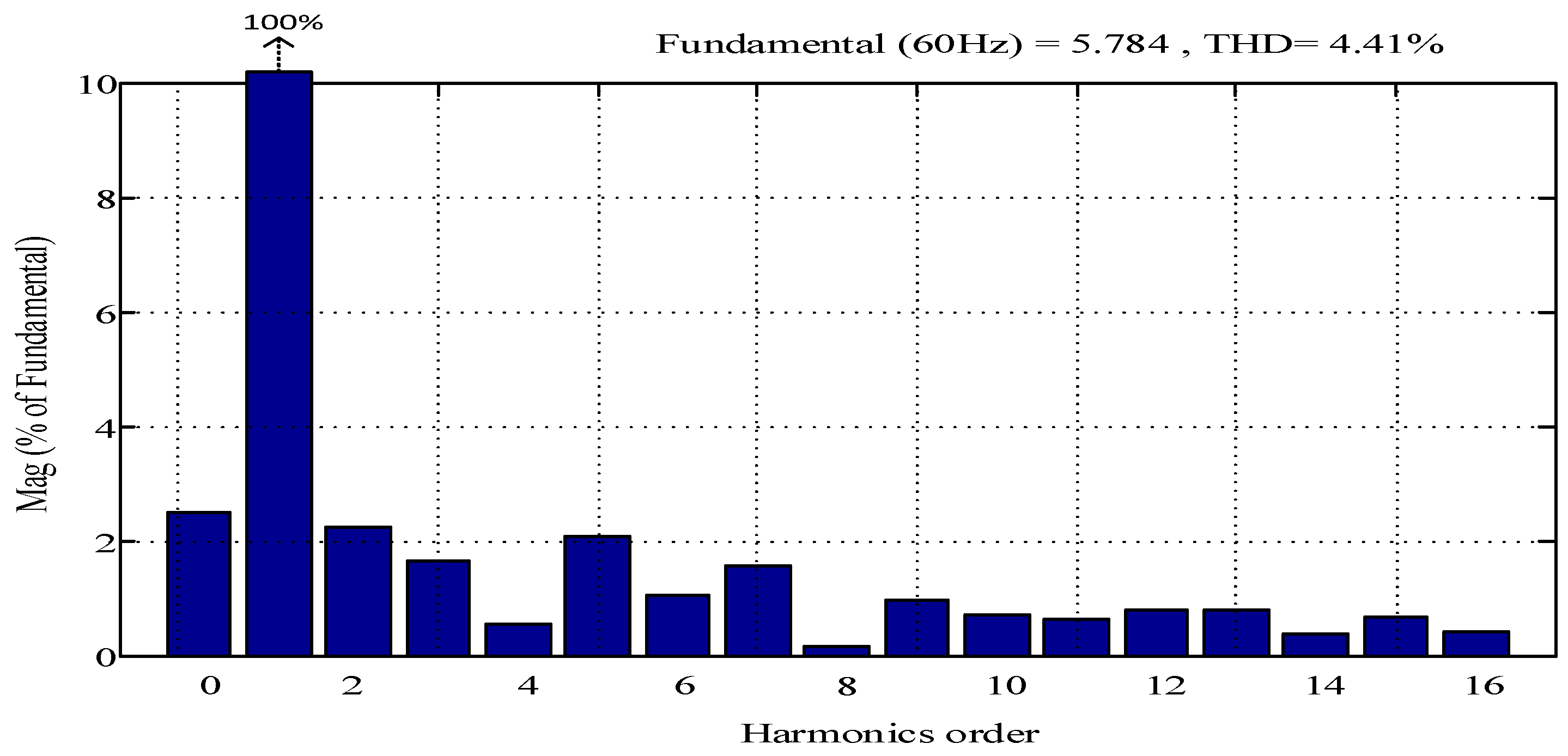
Figure 22.
Experimental harmonic spectrum of the grid current .

Figure 23.
The experimental DC-link voltages.

Figure 24.
The experimental nonlinear load currents.

Figure 25.
The experimental APF currents.

Figure 26.
The experimental three-phase grid currents.

Figure 27.
The experimental grid current and grid voltage.

Figure 28.
Harmonic spectrum of the grid current .


Table 1.
System parameter for simulation and experiment.
| DC-Link Capacitor | 4 mF |
| Interface inductor | 4.2 mH |
| Ćuk switching frequency | 20 kHz |
| Grid-rated RMS voltage | 120 V |
| Reference voltage of each VSI unit (upper part) | 55 V |
| Reference voltage of each H-bridge cell (lower part) | 40 V |
| Inverter switching frequency | 1.5 kHz |
Table 2.
The PV module parameters.
| Maximum Power (Pmax) | 245 W |
| Maximum voltage (Vmax) | 28.8 V |
| Maximum current (Imax) | 8.5 A |
| Open circuit voltage (Voc) | 31.5 V |
| Short circuit current (Isc) | 9.5 A |
Table 3.
System parameter for simulation and experiment (APF application).
| DC-Link Capacitor | 4 mF |
| Connection inductor | 4.2 mH |
| Ćuk switching frequency | 20 KHz |
| Grid-rated RMS voltage | 80 V |
| Reference voltage of each VSI unit (upper part) | 40 V |
| Reference voltage of each H-bridge cell (lower part) | 40 V |
| Inverter switching frequency | 1.5 KHz |
Table 4.
Comparison results.
| NPC | FC | CHB | MMC | Proposed Topology | |
|---|---|---|---|---|---|
| No. of switches | 120 | 120 | 120 | 240 | 42 |
| DC-link capacitors | 20 | 20 | 30 | 60 | 9 |
| No. of inductors | 0 | 0 | 0 | 6 | 3 |
| No. of diodes | 1140 | 0 | 0 | 0 | 0 |
| No. of flying capacitors | 0 | 570 | 0 | 0 | 0 |
| Modularity | No | No | Yes | No | Yes |
| Voltage-balancing problem | Yes | Yes | No | Yes | No |
| Separated DC sources | No | No | Yes | No | Yes |
| Voltage stress | |||||
| Current stress | I | I | I | I | I |
Publisher’s Note: MDPI stays neutral with regard to jurisdictional claims in published maps and institutional affiliations. |
© 2022 by the authors. Licensee MDPI, Basel, Switzerland. This article is an open access article distributed under the terms and conditions of the Creative Commons Attribution (CC BY) license (https://creativecommons.org/licenses/by/4.0/).
Share and Cite
MDPI and ACS Style
Noman, A.M.; Alkuhayli, A.; Al-Shamma’a, A.A.; Addoweesh, K.E. Hybrid MLI Topology Using Open-End Windings for Active Power Filter Applications. Energies 2022, 15, 6434. https://doi.org/10.3390/en15176434
AMA Style
Noman AM, Alkuhayli A, Al-Shamma’a AA, Addoweesh KE. Hybrid MLI Topology Using Open-End Windings for Active Power Filter Applications. Energies. 2022; 15(17):6434. https://doi.org/10.3390/en15176434
Chicago/Turabian StyleNoman, Abdullah M., Abdulaziz Alkuhayli, Abdullrahman A. Al-Shamma’a, and Khaled E. Addoweesh. 2022. "Hybrid MLI Topology Using Open-End Windings for Active Power Filter Applications" Energies 15, no. 17: 6434. https://doi.org/10.3390/en15176434
Note that from the first issue of 2016, this journal uses article numbers instead of page numbers. See further details here.