
Optimization of Fracturing Parameters with Machine-Learning and Evolutionary Algorithm Methods


1
Petroleum Engineering Department, Xi’an Shiyou University, Xi’an 710065, China
2
Research Institute of Petroleum Exploration and Development, PetroChina, Beijing 100083, China
*
Author to whom correspondence should be addressed.
Energies 2022, 15(16), 6063; https://doi.org/10.3390/en15166063
Submission received: 27 June 2022
/
Revised: 4 August 2022
/
Accepted: 4 August 2022
/
Published: 21 August 2022
(This article belongs to the Section F5: Artificial Intelligence and Smart Energy)
Abstract
:Oil production from tight oil reservoirs has become economically feasible because of the combination of horizontal drilling and multistage hydraulic fracturing. Optimal fracture design plays a critical role in successful economical production from a tight oil reservoir. However, many complex parameters such as fracture spacing and fracture half-length make fracturing treatments costly and uncertain. To improve fracture design, it is essential to determine reasonable ranges for these parameters and to evaluate their effects on well performance and economic feasibility. In traditional analytical and numerical simulation methods, many simplifications and assumptions are introduced for artificial fracture characterization and gas percolation mechanisms, and their implementation process remains complicated and computationally inefficient. Most previous studies on big data-driven fracturing parameter optimization have been based on only a single output, such as expected ultimate recovery, and few studies have integrated machine learning with evolutionary algorithms to optimize fracturing parameters based on time-series production prediction and economic objectives. This study proposed a novel approach, combining a data-driven model with evolutionary optimization algorithms to optimize fracturing parameters. We established a significant number of static and dynamic data sets representing the geological and developmental characteristics of tight oil reservoirs from numerical simulation. Four production-prediction models based on machine-learning methods—support vector machine, gradient-boosted decision tree, random forest, and multilayer perception—were constructed as mapping functions between static properties and dynamic production. Then, to optimize the fracturing parameters, the best machine-learning-based production predictive model was coupled with four evolutionary algorithms—genetic algorithm, differential evolution algorithm, simulated annealing algorithm, and particle swarm optimization—to investigate the highest net present value (NPV). The results show that among the four production-prediction models established, multilayer perception (MLP) has the best prediction performance. Among the evolutionary algorithms, particle swarm optimization (PSO) not only has the fastest convergence speed but also the highest net present value. The optimal fracturing parameters for the study area were identified. The hybrid MLP-PSO model represents a robust and convenient method to forecast the time-series production and to optimize fracturing parameters by reducing manual tuning.
1. Introduction
Tight oil resources play a significant role in meeting the ever-growing energy demands of global markets. These reservoirs are complex in nature and have ultra-tight producing formation, so they depend on effective well completion and stimulation treatments for their economic success. In the past decade, both industry and academic researchers have studied tight oil resources intensively and have made tremendous progress, with one acknowledgment being the critical importance of fracture design optimization. However, the industry still struggles to determine the dominant control over tight oil productivity, whether geological or technical. Given certain geological properties, what is the best completion strategy?
To increase production from tight oil reservoirs, optimizing the fracturing parameters is imperative. At present, analytical and numerical simulation methods are applied to comprehensively calculate and evaluate the impact of different fracture sizes and inflow capacities on production. Analytical methods usually do not consider the fracture’s three-dimensional (3D) expansion and cannot predict postfracture capacity [1]. Numerical methods introduce many assumptions and simplifications to artificial fracture characterization and gas percolation mechanisms, and they focus on optimizing fracture geometry parameters, such as fracture half-length, inflow capacity, etc. Presenting the relationship between fracturing effect and complex parameters with a single expression is difficult [2]. Moreover, numerical simulation methods have limitations such as long modeling time, inaccurate description of fracturing parameters, and a single seepage mechanism. Numerical simulation is complex and demands highly accurate reservoir and fracturing parameters.
In addition to analytical and numerical simulation methods, researchers have also preferred fracture design software as a basic strategy to optimize fracture design [3]. FracproPT, E-StimPlan, Terrfrac, GOHFER, Meyer, etc., are common software offerings for single-well fracture design. Single-well fracture design optimization software is relatively mature in technology, with the fracture model basically a full 3D model that can perform fracture morphology simulation, productivity prediction, and fracture analysis. However, the quality of a fracture design does not rely so much on the maturity of the software but is directly related to the level of the designer.
Given the rapid development of data science in recent years, big data analysis methods have been widely applied for oil and gas exploration and development [4,5,6,7,8], and petroleum engineers have begun applying machine-learning (ML) methods to predict production and optimize fracturing parameters. Wang et al. [9] analyzed 3610 fractured horizontal wells in Canada’s Montney reservoir and applied various ML algorithms for predicting performance, including artificial neural network (ANN), support vector regression (SVR), random forest (RF), and boosted decision tree. The researchers compared strategies and concluded RF to have the best predictive performance. For 4000 fractured wells in Eagle Ford shale, Liang and Zhao [10] applied a multisegment Arps decline curve model to estimate expected ultimate recovery (EUR). They applied RF to build the relationship between EUR and fracturing/reservoir parameters and identified the 10 most important parameters from 25 variables affecting EUR. Using big data to assess the main factors affecting annual oil production, Luo et al. [11] investigated 200 fractured horizontal wells in Bakken tight oil by three methods—RF, recursive feature elimination, and Lasso regularization. Using the most important variables (e.g., reservoir thickness, well depth, porosity, and number of fractured sections), they applied a four-layer-deep ANN to build a prediction model for annual oil production and then applied the prediction model to analyze parameter sensitivity to optimize oil production. Ben et al. [12] selected more than 100 hydraulic fracturing stages from Delware Basin wells and tested several ML methods based on historical data. However, the previous studies only established the relationship between fracturing parameters and static productivity, such as estimated ultimate recovery (EUR), initial production, and so on.
Proper fracturing design and execution involves different disciplines, including reservoir engineering, production engineering, and completion engineering; requires strong background in fluid mechanics and rock characterization; and must satisfy some economic criteria. It is not a trivial practice to obtain optimal fracturing parameters in such a complicated multi-discipline condition. This involves the balancing of incremental future revenue against the cost of execution. Concretely, no studies evaluate the optimum value of fracturing parameters against an economic criterion, such as net present value (NPV), by using evolutionary optimization techniques.
This study aims to fill the gap by developing a hybrid data-driven model that can predict dynamic production and optimize fracturing parameters affecting economic feasibility. The presented hybrid model can provide production engineers more confidence in predicting tight oil production and enable them to improve fracturing design.
The major contribution of this study is presenting a model for both predicting production and optimizing fracturing parameters, using a combination of machine learning technique and evolutionary optimization approaches. To achieve this aim, the study has the following objectives: (1) predict time series tight oil production by developing and comparing four different machine-learning-based production-prediction models; and (2) present a novel hybrid evolutionary optimization model to estimate the maximum NPV and the optimal value of the selected fracturing parameters.
The remainder of the paper is organized as follows: Section 2 describes the basic theory of four ML methods, the four evolutionary algorithms, the sensitivity analysis method, and the hybrid model developed in this study. Section 3 supplies information about the study area in the Ordos Basin, describes the geological modeling, and explains the process of data generation. Section 4 evaluates the performance of different ML-based production-prediction models and presents the best fracturing parameters with various evolutionary algorithms. Section 5 discusses the results and future work, and Section 6 concludes the main finding of the study and recommends the utilization of a data-driven ML workflow for fracture optimization.
2. Methodology
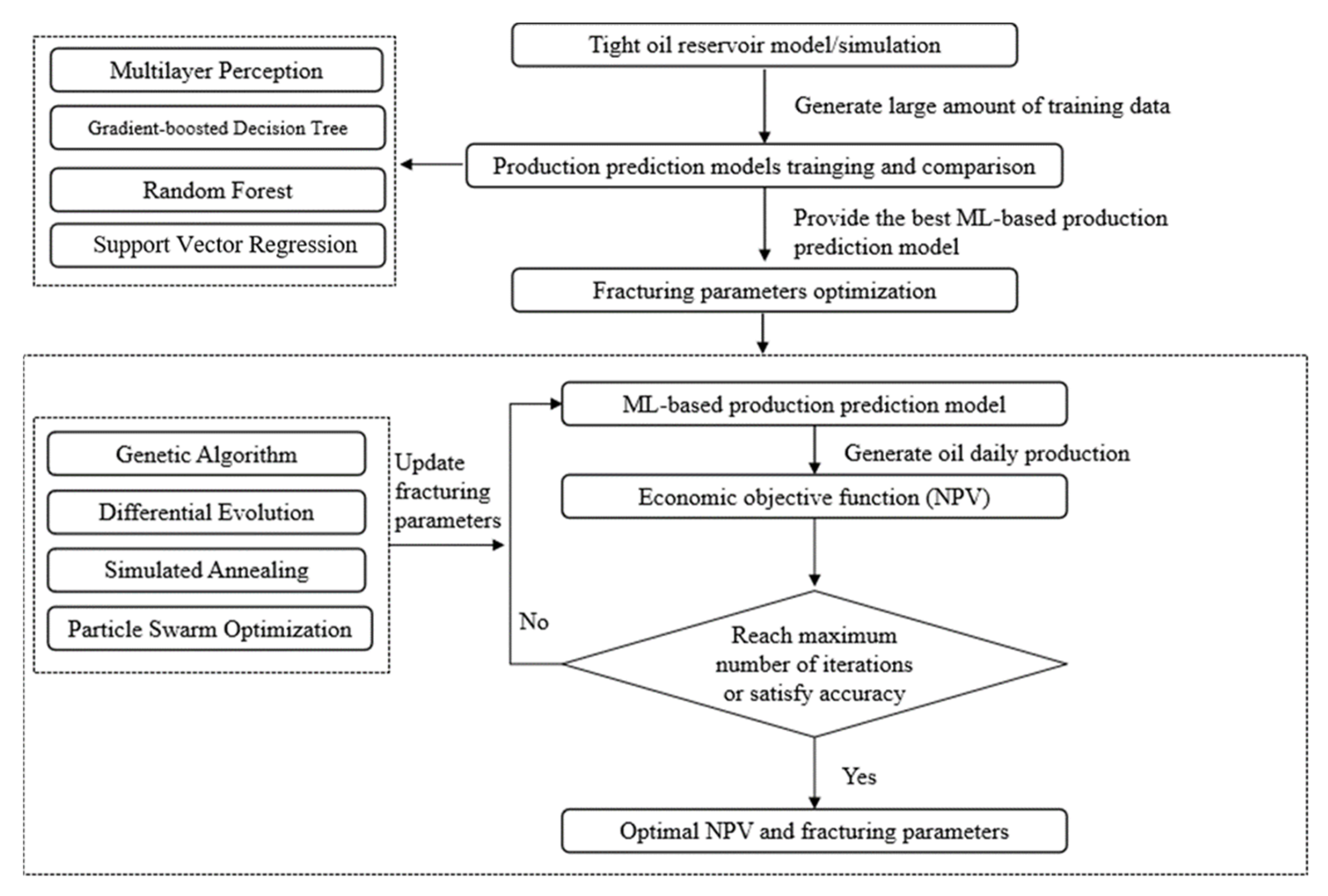
This study developed a novel hybrid model to optimize fracturing parameters by integrating the ML method and the evolutionary algorithm. This proposed methodology for modeling, predicting, and optimizing fracturing parameters was achieved in the following three major steps: first, a significant amount of production data with different geological characteristics and completion parameters was generated randomly by a numerical reservoir model. These data sets were then used to train and obtain single-well production-prediction models using various ML algorithms, after which the single-well production-prediction model with the highest prediction accuracy was selected. Finally, evolutionary algorithms were applied to the production-prediction model to optimize the fracturing parameters with the economic evaluation function, such as net present value (NPV), as the objective. As a result, the optimal economic index and corresponding optimal combination of fracturing parameters were identified. These three main steps are presented in Figure 1. The workflow can be applied to a large data set and other unconventional resources with available data as well.
2.1. Production-Prediction Model
According to the literature review on the previous oil and gas production-prediction modeling techniques, multilayer perception has been found to perform well and thus was chosen for this study. Multilayer perception is a proper machine learning (ML) technique to establish complex relationships between NPV and factors that influence it, since these relationships cannot be easily determined in a precise way. The results from previous studies indicate that the gradient-boosted decision tree (GBDT) and random forest (RF) is highly capable of solving non-linear classification problems. Another model that exhibits good performance for forecasting oil and gas production is support vector regression (SVR), which was presented and compared with other techniques in this study. The structure and components of these four widely used ML methods were briefly introduced and developed in the following section.
2.1.1. Multilayer Perception
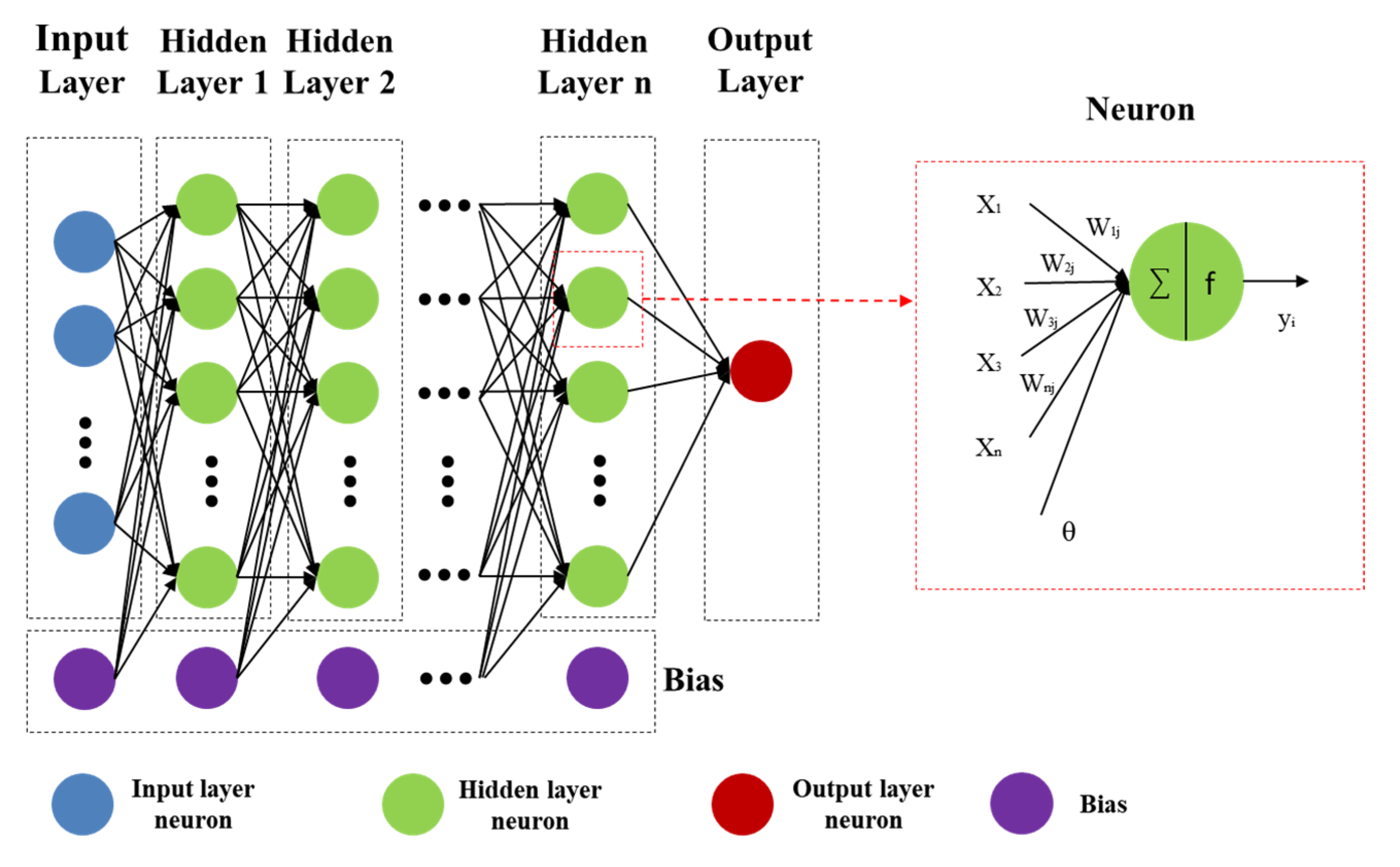
Also called ANN, multilayer perception (MLP) simulates the information-processing activity of neurons in the human brain. It is an abstract mathematical model characterized by distributed parallel information processing, and an adaptive dynamic system with a high number of extensively connected simple neurons [13]. In many ways, it matches the human approach to information processing—processing occurs as neuron interactions, knowledge, and information are stored in neuron weights, and learning and recognition depend on the dynamically evolving coefficients of neuron connection weights.
The left side of Figure 2 shows a classical neural network structure, including input, hidden, and output layers; each small circle represents a neuron, each connecting line represents a different weight that can be obtained by training, and each neuron forms a network topology by interconnecting with other neurons [14]. The right side of Figure 2 shows a mathematical model of a single neuron. Then, the input of this neuron is given as
The output of this neuron is expressed as
where is the connection weight of the ith neuron to this neuron; is the input of the ith neuron; is the activation function; and is the threshold value of the neural node in the hidden layer.
2.1.2. Gradient-Boosted Decision Tree
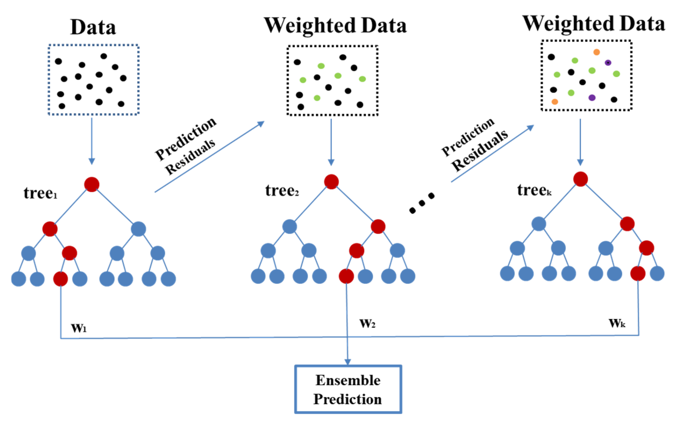
Created to ensure classification or regression, the gradient-boosted decision tree (GBDT) continuously reduces the rate of learning error resulting from the training process. It has been commonly and historically applied in the face of real production data–type imbalances [15]. GBDT is characterized by high prediction accuracy, the ability to handle consistent and discrete forms of data, the exploitation of certain robust loss functions, and extreme robustness to outliers. Each iteration of the GBDT algorithm includes a base learner called a categorical regression tree (CART), which proves suitable for high bias, low variance, and sufficient depth. An iterative process occurs in the regression problem in which each base learner is trained based on the learning error rate of the previous base learner, and then a negative gradient is fitted to the loss function using a gradient descent technique to fit the regression tree, continuously improving the decision model. The main idea of GBDT is that a new learner is trained in the gradient direction to reduce the learning error rate of the previous learner, and the new learner is generated iteratively on top of the previous learner [16,17]. Figure 3 shows a typical GBDT structure.
GBDT consists of multiple decision trees; the first m − 1 decision tree can be expressed as
The gradient of the loss function is thus obtained as
where is the sample vector and is the loss function. Then, the function of the mth decision tree is estimated as
where is the learning step.
2.1.3. Random Forest
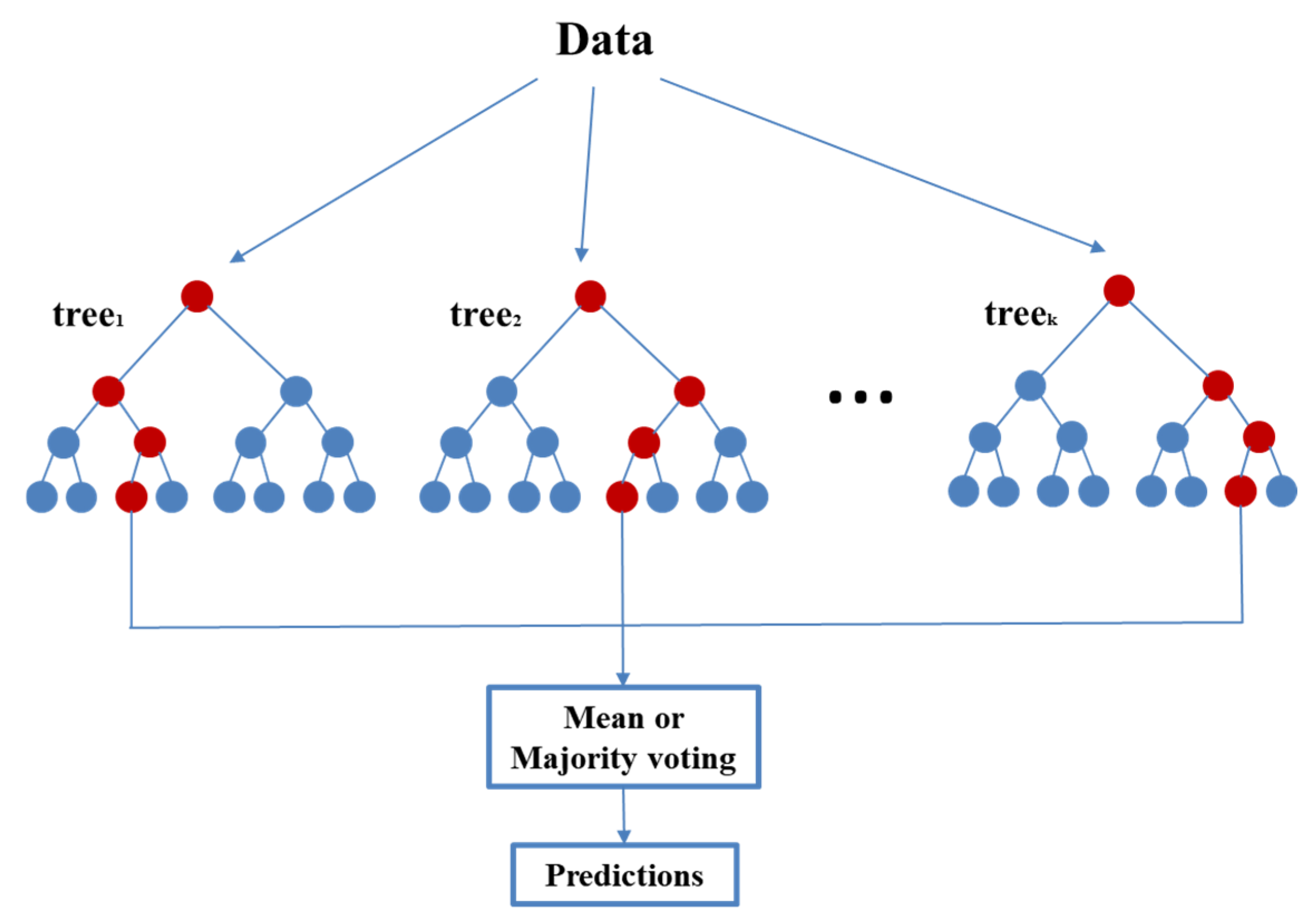
RF is a classifier that comprises multiple decision trees, with its output class identified by the plurality of the output classes of individual trees [18]. This method applies the “bagging” technique by integrating the results of multiple decision trees to find the target’s regression values and classification results. The model is a set of simple regression trees containing splits of model predictions, with each split indicating whether the observations should be used on the left or right branch of the regression tree, depending on the comparison of the threshold with a particular predictor variable. The regression tree’s final node holds the regression predictions. By randomly extracting the original training sample data with the bootstrap method and constructing a new set of subtraining samples, RF can solve the decision tree problem; the same records are kept among all the subtraining sample sets, and duplicate records are allowed among different subtraining sample sets [19,20]. Random sampling selects the best attribute. Figure 4 shows the basic principle of RF.
Using RF, if the set of regression trees is , then the final prediction is obtained by dividing the sum of the predictions of these trees for the sample by k. The mean squared random error is . When the value of k increases infinitely, it holds everywhere that
where denotes averaging about k; is the characteristic random variable; and k is the number of CART regression trees. The RF regression function is
2.1.4. Support Vector Regression
Based on the principle of structural risk minimization, support vector regression (SVR) is an ML algorithm with strong generalization ability that can overcome the problems experienced by traditional methods of overfitting and falling into local minima [21]. In a limited training sample, SVR can achieve a low error rate and can ensure that the independent test set also has a low error rate. Suppose there is a data set X containing N sample points in a K-dimensional space:
where is the ith sample of the input; is the output value; N is the total number of training samples; and K is the number of dimensions in the sample space.
The main function of the obtained optimal regression hyperplane is to make all data of a set the closest distance to that plane. The hyperplane equation is
where is the hyperplane normal and is the threshold value.
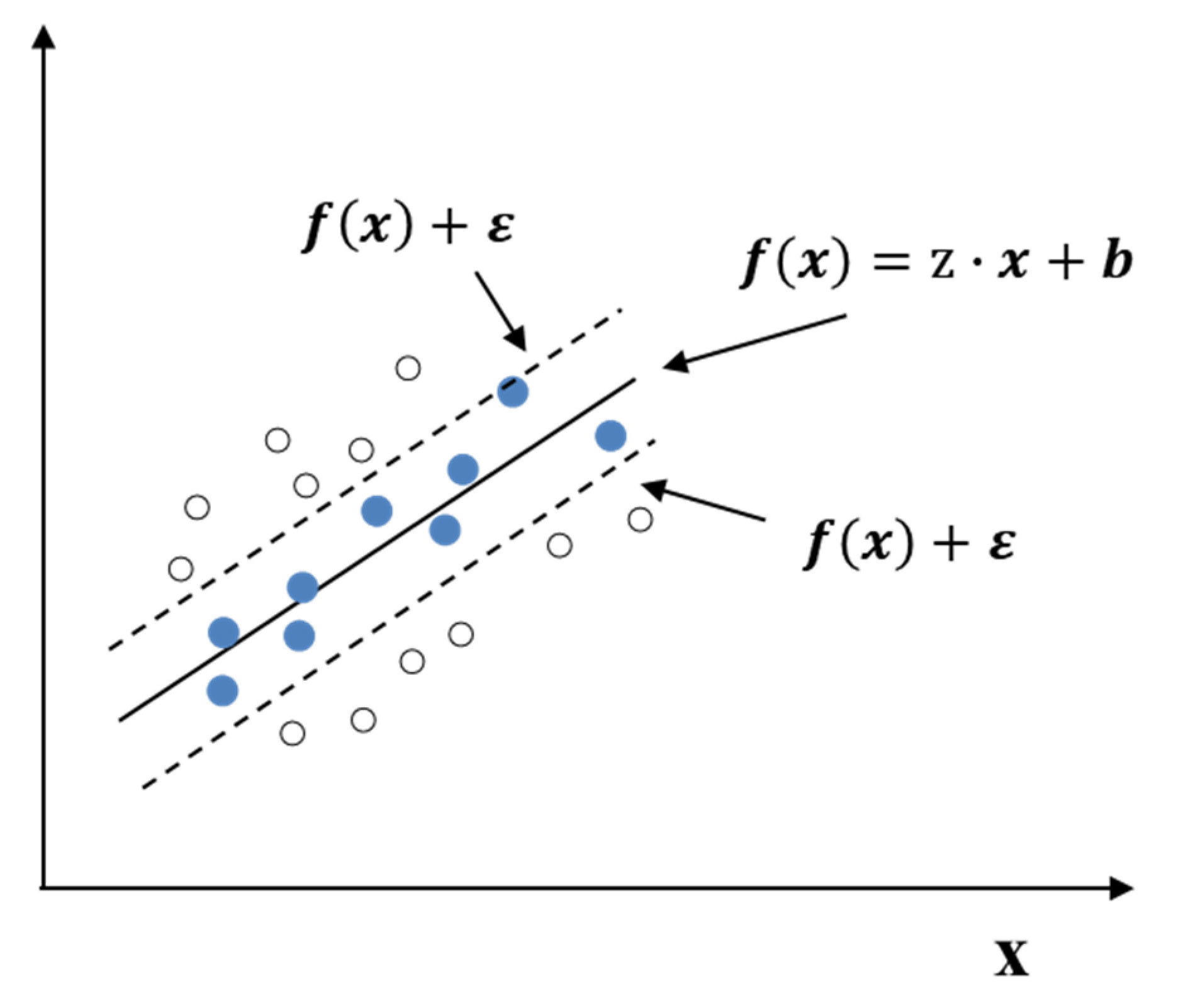
For the general regression problem, the loss of the model is zero only when and y are exactly equal, but in the SVR model, a certain degree of tolerance deviation is given so that a loss is considered when and only when the absolute value of the difference between and y is greater than the tolerance deviation . This is equivalent to constructing an isolation zone of width centered on [22,23], as shown in Figure 5.
The goal of the optimal regression hyperplane is to find the solution that minimizes the distance from all sample points to the hyperplane. Therefore, the search for the optimal regression hyperplane is changed to the optimal solution, and constraints are added as follows:
where is the hyperplane.
Because the degree of relaxation on both sides of the barrier can be different, introducing relaxation factors and , the above equation can be rewritten as
where is the regularization constant.
2.2. Fracturing Parameters Optimization
The evolutionary optimization technique searches for the optimum NPV and the fracturing parameters that affect it, using the best ML-based production-prediction model obtained in the previous section. Inspired by biological evolution, evolutionary algorithms are a “cluster of algorithms”, with many variations having different gene expressions, different crossover and mutation operators, different references to special operators, and different regeneration and selection methods. Compared to traditional optimization algorithms such as calculus-based methods and exhaustive methods, evolutionary algorithms represent mature global optimization with high robustness and wide applicability; they are self-organizing, are adaptive, are self-learning, and can effectively deal with complex problems that traditional optimization algorithms have difficulty solving, regardless of the nature of the problem [24]. The present work introduced and compared four widely used evolutionary algorithms: genetic algorithm (GA), differential evolution algorithm (DEA), simulated annealing algorithm (SAA), and particle swarm optimization (PSO).
2.2.1. Genetic Algorithm
GA simulates an artificial population’s evolution and, through the mechanisms of selection, crossover, and mutation, iteratively searches for the approximate optimal solution [25]. First, GA initializes the population, including the determination of population size, the iteration number, and the chromosome codification. The genetic algorithm identifies the encoding and decoding processes for problem solving, which generally takes real-number encoding or binary encoding, depending on the specific problem-solving design. The GA population consists of a population of individuals, one of which is characterized by a string of variables, that is, a gene, and generating the initial population occurs according to the rules. For each iteration, GA calculates the fitness of the individuals, that is, how well they match the problem. The higher the value of fitness, the higher the quality of the solution. In each iteration, the population experiences three steps: selection, crossover, and mutation. Selection means choosing the better adapted individuals to pass into the next-generation population and eliminating the less adapted individuals. Crossover is the exchange of gene sequences among pairs of individuals, which effectively improves GA’s ability to search for solutions. Mutation is the change in gene values in individual gene sequences. The mutation operation gives GA a local random search capability and enables it to maintain population diversity, preventing the algorithm from converging prematurely. The algorithm terminates when the number of iterations or the fitness of the best individual in the population reaches a certain threshold. The relative optimal solution is the individual with the best fitness in the population.
2.2.2. Differential Evolution Algorithm
Like GA, the DE optimization algorithm is based on modern intelligence theory; through group intelligence generated by mutual cooperation and competition among individuals in the group, it guides the optimization search [26]. Its main working mechanism is similar to GA, but the sequence of its main steps is mutation, crossover, and selection. The basic idea of the algorithm is as follows: starting from a randomly generated initial population, a new individual is generated by summing the vector difference of any two individuals in the population with a third individual and then comparing the new individual with the corresponding individual in the contemporary population. If the fitness of the new individual is better than the fitness of the current individual, the current is supplanted by the new in the next generation; otherwise, the current is retained. The good individuals are kept, and the bad individuals are removed, through continuous evolution, and the search is guided to approach the optimal solution. Unlike GA, the DE algorithm’s variance vector is generated from the parent differential vector and is crossed with the parent individual vector to create a new individual vector, which is selected directly with its parent individual.
2.2.3. Simulated Annealing Algorithm
The SA algorithm hails from the principle of solid annealing, in which a solid is heated to a sufficiently high temperature and then is allowed to cool down slowly [27]. When the temperature rises and internal energy increases, the particles inside the solid become disordered; when cooled slowly, the particles reorder, reach the equilibrium state at each temperature, and finally reach the ground state at room temperature when the internal energy is reduced to a minimum. A stochastic optimization algorithm, the SA algorithm is based on the Monte-Carlo iterative solution strategy; its starting point is the similarity between the annealing process of solids in physics and general combinatorial optimization problems. The SA algorithm starts at a certain high initial temperature, applies a decreasing temperature parameter, and combines the probabilistic jump property to randomly search for the global optimal solution of the objective function in the solution space, that is, the local optimal solution can probabilistically jump out and eventually converge to the global optimal.
2.2.4. Particle Swarm Optimization Algorithm
The particle swarm optimization (PSO) algorithm is an intelligent optimization algorithm based on group collaboration and global search, inspired by the migration and flocking behavior of the foraging process of birds [28]. In the PSO algorithm, each particle is first initialized randomly to get its initial position and velocity. In the process of searching the global optimal position, each particle carries the following two pieces of information: current position and current velocity. Then, the PSO algorithm changes the adaptation value of the particles through the objective function. Both the optimal position found by the particle itself (called individual extreme value, Pbest) and the optimal position found by the whole population (called global extreme value, Gbest) are obtained through real-time comparison [29,30]. Assuming that the initial population consists of e particles, and the position and velocity of the ith particle are denoted as and , the following update equations for the velocity and position of the particles are obtained:
where k is the current number of iterations; ω is the inertia weight; and are the learning factors; affects the weight of the local optimum; affects the weight of the global optimum; and are random numbers of [0, 1]; and are the velocity and position of the ith particle’s flight velocity vector; and and are the current individual extremes and global extremes of the particle, respectively.
The particle fitness function is given as:
where p is the number of training samples; q is the number of test samples; is the true value of the training samples; is the predicted value of the training samples; is the true value of the test samples; and is the predicted value of the test samples.
3. Data Preparation and Generation
Building a data-driven production-prediction model requires a significant number of static and dynamic data (logs, fracturing, production, etc.) as input, and then ML methods establish correlations between static and dynamic data. Ideally, the data set used to construct the data-driven model is taken from the real domain. However, synthetic data obtained from numerical or analytical simulations can be used if high-quality real data are insufficient or unavailable [31]. In this section, we describe how we prepared the geological and completion parameters for the study area and generated production profiles as inputs for the data-driven production-prediction model.
3.1. Study Area
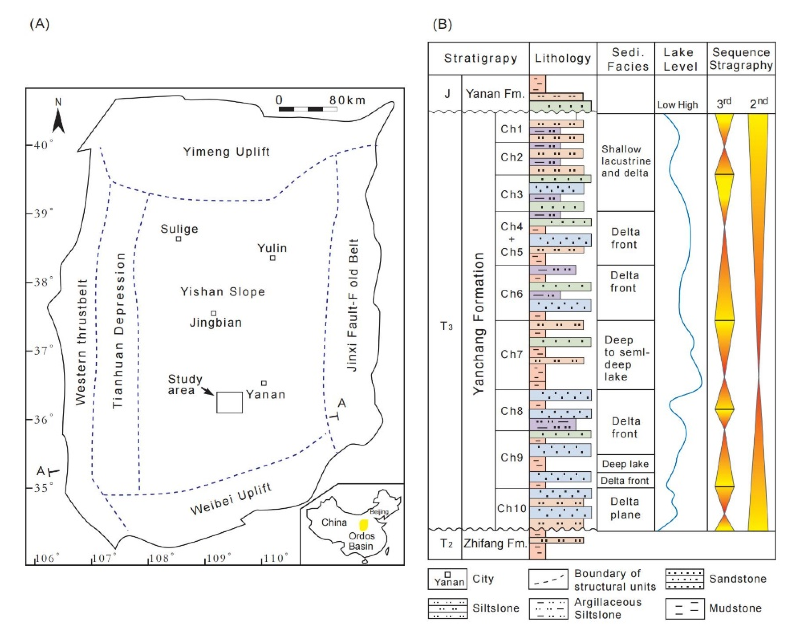
Located at the tectonic intersection of the east–west region of China, the Ordos Basin is part of the Paleozoic Greater North China Basin (Figure 6A). The movement of the Late Triassic Indochinese West Island led to the collision of the northern margin of the Yangtze Plate with the North China Plate, and the Ordos formed a large-scale inland lake basin. The basin is divided into six secondary tectonic units—the western margin thrust belt, the Tianhuan depression, the Yishaan slope, the Jinxi flexural fold, the upper slope of the metabolism, and the upper slope of Weibei [32]. The Liuluoyu area of the Xiasiwan oil field is located in the southern part of the Ordos Basin’s Yishaan slope (Figure 6A). The regional structure is a gentle monocline with a stratigraphic dip less than 1o; a slope drop of 6 to 9 m/km; a simple internal structure; and a low-amplitude, nose-like uplift formed locally by differential compaction. The Liuluoyu area is an important oil-bearing block in northern Shaanxi. From top to bottom, it is divided into rock groups Chang 1 to Chang 10 (Figure 6B). The Chang 8 reservoir in the study area is a typical rocky reservoir not controlled by the tectonic high point, with oil–water mixed storage, no obvious edge or bottom water, and a lithology comprising mainly sandstone of sharp extinction or dense layer blocking. The reservoir drive type is elastic-dissolved gas, the oil-bearing height in this area is 45 m, the depth of burial at the high point of the reservoir is 1460 m, the central elevation is −220 m, and the average depth of burial of the oil layer is about 1668 m. The reservoir properties significantly vary across the study area, with permeability ranging from 0.0001 to 1 mD and porosity ranging between 5 and 15%.
3.2. Data Generation
Geological, petrophysical, and reservoir properties are important factors affecting tight oil productivity. To select geological parameters for the ML model, we investigated the key impacts on tight oil production: drainage area, porosity, permeability, reservoir pressure, and bubblepoint pressure [34,35]. In addition, various studies have found fracture design to play a key role in the stud area’s well productivity. Fracturing parameters such as fracture permeability, fracture spacing, and fracture length are essential to economic success.
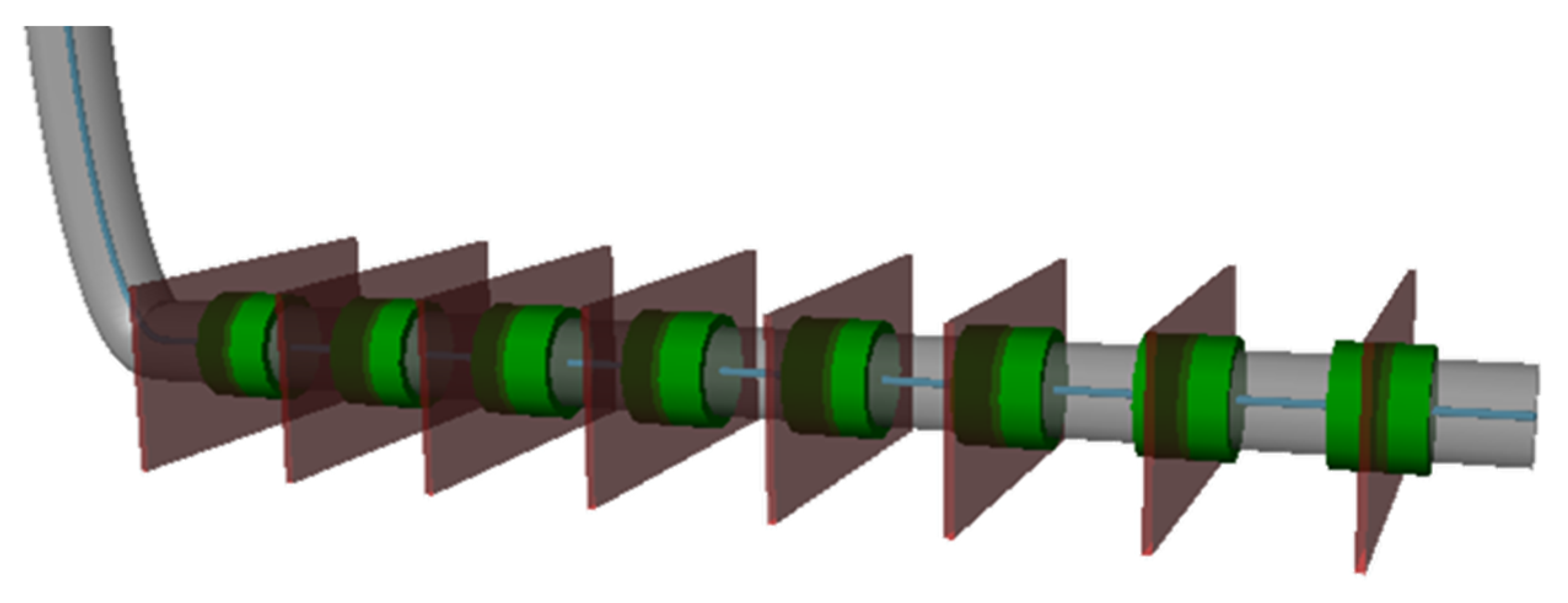
The multistage hydraulic fracture model of a tight oil well established in this study was a three-phase, 3D, rectangular model. In recent studies, four major methods have been commonly used to model fractures, including the analytical model [36], local grid refinement (LGR) [37], continuum approaches [38], and the embedded discrete fracture model (EDFM) [39]. Because of its fast computing speed and high flexibility, the ECLIPSE commercial simulator with LGR was applied in this study to model complex hydraulic fracture geometries. The synthetic reservoir model comprises one horizontal well and eight transverse hydraulic fractures perpendicular to the wellbore. The reservoir model was discretized into 50 × 21 × 7 grid blocks. The horizontal well is designed in the center of the reservoir model and is assumed to produce under a constant bottomhole pressure (BHP). In LGR, the grid blocks around the hydraulic fracture were logarithmically refined to address the large pressure drop. The production period was set to 10 years, which is considered as a realistic tight oil production scenario. The numerical reservoir model is shown in Figure 7.
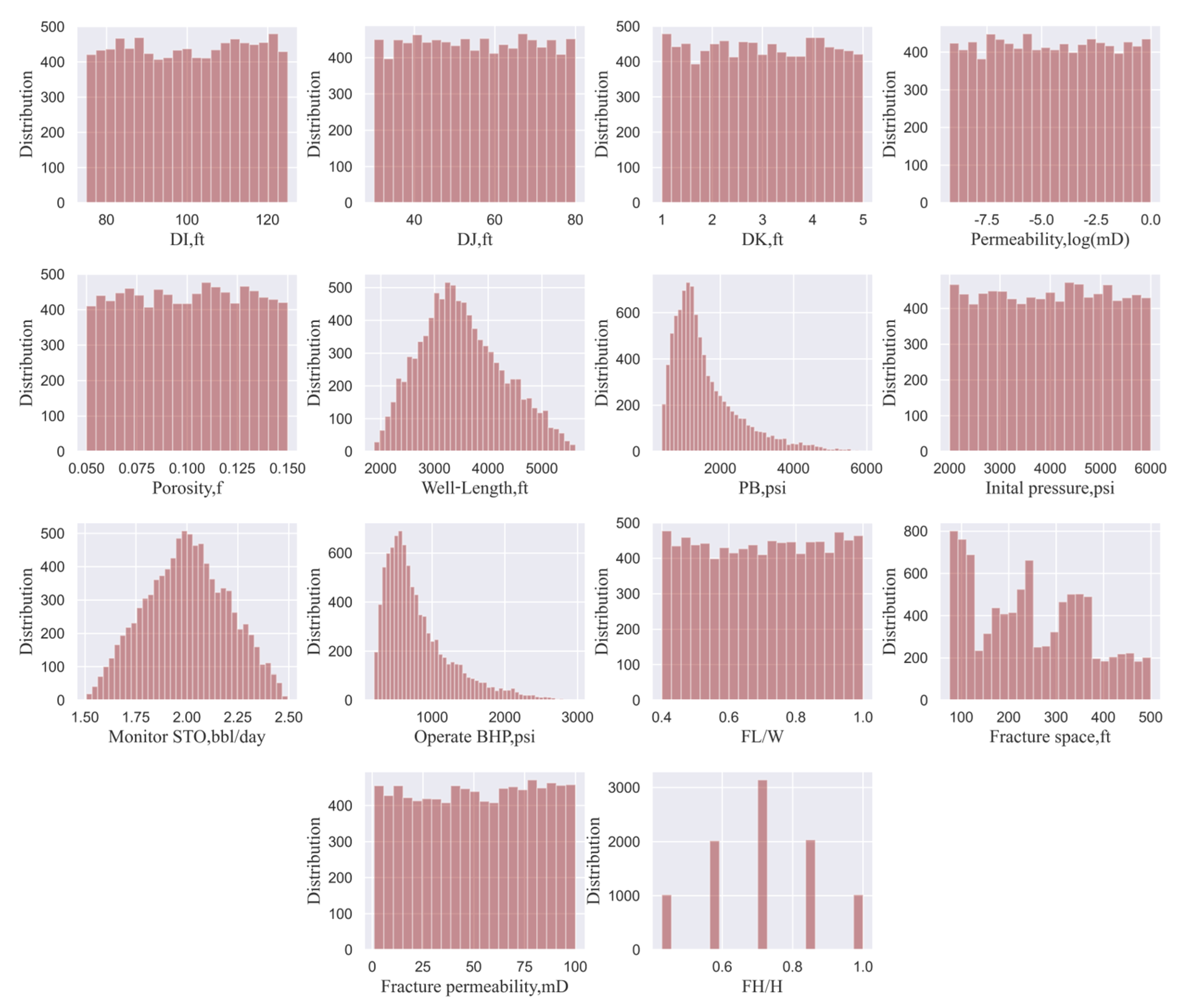
In total, 14 reservoir and fracturing parameters were selected and considered in this study, including the X, Y, and Z directional grid sizes (DI, DJ, and DK); horizontal well length; matrix permeability; matrix porosity; initial pressure; bubblepoint pressure; monitored oil rate; operating BHP; average fracture length/reservoir width; fracture spacing; fracture effective permeability; and average fracture height/reservoir height (Table 1). Of these 14 parameters, the first three parameters define the size of the model; they were used as a proxy for the drainage area in this study. Thus, these three parameters directly affect the initial oil in place, as well as tight oil production. To ensure horizontal well length being confined by reservoir length, for instance, the well length was set at the reservoir length times a random number between 0.6 and 0.8. Matrix permeability and matrix porosity represent the rock properties of tight oil reservoirs. The initial pressure determines the initial condition of the reservoir, while bubblepoint pressure is one of the most important characteristics that defines the fluid properties. Four characteristics—average fracture length/reservoir width, fracture spacing, fracture effective permeability, and average fracture height/reservoir height—define the fracturing parameters of the horizontal well. Instead of (effective) fracture half-length, fracture length/reservoir width was used because it helps to visualize the degree of fracture propagating in the drainage area. The values ranged from 0 to 1, indicating fracture length being confined by reservoir width. The same applied to the ratio of fracture height/reservoir height.
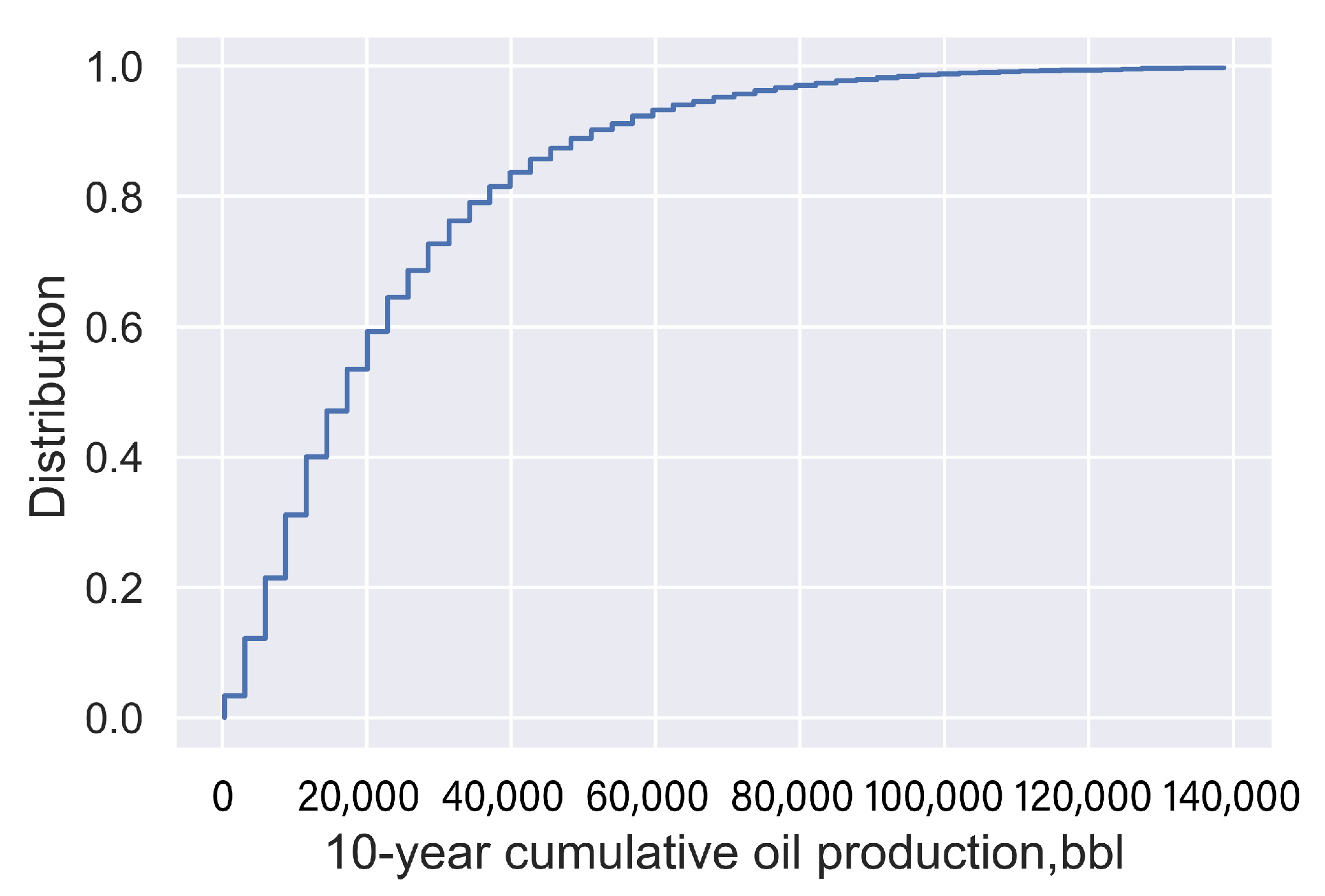
We collected geological and completion data from Xiasiwan oil field’s database and determined the range and distribution of the 14 selected parameters (listed in Table 1) based on the 10,000 sets of geological and completion parameters generated by the Latin hypercube sampling (LHS) technique. The probability distribution of each parameter is shown in Figure 8. The output of the production model was monthly oil production for 10 years, numerically simulated by each combination of geological and completion data sets. Figure 9 shows the cumulative probability distribution of 10,000 cumulative oil productions for the 10-year production period.
4. Results Analysis
4.1. Comparison of the Data-Driven Production-Prediction Models
The geological characteristics, hydraulic fracturing parameters, and corresponding tight oil production from the 10,000 wells generated and presented in Section 3.2 were used to establish the data-driven production-prediction model. The fixed division of the training and test set would result in severe overfitting issues. To avoid possible overfitting, we applied the k-fold cross-validation (k = 8) to characterize the prediction performance and generalization ability of the ML model. K-fold method can obtain a comprehensive evaluation metric of the model by changing the training and test set.
To develop the production-prediction model, four ML algorithms—SVR, GBDT, RF, and MLP—served as mapping functions to establish the relationship between static and corresponding dynamic data. Table 2 shows the final hyperparameters of the four models used to achieve optimal results for this study, which were obtained by trial and error.
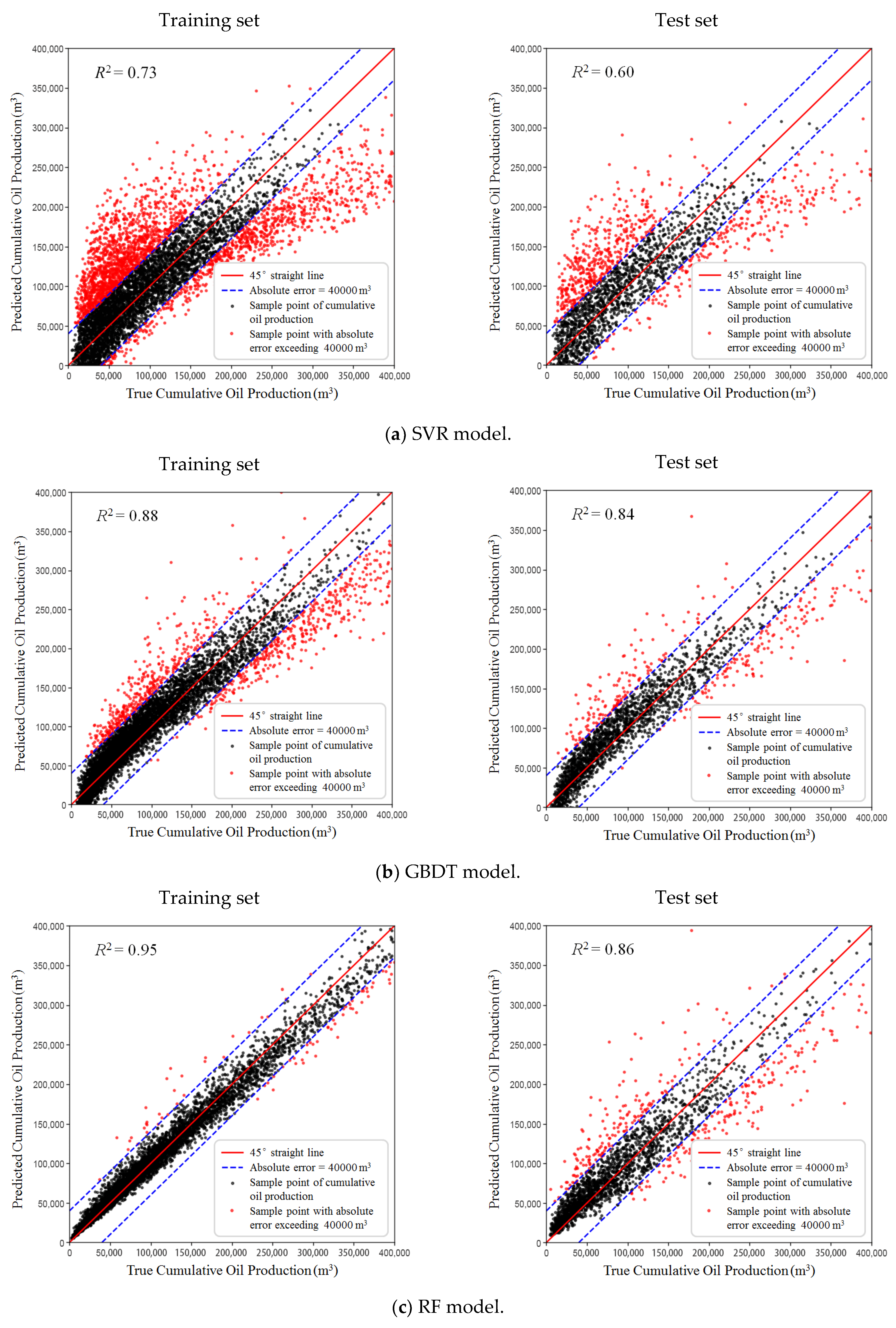
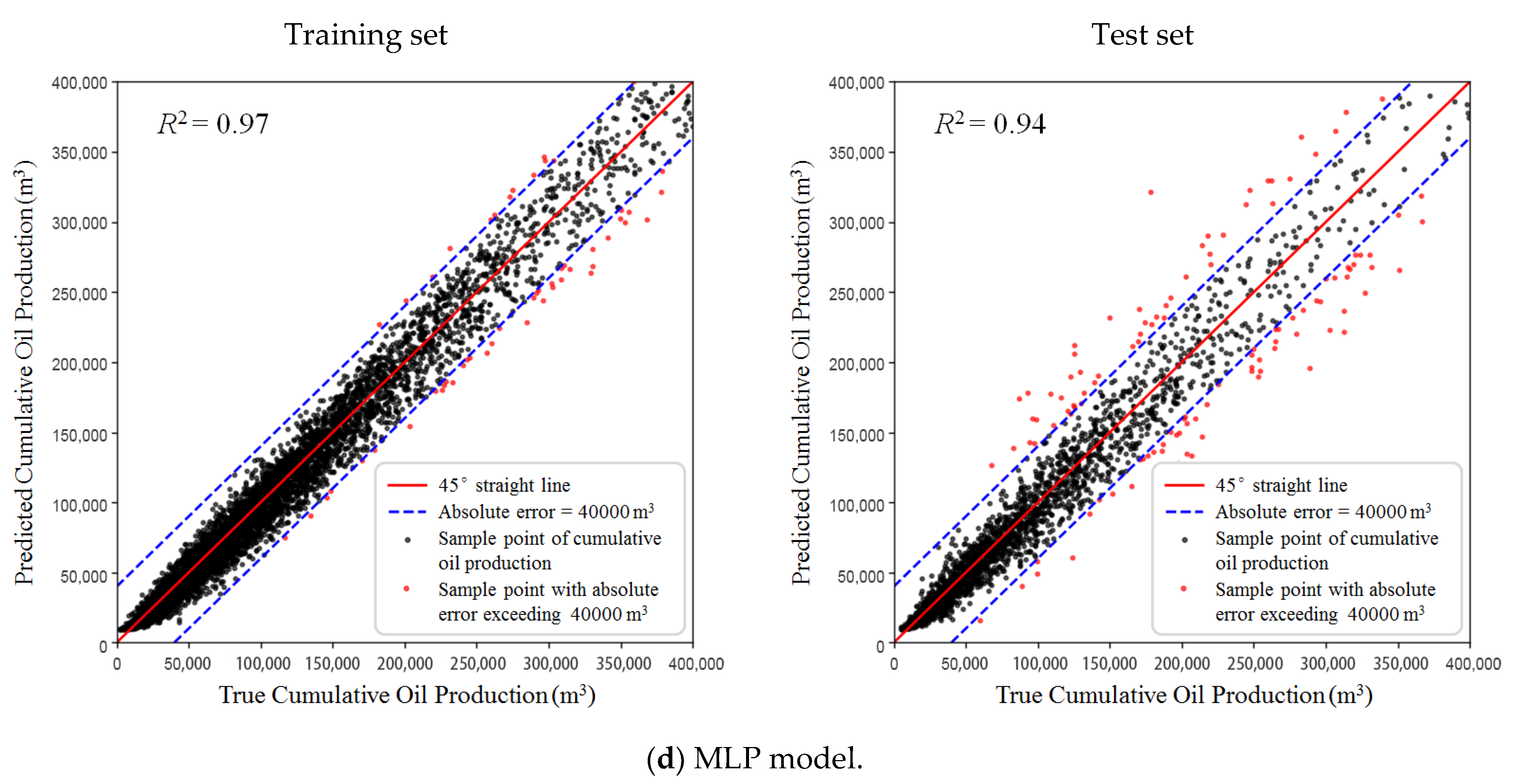
Figure 10 shows scatterplots of true-versus-predicted cumulative production of all the training and testing set for the four prediction models. The solid red 45° line in each subplot indicates that the predictions are equal to the actual data. The area enclosed by the two blue dash lines contains all the samples whose absolute errors of cumulative oil production are less than 40,000 m3. The smaller the difference between the predicted and actual values, the closer the data points approaching the 45° line. The values obtained by RF and MLP models (Figure 10d,e, both the training set and testing set) are mainly distributed along the 45° line, which indicates both models achieved high prediction accuracy.
To further quantify the prediction precision of the four data-driven production-prediction models, we selected the correlation index (R2) as a metric [40], which is shown in Equation (15). The R2 value is between 0 and 1. A high value indicates a good match, while a low value means a bad match.
The mean R2 obtained with k-fold cross validation of the four prediction models is given in Table 3, where the RF and MLP models show higher R2 values. RF, though, is seen to have an overfitting phenomenon, causing its R2 value in the test set to be 10% lower than that in the training set, meaning that the RF algorithm has focused on the training set so much that it has missed the point entirely. In this way, the RF model can produce good predictions for data points in the training set but performs poorly on new samples. Thus, MLP was determined to be the optimal algorithm to establish the production-prediction model for this study.
4.2. Effect of Sample Size on the Predictive Performance of the MLP-Based Model
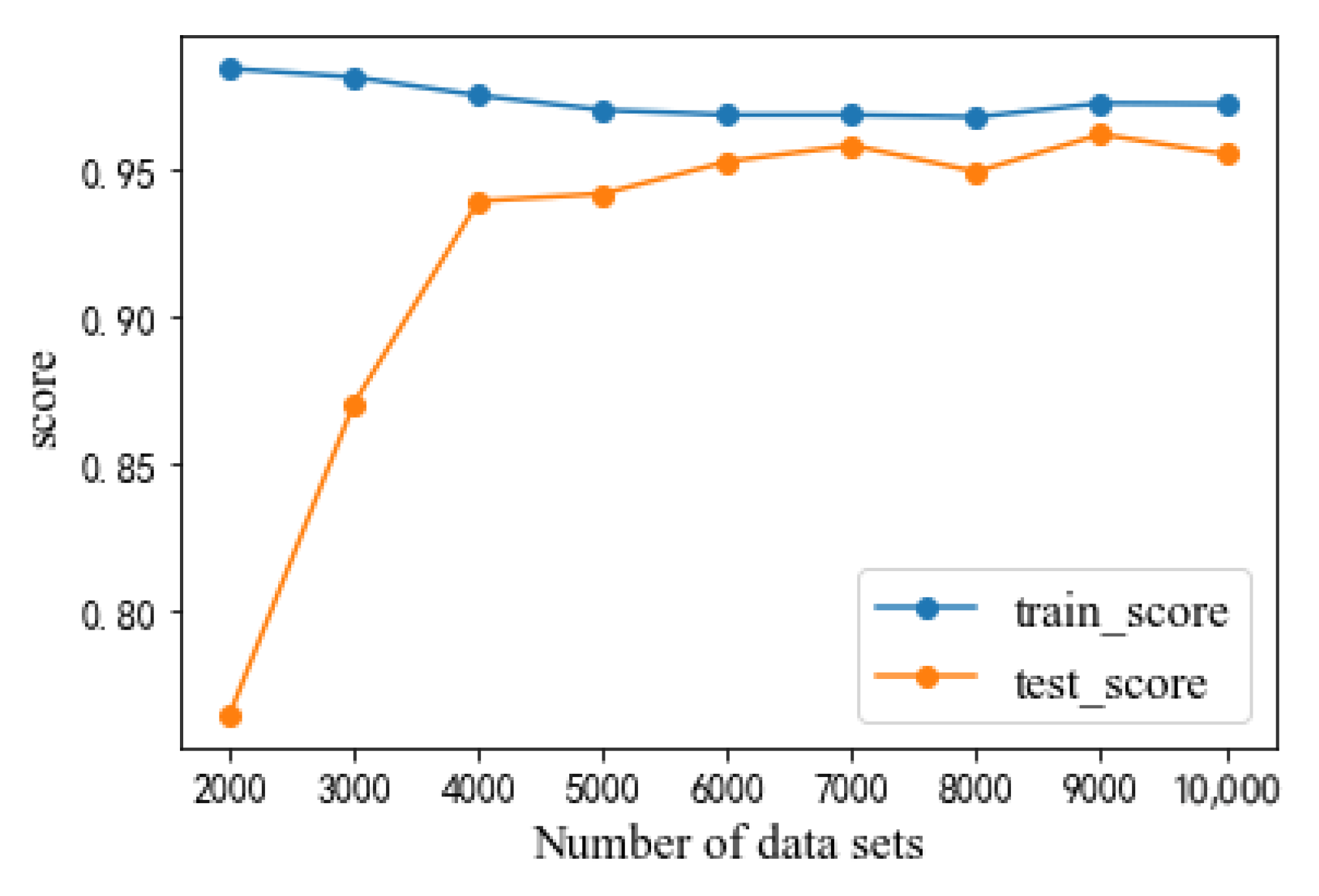
It is reasonable to ask what the required sample size is to build an MLP-based production-prediction model. To figure out how many data sets are representative enough for the tight oil production-prediction model, we conducted a systematic analysis with nine different total sample sizes, varying from 2000 to 10,000. Figure 11 shows the R2 scores for both the training and test sets of each sample size. Generally, it can be observed that test set accuracy increases with sample size and training set accuracy decreases with sample size. The test set increase is more obvious when the total sample size is under 4000, with the increase rate starting to slow down after that. The MLP model is seen to be overfit when the total sample size is small (under 4000), and as the total sample size increases, the overfitting gradually improves. When the total sample size approaches 6000, the accuracies of the training and test sets nearly stabilize, with only a negligible amount of improvement. Thus, the trained MLP-based data-driven model with a total sample size of 6000 was further used as the final single-well production-prediction model to optimize the fracturing parameters in the next step.
4.3. Effect of Fracturing Parameters on Cumulative Oil Production
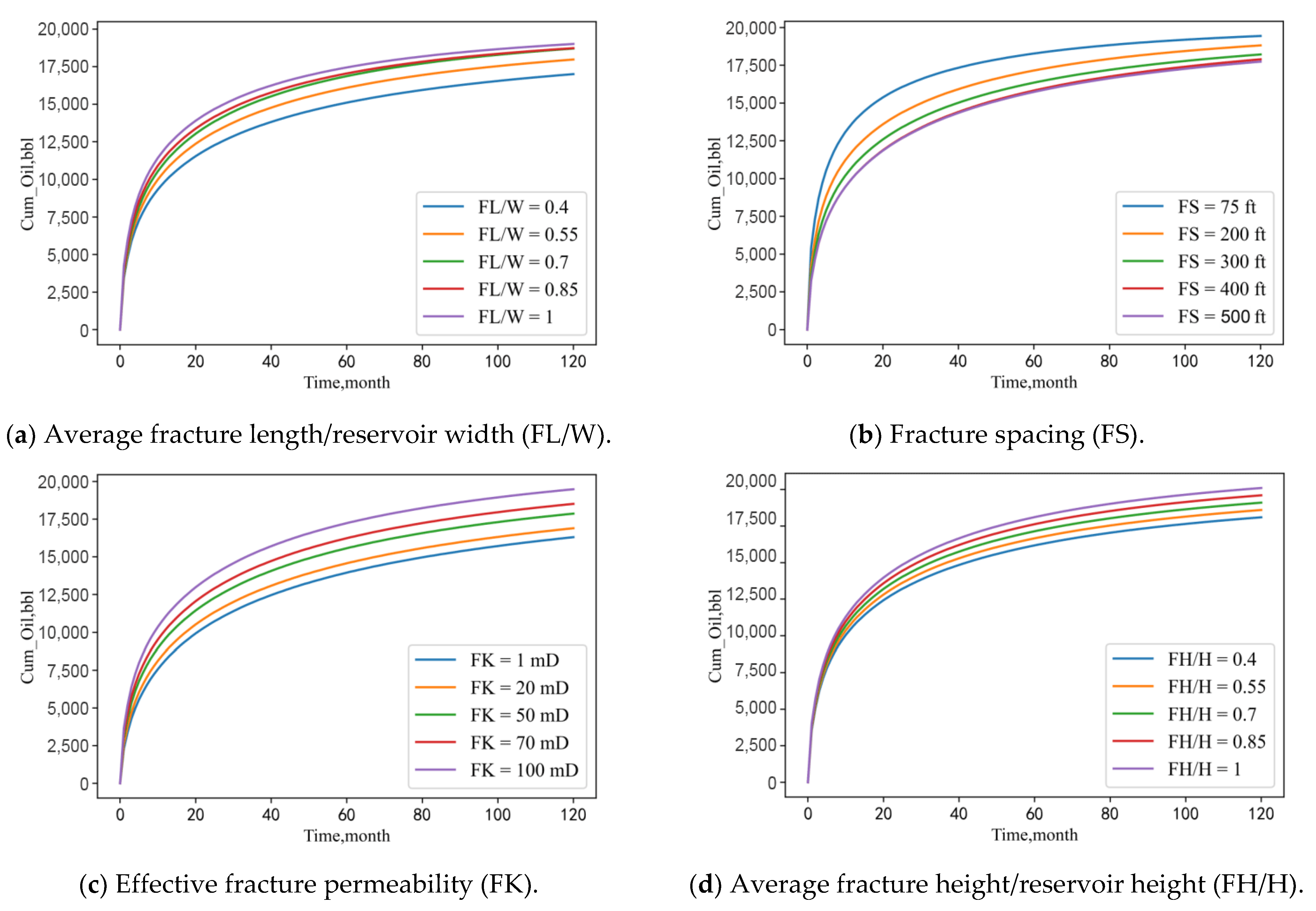
The key attributes in fracturing parameter optimization were found to be fracture length/reservoir width, fracture spacing, effective fracture permeability, and fracture height/reservoir height. A sensitivity analysis was performed to investigate the effect of these four fracturing parameters on cumulative oil production. The base case was established, with Table 4 showing its 14 parameters. The MLP-based production model obtained with 6000 sets of data was used to calculate oil production.
Figure 12 shows the sensitivity of cumulative oil production to fracturing parameters for the parameter settings of Case 1. Figure 12a shows the effect of fracture length/reservoir width on cumulative oil production. The longer the fracture length/reservoir width, the higher the cumulative oil production. Figure 12b indicates that the tighter the fracture spacing, the higher the cumulative oil production. Figure 12c means that high effective fracture permeability can greatly increase oil production. Figure 12d shows that the cumulative oil production increases with fracture height/reservoir height, but its change does not affect cumulative oil production. It can be concluded from the sensitivity analysis that cumulative oil production is more sensitive to fracture length/reservoir width, fracture spacing, and fracture effective permeability and less sensitive to fracture height/reservoir height.
4.4. Techno-Eco-Analysis Scheme of Tight Oil Projects
We first define the economic objective function that considers fracturing treatment cost and oil production benefit and integrate the evolutionary algorithms with the MLP-based production-prediction model to obtain the optimal combination of fracturing parameters that corresponds to the optimal economic feasibility.
4.4.1. Definition of Economic Objective Function
The most commonly used index to evaluate the feasibility of a project is NPV. Different mathematical expressions for NPV exist under different assumptions, but they usually consist of two components: discounted cash flow and capital expenditure (CAPEX).
Periodic net cash flow (NCF) is defined as
where is the oil production rate at time step t; and are oil price and operation cost per unit; and R represents tax rate.
The CAPEX of a project includes the investment of drilling and fracturing and fixed cost:
where is the drilling cost of the horizontal well; is the fixed cost; and is the fracturing cost, calculated as:
where ,, and represent fracturing costs associated with fracturing fluid, proppant, and base treatment cost, respectively, which can be estimated by the following equations provided by the operator:
where N is the fracturing stage number, FL is the fracture length, FW is the fracture width, and FH is the fracture height. Thus, the objective was to maximize the NPV function expressed as follows:
where n is the total number of time steps considered in the cash flow calculation. Table 5 gives the value of main economic parameters.
4.4.2. Effect of Fracturing Parameters on Net Present Value
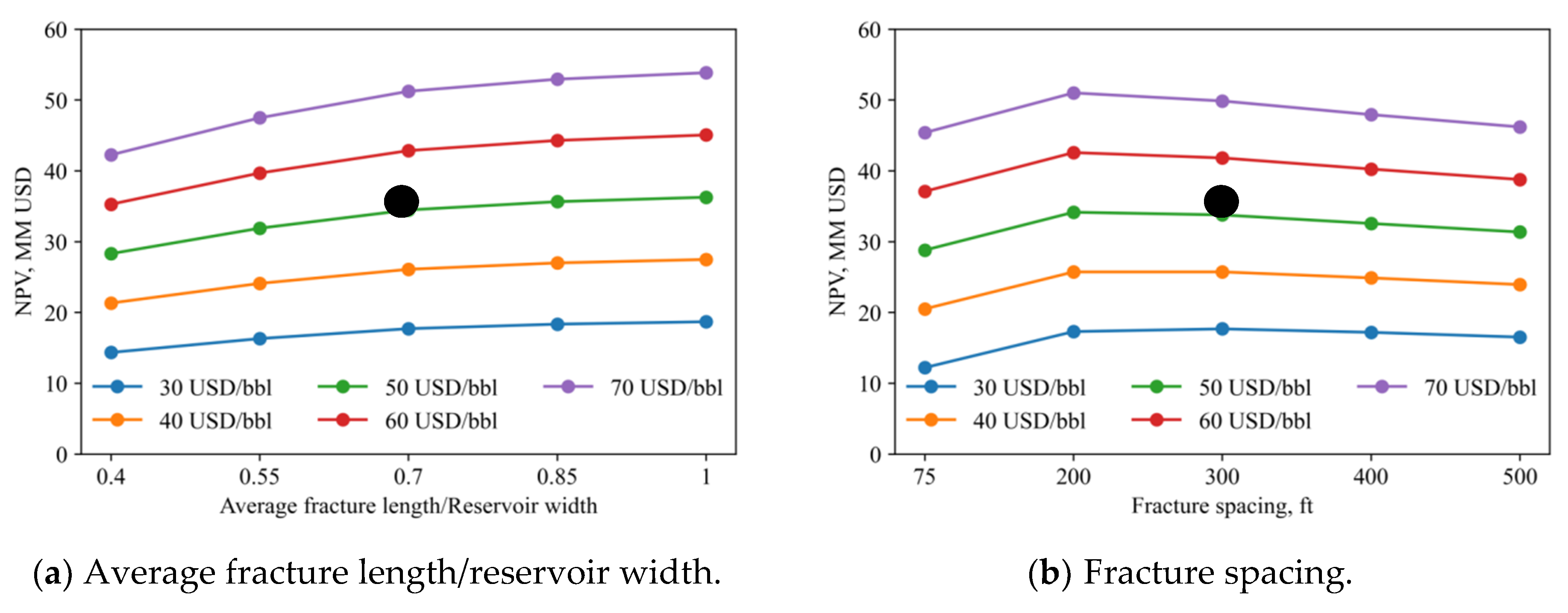
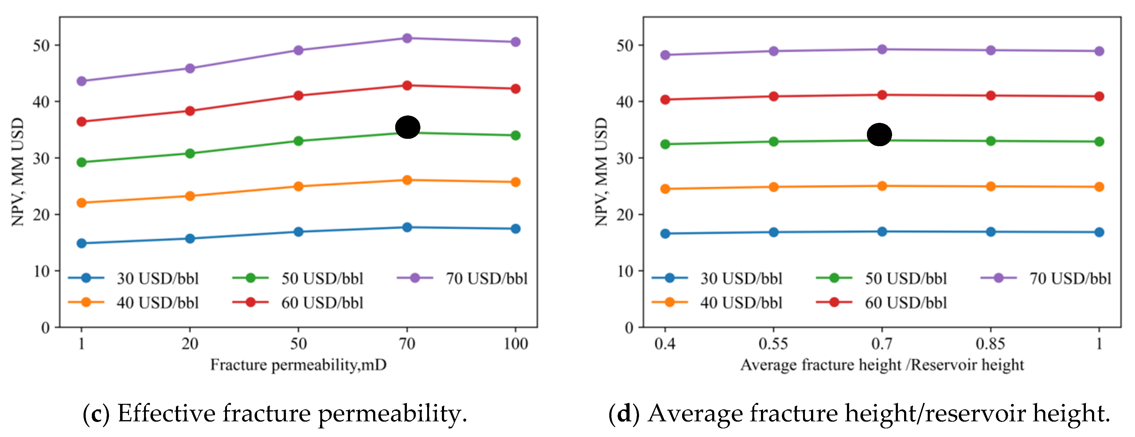
To investigate the impact of fracturing parameters on economic evaluation, the sensitivity of NPV to fracturing parameters was analyzed for four different oil prices. The base case established for NPV sensitivity analysis was the same as that for cumulative oil production.
Figure 13a shows the effect of fracture length/reservoir width on NPV at different oil prices. The black dot in each subplot represents the NPV values obtained from the base case. It can be seen that NPV increases as fracture length/reservoir width increases. Figure 13b shows the optimal fracturing spacing between 200 and 300 ft. Figure 13c shows fracture permeabilities having a positive effect on NPV. Figure 13d indicates that NPV is not sensitive to fracture height/reservoir height.
4.4.3. Integration of Evolutionary Algorithms and Multilayer Perception
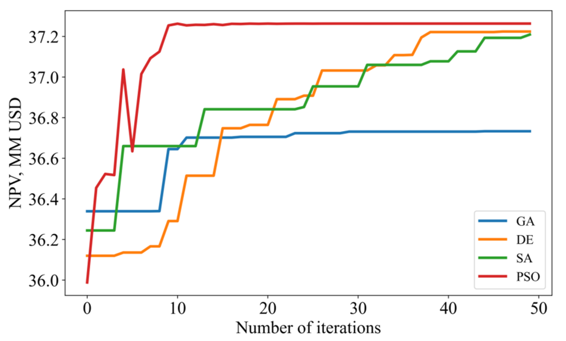
In this study, four evolutionary algorithms—GA, DE algorithm, SA algorithm, and PSO—were integrated with the MLP-based production model to optimize the fracturing parameters of the base model (Table 4); the ideal fracturing parameter optimization algorithm was selected by comparing their iteration speeds and optimal NPVs. Table 6 summarizes the final hyperparameters of the four optimization algorithms.
Figure 14 shows the trend of NPVs with the number of iterations for the four algorithms. It is obvious that the NPV generally increases with the number of iterations, and then it tends to be stabilized. The final combination of fracturing parameters obtained by the four optimization algorithms and the performance indexes is shown in Table 7. Among the four methods, MLP-PSO tends to stabilize at Iteration 8 and achieves the highest NPV value of USD 37.26 million. Overall, the MLP-PSO method outperformed the other three algorithms at convergent speed, with an optimal value achieved.
5. Discussion and Future Work
Conventional workflows for well completion and production optimization in tight oil reservoirs require extensive earth modeling, hydraulic fracture simulation, and production simulation. This methodology is data-intensive and time-consuming and often is not rigorously accomplished because of a lack of skillset and time. In addition, a complete understanding of the impact of each parameter and the correlations among them is very difficult to obtain. Considering the potential value of this study on fracture design optimization, overcoming the above-mentioned limitations becomes critical. To do so, conducting single-well reservoir simulations, analyzing the results using ML algorithms, and optimizing fracturing parameters with evolutionary algorithms can help to develop a powerful solution that creates “proxy” models for fast and effective fracture optimization.
Given the flexibility of ML, the production-prediction model used in this study still has room for improvement. For instance, the structure of the MLP model can continue to be optimized by setting a more appropriate number of hidden layers and of neurons, a more appropriate learning rate, etc. The debugging of these hyperparameters can also provide the model with better prediction accuracy, and even optimization algorithms such as PSO and GA can be added in this step to optimize the MLP model. In addition, ML methods are developing rapidly and can use convolutional neural networks (CNNs) to better mine the features of parameters; LSTM networks to better preserve the temporal features of parameters; or even hybrid networks, such as CNN-LSTM and CNN-GRU. It is believed that these models not only will provide more flexibility and alternatives, but they will also make the problem more challenging because with too many options available, debugging becomes more difficult. The objective function for optimizing the economic evaluation in this study was NPV, but the NPV calculation ignores taxation, which was not considered comprehensively enough and can be improved in subsequent studies. Moreover, the economic evaluation of this study only considered the optimization of a single objective function, i.e., NPV, and subsequent studies can consider multiobjective optimization, such as the cumulative water-to-oil ratio and fracturing fluid efficiency using the Pareto method.
6. Conclusions
In this study, a robust workflow is proposed for optimizing fracturing parameters by coupling ML methods and optimization algorithms. We optimized fracturing parameters, including fracture half-length, fracture permeability, fracture spacing, and fracture height. The workflow provides a new alternative to solve the dimension-varying problem by considering various fracturing parameters. Specific observations and conclusions follow:
- 1.
- Compared with traditional statistical methods and numerical simulation methods, ML can make the comprehensive use of various factors such as geological, completion, and production parameters and can effectively deal with field data and nonlinear problems without the limitations of geological models, thus quickly establishing reliable production prediction and greatly improving model prediction accuracy and efficiency.
- 2.
- Among the four ML models, the MLP model shows the best production-prediction performance.
- 3.
- The sensitivity analysis of fracturing parameters was conducted on cumulative oil production. It was found that cumulative oil production is more sensitive to fracture length/reservoir width, fracture permeability, and fracture spacing. It is less sensitive to fracture height/reservoir height. Cumulative oil production is positively correlated with fracture length/reservoir width, fracture permeability, and fracture height/reservoir height and is negatively correlated with fracture spacing.
- 4.
- From the sensitivity analysis of the NPV fracturing parameters, a range of optimal values can be roughly determined for the four fracturing parameters.
- 5.
- Comparing the four fracturing parameter optimization models, the MLP-PSO model shows better performance than the other three models, both in convergence speed and optimal value.
Author Contributions
Conceptualization, Z.D.; Data curation, L.W. (Lei Wu) and L.W. (Linjun Wang); Resources, Z.W. and Z.L.; Writing—original draft, Z.D.; Writing—review and editing, W.L. All authors have read and agreed to the published version of the manuscript.
Funding
We would like to thank the Project “Shale Gas Production Prediction Base on Machine Learning Algorithms” funded by RIPED-PetroChina, the Project of National Natural Science Foundation of China (grant nos. 51974253 and 51934005), the Natural Science Basic Research Program of Shaanxi (Grant No. 2017JM5109), and the Shaanxi Province Key R&D Program “Small Molecule Recyclable Self-Cleaning Fracturing Fluid R&D and Industrialization Promotion (Project No.: 2022ZDLSF07-04)”, for their financial support and valuable data.
Institutional Review Board Statement
Not applicable.
Informed Consent Statement
Informed consent was obtained from all subjects involved in the study.
Data Availability Statement
Not applicable.
Conflicts of Interest
The authors declare no conflict of interest.
References
- Yang, G.; Zhang, S.; Zheng, H.; Tian, G. Analysis of Cuttings’ Minerals for Multistage Hydraulic Fracturing Optimization in Volcanic Rocks. ACS Omega 2020, 5, 14868–14878. [Google Scholar] [CrossRef] [PubMed]
- Kolawole, O.; Esmaeilpour, S.; Hunky, R.; Saleh, L.; Ali-Alhaj, H.K.; Marghani, M. Optimization of Hydraulic Fracturing Design in Unconventional Formations: Impact of Treatment Parameters. In Proceedings of the SPE Kuwait Oil & Gas Show and Conference, Mishref, Kuwait, 13–16 October 2019. [Google Scholar] [CrossRef]
- Jianfang, J.; Chen, H.E.; Qingxin, S.O.N.G.; Ling, J.; Zhangyu, F.; Qiujun, L.; Zhenyu, C.; Tian, Z. Analysis on the geological characteristics of Nantun Formation in Hailaer Oilfield based on mini-frac test. Oil Drill. Prod. Technol. 2019, 41, 636–642. [Google Scholar] [CrossRef]
- Omrani, P.S.; Vecchia, A.L.; Dobrovolschi, I.; Van Baalen, T.; Poort, J.; Octaviano, R.; Binn-Tahir, H.; Muñoz, E. Deep Learning and Hybrid Approaches Applied to Production Forecasting. In Proceedings of the Abu Dhabi International Petroleum Exhibition & Conference, Abu Dhabi, United Arab Emirates, 11–14 November 2019. [Google Scholar] [CrossRef]
- Zhan, C.; Sankaran, S.; LeMoine, V.; Graybill, J.; Mey, D.-O.S. Application of machine learning for production forecasting for unconventional resources. In Proceedings of the Unconventional Resources Technology Conference, Denver, CO, USA, 22–24 July 2019. [Google Scholar] [CrossRef]
- Lan, M.; Hoa, T. A Comparative Study on Different Machine Learning Algorithms for Petroleum Production Forecasting. Improv. Oil Gas Recovery 2022, 6, 1–8. [Google Scholar] [CrossRef]
- Wu, L.; Dong, Z.; Li, W.; Jing, C.; Qu, B. Well-Logging Prediction Based on Hybrid Neural Network Model. Energies 2021, 14, 8583. [Google Scholar] [CrossRef]
- Li, W.; Dong, Z.; Lee, J.W.; Ma, X.; Qian, S. Development of Decline Curve Analysis Parameters for Tight Oil Wells Using a Machine Learning Algorithm. Geofluids 2022, 2022, 8441075. [Google Scholar] [CrossRef]
- Wang, S.; Chen, S. Insights to fracture stimulation design in unconventional reservoirs based on machine learning modeling. J. Pet. Sci. Eng. 2018, 174, 682–695. [Google Scholar] [CrossRef]
- Liang, Y.; Zhao, P. A Machine Learning Analysis Based on Big Data for Eagle Ford Shale Formation. In Proceedings of the SPE Annual Technical Conference and Exhibition, Calgary, AB, Canada, 30 September–2 October 2019. [Google Scholar] [CrossRef]
- Luo, G.; Tian, Y.; Bychina, M.; Ehlig-Economides, C. Production-Strategy Insights Using Machine Learning: Application for Bakken Shale. SPE Reserv. Eval. Eng. 2019, 22, 800–816. [Google Scholar] [CrossRef]
- Ben, Y.; Perrotte, M.; Ezzatabadipour, M.; Ali, I.; Sankaran, S.; Harlin, C.; Cao, D. Real-Time Hydraulic Fracturing Pressure Prediction with Machine Learning. In Proceedings of the SPE Hydraulic Fracturing Technology Conference and Exhibition, The Woodlands, TX, USA, 4–6 February 2020. [Google Scholar] [CrossRef]
- McCulloch, W.S.; Pitts, W. A logical calculus of the ideas immanent in nervous activity. Bull. Math. Biophys. 1943, 5, 115–133. [Google Scholar] [CrossRef]
- Muradkhanli, L. Neural Networks for Prediction of Oil Production. IFAC-PapersOnLine 2018, 51, 415–417. [Google Scholar] [CrossRef]
- Friedman, J.H. Greedy function approximation: A gradient boosting machine. Ann. Stat. 2001, 29, 1189–1232. [Google Scholar] [CrossRef]
- Tang, J.; Fan, B.; Xu, G.; Xiao, L.; Tian, S.; Luo, S.; Weitz, D. A New Tool for Searching Sweet Spots by Using Gradient Boosting Decision Trees and Generative Adversarial Networks. In Proceedings of the International Petroleum Technology Conference, Dhahran, Saudi Arabia, 13–15 January 2020. [Google Scholar] [CrossRef]
- Raghavendra, N.S.; Deka, P.C. Support vector machine applications in the field of hydrology: A review. Appl. Soft Comput. 2014, 19, 372–386. [Google Scholar] [CrossRef]
- Breiman, L. Random forests. Mach. Learn. 2001, 45, 5–32. [Google Scholar] [CrossRef] [Green Version]
- Ockree, M.; Brown, K.G.; Frantz, J.; Deasy, M.; John, R. Integrating Big Data Analytics into Development Planning Optimization. In Proceedings of the SPE/AAPG Eastern Regional Meeting, Pittsburgh, PA, USA, 7–11 October 2018. [Google Scholar] [CrossRef]
- Gamal, H.; Alsaihati, A.; Elkatatny, S.; Haidary, S.; Abdulraheem, A. Rock strength prediction in real-time while drilling employing random forest and functional network techniques. J. Energy Resour. Technol. 2021, 143, 231–245. [Google Scholar] [CrossRef]
- Cortes, C.; Vapnik, V. Support-vector networks. Mach. Learn. 1995, 20, 273–297. [Google Scholar] [CrossRef]
- Ghimire, S.; Deo, R.C.; Raj, N.; Mi, J. Wavelet-based 3-phase hybrid SVR model trained with satellite-derived predictors, particle swarm optimization and maximum overlap discrete wavelet transform for solar radiation prediction. Renew. Sustain. Energy Rev. 2019, 113, 109247. [Google Scholar] [CrossRef]
- Chen, H.; Zhang, C.; Jia, N.; Duncan, I.; Yang, S.; Yang, Y. A machine learning model for predicting the minimum miscibility pressure of CO2 and crude oil system based on a support vector machine algorithm approach. Fuel 2021, 290, 120048. [Google Scholar] [CrossRef]
- Elbeltagi, E.; Hegazy, T.; Grierson, D. Comparison among five evolutionary-based optimization algorithms. Adv. Eng. Inform. 2005, 19, 43–53. [Google Scholar] [CrossRef]
- Xue, Y.; Cheng, L.; Mou, J.; Zhao, W. A new fracture prediction method by combining genetic algorithm with neural network in low-permeability reservoirs. J. Pet. Sci. Eng. 2014, 121, 159–166. [Google Scholar] [CrossRef]
- Jebaraj, L.; Venkatesan, C.; Soubache, I.; Rajan, C.C.A. Application of differential evolution algorithm in static and dynamic economic or emission dispatch problem: A review. Renew. Sustain. Energy Rev. 2017, 77, 1206–1220. [Google Scholar] [CrossRef]
- Vasan, A.; Raju, K.S. Comparative analysis of Simulated Annealing, Simulated Quenching and Genetic Algorithms for optimal reservoir operation. Appl. Soft Comput. 2009, 9, 274–281. [Google Scholar] [CrossRef]
- Fernandez-Martinez, J.L.; Álvarez, J.P.F.; García-Gonzalo, M.E.; Pérez, C.O.M.; Kuzma, H.A. Particle Swarm Optimization (PSO): A simple and powerful algorithm family for geophysical inversion. In SEG Technical Program Expanded Abstracts; Society of Exploration Geophysicists: Houston, TX, USA, 2008; pp. 3568–3571. [Google Scholar] [CrossRef]
- Ottah, D.G.; Ikiensikimama, S.S.; Matemilola, S.A. Aquifer Matching with Material Balance Using Particle Swarm Optimization Algorithm–PSO. In Proceedings of the SPE Nigeria Annual International Conference and Exhibition, Lagos, Nigeria, 4–6 August 2015. [Google Scholar] [CrossRef]
- Li, W.; Wang, L.; Dong, Z.; Wang, R.; Qu, B. Reservoir production prediction with optimized artificial neural network and time series approaches. J. Pet. Sci. Eng. 2022, 215, 110586. [Google Scholar] [CrossRef]
- Kulga, B.; Artun, E.; Ertekin, T. Development of a data-driven forecasting tool for hydraulically fractured, horizontal wells in tight-gas sands. Comput. Geosci. 2017, 103, 99–110. [Google Scholar] [CrossRef]
- Wang, G.; Chang, X.; Yin, W.; Li, Y.; Song, T. Impact of diagenesis on reservoir quality and heterogeneity of the Upper Triassic Chang 8 tight oil sandstones in the Zhenjing area, Ordos Basin, China. Mar. Pet. Geol. 2017, 83, 84–96. [Google Scholar] [CrossRef]
- Zhang, K.; Liu, R.; Liu, Z. Sedimentary sequence evolution and organic matter accumulation characteristics of the Chang 8–Chang 7 members in the Upper Triassic Yanchang Formation, southwest Ordos Basin, central China. J. Pet. Sci. Eng. 2021, 196, 107751. [Google Scholar] [CrossRef]
- Liang, T.; Chang, Y.; Guo, X.; Liu, B.; Wu, J. Influence factors of single well’s productivity in the Bakken tight oil reservoir, Williston Basin. Pet. Explor. Dev. 2013, 40, 383–388. [Google Scholar] [CrossRef]
- Hu, B.; Pu, J.; Li, C. Experimental investigation on the influence factors of primary production performance of tight oil. Pet. Sci. Technol. 2022, 40, 2179–2192. [Google Scholar] [CrossRef]
- Stalgorova, E.; Mattar, L. Practical analytical model to simulate production of horizontal wells with branch fractures. In Proceedings of the SPE Canadian Unconventional Resources Conference, Calgary, AB, Canada, 30 October–1 November 2012. Paper No. SPE-162515. [Google Scholar] [CrossRef]
- Xue, X.; Yang, C.; Onishi, T.; King, M.J.; Datta–Gupta, A. Modeling Hydraulically Fractured Shale Wells Using the Fast-Marching Method with Local Grid Refinements and an Embedded Discrete Fracture Model. SPE J. 2019, 24, 2590–2608. [Google Scholar] [CrossRef]
- Wu, Y.-S.; Liu, H.; Bodvarsson, G. A triple-continuum approach for modeling flow and transport processes in fractured rock. J. Contam. Hydrol. 2004, 73, 145–179. [Google Scholar] [CrossRef] [Green Version]
- Moinfar, A.; Varavei, A.; Sepehrnoori, K.; Johns, R.T. Development of an Efficient Embedded Discrete Fracture Model for 3D Compositional Reservoir Simulation in Fractured Reservoirs. SPE J. 2014, 19, 289–303. [Google Scholar] [CrossRef] [Green Version]
- Nakagawa, S.; Schielzeth, H. A general and simple method for obtaining R2 from generalized linear mixed-effects models. Methods Ecol. Evol. 2013, 4, 133–142. [Google Scholar] [CrossRef]
Figure 1.
Fracturing parameter optimization workflow.

Figure 2.
Typical structure of multilayer neural network.

Figure 3.
Basic principle of GBDT.

Figure 4.
Basic principle of RF.

Figure 5.
Basic principle of SVR.

Figure 6.
(A) Simplified structural units, cross-section, and location map of the Liuluoyu area in the southwest Ordos Basin, China. (B) Stratigraphic column of the study area showing the location of the Chang 8 tight oil reservoirs. Ch = Chang; Fm. = formation; and Sed. = sediment (modified from Zhang et al. 2021) [33].

Figure 7.
Numerical reservoir model.

Figure 8.
Histograms of reservoir and fracturing parameters.

Figure 9.
Cumulative probability distribution of 10-year cumulative oil production obtained by the numerical simulation.
Figure 9.
Cumulative probability distribution of 10-year cumulative oil production obtained by the numerical simulation.

Figure 10.
Performance of the training set (left) and test set (right).


Figure 11.
MLP model performance for different numbers of data sets.

Figure 12.
Sensitivity of cumulative oil production to fracturing parameters.

Figure 13.
Sensitivity of NPV to fracturing parameters.


Figure 14.
NPV trends during iterations of different optimization algorithms.


Table 1.
Parameters and associated distribution to generate the input data set.
| Parameter | Minimum Value | Maximum Value | Distribution Type | Symbol |
|---|---|---|---|---|
| Grid size, X direction, ft | 75 | 125 | Uniform | DI |
| Grid size, Y direction, ft | 30 | 80 | Uniform | DJ |
| Grid size, Z direction, ft | 1 | 5 | Uniform | DK |
| Matrix permeability, mD | 0.0001 | 1 | lognormal | PERM |
| Porosity | 0.05 | 0.15 | Uniform | POR |
| Horizontal well length, ft | 1800 | 6000 | Triangle | WellLength |
| Bubble-point pressure, psi | 400 | 6000 | Uniform | PB |
| Initial pressure, psi | 2000 | 6000 | Uniform | INIT_PRES |
| Monitored oil rate, bbl/day | 1.5 | 2.5 | Triangle | MONITOR_STO |
| Operating BHP, psi | 200 | 3000 | Uniform | OPERATE_BHP |
| Average fracture length/reservoir width | 0.4 | 1 | Uniform | FL/W |
| Fracture spacing, ft | 75 | 500 | Uniform | FS |
| Effective fracture permeability, mD | 1 | 100 | Uniform | FK |
| Average fracture height/reservoir height | 0.4 | 1 | normal | FH/H |
Table 2.
Optimal hyperparameters for the four models.
| ML Algorithm | Hyperparameters |
|---|---|
| SVR | Kernel = “rbf”, C = 100, gamma = 0.1, epsilon = 0.1 |
| GBDT | ccp_alpha = 0.0, criterion = ‘friedman_mse’, loss = ‘deviance’, subsample = 1.0, tol = 0.0001 |
| RF | n_estimators = 10, criterion = ‘mse’, max_depth = 2, bootstrap = True, oob_score = False, n_jobs = 1 |
| MLP | Activation = ‘relu’, solver = ‘lbfgs’, hidden_layer_sizes = (100), max_iter = 1500, random_state = 5 |
Table 3.
Comparison of prediction performance of various models.
| ML Algorithm | R2 of Training Set | R2 of Test Set |
|---|---|---|
| SVR | 0.73 | 0.60 |
| GBDT | 0.88 | 0.84 |
| RF | 0.95 | 0.86 |
| MLP | 0.97 | 0.94 |
Table 4.
Parameters of the base case.
| Parameter | Value | Parameter | Value |
|---|---|---|---|
| Grid size, X direction, ft | 90 | Initial pressure, psi | 3000 |
| Grid size, Y direction, ft | 40 | Monitored oil rate, bbl/day | 2 |
| Grid size, Z direction, ft | 3 | Operating BHP, psi | 500 |
| Matrix permeability, mD | 0.05 | Average fracture length/reservoir width | 0.6 |
| Porosity | 0.1 | Fracture spacing, ft | 300 |
| Horizontal well length, ft | 4000 | Effective fracture permeability, mD | 70 |
| Bubblepoint pressure, psi | 1500 | Average fracture height/reservoir height | 0.7 |
Table 5.
Economic parameters.
| Parameters | Value | Parameter | Value |
|---|---|---|---|
| Oil price (Po), USD/bbl | 50 | Drilling cost (Cd), USD/ft | 800 |
| Annual operational cost (Co), USD/bbl | 2.8 | Fixed cost (Cfixed), USD | 1,350,000 |
| Annual interest rate (R), % | 8 |
Table 6.
Final hyperparameters of the four evolutionary models.
| Evolutionary Algorithm | Hyperparameters |
|---|---|
| GA | size_pop = 26, max_iter = 50, prob_mut = 0.001 |
| DE | size_pop = 26, max_iter = 50 |
| SA | max_stay_counter = 150 |
| PSO | size_pop = 26, max_iter = 50, w = 0.8, c1 = 0.5, c2 = 0.5 |
Table 7.
Optimization results of different optimization algorithms.
| Hybrid Model | Fracture Length/Reservoir Width | Fracture Spacing, ft | Fracture Permeability, mD | Fracture Height/Reservoir Height | No. of Iterations to Stability | Maximum NPV, Million USD |
|---|---|---|---|---|---|---|
| MLP-GA | 0.98 | 290 | 88 | 0.87 | 11 | 36.73 |
| MLP-DE | 0.98 | 296 | 75 | 0.78 | 38 | 37.22 |
| MLP-SA | 0.97 | 281 | 94 | 0.89 | 48 | 37.20 |
| MLP-PSO | 0.99 | 275 | 89 | 0.94 | 9 | 37.26 |
Publisher’s Note: MDPI stays neutral with regard to jurisdictional claims in published maps and institutional affiliations. |
© 2022 by the authors. Licensee MDPI, Basel, Switzerland. This article is an open access article distributed under the terms and conditions of the Creative Commons Attribution (CC BY) license (https://creativecommons.org/licenses/by/4.0/).
Share and Cite
MDPI and ACS Style
Dong, Z.; Wu, L.; Wang, L.; Li, W.; Wang, Z.; Liu, Z. Optimization of Fracturing Parameters with Machine-Learning and Evolutionary Algorithm Methods. Energies 2022, 15, 6063. https://doi.org/10.3390/en15166063
AMA Style
Dong Z, Wu L, Wang L, Li W, Wang Z, Liu Z. Optimization of Fracturing Parameters with Machine-Learning and Evolutionary Algorithm Methods. Energies. 2022; 15(16):6063. https://doi.org/10.3390/en15166063
Chicago/Turabian StyleDong, Zhenzhen, Lei Wu, Linjun Wang, Weirong Li, Zhengbo Wang, and Zhaoxia Liu. 2022. "Optimization of Fracturing Parameters with Machine-Learning and Evolutionary Algorithm Methods" Energies 15, no. 16: 6063. https://doi.org/10.3390/en15166063
Note that from the first issue of 2016, this journal uses article numbers instead of page numbers. See further details here.