
Machine Learning Algorithms for Vertical Wind Speed Data Extrapolation: Comparison and Performance Using Mesoscale and Measured Site Data


1
Institute of Physics, Faculty of Mathematics and Science, Carl von Ossietzky University of Oldenburg, 26129 Oldenburg, Germany
2
Project Development and Analytics, Energy Systems, DNV, 26129 Oldenburg, Germany
*
Author to whom correspondence should be addressed.
Energies 2022, 15(15), 5518; https://doi.org/10.3390/en15155518
Submission received: 30 May 2022
/
Revised: 30 June 2022
/
Accepted: 4 July 2022
/
Published: 29 July 2022
(This article belongs to the Special Issue Wind and Wave Energy Resource Assessment and Combined Utilization)
Abstract
:Machine learning (ML) could be used to overcome one of the largest sources of uncertainty in wind resource assessment: to accurately predict the wind speed (WS) at the wind turbine hub height. Therefore, this research defined and evaluated the performance of seven ML supervised algorithms (regressions, decision tree, support vector machines, and an ensemble method) trained with meteorological mast data (temperature, humidity, wind direction, and wind speeds at 50 and 75 m), and mesoscale data below 80 m (from the New European Wind Atlas) to predict the WS at the height of 102 m. The results were compared with the conventional method used in wind energy assessments to vertically extrapolate the WS, the power law. It was proved that the ML models overcome the conventional method in terms of the prediction errors and the coefficient of determination. The main advantage of ML over the power-law was that ML performed the task using either only mesoscale data (described in scenario A), only data from the measurement mast (described in scenario B) or combining these two data sets (described in scenario C). The best ML models were the ensemble method in scenario A with an of 0.63, the linear regression in scenario B with an of 0.97, and the Ridge regressor in scenario C with an of 0.97.
1. Introduction
1.1. Motivation and Incitement
The growing problem of climate change, energy security, access to energy, and unstable oil and gas prices, accelerated the energy transition to low-carbon technology options such as renewable energies. According to the IRENA [1], the world cumulative installed capacity of renewable energies rose to 2536 GW by the end of 2019. Wind energy occupied the second place, after hydropower, in the largest installed capacity green technology, with 24.54% (calculated from [1]) and is expected to play a role of highest relevance in the transition of our energy systems towards renewable energy sources [2]. To pave the way for such a major increase in the installed wind capacity, reliable and low-cost wind resource site assessments are a must since they are the basis for a solid analysis of a particular location’s economic and technical wind-exploitation potential.
The uncertainty present in all wind resource estimates is currently most commonly related to the following factors: wind speed measurements, the historical climate adjustment, potential future climate deviations, vertical extrapolation of wind speed measurements to the proposed hub height, and the spatial wind resource distribution [3]. Gasch [4] estimates that an error of 10% in the wind speed measurements may produce an error in the determined power output of up to 33%. Furthermore, calculating the wind regime on a site as exact as possible is also beneficial for determining the mechanical loads and stress. To obtain the best possible description of the wind resource, a measurement campaign is performed using meteorological masts and/or ground-based remote sensing systems. Since meteorological towers are often shorter than a turbine’s hub height, it is necessary to extrapolate speed measurements to higher heights. This task requires a careful and often subjective analysis of the mast and site information, including the observed shear, local meteorology, topography, and land cover.
Machine learning algorithms—tough complex and computational intensive—are powerful and accurate tools for extrapolating wind speed data [5,6]. The primary benefit of using machine learning algorithms to extrapolate the wind speed to higher heights is the expected higher accuracy in the the resulting wind speed time series, due to the prediction model learning not only from representative wind speed data sets (recorded and modeled), but also from modeled information at the target height related to the general climate conditions such as humidity, temperature, wind direction, friction velocity, inverse Obukhov length, planetary boundary layer height, the surface latent heat flux, and solar radiation. Additionally, acquisition and use of information about the climate conditions from existing sources (e.g., New European Wind Atlas (NEWA) [7]) for a specific site within Europe has significantly lower costs than additional measurement sensors on site. In this paper, we create seven supervised learning models to obtain a wind speed time series at the height of 102 m, using recorded and mesoscale data from lower heights (75 and 50 m). Then, we assess the performance of the models and compare results with the power-law procedure [8] to compare whether the machine learning method outperforms the traditional approach. The models are based on the following algorithms: Linear regression, ridge regression, lasso regression, elastic regression, support vector machines, decision tree, and random forest.
1.2. Literature Review
In recent years, there has been considerable growing interest in applying machine learning in the field of wind energy, focused primarily on production forecasting, such as in [9,10,11,12]. Predicting power generation involves mainly wind speed forecasting, an increasing number of studies have found that using ML, wind assessments tasks can be conducted such as short-term and long-term wind speed predictions [13,14,15,16,17]. Few studies have been focused on the wind speed vertical extrapolation in the temporal domain. Cheggaga [18] studied the possibility of the use of an artificial neural network (ANN) to predict the wind speed at 50 m. He draws our attention to the use of the temperature time series to improve the model performance. The best performance was a Root mean square error (RMSE) of 5.171 over a year data. Turkan [19] trained seven machine learning methods to predict the WS at 30 m above the ground and compared the results between them. Support vector machine (SVM) was the one who showed the best performance among the others. Cheggaga [20] improved his previous ANN model [18] by adding information from the power-law exponent, along with the temperature and wind speeds. The vertical extrapolation task was from 10, 30 m to 50 m high, and the modified ANN model obtained an RMSE of 0.87 , which was around 50% better than Power-Law’s. It confirmed our idea of incorporating into the training sets mathematical transformations based on the traditional methods such as the power law. Valsaraj [5] used an SVM to extrapolate the WS at 80 m and compare it against measured values. This model returned a RMSE below 1.5 for all the predicted data points. Mohandes [6] applied a Deep neural network (DNN), an ANN, and a physical method to extrapolate LiDAR wind speed data to 120 m heights. In the analysis, a connection between the heights of measurements and the accuracy of the model was found. According to the Mean absolute percent error (MAPE), the model with the best performance was the DNN, followed by the traditional method, and the ANN in the third place. In a major advance in 2020, studies have investigated ML solutions in the temporal domain and the spatial domain and the use of non-dimensional features. Vassallo [21] used LiDAR data and an ANN to assess WS extrapolation in three different terrain conditions. He found that using non-dimensional features improved the network performance up to 65% comparing with a traditional method. Bodini [22] trained a Random Forest model in vertical wind speed extrapolation task with a site LiDAR data and then use the model to predict in another four different locations. The random forest reduced the Mean absolute error MAE up 35% comparing with the traditional methods when the model is tested in the same location where it was trained and by 20% in the other sites. The degradation of the model was due to the modification of the geographical location. However, it still outperforms traditional methods. Adli [23] who evaluated a model that includes Response surface methodology (a set of statistical and mathematical techniques useful for the development, improvement, and optimization of processes) to extrapolate the wind speed from 10 m height up to 50 m height. He used WS and temperature data from a meteorological mast and could match a relation between these two variables to improve the predictions done by the ANN model in [20]. The experiment results show a better model performance () than the ANN model and the power-law method. This finding supports our research in exploring different ML models rather than the ANN and training the models not only with wind speed data, but also with the atmospheric variables from the mesoscale model. The last related work that dates from this year is by Emeksiz [24], where he explored a tree-based genetic programming algorithm to solve a vertical wind extrapolation task from 50 m to 100 m. The model outperformed the power-law, and the logarithmic-law (another method to vertically extrapolate wind speeds), by a reduction of 58% in their RMSE and outperformed an ANN model moving from 0.123 to 0.079 in the RMSE for the target site. The random forest and the tree-based genetic programming algorithm start from similar concepts in the way the decisions are generated. Emeksiz’s work findings support that we have chosen an ensemble method based on the Random Forest since it is estimated that these algorithms have advantages in solving tasks in nonlinear and complex systems, and can even be combined to generate more robust models [23,25,26].
1.3. Major Contributions and Organization
This work presents two main contributions, the first is the comparison of different algorithms in solving the same task, and the second is the use of modeled data from mesoscale atmospheric models. The use of ANN opened the door to think of new methods to improve the predictions made with the power law. However, it has recently been shown that other algorithms such as deep learning or genetic algorithm approaches can also optimize the predictions of vertical wind speed extrapolation. In this aspect, it is of great importance to investigate and compare the most representative supervised learning algorithms in the solution of the same task, which would allow comparisons of their different characteristics, such as their computational cost, and their applicability to the target task. Additionally, the literature review shows that when algorithms are provided with additional information besides wind speed, predictions are improved. On this point, this work is novel in that it proposes the use of modeled data as part of the training set, which allows the models to take into account characteristics of all atmospheric conditions of the study site, in addition to opening the possibility of performing a feature engineering process that had a direct impact on the performance of the models and their results.
Section 2 of this report presents the selection of algorithms evaluated, the methodology used to build the models and experiments, the training data set, three scenarios for testing the algorithms, and how their results were evaluated. Section 3 presents the results of the experiments, and in Section 4, we discuss their implications.
2. Theory and Methods
2.1. Considered ML Approaches
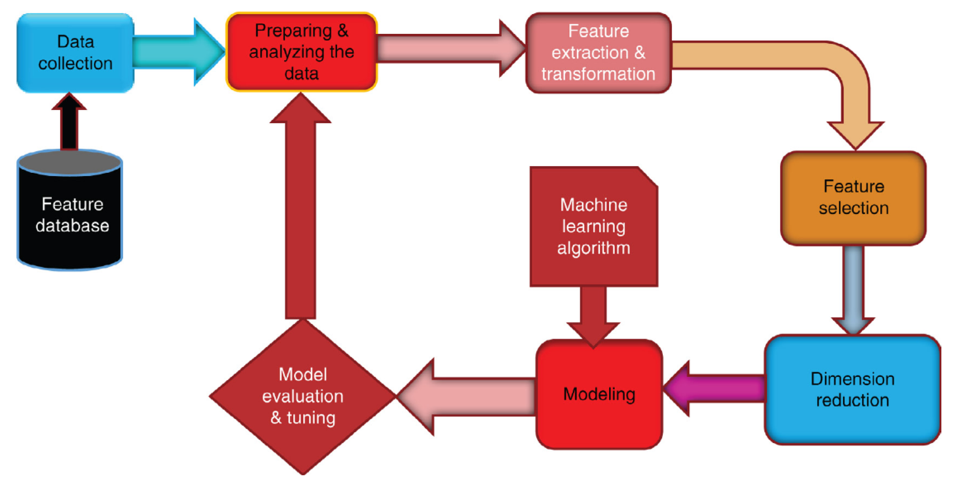
Machine learning approaches have been widely investigated for solving tasks in the wind energy sector, especially supervised learning, because the target variable to predict or classify depends strictly on the nature of a predefined input data [27]. The objective task of this research was also subjected to a supervised regression solution since here continuous numerical values are predicted from predefined data sets. These data samples are prepared and analyzed beforehand, the features are well-defined, and the labels/responses are already known in advance. Therefore, a supervised learning algorithm can construct relations and associations between the inputs and their corresponding outputs in the learning phase. Then, we can use those trained models to predict an output from unseen data.
The general procedure in a supervised learning task is presented in Figure 1. The methodology that rules our research is based on the Cross Industrial Standard Process for Data Mining, CRISP-DM [28] since it estimates, creates, evaluates, and redefines over and over, the machine learning system until getting a satisfactory result of the proposed models.
The models were trained using the same input data, taking special care in avoiding data-leakage in the train/split process. This allowed some observations of the advantages and disadvantages of each model for the first interactions. For subsequent model iteration, adjustments were made to the feature selections and their transformations to achieve the best results for each model. With this, we were able to identify the strengths of each model according to the training information and features used. The following algorithms were used to construct the models:
- Regression: Linear, Ridge, Lasso, and Elastic.
- Decision-making: Decision Trees (DT).
- Support vector machines: Support Vector Regression (SVR).
- Ensemble methods: Random Forest (RF).
A detailed theory related to these algorithms is available in [30].
These models were tested in three scenarios (refer to Section 2.3) in order to assess the performance, where they were subjected to different training sets. In the modeling process, several procedures were performed to reduce the uncertainties, such as data coverage, data quality, data imputation, time series analysis, statistical analysis, outliers analysis, feature engineering, hyperparameters tuning, cross-validation, and scoring evaluation. This process was carried out using the following libraries: Apache Spark [31], Scikit-learn [32], statsmodels [33], and pandas [34].
2.2. Training Data Sources
Two sources of data were available to train and assess the models. The first comes from a meteorological mast, henceforth named observed data, and the second one is modeled mesoscale data from the New European Wind Atlas (NEWA) [7], hereafter mesoscale data.
The observed data provided the following information: wind speed from a cup anemometer at , 75 and 50 ; wind direction at , and . Temperature at 100 , and 25 ; Pressure at ; Relative humidity at . This data set has a resolution of 10 min average for each variable, and the time frame was two years. The signals at 50 and 75 were used to calculate the resulting wind speed time series at a height of . The results of the ML models and the power-law method, were compared against the measured wind speed at .
The NEWA mesoscale data, for the same location as the observed data, provides time series for 23 climate signals [35]. However, some of them are not related to the horizontal wind speed because they are not physically related to the vertical fluxes of heat, moisture, momentum, or roughness of the Earth’s surface in any case [36]. Consequently, the best procedure was to discard those variables to avoid confusion in the models by giving information not related to the target feature. The variables listed in Table 1 were chosen and later studied to conclude whether those variables increase the model performance or not. The machine learning model for predicting wind speed is weather-dependent with seasonal variations. Therefore, the time frame of the data set should be sufficient to cover the seasonal variations: summer, winter, autumn, and spring.
2.3. Scenarios
Defining several scenarios brings the possibility to compare and analyze the cost/benefit of each model solution in terms of maintainability, computational demand, and accuracy [37]. The following scenarios allowed us to assess the performance of the seven models against the mesoscale data from the NEWA, the observed data from the met mast, and a combination of both.
- Scenario A: only mesoscale data is available to extrapolate the wind speed at 102 height.
- Scenario B: only observed data is available to extrapolate the wind speed at 102 height.
- Scenario C: observed, and mesoscale data are available to extrapolated wind speed at 102 height.
2.4. Assessment
The learning model performance evaluation is used to assess the target approximation’s quality that the model represents. It measures how close/far off the predicted values are versus the real values recorded by the met mast at a 102 m height. The following indicators were used to compare model performance (they were computed using 5 folds cross-validation). Explanations and significance for each metric are presented in Appendix B.
- Mean Absolute Error (MAE);
- Mean Squared Error (MSE);
- Root Mean Squared Error (RMSE);
- Coefficient of determination ().
3. Results
3.1. Scenario A: Extrapolate Wind Speed Using Mesoscale Data from Newa
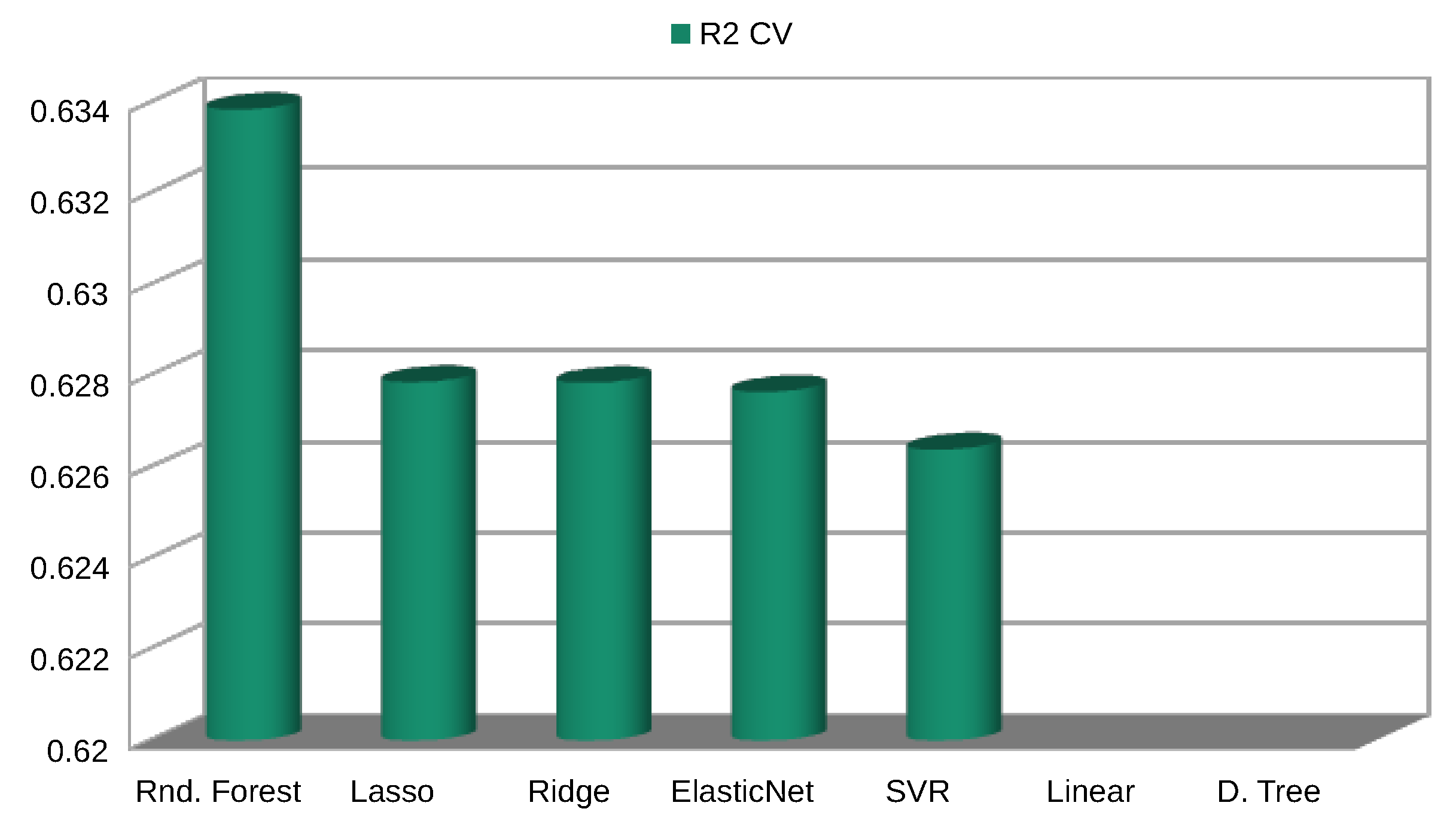
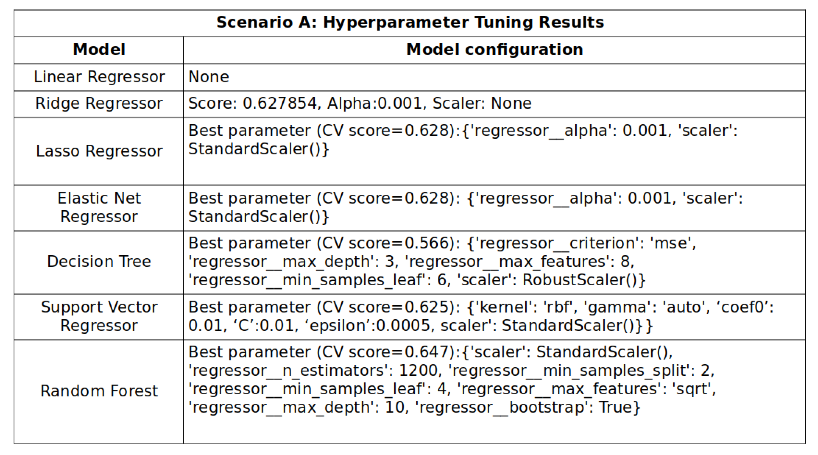
Statistical variables for assessing the models in this scenario are listed in Table 2, and their configurations in Figure A1. A graphical representation of the model’s errors and the model’s performance are presented in Figure 2 and Figure 3, respectively.
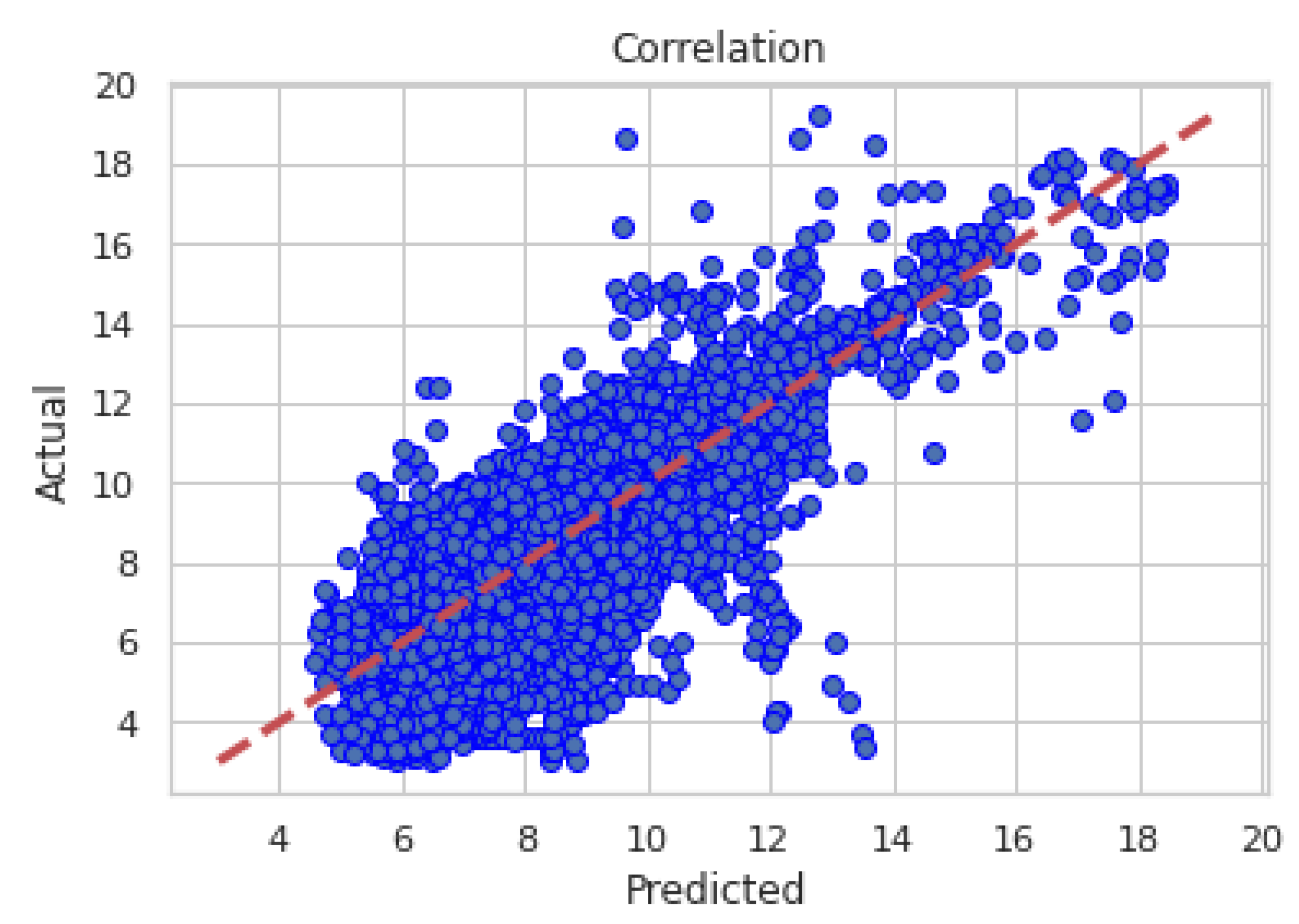
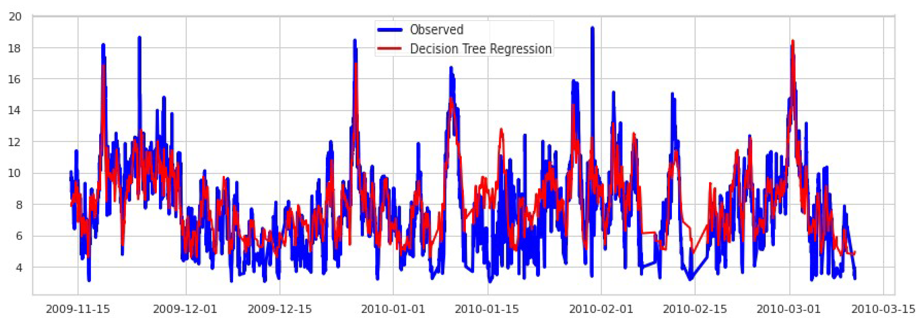
The best wind speed predictions, at the target height and using only mesoscale data, were obtained by the model based on a Random Forest. It substantially exceeds the predictions obtained by the other ML models, and the power law. The scores obtained by the RF were: . Additionally, the RF model was trained with the same information that the power law used, WS at 50 m, and 75 m height. It confirmed that the ML model is more robust than the power law, even when both models use the same available information. The metrics for the Power Law method are . Figure 4 shows the correlation of WS predicted by the RF with the data recorded by the met mast; Figure 5 shows an example of the RF predicted time series in a period of high variability of the wind speed.
3.2. Scenario B: Extrapolate Wind Speeds Using Data from a Met Mast
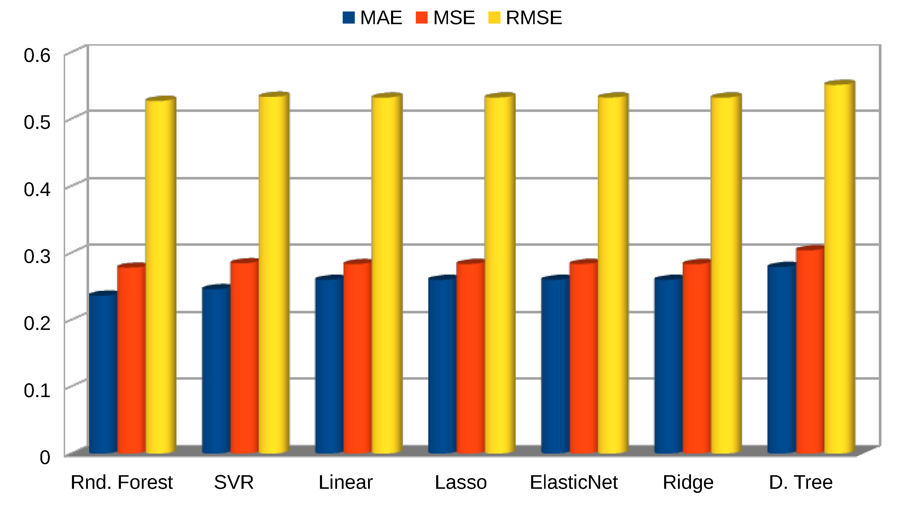
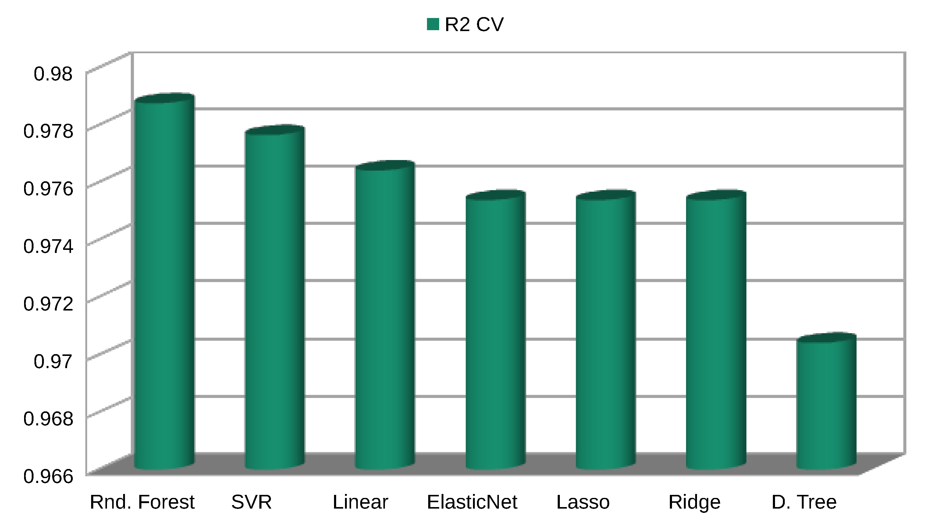
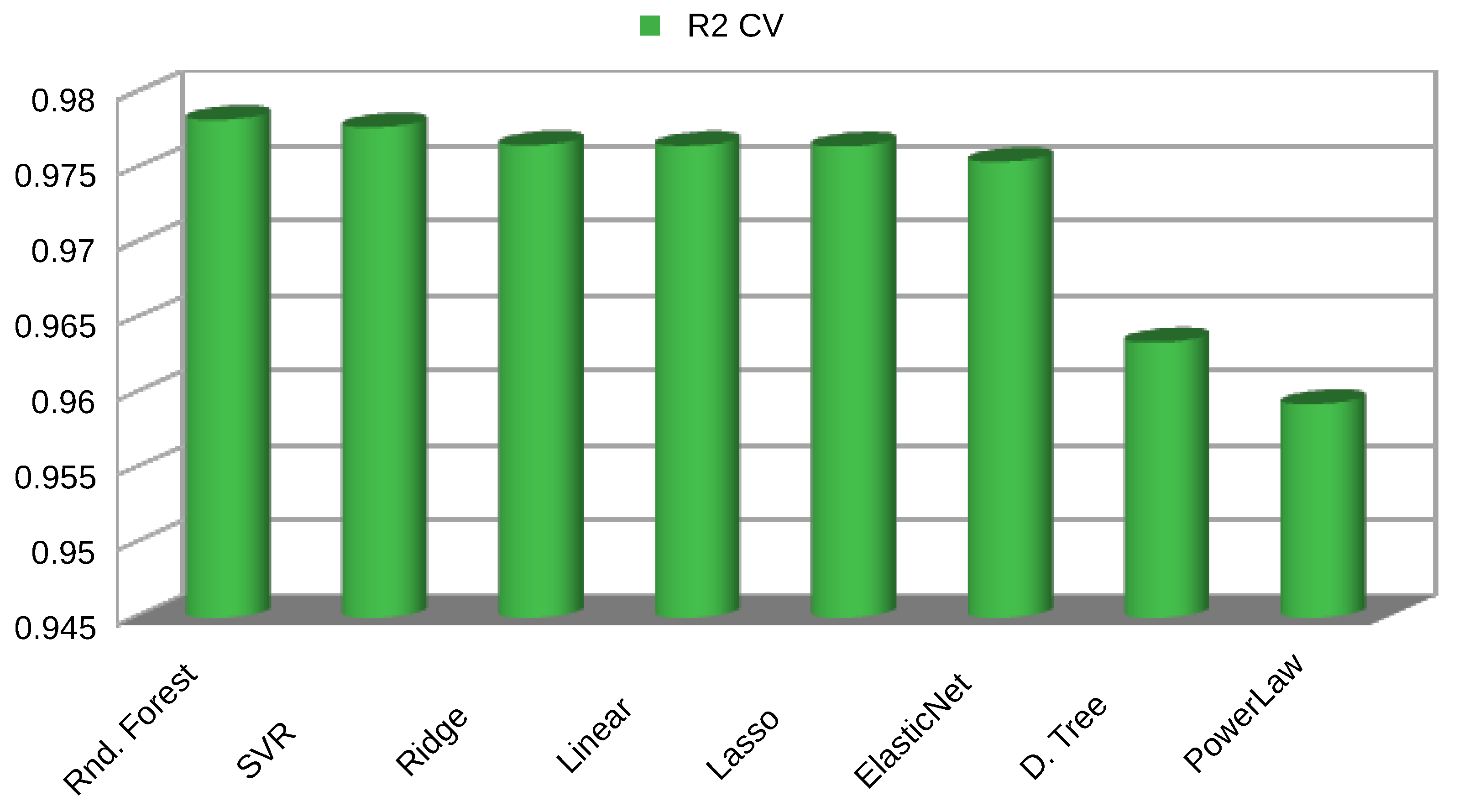
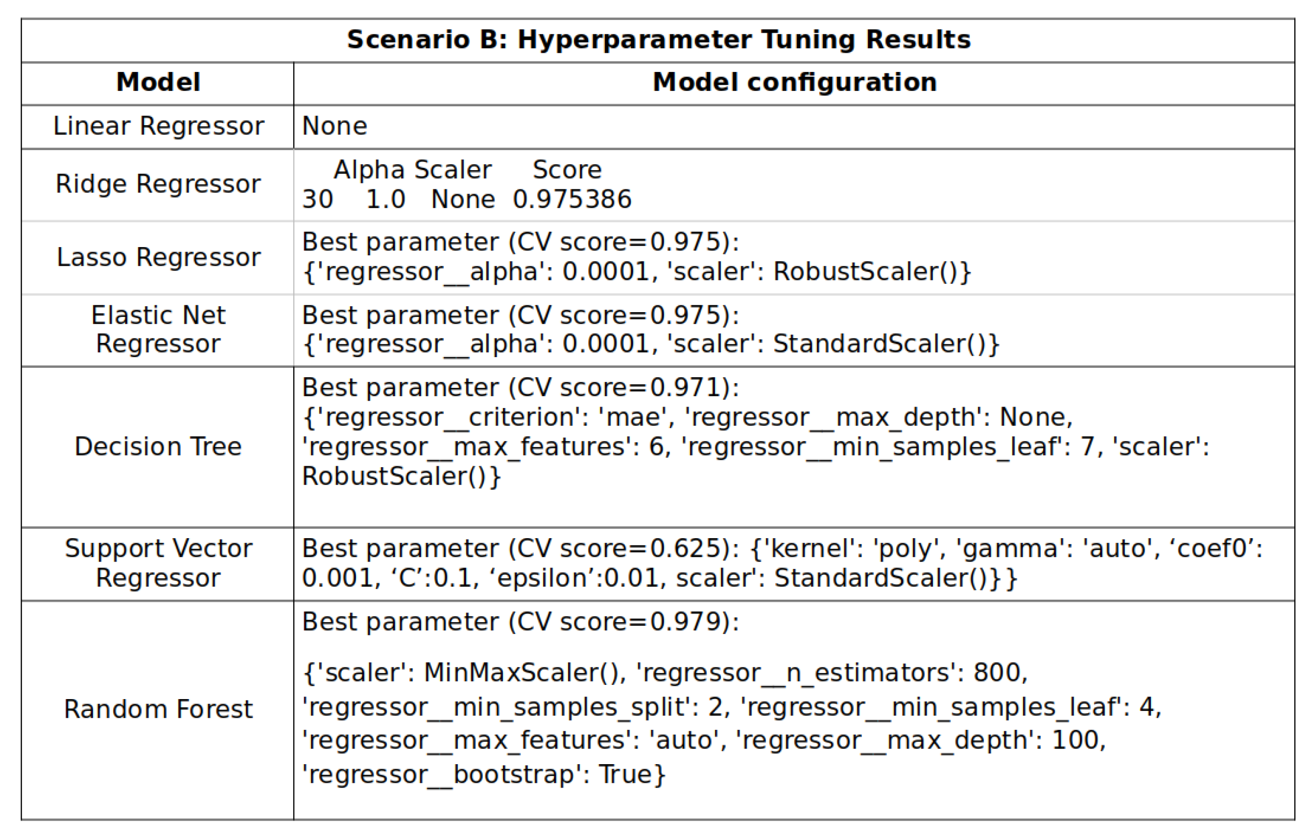
Statistical variables for assessing the models in this scenario are listed in Table 3, and their configurations in Figure A2. A graphical representation of the model’s errors and the model’s performance are presented in Figure 6 and Figure 7, respectively.
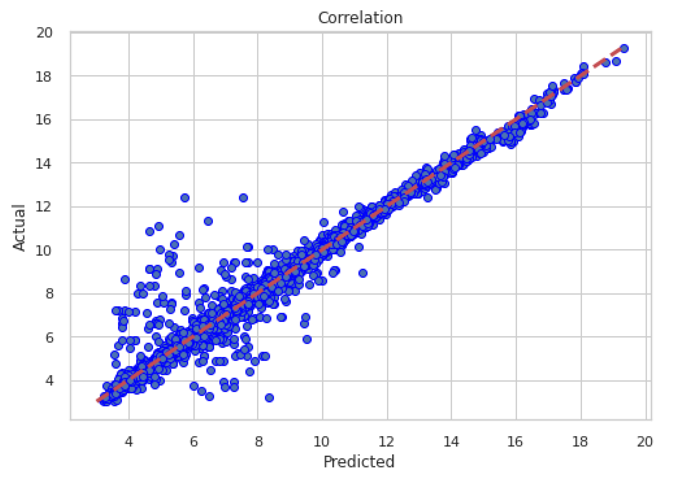
Similarly to Scenario A, the best model performances in terms of coefficient of correlation and errors, using only observed data during the training phase, was the Random Forest (RF), followed by the Support vector machine, and then by the Linear regression. The RF obtained a . All machine learning models outperformed the power law method, which metrics are . Figure 8 shows the correlation of WS predicted by the RF with the recorded by the met mast; Figure 9 shows an example of the RF predicted time series in a period of high variability of the wind speed.
3.3. Scenario C: Extrapolate Wind Speeds Using Data from a Met Mast and Mesoscale from the Newa
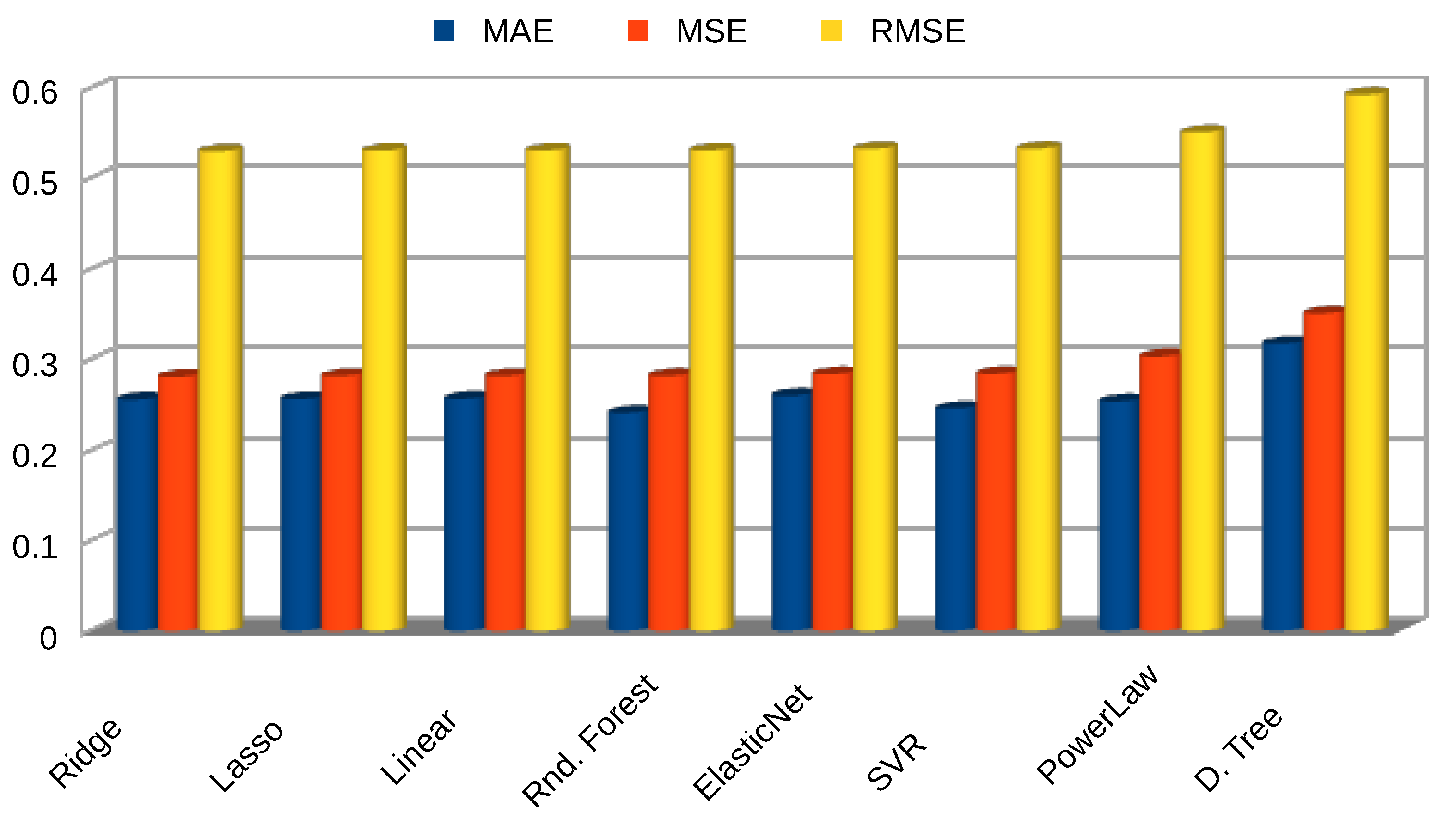
Statistical variables for assessing the models in this scenario are listed in Table 4, and their configurations in Figure A3. A graphical representation of the model’s errors and the model’s performance are presented in Figure 10 and Figure 11, respectively.
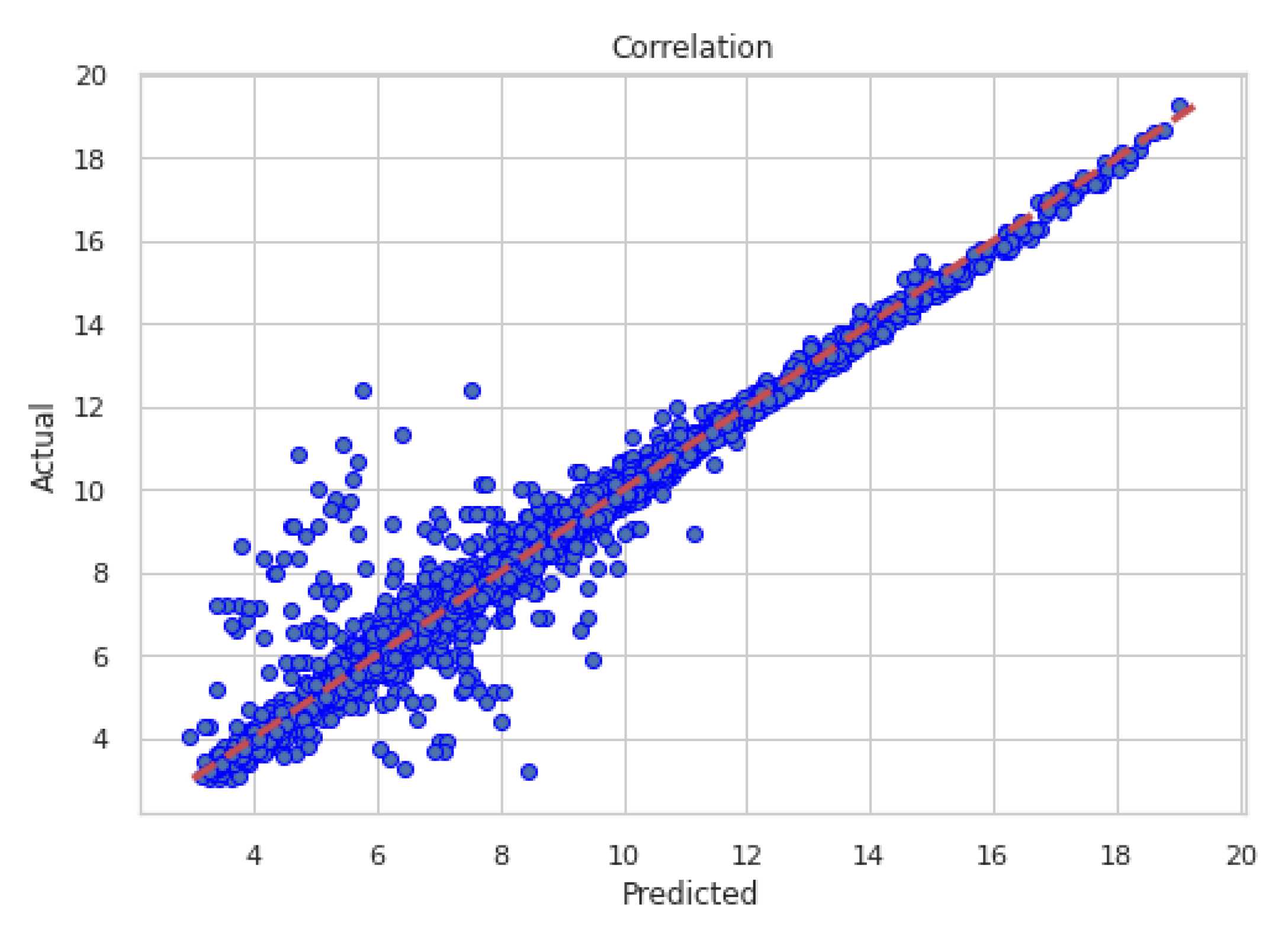
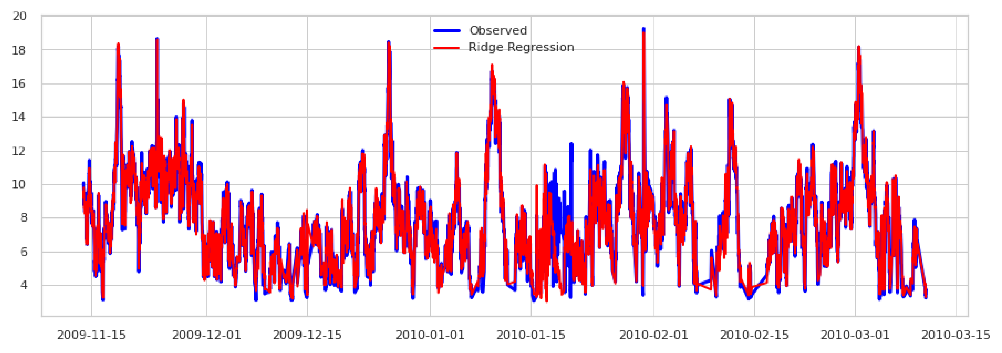
When the models are trained using all the information available from the mesoscale and observed datasets, the best results were obtained by the Random forest, followed by the support vector machine, and now in third place we have again a regression model, but this time not the linear one but the penalized Ridge regression. The RF model had a . As expected, all the ML models outperformed the power law method. Figure 12 shows the correlation of WS predicted by the Ridge regression with the recorded by the met mast; Figure 13 shows an example of the Ridge model predicted time series, in a period of high wind speed variability.
4. Discussion
4.1. Scenario A: Extrapolate Wind Speed Using Mesoscale Data from Newa
Based on the , the Decision Tree scored far below its peers. According to the literature, it was expected to obtain better results than the SVR. However, its performance is below all the linear regressions. The regressions models do not extract most features’ information; they focus the learning on only wind speeds. For the SVR, the kernel generated a hyperplane that contains above 62% of the attributes transformations. It is verified that the Decision tree cannot predict accurately since its MSE is very high, and only 40% of the variance in the WS 102 is collectively explained by its regression. However, when many decision trees are combined in a single model, which is known as a Random Forest (which belongs to the ML family of ensemble methods), the results obtained in terms of error and performance are much higher. In fact random forest gets the best score among all the methods. This is due to a wide range of decision paths are generated, which manage to include many more features of the training set, than when using a single decision tree.
After determining that RF was the best method for scenario A, it was compared against the power law method. In a first comparison, the Random forest was trained exclusively with the same mesoscale information that the power law method uses, that is, the wind speed at 50 m and the wind shear coefficient (using the wind speed at 75 m). In this case, the RF obtained an improvement of the of 33% compared to that obtained by the power law method. For a second comparison, a RF is trained again, but this time using all the information that the NEWA mesoscale model provides, mathematical and statistical transformations carried out in the featuring engineering process (which managed to relate the atmospheric variables, with their effects on wind speed), and an extensive hyperparameter tuning using parallel computing in Pyspark. As expected, by using all the information available from the NEWA mesoscale model, the R2 of the predictions was further improved in the wind extrapolation. In this case, the RF obtained an 42% better than that of the power law method, and 9% better than the obtained by the RF model used for the first comparison.
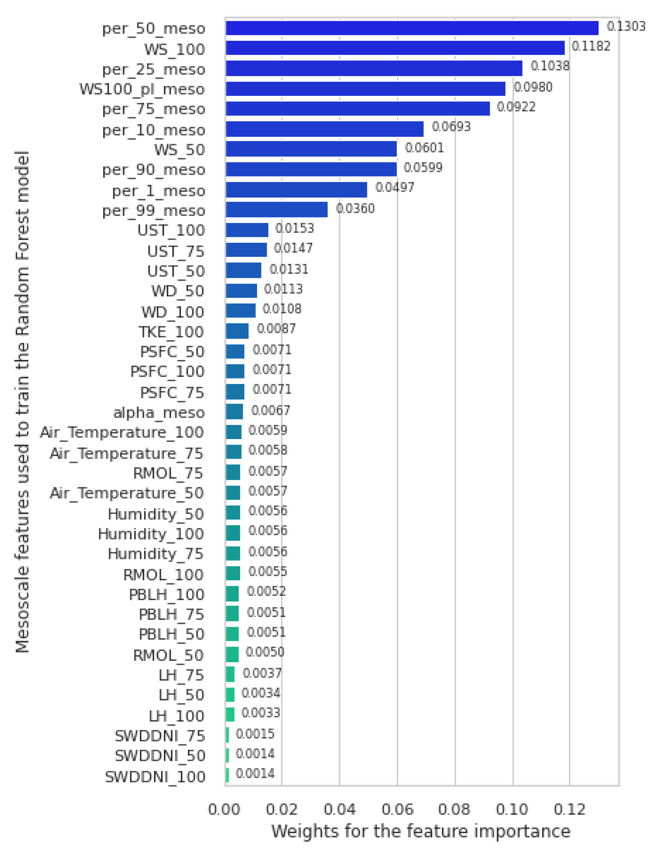
We rank the features’ contributions for the RF model that was trained with all the information from the NEWA mesoscale model (38 features in total) in Figure 14. The more outstanding ones come from statistical transformations. However, we noticed that the model takes information from all the features, which is the main advantage of the ML techniques over the power law method, where it can only use two wind speeds at different heights.
One advantage of the RF over other ML techniques is that it captures the non-linear features (avoid under-fitting). We can demonstrate this by having a normal distribution of the residuals and the feature utilization rank. The RF relies on a decision making process that accounts for every single possible combination among all the features. However, it explains why the RF model is as well the most expensive in computational terms.
4.2. Scenario B: Extrapolate Wind Speeds Using Data from a Met Mast
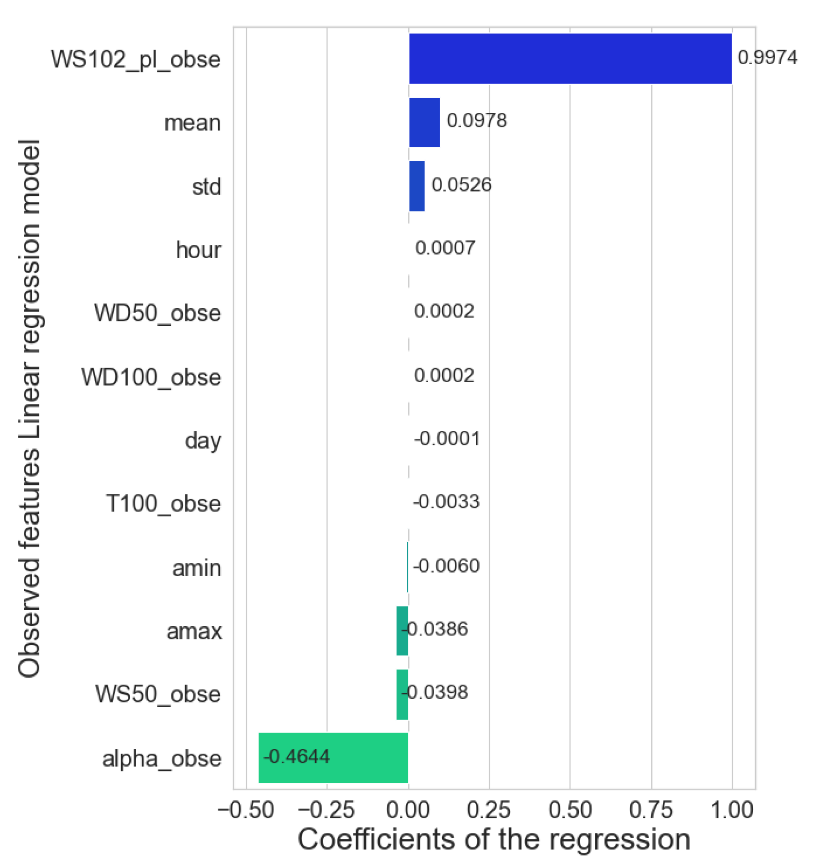
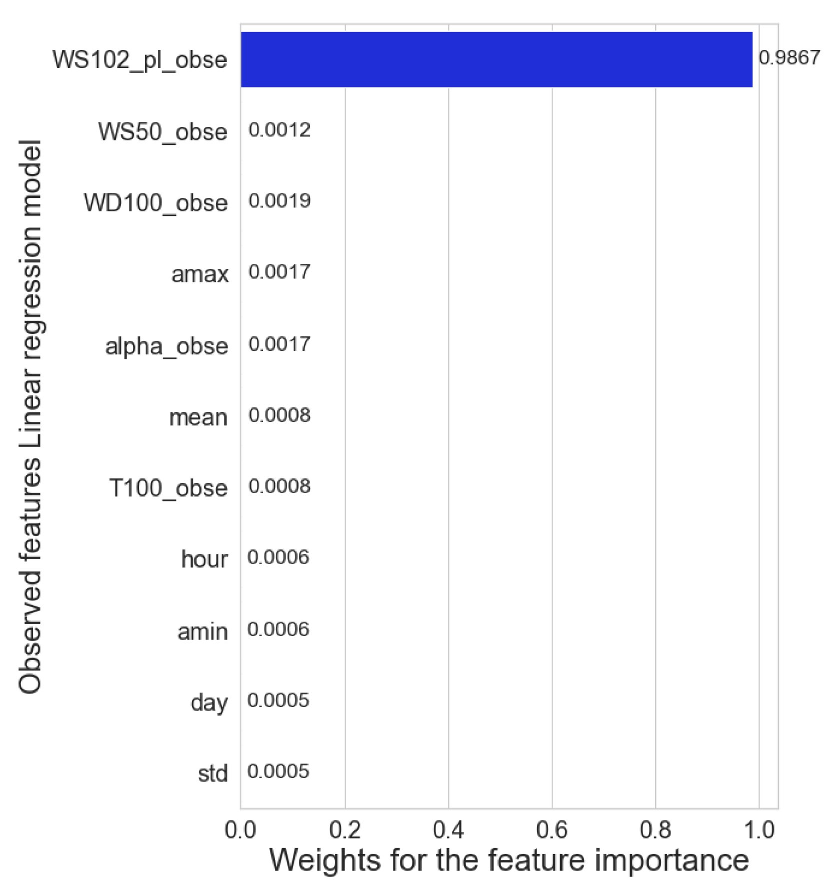
We can appreciate that the scores between the ML models do not differ significantly from each other in this scenario. Based on the , the decision tree still scored below its peers. Remarkably, with the observed data, the Linear regressor stands in third place from the best models. According to feature importance for linear regression in this scenario (Figure 15), the model learns directly from the power-law feature (that inherit the information from the wind speeds at 50 and 75 ), and the wind shear to make the predictions. This model also takes statistical features such as the mean and the standard deviation as secondary teachers. The supervisor model tended to take more statistical analysis along with the mathematical transformations. Surprisingly, the best score is obtained when the RF learned almost entirely (98%) from the power-law feature, leaving the remaining 2% among the other features (Figure 16). As a result, the ML model’s performance is similar to the traditional method. However, the ML models are still better because they correct some outliers that the power-law does not. The wind speeds predictions for all the models in the range of 4 to 10 deviate the most from reality. It was expected because the significant concentration of outliers in the data are in that range of high fluctuations that reflect the volatile nature of wind speed.
The Linear Regression model exceeds the quality of the Power Law predictions by 1.8% in the and is lower than RF by only 0.23%. The error analysis shows that the LR is just as robust as the RF to outliers and data with a high percentage of abrupt change. In computational costs, the RF is way more expensive than the LR. On average, the RF model requires 10 min to solve the task, while LR requires only 5 s. Additionally, the hyperparameter tuning for the RF model took 54 h using distributing computing on three CPUs with six cores each. The LR does not require hyperparameter tuning. Therefore, the recommended model for this scenario is the LR.
4.3. Scenario C: Extrapolate Wind Speeds Using Data from a Met Mast and Mesoscale from the NEWA
The ML models surpass the Power Law method as in the previous two scenarios. Among them, the best model performance belongs to the Random forest, followed by the support vector machine, and in third place, we have a penalized ridge regression. Not all the models benefited from the combination of met mast features and NEWA features, as is the case of Decision Tree, which decreased its by 0.7%, and Random Forest, which dropped by 0.059%. This can be explained by recognizing that the problem is largely solved with the features derived from the observed data. Additionally, adding more features to train the RF creates more branches, but in the end, the trees decided to go through one of the branches and end up in a leaf with a lower bias for the prediction, omitting most of the other branches. The models that benefited most in this scenario were the Ridge regression that increases its performance on by 0.19% and Lasso by 0.10%. For Elastic Net, linear regression and SVR, there was neither improvement nor degradation on the scores; they just omitted the NEWA features completely.
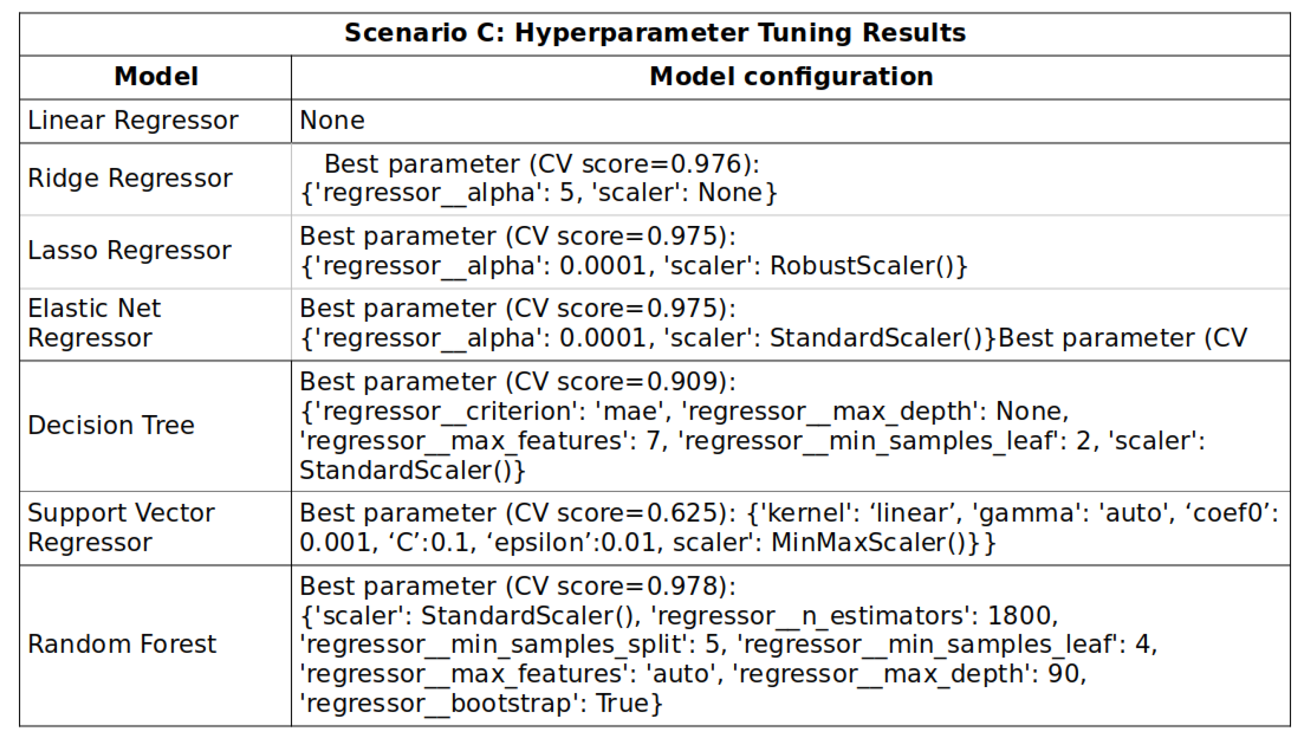
Using Grid Search CV in the ElasticNet model, the best value for alpha was found: 0.01. This means that the model was adjusted almost purely in a Ridge configuration penalized for L2 Norm. The RF scores in , 0.09% higher than the Ridge model, and the SVR only 0.012% more. At this scale, we can conclude that the SVR and the Ridge regressor have the same score. However, if we compare the MSE, the Ridge regressor outperforms all the others models. Comparing computational costs, the Ridge model took 2.28 s to solve the task; meanwhile, the RF and the SVR took almost 2 h. The GridSearch Cross-Validation for the RF and SVM was not carried because it exceeded three days of compilation time using a cluster with three distributed nodes. Based on the previous findings, the task for scenario C has to be solved by a Ridge regression since RF, and SVR models are too computationally expensive. Furthermore, they do not give any considerable improvement in the predictions. The features most studied by the Ridge model (Figure 17) in descending order were: mathematical transformations, power-law, wind shear, mesoscale WS at 100 m, air temperatures, WS observation at 50 m, humidity, Turbulent Kinetic Energy, and Friction Velocities at different heights.
5. Conclusions
Using several sources of information (as is the case when using mesoscale data) can lead to an imbalanced data set that is not useful for training an ML model. Therefore, a feature engineering process is required to derive valuable features from the NEWA mesocale and observed data. The mathematical transformation stands out in the feature importance for all three scenarios. The mathematical features link lower wind speeds, temperatures, humidities, and other climate variables well to the higher height objective variable. By training the model with these features, the model does not infer from scratch; on the contrary, it provides a solid base over other assumptions made by the models. A group of 33 features out of 69 are the most suitable to train the models, based on several trial and error experiments and an analysis of the relations between the features and the physical phenomena that rule the wind speed behavior. The 33 features are: seven come from the measured data, four are focused on temporal attributes, 20 come from the mesoscale model, and two are related to spatial characteristics.
In all the experiments, the machine learning methods trained with mesoscale data, observed data, or a combination of both are superior, as expected, to the power-law method in metrics such as the MAE, MSE, RMSE, and the . When modeled data is available, the predictions become more complex and should be used in an assembled model such as Random Forest (despite its expensive computational demands), which achieves an acceptable prediction. Moreover, when meteorological mast data is available, a regression model at a cheaper computational cost could achieve similar performance to the one conducted by the random forests. Linear regression proved particularly effective when predicting using only measured data, while the Ridge model performed best when mesoscale information is combined with observed data. It was demonstrated that the models depend entirely on how they are trained. The most crucial phase of the machine learning process is to guarantee success in the steps before the modeling phase, such as data cleaning, feature engineering, imputation methods, and construction of the training and evaluation sets. The best scenario result was obtained when mesoscale and observed data were used together. As a result, we obtain better model predictions because the model will use climate information, such as temperatures, humidity, pressures, friction velocities, and wind directions, among other variables.
This work opens possible avenues for new research. On the one hand, it would be essential to determine the level of confidence and uncertainty that a wind energy resource assessment would deliver if a machine learning method is used instead of the power law. More importantly, if an acceptable level of uncertainty is obtained when only modeled data is used. It could lead us in the future to determine if the measurement campaigns can be partially avoided or their costs reduced by not needing to use tall measurement towers. Additionally, an optimized mesoscale model with a coarse resolution could be used to determine if the ML models will assign a higher priority to the wind climate atmospheric conditions, which are, in the end, the direct drivers for the wind velocity, and improve in that way the predictions. Finally, ways to improve the model based on the Random Forest could be investigated, for example, using a high-performance computing platform, which allows a more extensive and precise hyperparameter tuning of the model. Using an HPC platform, one could also propose an ensemble model between the Random Forest and a neural network or a multi-gen genetic programming-based model to catch all the remaining relations between the target variable and the features the RF cannot describe.
Author Contributions
Conceptualization L.B., P.L. and H.T.; methodology, L.B. and H.T.; software, L.B.; validation, L.B.; formal analysis, L.B.; investigation, L.B.; resources, L.B. and P.L.; data curation, L.B.; writing—original draft preparation, L.B.; writing—review and editing, H.T.; visualization, L.B.; supervision, H.T.; project administration, P.L.; funding acquisition, P.L. All authors have read and agreed to the published version of the manuscript.
Funding
This research was funded by and innovation project of the company DNV—Energy Systems, Northern Europe.
Institutional Review Board Statement
Not applicable.
Informed Consent Statement
Not applicable.
Data Availability Statement
Not applicable.
Acknowledgments
To DNV—Energy Systems—Germany, and the University of Oldenburg, for financing and supporting this research. Additionally, a recognition to the people who developed and maintained the software used in the models: Scikit-Learn, PySpark, Pandas, Matplotlib, and Python.
Conflicts of Interest
The authors declare no conflict of interest.
Abbreviations
| AI | Artificial Intelligence |
| ANN | Artificial Neural Network |
| CRISP-DM | Cross Industrial Standard Process For Data Mining |
| CV | Cross-Validation |
| DNN | Deep Neural Network |
| DT | Decision Trees |
| LR | Linear Regression |
| RG | Ridge Regression |
| MAE | Mean Absolute Error |
| MAPE | Mean Absolute Percent Error |
| ML | Machine Learning |
| MSE | Mean Square Error |
| NaN | Not a Number Value |
| NEWA | New European Wind Atlas |
| OLS | Ordinary Least Squares |
| PBLH | Planetary Boundary Layer Height |
| Probability Density Function | |
| RF | Random Forest |
| RMSE | Root Mean Square Error |
| SVM | Support Vector Machine |
| WPD | Wind Power Density |
| WRF | Weather Research Forecasting model |
| WS | Wind Speed |
Appendix A. Ml Models Configuration
The following tables present the configuration of the machine learning algorithms that best performed in the cross validation test for each of the three scenarios proposed in Section 2.3.
Figure A1.
Hyperparameter configuration for the models of Scenario A.

Figure A2.
Hyperparameter configuration for the models of Scenario B.

Figure A3.
Hyperparameter configuration for the models of Scenario C.

Appendix B. Performance Metrics
The indicators that can be used to compare model performance in regression tasks are presented to continue. For the final evaluation of the , a cross-validation with 5 folds was used. There, N represents the total number of data points, y the actual value, the predicted value, is the residual, and is the mean of the observed data denoted by .
Mean Absolute Error (MAE): It asses the absolute differences, and is less sensitive to outliers. Thus, it is good for comparing different models.
Mean squared error (MSE): It is the average of the squared differences. Even the small errors are penalized. It can lead to an over-estimation of how bad the model is. MSE is used to determine the extent to which the model fits the data.
Root Mean Squared Error (RMSE): It is the standard deviation of the residuals. It has a high penalty on large errors (the errors are first squared before averaging); thus, it is used when avoiding bigger errors is desirable.
Coefficient of determination (): It compares the regression model with a constant baseline and tells us how much our model differs from the original one. It is related to the correlation coefficient, r, which tells you how strong of a linear relationship there is between two variables.
References
- International Renewable Energy Agency. Capacity Statistics 2019; Technical Report; IRENA: Abu Dhabi, United Arab Emirates, 2020. [Google Scholar]
- International Renewable Energy Agency. Future of Wind 2019; Technical Report; IRENA: Abu Dhabi, United Arab Emirates, 2020. [Google Scholar]
- Roeth, J. Wind Resource Assessment Handbook; AWS Truepower: New York, NY, USA, 2010. [Google Scholar]
- Gasch, R.; Twele, J. (Eds.) Wind Power Plants: Fundamentals, Design, Construction and Operation; Springer: Berlin/Heidelberg, Germany, 2012. [Google Scholar] [CrossRef]
- Valsaraj, P.; Drisya, G.V.; Kumar, K.S. A Novel Approach for the Extrapolation of Wind Speed Time Series to Higher Altitude Using Machine Learning Model. In Proceedings of the 2018 International CET Conference on Control, Communication, and Computing (IC4), Thiruvananthapuram, India, 5–7 July 2018; pp. 112–115. [Google Scholar] [CrossRef]
- Mohandes, M.A.; Rehman, S. Wind Speed Extrapolation Using Machine Learning Methods and LiDAR Measurements. IEEE Access 2018, 6, 77634–77642. [Google Scholar] [CrossRef]
- Europe Union. The New European Wind Atlas (NEWA); Geoscientific Model Development: Munich, Germany, 2020. [Google Scholar]
- Manwell, J.F. Wind Energy Explained: Theory, Design and Application; Wiley: Hoboken, NJ, USA, 2009. [Google Scholar]
- Eyecioglu, O.; Hangun, B.; Kayisli, K.; Yesilbudak, M. Performance comparison of different machine learning algorithms on the prediction of wind turbine power generation. In Proceedings of the 8th International Conference on Renewable Energy Research and Applications, ICRERA 2019, Brasov, Romania, 3–6 November 2019; pp. 922–926. [Google Scholar] [CrossRef]
- Malakhov, A.; Goncharov, F. Testing proaches for wind plants power output. In Proceedings of the 2019 International Youth Conference on Radio Electronics, Electrical and Power Engineering (REEPE), Moscow, Russia, 14–15 March 2019. [Google Scholar] [CrossRef]
- Liu, Y.; Zhang, H. An Empirical Study on Machine Learning Models for Wind Power Predictions. In Proceedings of the 2016 15th IEEE International Conference on Machine Learning and Applications (ICMLA), Anaheim, CA, USA, 18–20 December 2017; pp. 758–763. [Google Scholar] [CrossRef]
- Ji, G.R.; Han, P.; Zhai, Y.J. Wind speed forecasting based on support vector machine with forecasting error estimation. In Proceedings of the Sixth International Conference on Machine Learning and Cybernetics, ICMLC 2007, Hong Kong, China, 19–22 August 2007; Volume 5, pp. 2735–2739. [Google Scholar] [CrossRef]
- Brahimi, T. Using artificial intelligence to predict wind speed for energy application in Saudi Arabia. Energies 2019, 12, 4669. [Google Scholar] [CrossRef] [Green Version]
- Liu, Y.; Wang, J.; Collett, I.; Morton, Y.J. A Machine Learning Framework for Real Data Gnss-R Wind Speed Retrieval. In Proceedings of the IGARSS 2019—2019 IEEE International Geoscience and Remote Sensing Symposium, Yokohama, Japan, 28 July–2 August 2019; pp. 8707–8710. [Google Scholar] [CrossRef]
- Ali, M.E.K.; Hassan, M.Z.; Ali, A.B.; Kumar, J. Prediction of Wind Speed Using Real Data: An Analysis of Statistical Machine Learning Techniques. In Proceedings of the 2017 4th Asia-Pacific World Congress on Computer Science and Engineering, APWC on CSE 2017, Mana Island, Fiji, 11–13 December 2017; pp. 259–264. [Google Scholar] [CrossRef]
- Ak, R.; Fink, O.; Zio, E. Two Machine Learning Approaches for Short-Term Wind Speed Time-Series Prediction. IEEE Trans. Neural Netw. Learn. Syst. 2016, 27, 1734–1747. [Google Scholar] [CrossRef] [PubMed]
- Albrecht, C.; Klesitz, M. Long-term correlation of wind measurements using neural networks: A new method for post-processing short-time measurement data. In Proceedings of the European Wind Energy Conference and Exhibition 2007, EWEC 2007, Milan, Italy, 7–10 May 2007; Volume 2, pp. 755–762. [Google Scholar]
- Cheggaga, N.; Ettoumi, F.Y. A Neural Network Solution for Extrapolation of Wind Speeds at Heights Ranging for Improving the Estimation of Wind Producible. Wind. Eng. 2011, 35, 33–53. [Google Scholar] [CrossRef]
- Türkan, Y.S.; Yumurtacı Aydoğmuş, H.; Erdal, H. The prediction of the wind speed at different heights by machine learning methods. Int. J. Optim. Control. Theor. Appl. 2016, 6, 179. [Google Scholar] [CrossRef]
- Cheggaga, N. A new artificial neural network–power law model for vertical wind speed extrapolation for improving wind resource assessment. Wind. Eng. 2018, 42, 510–522. [Google Scholar] [CrossRef]
- Vassallo, D.; Krishnamurthy, R.; Fernando, H.J.S. Decreasing wind speed extrapolation error via domain-specific feature extraction and selection. Wind. Energy Sci. 2020, 5, 959–975. [Google Scholar] [CrossRef]
- Bodini, N.; Optis, M. How accurate is a machine learning-based wind speed extrapolation under a round-robin approach? J. Phys. Conf. Ser. 2020, 1618, 062037. [Google Scholar] [CrossRef]
- Adli, F.; Cheggaga, N.; Farouk, H. Vertical wind speed extrapolation: Modelling using a response surface methodology (RSM) based on unconventional designs. Wind. Eng. 2022, 35, 33–53. [Google Scholar] [CrossRef]
- Emeksiz, C. Multi-gen genetic programming based improved innovative model for extrapolation of wind data at high altitudes, case study: Turkey. Comput. Electr. Eng. 2022, 100, 107966. [Google Scholar] [CrossRef]
- Shi, T.; He, G.; Mu, Y. Random Forest Algorithm Based on Genetic Algorithm Optimization for Property-Related Crime Prediction. In Proceedings of the 2019 International Conference on Computer, Network, Communication and Information Systems (CNCI 2019), Qingdao, China, 27–29 March 2019; Atlantis Press: Amsterdam, The Netherlands, 2019; pp. 526–531. [Google Scholar] [CrossRef] [Green Version]
- Farooq, F.; Nasir Amin, M.; Khan, K.; Rehan Sadiq, M.; Faisal Javed, M.; Aslam, F.; Alyousef, R. A Comparative Study of Random Forest and Genetic Engineering Programming for the Prediction of Compressive Strength of High Strength Concrete (HSC). Appl. Sci. 2020, 10, 7330. [Google Scholar] [CrossRef]
- Feng, J. Artificial Intelligence for Wind Energy. In A State of the Art Report 978-87-93549-48-7; DTU Wind Energy: Lyngby, Denmark, 2019. [Google Scholar]
- Chapman, P.; Clinton, J.; Kerber, R.Y.; Shearer, C.; Khabaza, T. CRISP-DM 1.0. Step-by-Step Data Mining Guide; SPSS Inc.: Chicago, IL, USA, 2000. [Google Scholar]
- Subasi, A. Practical Machine Learning for Data Analysis Using Python; Elsevier: Amsterdam, The Netherlands, 2020. [Google Scholar] [CrossRef]
- Baquero, L. Extraction of Section 2.5 from the Thesis Book: Theory about Machine Learning Used in This Research; ResearchGate: Berlin, Germany, 2022; Volume 1, pp. 25–36. [Google Scholar]
- Zaharia, M.; Xin, R.S.; Wendell, P.; Das, T.; Armbrust, M.; Dave, A.; Meng, X.; Rosen, J.; Venkataraman, S.; Franklin, M.J.; et al. Apache spark: A unified engine for big data processing. Commun. ACM 2016, 59, 56–65. [Google Scholar] [CrossRef]
- Pedregosa, F.; Varoquaux, G.; Gramfort, A.; Michel, V.; Thirion, B.; Grisel, O.; Blondel, M.; Prettenhofer, P.; Weiss, R.; Dubourg, V.; et al. Scikit-learn: Machine learning in Python. J. Mach. Learn. Res. 2011, 12, 2825–2830. [Google Scholar]
- Seabold, S.; Perktold, J. Statsmodels: Econometric and statistical modeling with python. In Proceedings of the 9th Python in Science Conference, Austin, TX, USA, 28 June–3 July 2010. [Google Scholar]
- McKinney, W. Data structures for statistical computing in python. In Proceedings of the 9th Python in Science Conference, Austin, TX, USA, 28 June–3 July 2010; Volume 445, pp. 51–56. [Google Scholar]
- Hahmann, A.N.; Sile, T.; Witha, B.; Davis, N.N.; Dörenkämper, M.; Ezber, Y.; García-Bustamante, E.; González Rouco, J.F.; Navarro, J.; Olsen, B.T.; et al. The Making of the New European Wind Atlas, Part 1: Model Sensitivity; Technical Report; Model Sensitivity; Geoscientific Model Development: Munich, Germany, 2020. [Google Scholar] [CrossRef] [Green Version]
- Camuffo, D. Microclimate for Cultural Heritage: Conservation, Restoration, and Maintenance of Indoor and Outdoor Monuments, 2nd ed.; Elsevier: Amsterdam, The Netherland; Boston, MA, USA, 2014. [Google Scholar]
- DNV GL. Framework for Assurance of Data Driven Algorithms and Models; DNV GL: Oslo, Norway, 2020. [Google Scholar]
Figure 1.
Supervised machine learning framework [29].
Figure 1.
Supervised machine learning framework [29].

Figure 2.
Model errors [].

Figure 3.
Performance scores.

Figure 4.
Correlation between observed (measured) data and results from the RF trained only with mesoscale data in .
Figure 4.
Correlation between observed (measured) data and results from the RF trained only with mesoscale data in .

Figure 5.
Observed and predicted wind speeds using RF based only in mesoscale data in .

Figure 6.
Model errors [].

Figure 7.
Performance scores.

Figure 8.
Correlation between observed (measured) data and results from the RF trained only with observed data in .
Figure 8.
Correlation between observed (measured) data and results from the RF trained only with observed data in .

Figure 9.
Observed and predicted wind speeds using the RF based only in mesoscale data in .

Figure 10.
Model errors [].

Figure 11.
Performance scores.

Figure 12.
Correlation of the Ridge regression predictions in .

Figure 13.
Wind speeds prediction from the Ridge regression using mesoscale and observed data. The units are in .
Figure 13.
Wind speeds prediction from the Ridge regression using mesoscale and observed data. The units are in .

Figure 14.
Feature importance for the best model in Scenario A: the random forest. Only mesoscale data for the model training. The sum of all the weights is one.
Figure 14.
Feature importance for the best model in Scenario A: the random forest. Only mesoscale data for the model training. The sum of all the weights is one.

Figure 15.
Feature importance for linear regression in Scenario B.

Figure 16.
Feature importance for Random Forest in Scenario B.

Figure 17.
Feature importance for the ridge regression in Scenario C.


Table 1.
Selected features from the mesoscale data.
| Item | Variable Name | Units | Nomenclature |
|---|---|---|---|
| 1 | Wind speed | WS | |
| 2 | Wind Direcction | WD | |
| 3 | Air Temperature | T | |
| 4 | Friction velocity | UST | |
| 5 | Shortwave direct normal radiation | SWDDNI | |
| 6 | Shortwave diffuse incident radiation | SWDDRI | |
| 7 | Inverse Obukhov length | RMOL | |
| 8 | Planetary boundary layer height | PBLH | |
| 9 | Surface pressure | PSFC | |
| 10 | Surface latent Heat Flux | LH | |
| 11 | Water vapour mixing ratio | QVAPOR | |
| 12 | Turbulent kinetic energy | TKE |
Table 2.
Results of the models when they are trained with NEWA mesoscale data.
| Model | MAE | MSE | RMSE | CV |
|---|---|---|---|---|
| Linear | 1.288161 | 2.907878 | 1.70525 | 0.626386 |
| Ridge | 1.274707 | 2.86232 | 1.691839 | 0.627854 |
| Lasso | 1.273021 | 2.853636 | 1.689271 | 0.62787 |
| ElasticNet | 1.271784 | 2.846432 | 1.687137 | 0.627652 |
| Desicion Tree | 1.565074 | 4.166773 | 2.041268 | 0.408519 |
| SVR | 1.288161 | 2.907878 | 1.70525 | 0.626386 |
| Random Forest | 1.269825 | 2.819217 | 1.679052 | 0.633857 |
Table 3.
Results of the models when they are trained with measured data.
| Model | MAE | MSE | RMSE | CV |
|---|---|---|---|---|
| Linear | 0.259943 | 0.283292 | 0.532251 | 0.97642 |
| Ridge | 0.259976 | 0.283458 | 0.532408 | 0.975386 |
| Lasso | 0.25996 | 0.283632 | 0.532571 | 0.975386 |
| ElasticNet | 0.259969 | 0.283562 | 0.532505 | 0.975386 |
| D. Tree | 0.279097 | 0.304115 | 0.551466 | 0.970416 |
| SVR | 0.24582 | 0.284564 | 0.533445 | 0.977656 |
| Rnd. Forest | 0.236336 | 0.278178 | 0.527425 | 0.97876 |
Table 4.
Results of the models when they are trained with mesoscale and observed data.
| Model | MAE | MSE | RMSE | CV |
|---|---|---|---|---|
| Linear | 0.256397 | 0.281716 | 0.530769 | 0.976455 |
| Ridge | 0.255516 | 0.280674 | 0.529786 | 0.976485 |
| Lasso | 0.256068 | 0.281552 | 0.530615 | 0.976416 |
| ElasticNet | 0.259969 | 0.283562 | 0.532505 | 0.975386 |
| D. Tree | 0.317277 | 0.3508 | 0.592284 | 0.963366 |
| SVR | 0.245733 | 0.283928 | 0.532849 | 0.977686 |
| Rnd. Forest | 0.240971 | 0.281742 | 0.530794 | 0.978178 |
Publisher’s Note: MDPI stays neutral with regard to jurisdictional claims in published maps and institutional affiliations. |
© 2022 by the authors. Licensee MDPI, Basel, Switzerland. This article is an open access article distributed under the terms and conditions of the Creative Commons Attribution (CC BY) license (https://creativecommons.org/licenses/by/4.0/).
Share and Cite
MDPI and ACS Style
Baquero, L.; Torio, H.; Leask, P. Machine Learning Algorithms for Vertical Wind Speed Data Extrapolation: Comparison and Performance Using Mesoscale and Measured Site Data. Energies 2022, 15, 5518. https://doi.org/10.3390/en15155518
AMA Style
Baquero L, Torio H, Leask P. Machine Learning Algorithms for Vertical Wind Speed Data Extrapolation: Comparison and Performance Using Mesoscale and Measured Site Data. Energies. 2022; 15(15):5518. https://doi.org/10.3390/en15155518
Chicago/Turabian StyleBaquero, Luis, Herena Torio, and Paul Leask. 2022. "Machine Learning Algorithms for Vertical Wind Speed Data Extrapolation: Comparison and Performance Using Mesoscale and Measured Site Data" Energies 15, no. 15: 5518. https://doi.org/10.3390/en15155518
Note that from the first issue of 2016, this journal uses article numbers instead of page numbers. See further details here.