Fault Diagnosis of Coal Mill Based on Kernel Extreme Learning Machine with Variational Model Feature Extraction

Abstract

Aiming at the typical faults in the coal mills operation process, the kernel extreme learning machine diagnosis model based on variational model feature extraction and kernel principal component analysis is offered. Firstly, the collected signals of vibration and loading force, corresponding to typical faults of coal mill, are decomposed by variational model decomposition, and the intrinsic model functions at different scales are obtained. Then, the eigenvectors consisting of feature energy and sample entropy in these functions are respectively calculated, and the kernel principal component analysis is used for noise removal and dimensionality reduction. Finally, the kernel extreme learning machine model is trained and tested with the dimension reduced feature vector as input and the corresponding coal mill state as output. The results show that the variational model decomposition extraction can improve the input features of the model compared with the single eigenvector model, and the kernel principal component analysis method can significantly reduce the information redundancy and the correlation of eigenvectors, which can effectively save time and cost, and improve the prediction performance of the model to some extent. The establishment of this model provides a new idea for the study of coal mill fault diagnosis.

1. Introduction

Coal mills are important equipment of the coal pulverizing system. The structure of the MPS medium-speed coal mill is shown in Figure 1 [1]. As can be seen from Figure 1, the raw coal entering the coal mill through the coal falling pipe is squeezed and ground by the grinding disc and the drum to become pulverized coal and then dried and carried into the separator by the primary air entering from the air ring around the grinding disc. In the separator, due to centrifugal force and inertial force, the qualified pulverized coal will be sent to the furnace for combustion, while the large particle pulverized coal will fall back into the grinding disc for re-grinding.

The coal mill faults, such as abnormal loading and mill vibration, etc., increase the unit consumption of coal pulverizing, and the output of grinding coal can not be guaranteed, which has a negative influence on the operation of the pulverizing system [1]. Therefore, the real-time monitoring and efficient diagnosis of the operation of the coal mill is of great significance to the safety and economical operation of the unit.

Generally, the complex field production environment causes that the measured signals contain certain random signals, and consequently, the feature extraction of signals is difficult. Therefore, how to realize the accurate extraction of signal features becomes the key to coal mill fault diagnosis. Gao et al., proposed a fault diagnosis method for coal mill system that can simulate fault samples to effectively solve the problem of fault sample collection [2]; Zhu et al., proposed an HP mill fault state recognition method based on the Gaussian regression model in combination with the HP mill fault diagnosis database, which plays a significant role in equipment fault diagnosis [3]; Vedika et al., mentioned a dynamic mathematical model, which can simulate the operation of coal mill under different operation conditions. The residuals generated by the fuzzy logic evaluation model are used to identify the type and degree of faults, which can realize the online monitoring and diagnosis of the major faults in the coal mill system [4]. Fan et al., designed a knowledge-based fine-grained coal mill operator support/control system for coal plants. The system is composed of mathematical coal mill model and expert knowledge database and has the ability of parameter estimation, coal mill performance monitoring, fault diagnosis and prediction, early warning and problem solving [5]. Wang et al., based on the coal mill model developed by Wei et al., proposed a method to monitor the state of the coal mill by identifying abnormal changes of model parameters [6,7,8,9]. Su et al., designed a system that uses wavelet analysis to record vibration signals and convert them into energy amplitudes. Through the analysis of these vibration characteristics and the estimation of the coal level of the mill, various operating problems such as overload and lack of coal are determined [10]. Emilija et al., proposed a method to detect mill wear and find the appropriate time to replace mill parts by using a multivariable control diagram to detect the spectral components of acoustic signals [11].

However, recent studies have found that the signal represented by the vibration of coal mill often has nonlinear and unsteady characteristics. When conventional means such as wavelet decomposition [12] and Fourier transform [13] are used for processing, it is difficult to extract the effective characteristics of the signal, thus affecting the diagnosis and classification accuracy of coal mill faults. Therefore, Huang et al., proposed and developed an empirical model decomposition algorithm, which has great advantages in processing nonlinear/steady signals and has been widely used [14]. However, due to the repeated application of cubic spline interpolation, this decomposition method is easy to cause the distortion of signal endpoint position (endpoint effect), which reduces the accuracy of signal decomposition. By transforming the model estimation into the solution of the variational problem, the variational model decomposition algorithm can effectively reduce the estimation error of the envelope caused by continuous accumulation and avoid model aliasing and endpoint effect [15]. Therefore, in this paper, the variational model decomposition algorithm is used to decompose the intrinsic model function (IMF) of the signal under different fault states, and the characteristic energy and sample entropy are calculated respectively to form multi-feature vectors, which can reflect the signal characteristics more comprehensively than a single feature quantity and are used as the input of the diagnostic model.

Generally, there is a certain linear correlation among variables in the feature vectors, and the feature vectors in some dimensions are not important, which increases the calculation cost and reduces the prediction accuracy of the model. Therefore, some scholars adopted principal component analysis (PCA) to achieve dimension reduction of feature vectors [16,17]. However, the relationship of traditional principal component analysis is linear, which leads to the poor applicability of nonlinear features. This reduces the classification accuracy, so it is particularly important to achieve nonlinear data analysis. The dynamic, recursive, moving window and multiple-model PCA variants are originated from process dynamics and non-stationarities with a paid cost of increased complexity [17]. The kernel principal component analysis (KPCA) realizes the extraction of nonlinear features by mapping the sample set of measurement space to high-dimensional space and has certain applications in fault diagnosis and other aspects [18]. In this paper, the KPCA is used to extract the reduced and effective features of feature vectors.

With the rapid development of artificial intelligence technology, neural network has attracted the attention and research of many scholars due to its advantages of strong nonlinear mapping ability and good learning effect [19,20]. Among them, the extreme Learning Machine (ELM) algorithm only needs to input the hidden layer weight and node bias randomly and can obtain the output weight by a simple calculation. With the advantages of a fast learning rate and high prediction accuracy, it has been widely used in model identification and state prediction [21]. However, the random selection of hidden layer parameters in ELM can easily lead to poor stability and robustness of prediction accuracy. Based on this, Huang proposed the kernel extreme learning machine (KELM) to replace the feature mapping of the unknown hidden layer in the extreme learning machine, which solved the problem that the number of hidden layer nodes was difficult to determine [22,23]. Khoshnami et al., proposed the kernel extreme learning machine algorithm to build a face recognition classifier, which is more efficient than other most advanced classifiers in terms of error rate and network training time [24].

In this paper, firstly, the vibration signals of the coal mill under typical faults are decomposed by variational model decomposition to obtain the natural model functions. Then, the sample entropy and feature energy are calculated, and principal component analysis is performed to achieve dimension reduction of data features. Finally, the characteristic parameters after dimension reduction are used as input to train and predict the kernel extreme learning machine (genetic algorithm optimization) model. Through learning the vibration characteristics of typical faults, the fault diagnosis and recognition of the coal mill are realized. Using the model proposed in this work, the intrinsic mode function of the vibration signal decomposed by VMD is processed by feature entropy and sample entropy, and the vibration signal can be extracted from different angles, which ensures the comprehensiveness of the feature signal. The kernel principal component analysis method can reduce the dimension of the matrix set composed of sample entropy and characteristic entropy so as to improve the timeliness of model diagnosis. The kernel limit learning machine model has a good fitting and generalization ability when used in classification, which ensures the accuracy of the overall model. That is, the model proposed in this paper can be guaranteed from three aspects: comprehensive characteristics, time cost and model accuracy.

2. Fault Diagnosis Model

Compared with the extreme learning machine (ELM), the kernel extreme learning machine (KELM) model realizes adaptive determination of node number of hidden layer well and has higher precision in equipment fault diagnosis. Therefore, this paper selects the KELM model as the basic model of fault diagnosis and realizes fault classification and recognition by training the extracted fault feature input.

2.1. Signal Decomposition and Feature Extraction

2.1.1. Signal Decomposition

In order to solve the problem of weak fault characteristics, the original vibration signals are decomposed by using the variational model decomposition (VMD) method to obtain the intrinsic modal function (IMF). The VMD method gets rid of the constraints of the recursive screening stripping model in the traditional signal decomposition and has the advantages of high efficiency and strong robustness [6]. The principle is to decompose the input signal into K bandwidths (IMF components) with central frequencies by constructing and solving the constrained variational problem. The specific solution process is as follows [6]:

(1)

Calculate the bandwidth of each intrinsic model function. For each model u_k, the corresponding analytical signal is calculated by Hilbert transform to obtain a one-sided spectrum, and then an exponential term is added to adjust the respective center frequency, and the spectrum of each intrinsic model function is modulated to the baseband. Gaussian smoothing is applied to the demodulated signal to estimate the corresponding bandwidth, so the constrained variational model is constructed as Equation (1).

$$\left\{\begin{array}{l}\underset{\left\{u_k\right\},\left\{{\omega }_k\right\}}{{\displaystyle \min }}\left\{{\displaystyle \sum _{k=1}^k{‖{\partial }_t\left[\left(\delta (t)+\frac{j}{\pi t}\right)u_k(t)\right]e^{-j{\omega }_{k}t}‖}_2^2}\right\}\\ \mathrm{s}.\mathrm{t}.{\displaystyle \sum _{k=1}^k=}f\end{array}\right.$$

(1)

where δ(t) is the unit shock function, t is time; {uk} is the model set, which can be expressed as {u1,⋯,uK}; {ωk} is the corresponding center frequency set, which can be expressed as {ω1,⋯,ωK}; The constraint is that the sum of the models is equal to the input signal f.

(2)

In order to make the problem into an unconstrained optimization problem, the quadratic penalty factor α and the Lagrange multiplier λ are introduced. Using Augmented Lagrangian to solve the unconstrained variational problem, the original minimization problem of Equation (1) is transformed into seeking the “saddle point” of Equation (2):

$$L\left(\left\{u_k\right\},\left\{{\omega }_k\right\},\lambda \right):=\alpha {{\displaystyle \sum _k‖{\partial }_t\left[\left(\delta (t)+\frac{j}{\pi t}\right)u_k(t)\right]e^{j{\omega }_{k}t}‖}}_2^2+{‖f(t)-{\displaystyle \sum _k{u}_k(t)}‖}_2^2+〈\lambda (t),f(t)-{\displaystyle \sum _k{u}_k(t)}〉$$

(2)

where K is the number of intrinsic modal functions.

(3)

In order to solve the variational problem of Equation (2), the alternating direction multiplier method (ADMM) is used to update alternately. The problem is transformed to the frequency domain and solved using the Parseval/Plancherel Fourier equidistant in the L₂ norm. Among them, i and n represent different parameters to obtain arbitrary values. The solution expressions are Equations (3) and (4), respectively:

$$u_k^{n+1}\leftarrow \stackrel{\arg \stackrel{}{\min }}{u_k}L\left(\left\{u_{i<k}^{n+1}\right\},\left\{u_{i\ge k}^{n+1}\right\},\left\{{\omega }_i^k\right\},{\lambda }^n\right)$$

(3)

$${\widehat{u}}_k^{n+1}(\omega )=\frac{\widehat{f}(\omega )-{\displaystyle \sum _{i\ne k}{\widehat{u}}_k(\omega )}+\frac{\widehat{\lambda }(\omega )}{2}}{1+2\alpha {(\omega -{\omega }_k)}^2}$$

(4)

(4)

Update ω_k^{n + 1}, λ_k^{n + 1}, in the same way, see Equations (5)–(7).

$${\omega }_k^{n+1}=\frac{{\displaystyle {\int }_0^{\infty }\omega {\left|{\widehat{u}}_{{}_k}(\omega )\right|}^2\mathrm{d}\omega }}{{\displaystyle {\int }_0^{\infty }{\left|{\widehat{u}}_{{}_k}(\omega )\right|}^2\mathrm{d}\omega }}$$

(5)

$${\widehat{\lambda }}^{n+1}(\omega )\leftarrow {\widehat{\lambda }}^n(\omega )+\tau \left(\widehat{f}(\omega )-{\displaystyle \sum _{k=1}^k{\widehat{u}}_{{}_k}^{{}^{n+1}}(\omega )}\right)$$

(6)

$$\frac{{{\displaystyle \sum _{k=1}^k‖{\widehat{u}}_k^{n+1}+{\widehat{u}}_k^n‖}}_2^2}{{‖{\widehat{u}}_k^n‖}_2^2}<\epsilon$$

(7)

where τ is a variable; ω_k^{n + 1} is the center frequency of the current spectrum. Stop updating when the accuracy satisfies Equation (7); ε is the convergence accuracy, ε > 0.

(5)

Finally, the inverse Fourier transform is used to convert to the time domain, and the k narrowband IMF components after the power sequence are decomposed are obtained, and the adaptive segmentation of the signal in the frequency domain is completed.

2.1.2. Feature Extraction

The intrinsic model functions (IMF) obtained after VMD can represent the characteristics of vibration signals. In order to comprehensively reflect the fault features, this paper extracted feature energy and sample entropy for quantitative calculation of the features and then conducted kernel principal component analysis on the feature vector composed of the above two feature parameters, which not only ensures the prediction accuracy of the model but also saves time and cost.

(1) The Sample Entropy

The signal sample entropy represents the complexity of the signal. In general, the sample entropy of a single signal is small due to its low complexity, whereas the sample entropy is large. The calculation steps of the sample entropy are as follows [25].

(1)

Matrix Q is obtained by the phase space reconstruction of the time series signal P(p(n), n = 1,2,…,N) based on Equation (8).

$$Q=\left[\begin{array}{l}Q(1)\\ Q(2)\\ \mathrm{M}\\ Q(i)\\ \mathrm{M}\\ Q(j)\\ \mathrm{M}\\ Q(k)\end{array}\right]=\left[\begin{array}{l}p(1)p(2)\cdots Q(1+(m-1))\\ p(2)p(3)\cdots Q(2+(m-1))\\ \mathrm{M}\mathrm{M}\mathrm{M}\mathrm{M}\\ p(i)p(i+1)\cdots Q(i+(m-1))\\ \mathrm{M}\mathrm{M}\mathrm{M}\mathrm{M}\\ p(j)p(j+1)\cdots Q(j+(m-1))\\ \mathrm{M}\mathrm{M}\mathrm{M}\mathrm{M}\\ p(k)p(k+1)\cdots Q(k+(m-1))\end{array}\right]$$

(8)

where m is the model dimension; 1 ≤ i, j, k ≤ N − m + 1.

(2)

Calculate the maximum difference between vector Q(i) and the corresponding element in Q(j) based on Equation (9), and define its absolute value as the distance d(i,j) between them.

$$d\left(i,j\right)={\max }_{k=0,1,\cdots ,m-1}(\left|p\left(i+k\right)-p\left(j+k\right)\right|)$$

(9)

where 0 ≤ k ≤ m − 1; 1 ≤ i, j ≤ N − m + 1, j ≠ i.

(3)

The number of d(i,j) less than the similar tolerance threshold r is recorded as $B_i$. The ratio of it to the total number of vectors N−m is recorded as $B_i{}^m\left(r\right)$, and the average value of N − m + 1 is recorded as $B_i{}^m\left(r\right)$, according to Equations (10) and (11).

$$B_i^m\left(r\right)=\frac{B_i}{N-m}$$

(10)

$$B^m\left(r\right)=\frac{1}{N-m+1}{\displaystyle \sum _{i=1}^{N-m+1}{B}_i^m\left(r\right)}$$

(11)

(4)

The dimension is increased to m + 1 to obtain a set of m + 1-dimensional vectors. The $B_i{}^m\left(r\right)$ can be achieved by repeating steps (1)–(3).

(5)

Substitutions of B^m(r) and B^{m + 1}(r) into Equation (12) can solve the sample entropy.

$$SampEn\left(m,r\right)=\underset{N\to \infty }{\lim }\left[-\ln \frac{B^{m+1}\left(r\right)}{B^m\left(r\right)}\right]$$

(12)

When N is set to a finite value, the sample entropy calculation process is shown in Equation (13).

$$SampEn\left(m,r,N\right)=-\ln \frac{B^{m+1}\left(r\right)}{B^m\left(r\right)}$$

(13)

(2) The Feature Energy

After the signal is decomposed into n scale components, the feature energies are E₁, E₂, …, E_n, its variation law can characterize the fault characteristics to a certain extent. Therefore, the feature energy is extracted in this paper for fault diagnosis of coal mill. The specific calculation method of is Equation (14) [26].

$$E_i={{\displaystyle {\int }_{-\infty }^{+\infty }\left|c_i\left(t\right)\right|}}^{2}dt$$

(14)

where c_i(t) represents the amplitude of each IMF at time t.

The feature energy of each IMF is normalized, and the standard feature energy is obtained; see Equation (15).

$$E_i^{\text{'}}=E_i/{\left[{\displaystyle \sum _{i=1}^n{\left|E_i\right|}^2}\right]}^{\frac{1}{2}}$$

(15)

(3) Kernel Principal Component Analysis

Kernel principal component analysis (KPCA) realizes the extraction of nonlinear features through the map from the measurement of space sample set to a high-dimensional space, which can be applied to fault diagnosis. The specific algorithm of kernel principal component analysis is as follows.

The nonlinear mapping function Φ: R_m→F, the input space x_k (k = 1,2,…,n) is mapped to the feature space F: Φ(x_k), (k = 1,2,…,n), in which the F: Φ(x_k), (k = 1,2, …,n) is assumed to be demeaned, then the covariance matrix on the F space is:

$$C_F=\frac{1}{n}{\displaystyle \sum _{i=1}^n\mathrm{\Phi }\left(x_i\right)}\mathrm{\Phi }{\left(x_i\right)}^T$$

(16)

The eigenvector analysis of matrix C_F is performed. The eigenvalue is set as λ, and the eigenvector is V; calculate the inner product of each sample by Equation (17).

$$\lambda \left[\mathrm{\Phi }\left(x_k\right),V\right]=\left[\mathrm{\Phi }\left(x_k\right),C_{F}V\right]\left(k=1,2,\dots ,n\right)$$

(17)

where the eigenvector can be calculated by Equation (18).

$$V={\displaystyle \sum _{i=1}^n{a}_j\mathrm{\Phi }\left(x_i\right)}$$

(18)

where a_j is the correlation coefficient.

Equation (19) can be obtained by combining the above Equations (16)–(18).

$$\lambda {\displaystyle \sum _{i=1}^n{a}_j\left[\mathrm{\Phi }\left(x_k\right),\left.\mathrm{\Phi }\left(x_j\right)\right]\right.}=\frac{1}{n}{\displaystyle \sum _{j=1}^n{a}_j\left[\mathrm{\Phi }\left(x_k\right),{\displaystyle \sum _{i=1}^n\mathrm{\Phi }\left(x_k\right)}\right]}\left[\mathrm{\Phi }\left(x_i\right)\mathrm{\Phi }\left(x_j\right)\right]$$

(19)

Defining an n × n square matrix K according to Equation (20).

$$K_{ij}=K\left(x_i,y_j\right)=\mathrm{\Phi }\left(x_i\right)\mathrm{\Phi }\left(x_j\right)$$

(20)

Equation (18) can be simplified as nλKα = K²α, which means that the linear principal component analysis in the feature space F is to solve the eigenvalues and eigenvectors of the square matrix K. The eigenvalues of the matrix K are from large to small λ₁, λ₂, …, λ_n, and the corresponding eigenvectors are α₁, α₂, …, α_n, respectively. To achieve the purpose of dimension reduction, the first P(P ≤ n) eigenvalues and eigenvectors can be retained. The matrix K can be determined by the selection function.

The projection of the mapping data (kernel function) in the feature space F is calculated to effectively extract the pivot feature. Among them, the Gaussian radial basis kernel function, as a common kernel function, has the advantages of a simple calculation process and high classification accuracy; the calculation method is shown in Equations (21) and (22).

$$t_k=\left[V^k,\mathrm{\Phi }\left(x\right)\right]={\displaystyle \sum _{j=1}^n{a}_j^k\left[\mathrm{\Phi }\left(x_j\right),\mathrm{\Phi }\left(x\right)\right]}$$

(21)

$$K(\mathrm{x},\mathrm{y})=\exp (\frac{-{‖x-y‖}^2}{2{\sigma }^2})$$

(22)

The number of principal elements is determined by the method of principal element evaluation, according to Equation (23).

$$Eva\left({\lambda }_k\right)=\frac{{\lambda }_k}{{\displaystyle \sum _{j=1}^n{\lambda }_j}}\times 100\%$$

(23)

where Eva(λ_k) is the contribution rate of the K-th principal element, indicating the percentage of system information contained in the K-th principal element in the total information.

The standard of this evaluation method is that the cumulative proportion of P principal elements exceeds the set limit value, see Equation (24).

$$CEva=\frac{{\displaystyle \sum _{k=1}^p{\lambda }_k}}{{\displaystyle \sum _{i=1}^l{\lambda }_i}}\ge SV,P\in \left\{1,2,\cdots ,l\right\}$$

(24)

where SV stands for the threshold value, which is selected as 90% in this paper based on experience.

2.2. GA-KELM Model and Verification

2.2.1. Principle of GA-KELM Model

Huang used the kernel function to optimize the extreme learning machine and obtained the kernel extreme learning machine [27]. The model can effectively enhance the fitting ability and generalization ability of the model by projecting the input samples into high-dimensional space. This paper achieved the output of the KELM model by Equations (25) and (26) based on the extreme learning machine.

$$\left\{\begin{array}{l}{\Omega }_{ELM}=H{H}^T=\left[\begin{array}{l}k\left(x_1,x_1\right)\dots k\left(x_1,x_N\right)\\ k\left(x_N,x_1\right)\dots k\left(x_N,x_N\right)\end{array}\right]\\ {\Omega }_{ELMi,j}=h\left(x_i\right)h\left(x_j\right)=K\left(x_i,x_j\right)\\ h\left(x\right)H^T=\left[\begin{array}{c}k\left(x_1,x_1\right)\\ \dots \\ k\left(x_N,x_1\right)\end{array}\right]\end{array}\right.$$

(25)

$$f\left(x\right)=h\left(x\right)H^T{\left(\frac{1}{C}+{\mathrm{\Omega }}_{ELM}\right)}^{-1}T={\left[\begin{array}{c}k\left(x,x_1\right)\\ ⋮\\ k\left(x,x_N\right)\end{array}\right]}^T{\left(\frac{1}{C}+{\mathrm{\Omega }}_{ELM}\right)}^{-1}T$$

(26)

where K(x_i,x_j) represents the kernel function, and the kernel function in this paper is the RBF kernel function [28], see Equation (27).

$$K\left(x_i,x_j\right)=\exp \left(\frac{{‖x_i-x_j‖}^2}{{\gamma }^2}\right)$$

(27)

where γ is the kernel function parameter.

In the process of KELM model realization, the kernel function parameter γ and regularization coefficient C are important parameters of model construction, and a genetic algorithm (GA) is used to optimize the above parameters. The GA can effectively solve the problem of population search and optimization in engineering by simulating the process of biological evolution, and the realization steps mainly include a series of processes such as population initialization, fitness function calculation, selection and variation [29]. In the optimization of the KELM model in this paper, the genetic algorithm is set as follows: the number of evolution is 100, the number of population is 10, the crossover probability is 0.4, the mutation probability is 0.3, and the fitness function is the diagnostic accuracy of training samples.

2.2.2. Model Validation Based on Bearing Public Datasets

In order to verify the performance of the basic model proposed in this paper, the fault data set of Case Western Reserve University was selected as the test object. Among them, the outer raceway, inner raceway and rolling body are selected as the fault locations, and each location contains three kinds of faults of different degrees with diameters of 0.18 mm, 0.36 mm and 0.53 mm, respectively. Together with non-destructive states, the bearing status database is formed. In each state, 120 samples were selected as training samples, and another 40 samples were used for the model performance test. In addition, the BP neural network, the support vector machine (SVM) and the extreme learning machine (ELM) are proposed as comparison models for all kinds of fault state signals. The structure of the BP neural network was set as 1024-128-4, the activation function was the sigmoid function, and the mean square error was used as the loss function. The SVM uses the RBF function as the kernel function, and the particle swarm optimization algorithm is used to optimize kernel parameters and regularization coefficients. The ELM model uses a genetic algorithm to optimize the node number of the hidden layer, and the node number is determined to be 785.

The prediction accuracy of each diagnostic model for bearing faults is shown in

Table 1. Comparison of bearing fault diagnosis performance of various basic models.

Model	Training Accuracy (%)	Testing Accuracy (%)	Testing Time (s)
BP	93.33	32.50	15.32
SVM	100	62.50	6101.44
ELM	100	45.00	147.65
KELM	96.67	72.50	95.28

. It can be seen from Table 1 that the training accuracy of the four types of single models for samples is relatively high, with a minimum of 93.33% (BP neural network), indicating that the single model can well fit the fault data of different bearing types and achieve optimal training of the model. By comparing the test accuracy of every single model, it can be found that the test accuracy of the four single models is not ideal, and the test accuracy is obviously low. The test accuracy of the BP neural network model is the lowest, only 32.50%, although the time cost has obvious advantages. The SVM has high applicability to small samples, and the corresponding test model has relatively good accuracy. The KELM, due to the introduction of the kernel function, has better feature extraction of original signals, and its prediction accuracy has been greatly increased accordingly. It has the highest prediction accuracy among the four single models, so it is used as the basic model for fault state diagnosis.

3. Establishment of Fault Diagnosis Model for Coal Mill

The fault diagnosis data of the coal mill were collected from the pulverizing system of a power plant in this paper. The coal mill of this system is a medium-speed coal mill of model ZGM123G-III produced by Beijing power equipment group Co., Ltd., and the specific parameters are shown in

Table 2. The coal mill parameters.

No.	Item	Unit	ZGM123G-III
1	Coal type		Fat coal, poor coal, some anthracite and black lignite
2	Coal powder fineness		R90 = 10–40%
3	Guaranteed output (R90 = 13.9%, HGI = 45, W = 11.9%)	t/h	73.53
4	Rate power of motor	kW	900
5	Voltage of motor	kV	6.6
6	Rated speed of the mill	r/min	30.9
7	Windage (Guaranteed output)	Pa	7340

. The vibration signals, corresponding to three typical faults, which are insufficient loading pressure, foreign matter in the mill and coal blocking, were obtained by the analysis of the abnormal vibration data in the operation process. The eddy current sensor (range of 14 mm) was selected because of its advantage of high reliability, sensitivity and response speed. The frequency of signal acquisition was set to 20 Hz, and the signal length was 6000. Firstly, 30 groups of vibration signals in each state were selected as training samples, and the other 10 groups were used as test samples. Then, variational model decomposition and eigenvector (sample entropy and feature energy) calculation is completed on each vibration signal, and the kernel principal component analysis method is used for the dimension reduction. Finally, the results are input into the kernel extreme learning machine for training, and the model performance is verified by the test of the test sample. The model process is shown in Figure 2 [30,31].

As can be seen from Figure 2, the whole model is composed of the following steps:

(1)

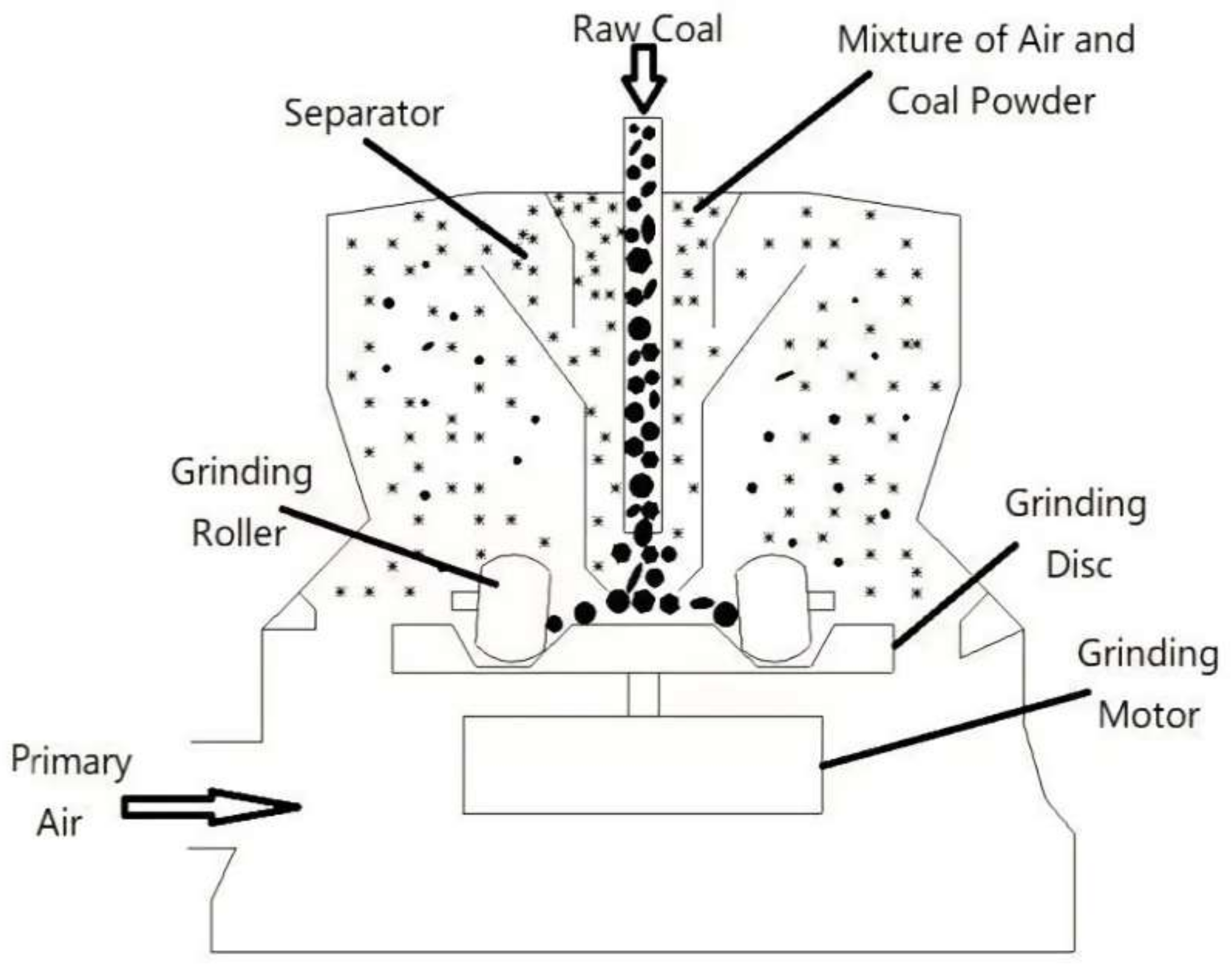
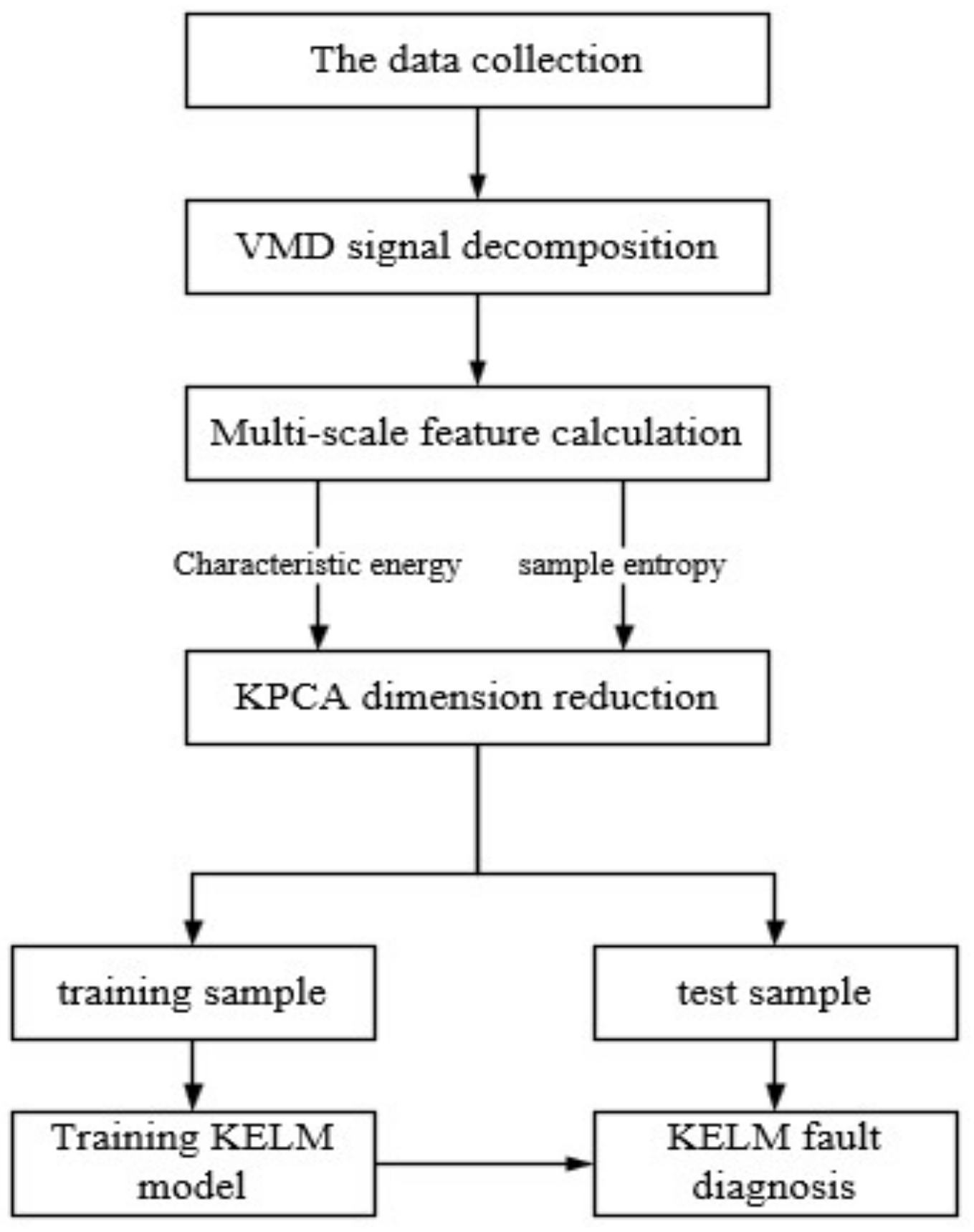
The vibration signals of a medium-speed coal mill under various working conditions are collected, and the abnormal values are processed; then, the bad points are removed to form the vibration signal sequence.

(2)

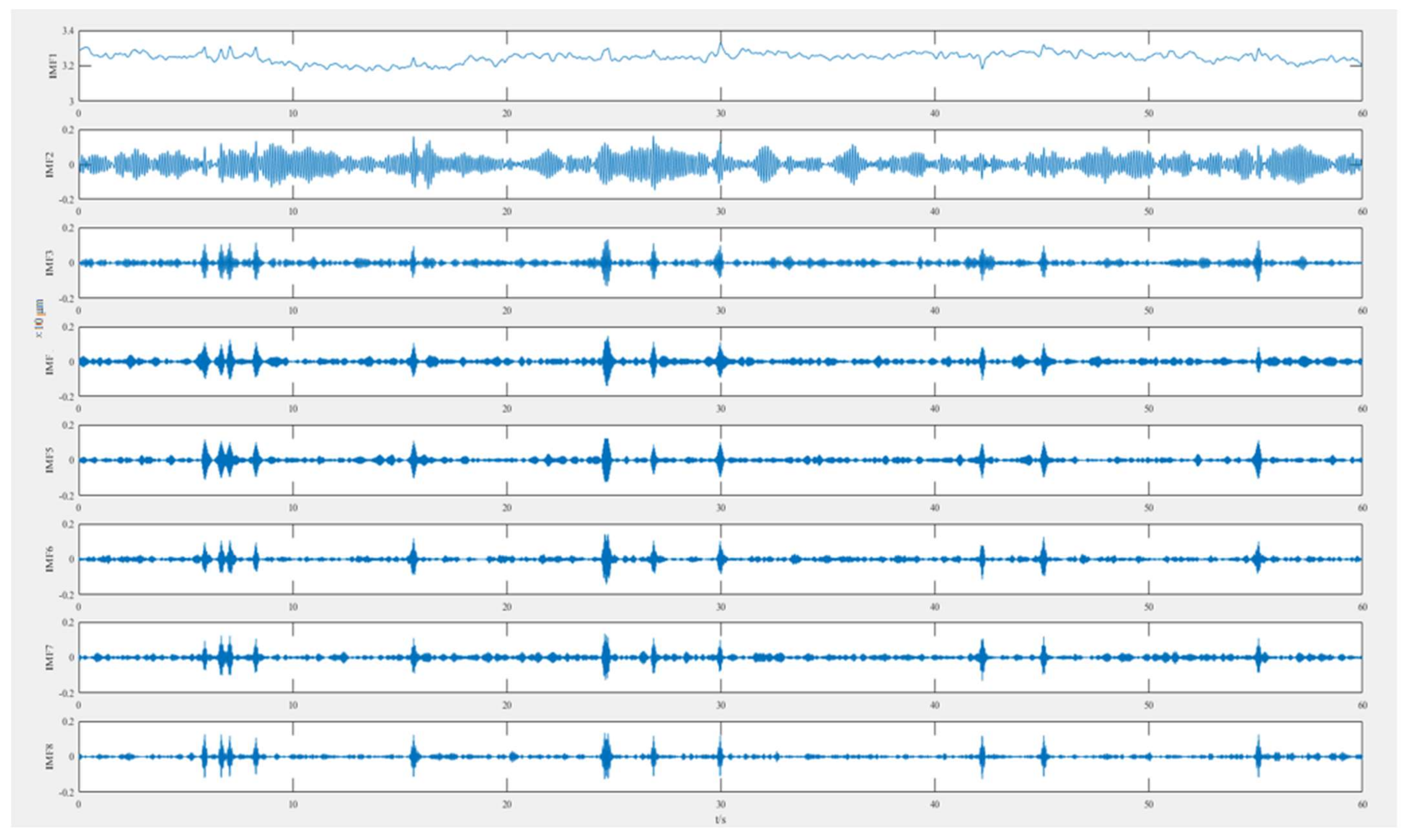
The VMD signal decomposition method described in 2.1.1 (Formulas 1–5) is used to decompose the vibration signal of the coal mill to obtain the distribution change of the intrinsic mode function.

(3)

The feature extraction method described in 2.1.2 is used to calculate the intrinsic mode functions obtained in (2), in which the sample entropy is calculated by Formulas 8–13; the characteristic energy is calculated by Formulas 14–15.

(4)

The kernel principal component analysis is carried out on the feature data set composed of sample entropy and feature energy by Formulas 16–24, and the CPV is used as an index to realize data dimension reduction.

(5)

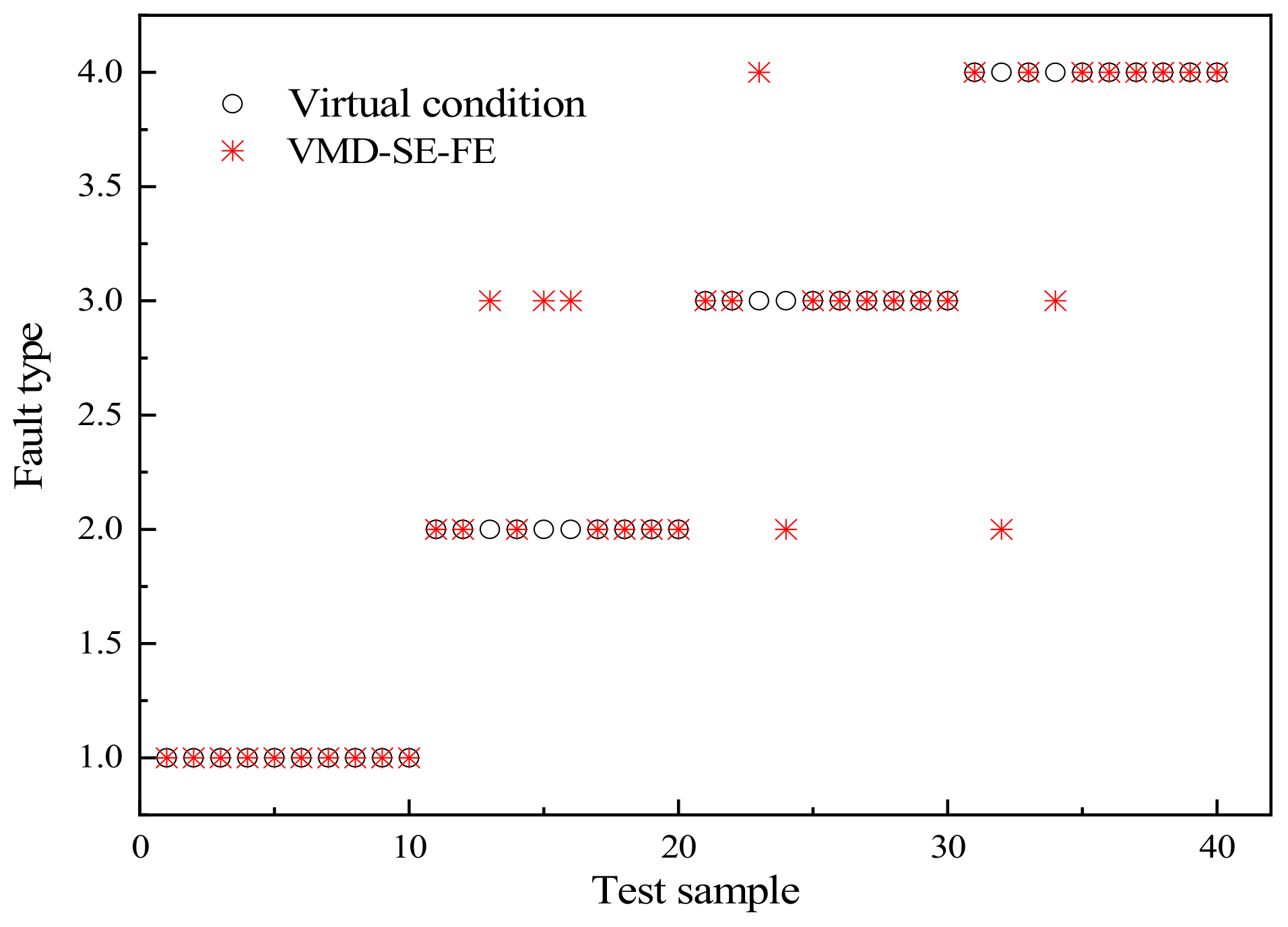
The dimension-reduced fault label data are divided into a training set and a test set. The GA-KELM model described in 2.2 is used to train the training set, and then the test set is used to evaluate the diagnostic accuracy of the model.

The VMD-FE+SE-KPCA-KELM fault diagnosis model was trained by using vibration signals corresponding to the four states of the coal mill, and then the state of the test samples was predicted. The KELM, the VMD-FE-KELM, the VMD-SE-KELM the VMD-FE+SE-KELM and the VMD-FE+SE-PCA-KELM are respectively compared with the VMD-FE+SE-KPCA-KELM fault diagnosis model to verify the model performance. The VMD decomposition diagram of the vibration signal in the insufficient loading pressure state of the coal mill is shown in Figure 3. The distribution of sample entropy proportion after VMD decomposition of vibration signal is shown in

Table 3. The distribution of sample entropy corresponding to the IMF under each fault state.

	IMF1	IMF2	IMF3	IMF4	IMF5	IMF6	IMF7	IMF8
Fault 1	0.0523	0.3394	0.5420	0.5384	0.4853	0.4084	0.2518	0.0500
Fault 1	0.0560	0.2238	0.5133	0.6298	0.5637	0.3849	0.1747	0.0496
Fault 2	0.0880	0.5982	1.3503	1.4385	1.3853	1.2403	0.6876	0.2654
Fault 2	0.0845	0.5889	1.3017	1.4184	1.2870	1.1994	0.7982	0.3461
Fault 3	0.1351	0.7370	1.3986	1.4055	1.3835	1.3403	1.0675	0.4099
Fault 3	0.1061	0.8253	1.2439	1.4709	1.3817	1.2144	0.8679	0.3727

. After VMD decomposition, the sample entropy and feature energy are combined to perform KPCA processing, and the first three terms are taken as state characterization parameters. The obtained distribution is shown in

Table 4. The distribution of state parameters after KPCA in each fault state.

Label	PC1	PC2	PC 3	Label	PC1	PC2	PC3
1	0.687	1.994	−1.998	2	−4.046	−0.433	0.435
1	−0.060	2.237	−1.020	3	−3.383	−1.699	0.464
2	−4.046	−0.433	0.435	3	−3.090	−1.760	0.355

.

It can be seen from Figure 2 that the vibration signal of insufficient loading pressure of the pulverizer increases with the number of decomposition layers of VMD, and the sample entropy and characteristic energy of the vibration signal tend to be stable. After IMF3, the entropy and characteristic energy of vibration signal samples basically do not change.

Table 3 and Table 4 show that after VMD decomposition of vibration signals, sample entropy and feature energy calculation can obtain a certain rule of state characterization, while the kernel principal component analysis of the combination of sample entropy and feature energy can reduce the number of characteristic parameters and reflect the information contained in vibration signals more accurately.

The kernel parameters and regularization coefficients of extreme learning machine have an important influence on model performance. In this paper, the particle swarm optimization (PSO) algorithm is used to optimize the above parameters, and fitness is taken as a reference index. The PSO algorithm is set as a population number. The results of optimizing parameters of the KELM model under the four feature extraction methods are shown in

Table 5. Optimization results of KELM model parameters for different feature extraction.

Model	Regularization Coefficient	Kernel Parameters
VMD-SE	37.43	8.43
VMD-FE	46.26	1.21
VMD-FE-SE	68.52	0.83
FE-SE-PCA	78.16	2.21
FE-SE-KPCA	186.15	3.25

, indicating that the optimal regularization coefficient and kernel function parameters corresponding to each feature extraction prediction model are different. Among them, the optimal regularization coefficient of the VMD-Se+Fe-KPCA model is large, which is 186.1453, while the kernel function is 3.2548.

The distribution of fault diagnosis accuracy and results based on feature extraction is shown in

Table 6. Performance comparison of fault diagnosis models based on nuclear extreme learning machine.

Model	Training Accuracy (%)	Testing Accuracy (%)	Testing Time (s)
KELM	89.2	67.5	9.36
VMD-SE	86.7	70	12.63
VMD-FE	89.2	77.5	13.92
VMD-FE+SE	96.6	82.50	25.27
FE+SE+PCA	95	80	18.49
FE+SE+KPCA	95.8	87.5	16.49

and Figure 4 and Figure 5.

Compared with the single KELM model, the training and testing accuracy of the KELM model based on feature extraction is significantly improved, indicating that the feature extraction of vibration signals is beneficial to the display of positive information in the signal, which can improve the accuracy of the model diagnosis and classification because diagnostic model can obtain the representation state parameters.

The test accuracy of the diagnostic models using sample entropy and feature energy individually are 70% and 80%, respectively, and the sample entropy can further represent the fault features. The feature energy and sample entropy are used together as fault feature parameters, variables that can reflect strong fault characteristics in the model input parameters increases, which can further improve the prediction accuracy of the KELM model. However, due to the increase in the input sample space dimension, the increased test time and time cost will negatively influence the online real-time monitoring of faults. When the feature parameters of sample entropy and feature energy after the kernel principal component analysis are used as the model input, the test accuracy of the model is more optimal than that of the model without kernel principal component analysis, and the time cost of the test is reduced. This reveals that the introduction of the kernel principal component analysis algorithm can realize the dimension reduction of the original sample space and the calculation cost. In addition, it can realize the noise reduction function of the sample, which can enhance the model test accuracy, providing a reference for the real-time state monitoring of coal mill failures.

4. Conclusions

In this paper, a kernel extreme learning machine model based on feature extraction and kernel principal component analysis is proposed for fault diagnosis of coal mill. The experimental data of mill vibration signals under different faults and the performance of several models are compared. The results show that: (1) compared with single feature extraction, multi-feature extraction of fault signal decomposition can significantly enhance fault features and improve model performance; (2) the kernel principal component analysis algorithm not only realizes the dimension reduction of the original sample space, reduces information redundancy and reduces computing cost but also realizes the sample noise reduction function, which is conducive to improving the test accuracy of the feature extraction model, and provides a new idea for the fault diagnosis of coal mill based on feature extraction.

References

1. Hu, Y.; Ping, B.Y.; Zeng, D.L.; Niu, Y.G.; Gao, Y.K.; Zhang, D.M. Research on fault diagnosis of coal mill system based on the simulated typical fault samples. Measurement 2020, 161, 107864. [Google Scholar] [CrossRef]
2. Gao, Y.; Zeng, D.; Liu, J.; Jian, Y. Optimization control of a pulverizing system on the basis of the estimation of the outlet coal powder flow of a coal mill. Control Eng. Pract. 2017, 63, 69–80. [Google Scholar] [CrossRef]
3. Zhu, L.; Liu, S.; Zhang, D.; Qiu, X.; Zhou, W. Coal mill fault diagnosis based on Gaussian process regression. IOP Conf. Ser. Earth Environ. Sci. 2019, 332, 042034. [Google Scholar] [CrossRef]
4. Agrawal, V.; Panigrahi, B.K.; Subbarao, P. Intelligent Decision Support System for Detection and Root Cause Analysis of Faults in Coal Mills. IEEE Trans. Fuzzy Syst. 2017, 25, 934–944. [Google Scholar] [CrossRef]
5. Fan, G.Q.; Rees, N.W. An intelligent expert system (KBOSS) for power plant coal mill supervision and control-ScienceDirect. Control Eng. Pract. 1997, 5, 101–108. [Google Scholar] [CrossRef]
6. Wang, J.; Wei, J.; Shen, G. Condition Monitoring of Power Plant Milling Process Using Intelligent Optimisation and Model Based Techniques. Fault Detect. 2010, 19, 405–423. [Google Scholar]
7. Wang, J.; Wei, J.; Zachariades, P.; Guo, S. On-line condition and safety monitoring of pulverised coal mills using a mode based pattern recognition technique. In Project B85A; The University of Birmingham, BCURA: Birmingham, UK, 2009. [Google Scholar]
8. Guo, S.; Wang, J.; Wei, J.; Zachariades, P. A new model-based approach for power plant Tube-ball mill condition monitoring and fault detection. Energy Convers. Manag. 2014, 80, 10–19. [Google Scholar] [CrossRef] [Green Version]
9. Wei, J.L.; Wang, J.; Wu, Q.H. Development of a Multisegment Coal Mill Model Using an Evolutionary Computation Technique. IEEE Trans. Energy Convers. 2007, 22, 718–727. [Google Scholar] [CrossRef]
10. Su, Z.G.; Wang, P.H.; Yu, X.J.; Lv, Z.Z. Experimental investigation of vibration signal of an industrial tubular ball mill: Monitoring and diagnosing. Miner. Eng. 2008, 21, 699–710. [Google Scholar] [CrossRef]
11. Kisic, E.; Petrovic, V.; Vujnovic, S.; Durovic, Z.; Ivezic, M. Analysis of the condition of coal grinding mills in thermal power plants based on the T multivariate control chart applied on acoustic measurements. Facta Univ.-Ser. Autom. Control Robot. 2012, 11, 141–151. [Google Scholar]
12. Tao, X.U.; Wang, Q. Application of Multiscale Principal Component Analysis Based on Wavelet Packet in Sensor Fault Diagnosis. Proc. Csee 2007, 27, 28. [Google Scholar]
13. Si, D.T. The Fourier Transform and Principles of Quantum Mechanics. Appl. Math. 2018, 9, 347–354. [Google Scholar] [CrossRef] [Green Version]
14. Bagheri, A.; Fatemi, A.A.; Amiri, G.G. Simulation of earthquake records by means of empirical mode decomposition and Hilbert spectral analysis. J. Earthq. Tsunami 2014, 8, 1450002. [Google Scholar] [CrossRef]
15. Dragomiretskiy, K.; Zosso, D. Variational Mode Decomposition. IEEE Trans. Signal Processing 2014, 62, 531–544. [Google Scholar] [CrossRef]
16. Zhu, Q.; Chen, X.; He, Y.; Lin, X.; Gu, X. Energy efficiency analysis for ethylene plant based on PCA-DEA. Ciesc J. 2015, 66, 278–283. [Google Scholar]
17. Bounoua, W.; Bakdi, A. Fault detection and diagnosis of nonlinear dynamical processes through correlation dimension and fractal analysis based dynamic kernel PCA. Chem. Eng. Sci. 2021, 229, 116099. [Google Scholar] [CrossRef]
18. Amin, M.T.; Khan, F.; Ahmed, S.; Imtiaz, S. A data-driven Bayesian network learning method for process fault diagnosis. Process Saf. Environ. Prot. 2021, 150, 110–122. [Google Scholar] [CrossRef]
19. Cao, W.; Wang, X.; Ming, Z.; Gao, J. A review on neural networks with random weights. Neurocomputing 2018, 275, 278–287. [Google Scholar] [CrossRef]
20. Tamilselvan, P.; Wang, P. Failure diagnosis using deep belief learning based health state classification. Reliab. Eng. Syst. Saf. 2013, 115, 124–135. [Google Scholar] [CrossRef]
21. Huang, G.B.; Wang, D.H.; Lan, Y. Extreme Learning Machines: A Survey. Int. J. Mach. Learn. Cybern. 2011, 2, 107–122. [Google Scholar] [CrossRef]
22. Huang, G.B.; Zhu, Q.Y.; Siew, C.K. Extreme learning machine: Theory and applications. Neurocomputing 2006, 70, 489–501. [Google Scholar] [CrossRef]
23. Goel, T.; Murugan, R. Classifier for Face Recognition Based on Deep Convolutional-Optimized Kernel Extreme Learning Machine. Comput. Electr. Eng. 2020, 85, 159–164. [Google Scholar] [CrossRef]
24. Khoshnami, A.; Sadeghkhani, I. Sample entropy-based fault detection for photovoltaic arrays. IET Renew. Power Gener. 2018, 12, 1966–1976. [Google Scholar] [CrossRef]
25. Pahon, E.; Steiner, N.Y.; Jemei, S.; Hissel, D.; Pera, M.C.; Wang, K.; Mocoteguy, P. Solid oxide fuel cell fault diagnosis and ageing estimation based on wavelet transform approach. Int. J. Hydrog. Energy 2016, 41, 13678–13687. [Google Scholar] [CrossRef]
26. Huang, G.; Huang, G.B.; Song, S.; You, K. Trends in extreme learning machines: A review. Neural Netw. 2015, 61, 32–48. [Google Scholar] [CrossRef]
27. Wen, H.; Fan, H.; Xie, W.; Pei, J. Hybrid Structure-Adaptive RBF-ELM Network Classifier. IEEE Access 2017, 5, 16539–16554. [Google Scholar] [CrossRef]
28. Ahmadi, M.H.; Ahmadi, M.A.; Nazari, M.A.; Mahian, O.; Ghasempour, R. A proposed model to predict thermal conductivity ratio of Al2O3/EG nanofluid by applying least squares support vector machine (LSSVM) and genetic algorithm as a connectionist approach. J. Therm. Anal. Calorim. 2018, 135, 271–281. [Google Scholar] [CrossRef]
29. Muhammad, A.R.; Yuan, X.; Ozgur, K.; Muhammad, A.; Asif, M. Stream Flow Forecasting of Poorly Gauged Mountainous Watershed by Least Square Support Vector Machine, Fuzzy Genetic Algorithm and M5 Model Tree Using Climatic Data from Nearby Station. Water Resour. Manag. 2018, 32, 4469–4486. [Google Scholar]
30. Wan, J.; Li, S. Modeling and application of industrial process fault detection based on pruning vine copula. Chemom. Intell. Lab. Syst. 2019, 184, 1–13. [Google Scholar] [CrossRef]
31. Ren, X.; Zhu, K.; Cai, T.; Li, S. Fault Detection and Diagnosis for Nonlinear and Non-Gaussian Processes Based on Copula Subspace Division. Ind. Eng. Chem. Res. 2017, 56, 11545–11564. [Google Scholar] [CrossRef]
Figure 1. Schematic diagram of the working principle of MPS medium speed coal mill [1].
Energies 15 05385 g001
Figure 2. VMD-FE+SE-KPCA-KELM modeling flow chart.
Energies 15 05385 g002
Figure 3. VMD decomposition diagram of the vibration signal in the different loading state.
Energies 15 05385 g003
Figure 4. Prediction results of kernel extreme learning machine model based on VMD-FE+SE.
Energies 15 05385 g004
Figure 5. Prediction results of kernel extreme learning machine model based on VMD-FE+SE-KPCA.
Energies 15 05385 g005