
Hybrid Game Optimization of Microgrid Cluster (MC) Based on Service Provider (SP) and Tiered Carbon Price


1
School of Mechatronic Engineering and Automation, Shanghai University, Shanghai 200444, China
2
Jiangsu Provincial Research and Development Center of Energy Internet and Large Data Integration Application Engineering Technology, Changzhou Vocational Institute of Engineering, Changzhou 213164, China
3
School of Electrical Engineering, Southeast University, Nanjing 210096, China
*
Author to whom correspondence should be addressed.
Energies 2022, 15(14), 5291; https://doi.org/10.3390/en15145291
Submission received: 3 June 2022
/
Revised: 1 July 2022
/
Accepted: 12 July 2022
/
Published: 21 July 2022
Abstract
:Carbon trading is a market-based mechanism towards low-carbon electric power systems. A hy-brid game optimization model is established for deriving the optimal trading price between mi-crogrids (MGs) as well as providing the optimal pricing scheme for trading between the microgrid cluster(MC) and the upper-layer service provider (SP). At first, we propose a robust optimization model of microgrid clusters from the perspective of risk aversion, in which the uncertainty of wind and photovoltaic (PV) output is modeled with resort to the information gap decision theo-ry(IGDT). Finally, based on the Nash bargaining theory, the electric power transaction payment model between MGs is established, and the alternating direction multiplier method (ADMM) is used to solve it, thus effectively protecting the privacy of each subject. It shows that the proposed strategy is able to quantify the uncertainty of wind and PV factors on dispatching operations. At the same time, carbon emission could be effectively reduced by following the tiered carbon price scheme.
1. Introduction
Many carbon emission trading schemes have been proposed and implemented worldwide in recent decades to slow or stop human-caused global warming [1]. The European union emissions trading system was initiated in 2005 by the EU and is still considered to be the largest single market for emission allowance trading [2]. In pursuance of the commitment to realize a carbon emissions peak in 2030 and achieve carbon neutrality in 2060, China launched the world’s largest carbon trading market in Shanghai on 16 July 2021 [3,4].
The operation of the power system naturally brings about, for example, combustion of fossil fuel [5,6]. To reduce the volume of carbon emissions in the operation of the power system, smart grid technologies had been significantly introduced in the last two decades, as they possess the capability of integrating multiple low-carbon renewable energy sources, such as photovoltaic (PV) and wind [7]. In recent years, the concepts of microgrid (MG) and microgrid cluster (MC) have become more and more popular in the smart grid community [8]. MG is a small-scale electrical power grid that consists of microgeneration units, storage units, and controllable loads. Microgrid clusters refer to multiple interconnected microgrids that facilitate energy exchange among the participating prosumers, producers, and customers. For the sake of carbon reduction in a smart grid, a promising way is to formulate a carbon emission trading incorporated energy management system within the architecture of MCs [9,10].
The trading price plays a decisive role in the designing of trading systems. Regarding the energy transaction of MCs, it is a challenging task to generate a fair price that balances the demands of prosumers, producers, and customers, as the demands are often competitive and conflictive [11]. In the related literature, game theory was extensively employed to seek the promising transaction modes in a smart grid society. In [12,13], the Stackelberg game model is utilized to generate the transaction price between MC and MG, in which the relationship of MC and MG is viewed as leader and follower. In [14,15], cooperative game models are created to reveal the cooperative and competitive behaviors of MCs. Furthermore, with the aid of Nash bargaining theory, cooperative game models can also be used simultaneously for multi-objective optimization, such as maximizing both the annual profit and the energy index of reliability [16,17]. It is pointed out that the Nash bargaining technique leads to a faster convergence than the heuristic algorithms that are equipped with remedies such as greedy or linear relaxation [18]. To realize the goal of carbon emission reduction, not only interplay of MCs, but also the transaction between MCs and the other market players of the main grid should be take into consideration. This makes it a complex optimization problem with many more decision variables; at the same time, it is difficult to produce a promising carbon trading price mechanism by applying existing game theory-based methods directly.
The high-penetration rate of renewable energy such as wind and PV in MCs provide a great potential for carbon emission reduction. However, modeling of MCs becomes technically challenging due to the inherent climate-dependent uncertainty of wind and PV [19,20]. Generally speaking, commonly used mathematical tools to cope with uncertainties include but are not limited to stochastic optimization [21,22], robust optimization [23,24], interval optimization [25,26], and distributionally robust optimization [27,28], to name a few. A scenario generation scheme is used to capture the strong randomness and interdependence between wind speeds by utilizing historical wind data, which leads to reliable Microgrid scheduling results by resorting to stochastic programming [29]. In [30], the wind speed uncertainty is modeled as a colored noise via a second-order autoregressive model; on that basis, a stochastic program is solved to increase the expected value of the profit distribution and keep the risk of profit variability controllable. In [31,32], an interval optimization method was facilitated to generate robust system dispatchers for combating fluctuation of wind power and photovoltaic over pre-specified intervals. In addition to a priori knowledge of the uncertainties, the tractability and computational efficiency of the recast optimization problems also play an important role in the development of techniques and tools for dealing with the uncertainties. Information gap decision theory (IGDT) is a powerful tool converting stochastic uncertainty into a deterministic setting. In [33,34], IGDT was introduced to describe the uncertainty of wind and PV, and a bi-layer stochastic optimization model was established to solve the day-ahead dispatching of MGs.
This paper aims to solve the carbon allowance allocation and the uncertainty problem based on renewable energy (RE), which develops a hybrid game optimization of carbon emissions considering a tiered price for SP with MC. In this paper, the MC dispatch model of carbon capture system (CCS) is given, and the risk aversion strategy is used to deal with the uncertainty of wind and PV. Furthermore, it shows that the carbon emission of MC is influenced by guiding the carbon price. Finally, the effectiveness of the proposed method in the collaborative optimization of MC is verified, and the uncertainty of wind and PV and tiered price are analyzed to verify the feasibility of using the hybrid game optimization in the case study.
Briefly, the contributions of the paper can be summarized as follows:
- The MC system considering the tiered carbon price is proposed in this paper, which combines with the service provider (SP) to provide the electricity purchase/sale price for the MC to access the utility grid.
- The risk-avoidance strategy is adopted to consider the uncertainty of wind and PV, and the information gap decision theory (IGDT) is used to solve the robust dispatch model of its uncertainty.
- A new hybrid game model is adopted, which uses the stackelberg game to deal with the relationship between SP and MC and uses Nash equilibrium theory to solve the payment interests among MGs.
2. System Modelling
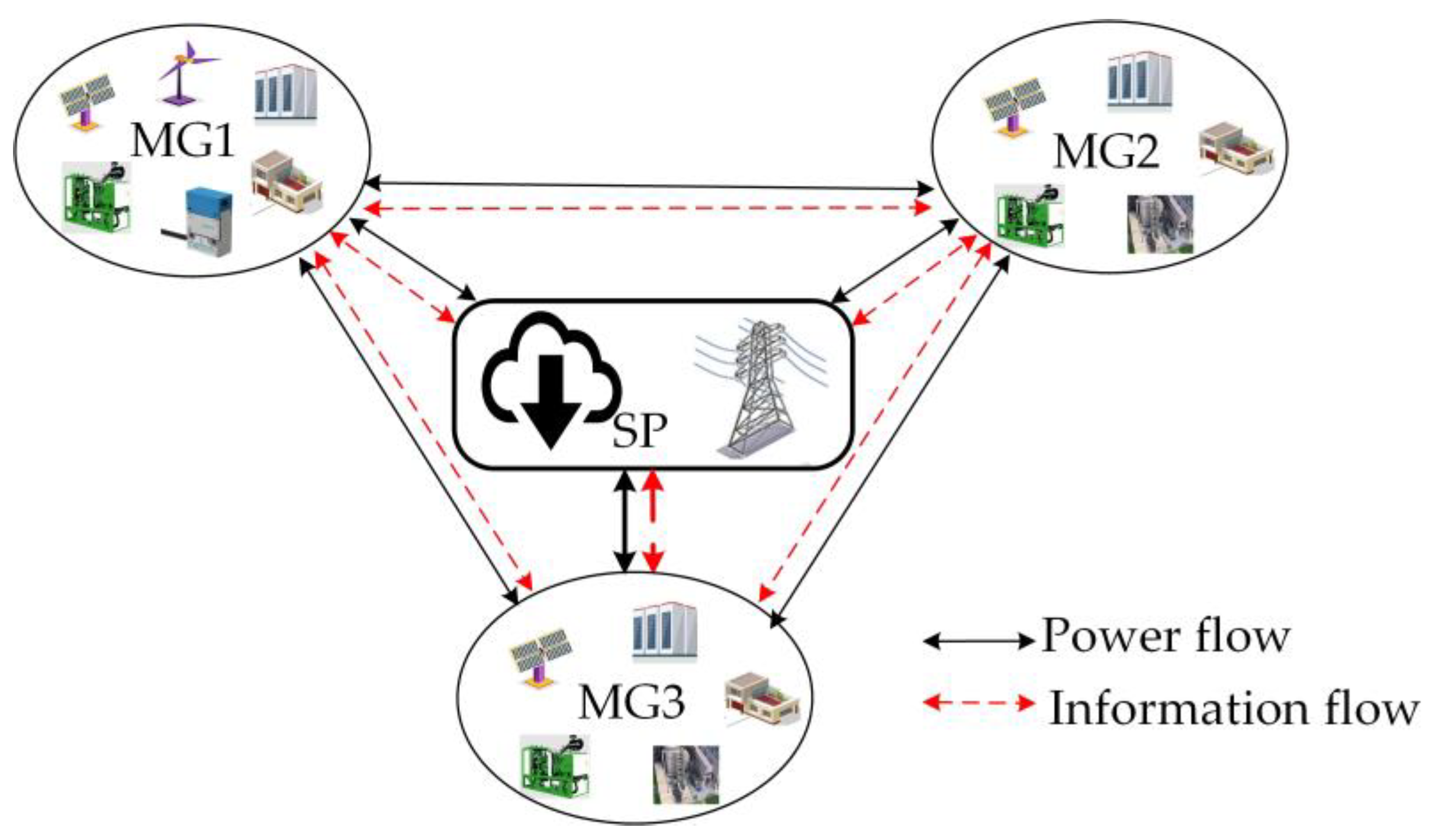
In this study, in order to evaluate the proposed method, service providers are used to dispatch the MC composed of three MGs, as shown in Figure 1. In addition, MG1 contains different units from MG2 and MG3. MG1 contains RE, combined heat and power generation (CHP), ground source heat pump (GSHP), and CCS, etc., whereas MG2 and MG3 contain GT, GB, and CCS, etc.
The following sections contain the detailed modelling of the entities.
2.1. System Structure
Each MG has an operator that manages its own unit and trading power simultaneously with other MGs and the SP. A discrete time model with a 24 h horizon is considered. We assume that the time interval is 1 h, so there are 24 decisions in the dispatching cycle.
2.2. MG Modelling
In this study, a carbon trading MG is proposed, and the objective function and related constraint operating in the inter trading mode are as follows:
- Objective function of each MG:
Objective function of the ith MG includes four terms referred to as the cost of trading power from the utility grid, cost of natural gas combustion, maintenance cost of discharge/charge power with ES and HS, and cost of carbon trading. The tiered carbon emission price in the interval is shown in Figure 2. Note that the carbon price in the 0th and 1st interval is p0, whereas the actual carbon emission is less than the quota quality. The carbon price is related to both the vth interval and the increment σ in the interval 1 ≤ v ≤ V, and the carbon quota is less than the actual emission. When the carbon emission exceeds the Vth interval, the carbon price is only related to the increment σ. There is the index for time, which is used for hourly dispatch. The constraints, which are related to each unit of the MG, are as follows:
- CHP operating constraints:
Equation (2) is the operation mode of ordering electric by heat. Equation (3) refers to the ramp rate limitation. Constraints (4) and (5) express the allowable electric and heat power of CHP. Calculation of the natural gas volume required for electric power generated by CHP uses Equation (6).
- GB and GT constraints:
Constraint (7) is the coupling relation between electric and heat. Constraints (8) and (9) indicate the allowable electric power of GB and GT. Constraints (10) and (11) stand for electric power generated by GB and GT natural gas. Constraint (12) illustrates the total volume of natural gas between GB and GT.
- ES and HS constraints:
Constraints (13) and (14), (18) and (19) indicate the charging and discharging power limits for the ES and HS. Equations (15) and (20) are the constraints for avoiding simultaneous charging and discharging. The constraints expressing the state of charge of the ES and HS are shown in Equations (17) and (22), and constraints (16) and (21) indicate the permissible limits for the capacity of ES and HS.
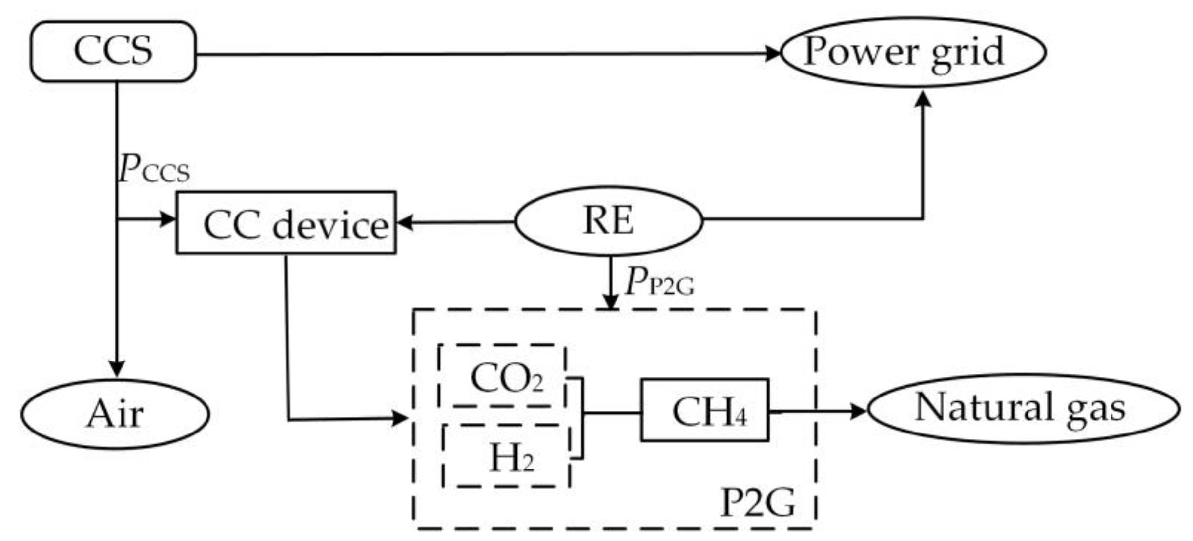
- Cooperative operation of P2G-CCS constraints:
CCS and P2G are coupled to form a joint operation system, as shown in Figure 3. Carbon captured in CCS is used as raw material to supply P2G and synthesize CH4, which can effectively reduce the operation cost. The cooperative operation constraints can be written as follows:
where PP2G and PCCS are electric power consumed of P2G and CCS, respectively; QCC is the CO2 quality required for P2G operation; ηP2G and LP2G are electric to gas efficiency of P2G and calorific value of natural gas, respectively; αCC is the CO2 quality consumed per unit of P2G; and KCC, KGC, and Kbuy are carbon emission intensity of CCS, GT/CHP, and electric power purchased, respectively.
Constraints (23)–(25) indicate the calculable relation of carbon emission and capture. Constraints (26) and (27) designate the limitations for consumption of electrical power of P2G and CCS. Equations (28) and (29) are used to calculate the total carbon emission of CHP after carbon capture.
Compared with the unified carbon price, the tiered carbon price is more suitable for the small carbon emission region and can reduce the carbon emission operating cost, for which the tiered carbon emission model is adopted [35]. The limits of carbon emission in each interval are shown in Equation (30). In particular, carbon emission trading in the 0th interval is 0. Constraint (31) refers to the balance of quota carbon trading within the whole interval.
- GSHP constraints:
The GSHP modelling for steady state in heat exchange can be derived from Equations (32) and (33) as follows.
- RE constraints:
- Exchange power among MGs and with SP constraints:
Equations (35) and (36) are the constraints for exchange power among MGs. Constraint (35) ensures that the exchange power is equal between MGi and MGj, and constraint (36) shows the limitations for the exchange power among MGs. Constraints (37) and (38) stand for the constraints for exchange power between MGi and SP; α is a Boolean variable.
2.3. Service Provider of MG
As the intermediary between MGs and the upper grid, the service provider needs to set the electrical trading price with MGs. The trading of electrical power at any time is to be done in an optimal way from economical and technical perspectives and shall be realized according to the object function of the service provider.
- Objective function of service provider:
Equation (39) represents the benefit maximization of the SP, which takes the benefits of all electrical power benefit minus purchase cost in a period T.
- Transaction price between MGs and SP constraints:
Equations (40) and (41) show the limitations for selling/buying prices. Constraints (42) and (43) are given by the SP to limit the average price of buying/selling electrical power in a period T.
3. Solution Procedure
3.1. The Uncertainty of Wind and PV
Due to the stochastic output power of PV and wind, their power generation depends on the environmental conditions with uncertainty. IGDT is used to establish the uncertainty dispatching model for environmental uncertainty (44):
where αW/αPV is the uncertain radius of wind/PV output; and / is the predicted power out of wind/PV.
Equation (45) shows the comprehensive uncertainty radius of PV and wind. βPV and βW can be determined by using the judgment matrix method according to the demand of PV and wind uncertainty.
The risk avoidance strategy is to seek the maximum uncertainty radius of the uncertain quantity under the condition that the optimization target is within an acceptable range. The larger the uncertainty radius is, the less sensitive the scheme is to the fluctuation of the uncertain quantity, the better the robustness of the model, and the stronger the ability of the system to avoid risks.
Equation (46) refers to the maximum radius of uncertainty; κ is the robustness level factor, and the greater its value, the greater the degree of risk avoidance and the stronger the robustness of the dispatching scheme. It can be seen that the above IGDT robust dispatch model belongs to a two-layer optimization model. The lower layer represents that when the PV and wind output fluctuates in the uncertain set, the operating cost of the system cannot exceed the expected cost value. In order to improve the solving efficiency, Equation (46) is simplified into a single-layer optimization model, as shown in Equation (47).
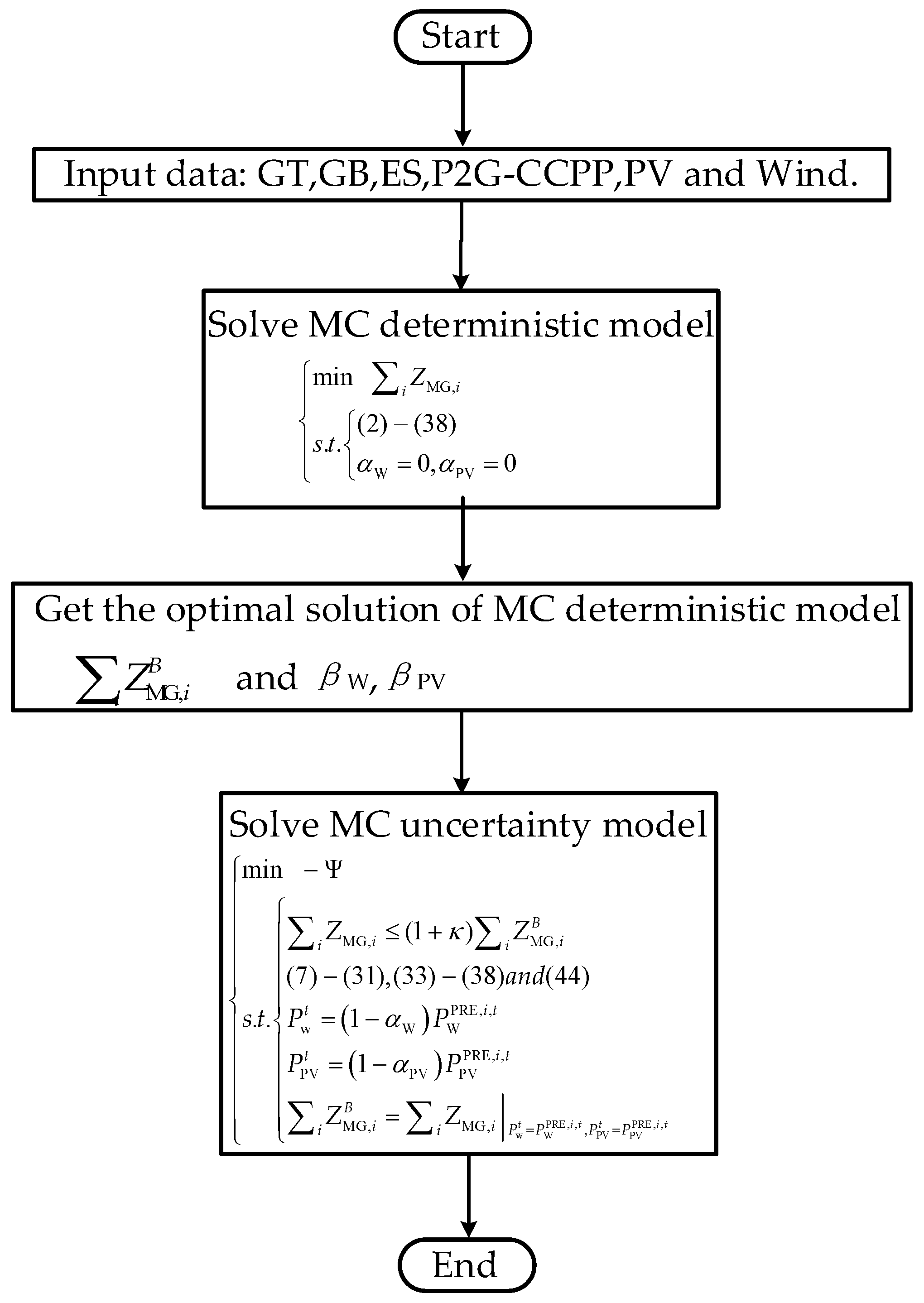
The joint IGDT dispatching strategy of MC considering the uncertainty of PV and wind is shown in Figure 4. First, the MC dispatch model with PV and wind certainty was constructed, and the base operating cost was solved. Next, IGDT is applied to model the uncertainty of PV and wind, and the MC joint robust dispatch model is established and solved according to the risk avoidance strategy.
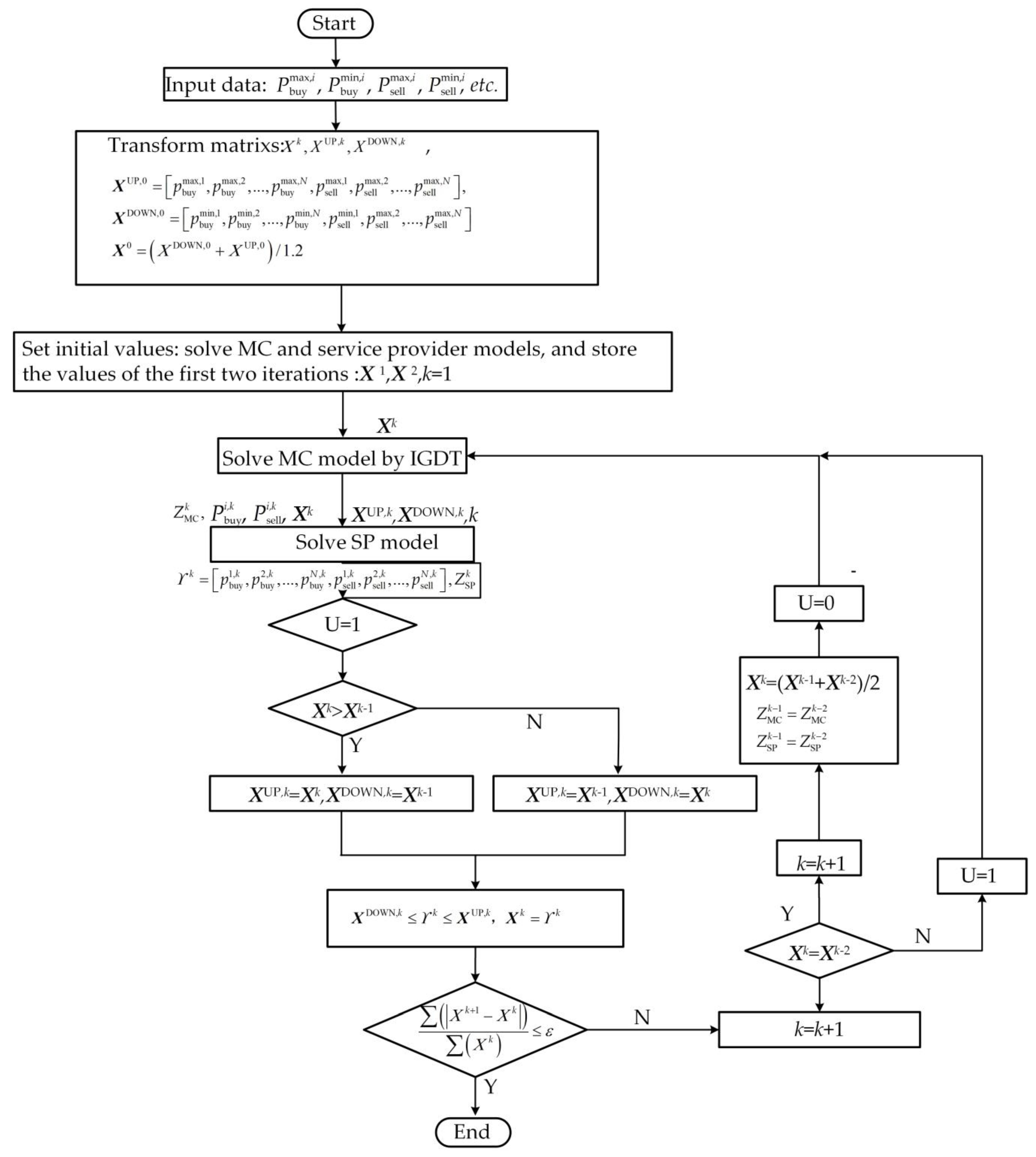
3.2. The Bisection Method for MC with Service Provider
Because the stackelberg game means that the participants are in different positions, the leader can occupy the first opportunity or favorable position in the game, so that the follower can make decisions. SP (leaders) and MC (followers) are considered as two types of interested subjects in this paper. SP order buy/sell electricity prices with the goal of maximizing their profits. Each MG receives the decision from service providers and adjusts its own operation strategies.
For the MC considering the service provider, the higher the selling price, the less electricity the MG purchased. The relationship between the two is monotonically decreasing, so the bisection method is adopted to solve it. Considering the restriction of purchase/sale price, the SP sets the central point (48) in an interval and substitutes it into the IGDT problem.
where X is a set of buying and selling prices between SP and MGs; and k is the iteration.
Similarly, the upper bound or the lower bound is updated by [min (Xk, Xk−1), max (Xk, Xk−1)]. When the algorithm satisfies Equation (49), it converges.
Finally, the dispatching result of IGDT is compared with the objective function, so as to take the buying/selling price interval in half. The specific solution algorithm is shown in Appendix A.
3.3. Nash Solves for Allocating Benefits among MGs
The product of the difference between the maximum benefit obtained by each player in the game and the benefit when the negotiation breaks down (i.e., the lowest benefit) is the Nash negotiation. At this time, the stackelberg equilibrium solution is the optimal solution, and it can also ensure that the interests of all participants are balanced [36]. In this paper, the cooperative game model of MC is given as
where UMG is the profit from MG.
MGs with different interests need to maintain independence and rationality when conducting electricity trading. Using a Nash distributed solution can effectively ensure their own the overall profits; (*) is the breaking point of negotiations.
Taking the logarithm of model (50) and transforming the product problem into a summation problem, the objective function can be transformed into:
For the convenience of solving, the optimal solutions (, ) in model (47) is substituted into Equation (51):
The objective function of model (53) is the natural logarithm, which is a monotonically increasing convex optimization problem. ADMM is used to solve the electricity trading price of MC, so as to ensure the maximum benefit. Therefore, the auxiliary variables and are introduced to decouple the electricity price of MC.
Considering the consistency constraint (54), the augmented Lagrange function (55) is established.
The distributed solution steps of the Nash bargaining game are as follows:
Step1: Initialization parameters: = 0, = = 0, = 10, ε = 0.001, k = 0;
Step2: Each MG calculates its own trading price strategy locally, and only the updated price is exchanged among MGs. In each iteration, the following steps need to be performed:
MGi updates its decision
MGj receives the updated decision , to update its decisions
Step3: Update Lagrange multiplier ;
Step4: k = k + 1;
Step5: Judge convergence;
The iteration terminates if Equation (59) is satisfied. Otherwise, it will go back to Step2 to recalculate until convergence or the set maximum number of iterations is reached.
4. Case Study
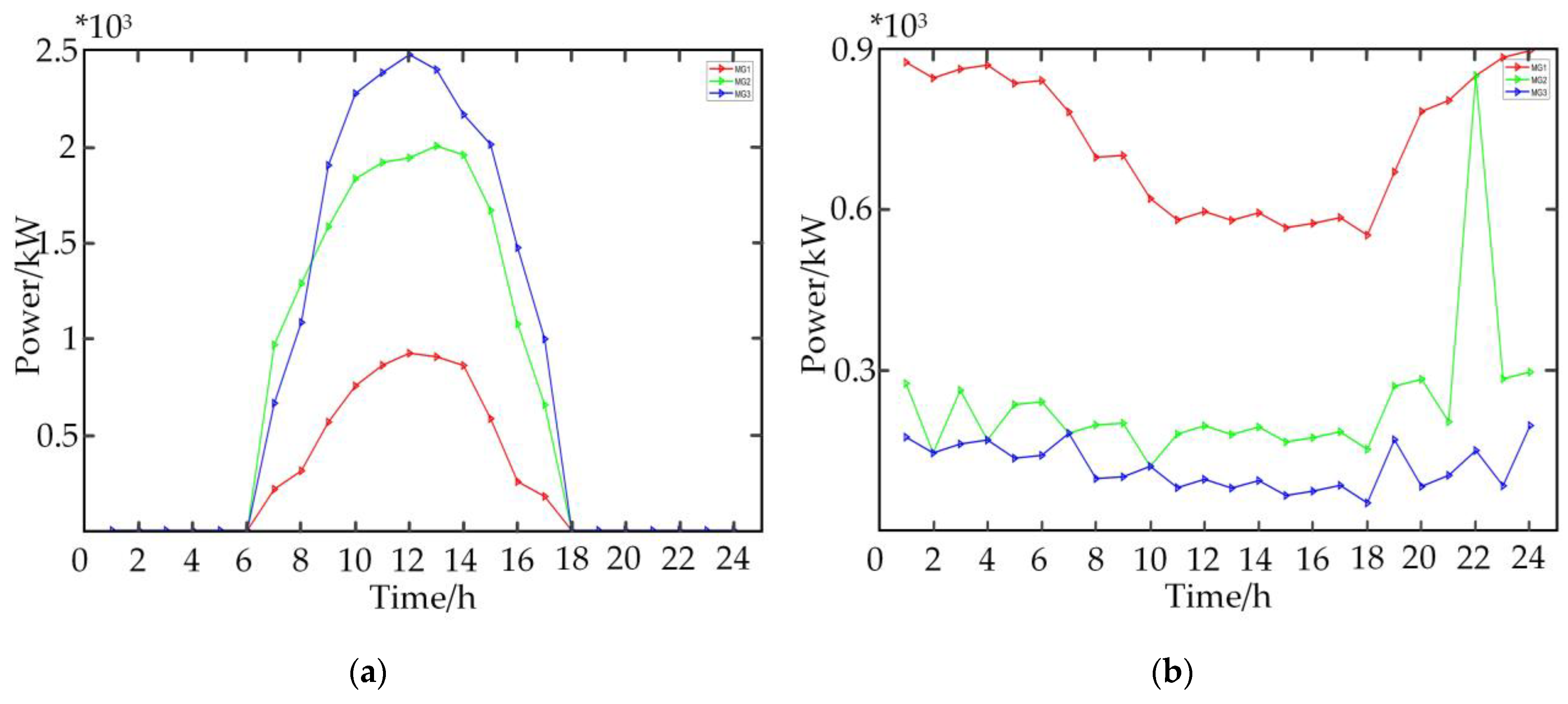
In this section, simulations in a test system are done to demonstrate the changes of the MC optimum energy management using the proposed hybrid game model. The system architecture of the calculation example is shown in Figure 1, and the specific dispatching model of each MG is shown in Appendix B. For the specific parameters of each unit of MGs1–3, refer to Appendices Table A1 and Table A2. The power of RE in MC is shown in Figure 5. The Solver CPLEX in the MATLA2020a environment is employed to perform the energy management.
4.1. Day-Ahead Dispatching Analysis
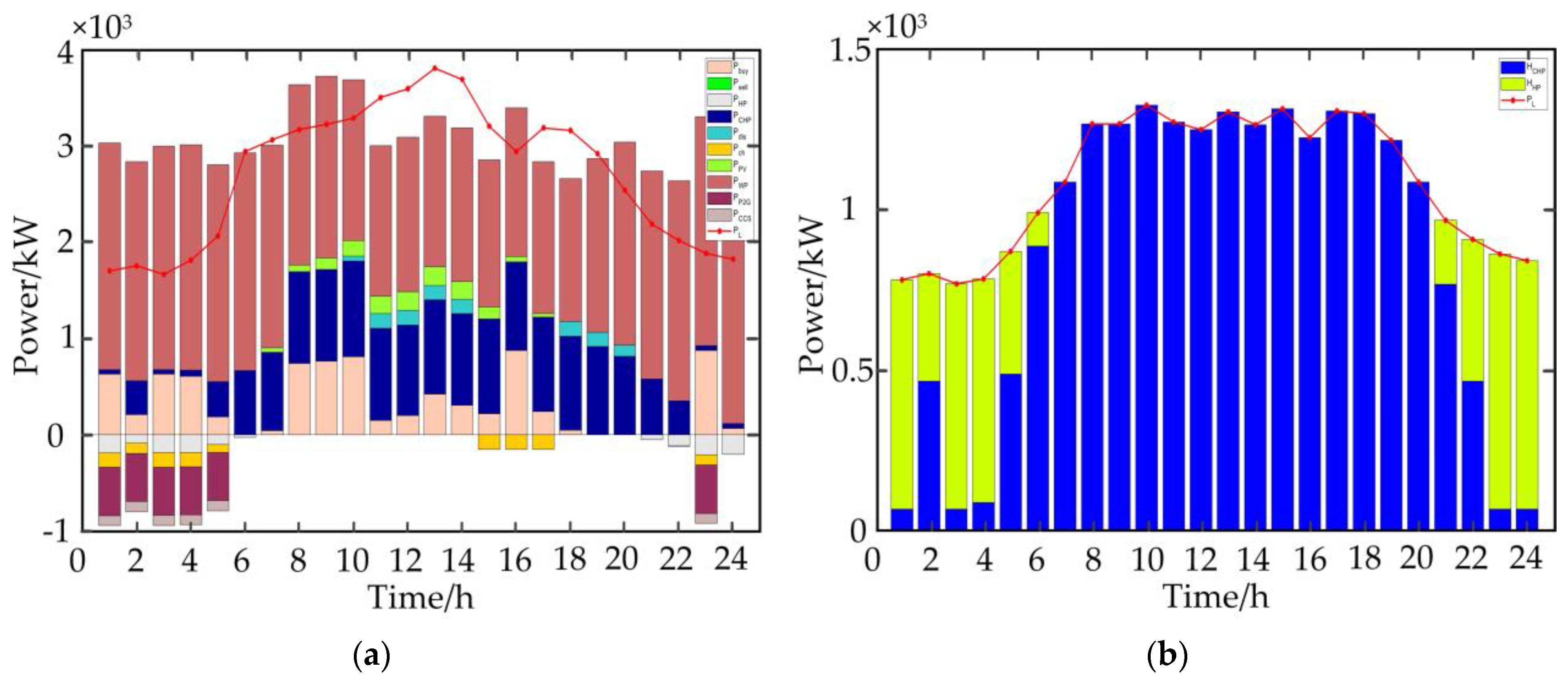
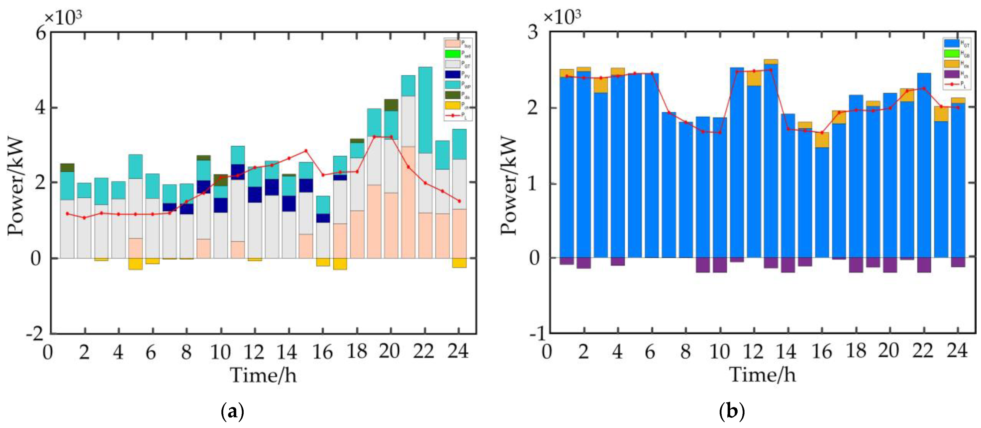
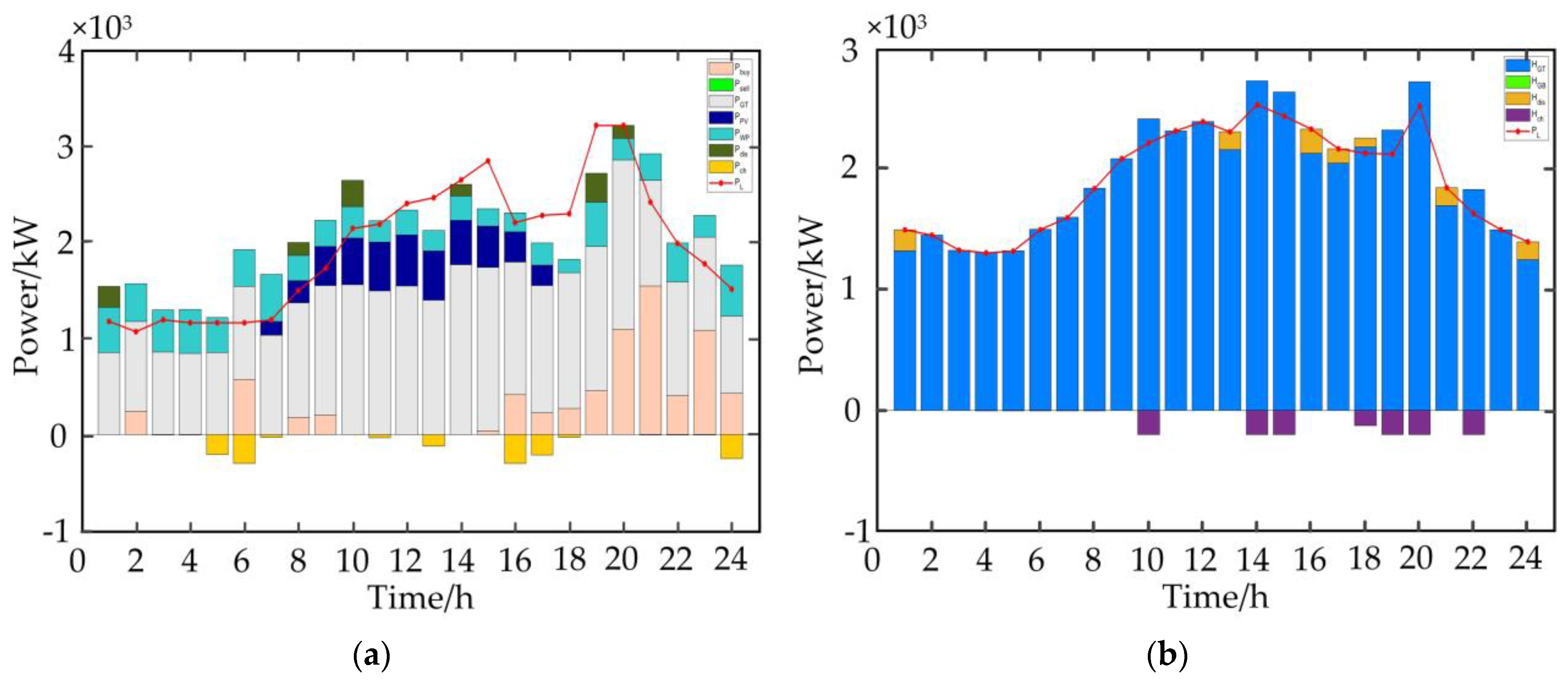
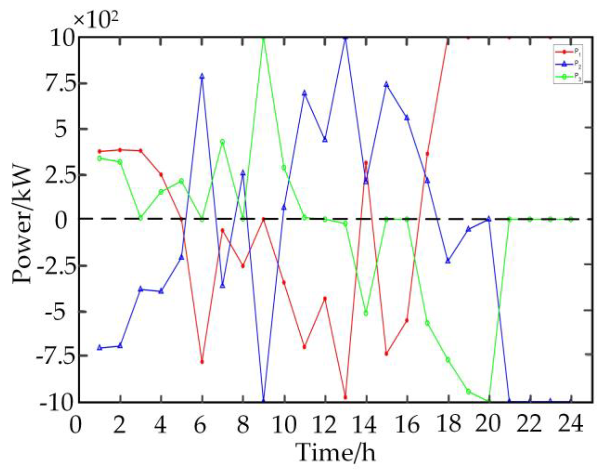
Figure 6, Figure 7 and Figure 8 illustrate the dispatching results of the MC, and the electrical power trading among MGs is depicted in Figure 9, considering two dispatch methods of MC: (1) MG1 adopts deterministic dispatch; (2) the uncertain dispatch is used in MGs2–3. Figure 10 shows electrical power trading among MGs and between the MC and SP, respectively.
As seen from Figure 6a, the electrical load level is relatively low at 1:00–5:00 and 17:00–24:00, and the wind power of MG1 is sufficient to sell electrical power to other MGs. The electrical load reaches the peak from 6:00–16:00; the CHP works at full power. MG1 is buying electrical power from SP and other MGs at the same time. As for the heat load in Figure 6b, the electrical power generated by CHP is relatively low during 1:00–4:00, so the heat power is also too low to meet the heat load demand. At the same time, the heat generated by the HP is sufficient to meet its own heat load demand. Due to working at full power for CHP at 8:00–22:00, the heat power production is sufficient for the heat load.
The low power output of RE in MG2 needs to rely on GT and other MGs to provide electrical power. It can be seen from Figure 7a that the electrical load is relatively low; however, the heat load demand is large, resulting in a relatively high power production of GT, and the surplus electrical power is sold to other MGs. The GT provides a considerable amount of thermal power to meet the load in a day cycle in Figure 7b, and the HS mainly meets the thermal power balance characteristics in the whole system.
In Figure 8a, from 11:00–18:00, the GT of MG3 has insufficient power generation and needs to purchase electric power from MG1. However, at 16:00–20:00, MG3 sells electric power from MG1 and MG2, as seen in Figure 9. In Figure 8b, at 10:00, 14:00–15:00, and 18:00–20:00, the heat power generated by the GT not only meets the human load demand but also charges heat power to the HS.
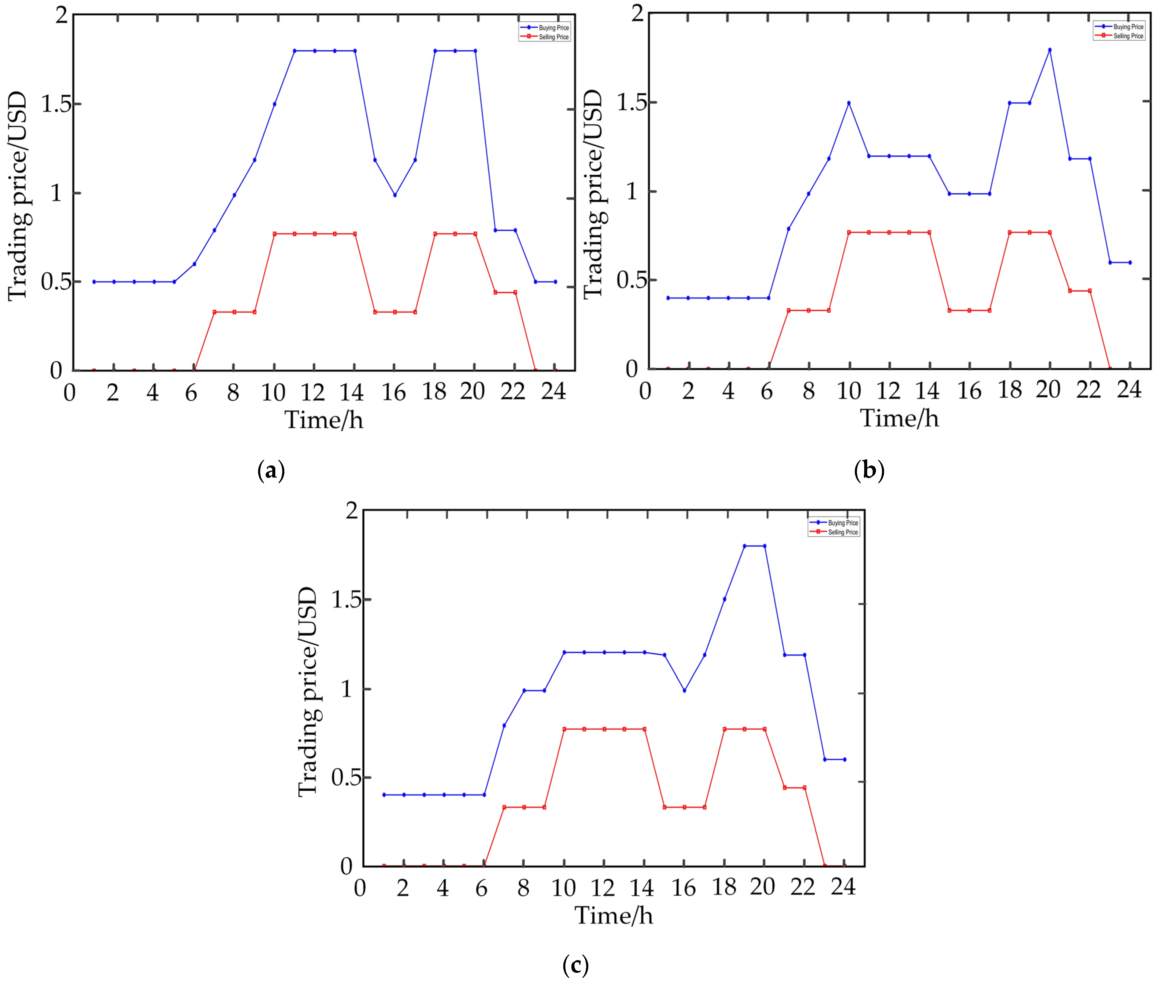
Under the bisection algorithm, the SP also give the selling/buying price of the electrical power transaction to each MG in Figure 10. Taking MG3 as an example, MG3 purchases less electrical power from the utility grid from 1:00–16:00, and the purchase electrical price is also relatively low at this time, as shown in Figure 10c. However, the electrical load of MG3 is in a peak state from 17:00–22:00, and its own unit cannot meet the electrical load demand and needs to purchase power from the utility grid, and the purchase price also rises. The electrical price reaches the limits at 20:00 especially. This means that the purchase electrical price varies with purchased electrical power.
In order to verify the accuracy and speed of the bisection algorithm, compared with the golden cut algorithm, the operating cost of the bisection algorithm is (4.8%, 3.6%, 2.7%) lower than that of the golden cut algorithm in Table 1. As described below, the bisection algorithm converges after eight iterations, whereas the golden cut algorithm requires eleven convergences, showing its capability in terms of computational speed and scalability.
4.2. Analysis of IGDT Dispatching Strategy Considering the Uncertainty of Wind and PV
In order to quantify the influence of each uncertainty factor on the strategy, it is assumed that the robust level factor κ = 0.1 selects different weight coefficients to perform the calculation results of the IGDT robust dispatch model, respectively, as shown in Table 2.
As can be seen from the table, due to the different sensitivities of the system to the fluctuations of various uncertain factors, different weight coefficients will affect the solution results of single uncertain factors. However, it has little influence on the solution result of the whole system. The dispatch decision maker can set each weight coefficient according to the actual situation and historical experience of the system.
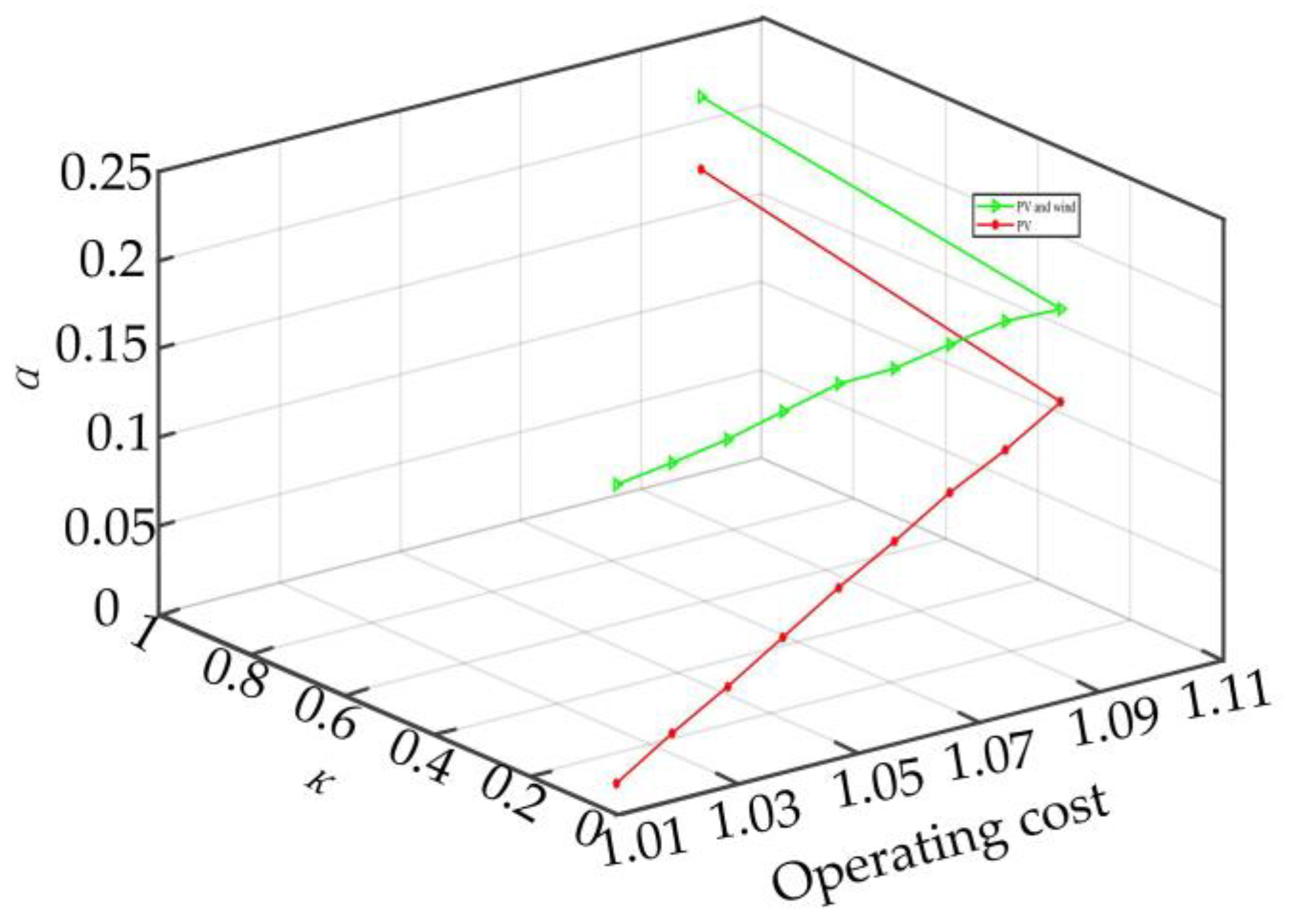
In the risk avoidance model, the robust level factor κ is set to vary from 0 to 0.1, alongside the considered uncertain parameters in two cases studies: (1) PV and wind, and (2) PV.
With the increased operation cost for the MC, α is also increasing from the perspective of overall dispatch in Figure 11. Note that α and operation cost are normalized. Considering more uncertain factors, the effect of risk avoidance is more obvious at this time.
4.3. Environmental Analysis of Tiered Carbon Price
The unified carbon price in all intervals is considered to be 2.9 USD/t in this paper, the tiered price given is 2.5 USD/t in sector 0, and the other intervals are calculated according to model (1). The tiered price results are shown in Table A3.
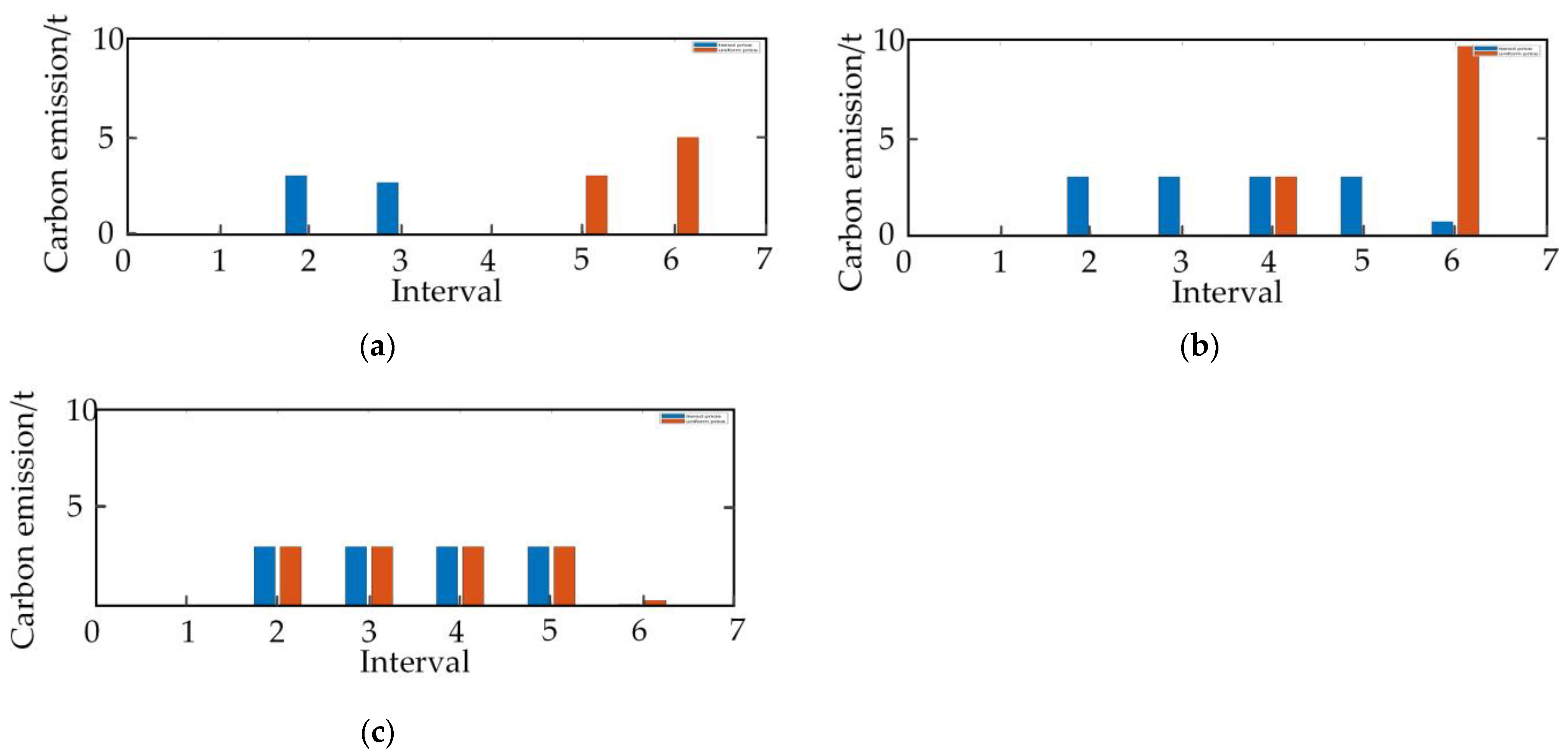
The interval price will increase with the increase of carbon emissions, but the uniform price will not. As can be seen from Figure 12, the carbon emission of the interval price is higher than with the uniform price method in intervals 0–5, but the interval price is twice as high as the uniform price in interval 6. At the same time, the carbon emission of the interval price decreases rapidly, and the carbon emission of the unified price is far more. Therefore, the use of tiered prices can effectively regulate carbon emissions in high-emission areas, which achieves a true “low carbon”.
The total operating costs of the two prices are USD 101,473 and USD 105,810, respectively, in Table 3, and the operating cost of the uniform price is 4.28% higher than that of the tiered price. The carbon operating costs of participating are USD 9756 and USD 10,005 in the two price mechanisms, respectively, but the carbon emission of participating in the electricity market with the tiered price is 2.55% lower than that of the uniform price. It can be seen that, to a certain extent, the emission reduction task can be completed by using tiered prices.
4.4. Analysis of Payment Benefit among MGs
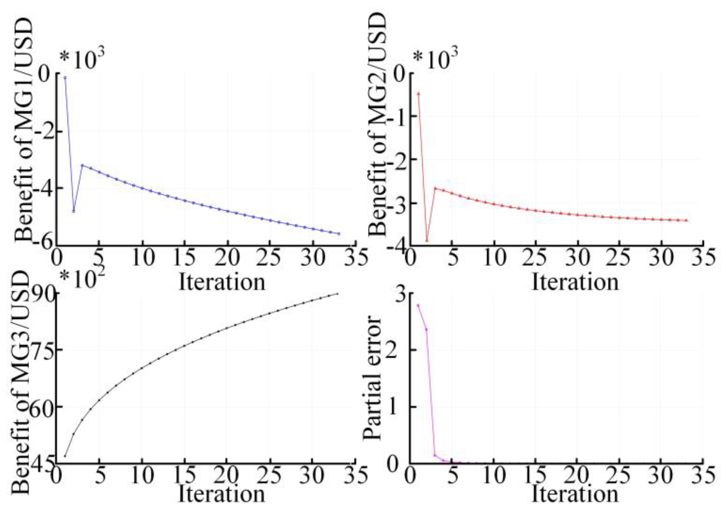
Figure 13 shows the transaction benefits among MGs and the results of the residual error iterative convergence. The ADMM algorithm requires 33 iterations to achieve convergence, the time is 53 s, and the convergence residual error is 10−3. Therefore, it shows that the ADMM algorithm proposed in this paper has good convergence performance and computational efficiency.
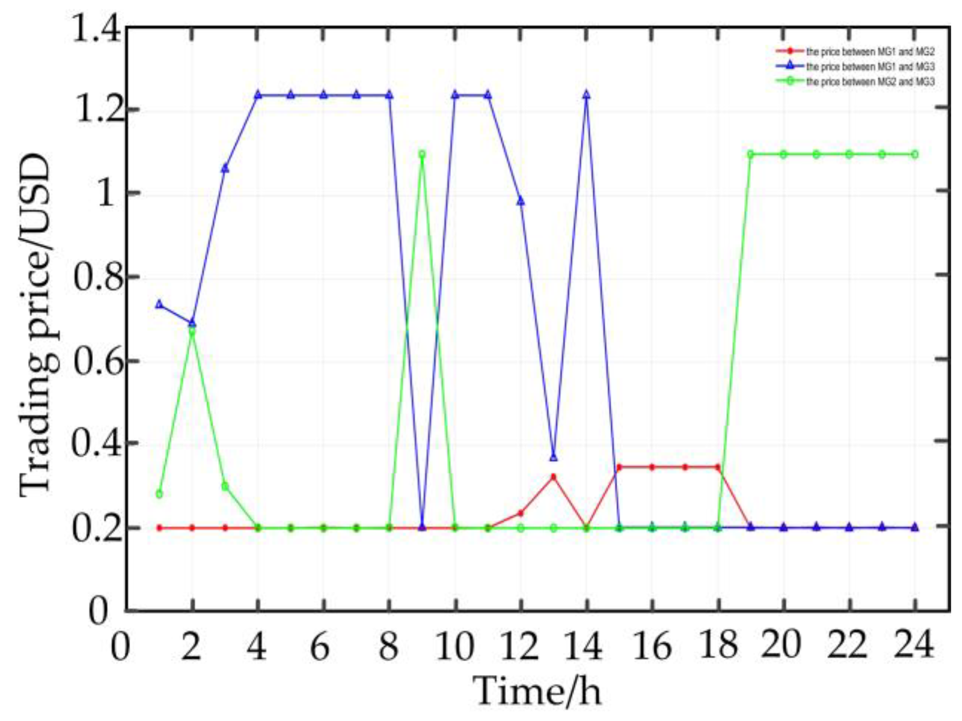
MG2 sells electricity to MG3 in Figure 9 from 9:00–15:00, for which the transaction price between MG2 and MG3 is relatively high at this time, as shown in Figure 14; MG2 purchases electric power from MG3 at 4:00–8:00, and the price between the two is at a low level. It can be seen that the transaction price among the MGs changes with the change in the electric power transaction.
Table 4 presents the running cost comparison of MC and multi-microgrids (MMG). MC is the model proposed in this paper; MMG is not considering constraints (35)–(36). It can be seen from the table that the operating cost of each MG in the MC are (USD 9660, USD 9628, USD 9628) less than that in MMG, which are (39.86%, 22.21%, 28.41%) lower. This shows that MC is beneficial to reducing the operating cost of each MG. Considering the influence of errors, the cost reduction of each MG is basically equal, which is 1/3 of the overall cost. It can be seen that the fairness of benefit distribution is facilitated by the Nash equilibrium.
5. Conclusions
The trading of carbon emissions and the high penetration of RE lead to the complexity of multi-energy MG systems. In addition, the utilization rate of RE is increasing, and this means that the MC must also be considered. In order to solve the problem of carbon emissions in MG, a joint IGDT dispatch strategy for MC considering the uncertainty of wind and PV is proposed in this paper. The P2G-CCS joint operation mechanism is considered in a single MG, and the bisection method is used to solve the purchase/sale electrical power price between the MC and SP. In addition, the risk avoidance strategy is adopted to consider the uncertainty of RE, and a non-probabilistic method, i.e., IDGT theory, is used to solve the robustness problem for MC. Finally, Nash negotiation is used to solve the transaction price among MGs. A simulation study is carried out on the MC considering SP, for which two cases are considered, including energy management with tiered carbon price and unified carbon price, and the comparison of carbon emissions and operating costs are given in two cases. The experimental results show that: (1) a reasonable carbon price can not only effectively and reasonably regulate the carbon trading market, but can also guide carbon emissions. (2) The uncertainty of RE is considered through weight coefficients and weighted summation, by which the robustness of the system is improved. (3) Considering the transaction among MGs by means of Nash bargaining, both the profits of the respective subjects and the interests of the whole system can be considered. Compared with MMG, it can also reduce the operating cost of each. Hydrogen energy is a direction of future comprehensive energy research, and this is also an indispensable discussion for hydrogen storage and hydrogen transaction prices.
In MC, the transaction prices of other energies, i.e., heat, gas, hydrogen, etc., can be considered in the future, as can the difference of carbon emission rights due to the differences of MG generator and load.
Author Contributions
Conceptualization, F.F.; methodology, F.F., H.C. and Q.S.; software, Q.S.; validation, F.F. and Q.S.; formal analysis, F.F. and H.C.; investigation, F.F. and Q.S.; resources, X.D.; data curation, F.F. and Q.S.; writing—original draft preparation, F.F. and X.D.; writing—review and editing, F.F., Q.S. and X.D.; visualization, X.D. and F.F.; supervision, F.F. and X.D.; project administration, F.F., Q.S., H.C. and X.D.; funding acquisition, Q.S. and X.D. All authors have read and agreed to the published version of the manuscript.
Funding
This research was funded by General Program of National Natural Science Foundation of China, grant number 61873336. This research was funded by The General Project of Natural Science Research of Jiangsu Province Colleges and Universities, grant number 19KJD560001.
Institutional Review Board Statement
Not applicable.
Informed Consent Statement
Not applicable.
Data Availability Statement
Not applicable.
Conflicts of Interest
The authors declare no conflict of interest.
Appendix A
Figure A1.
The process of solving the MC considering the SP by the bisection method.

Appendix B
This test system consists of the independent SP and three MGs.
MG1 consists of wind, PV, CHP, P2G-CCPP, GSHP, and ES alongside with residential loads, for which the specific dispatch model is
Equation (A1) includes the electric power, heat power balance constraints, and i = 1.
Equation (A2) shows that the fuel volume required by the MG1 is the difference between that consumed by CHP and generated by P2G.
The structure of MG2 is the same as MG3 alongside with wind, PV, GT, GB, P2G-CCS, ES, HS, and park loads. The specific dispatch models are
Equation (A3) illustrates the RE limit and the electric and heat power balance constraints; i = 1, 2.
The sum of the fuel consumed by GT and GB is the total fuel in the MG1,2, represented by Equation (A4).

Table A1.
Parameters of each unit in MG1.
| Parameter | Value | Parameter | Value | Parameter | Value |
| ηCHP | 0.75 | /kW | 3000 | /kW | 300 |
| /kW | 50 | /kW | 1200 | /kW | 0 |
| /kW | 1500 | λCHP | 0.3 | LHVCHP | 10.8 |
| /kW | 150 | /kW | 150 | SEmin | 100 |
| SEmax | 800 | 0.95 | 0.95 | ||
| ηP2G | 0.85 | LP2G | 3.9 | αCC | 0.78 |
| KCC | 0.269 | 500 | 400 | ||
| KGC | 0.78 | Kbuy | 0.56 | KHP | 3.8 |
Table A2.
Parameters of each unit in MG1 and MG2.
| Parameter | Value | Parameter | Value | Parameter | Value |
| 0.35 | 0.83 | /kW | 5000 | ||
| /kW | 800 | λGT | 0.35 | λGB | 0.9 |
| LHVTB | 9.7 | /kW | 300 | /kW | 300 |
| / | 0.98/0.98 | SEmax | 600 | STmax | 500 |
| /kW | 200 | /kW | 200 | / | 0.95 |
| ηP2G | 0.35 | LP2G | 3.9 | αCC | 0.78 |
| KCC | 0.269 | 500 | 400 | ||
| KGC | 0.78 | Kbuy | 0.56 |
Table A3.
Tiered carbon pricing.
| Interval | ||||||
|---|---|---|---|---|---|---|
| 0 | 1 | 2 | 3 | 4 | 5 | |
| Price (USD/t) | 2.5 | 2.5 | 3.34 | 4.01 | 4.68 | 5.35 |
References
- Sinha, R.K.; Chaturvedi, N.D. A Review on Carbon Emission Reduction in Industries and Planning Emission Limits. Renew. Sustain. Energy Rev. 2019, 114, 109304. [Google Scholar] [CrossRef]
- Parker, L. Climate Change: The European Union’s Emissions Trading System (EU-ETS); Congressional Research Service The Library of Congress: Washington, DC, USA, 2006. [Google Scholar]
- Gong, W.; Wang, C.; Fan, Z.; Xu, Y. Drivers of the peaking and decoupling between CO2 emissions and economic growth around 2030 in China. Environ. Sci. Pollut. Res. 2022, 29, 3864–3878. [Google Scholar]
- Niu, X.S.; Wang, J.Z.; Zhang, L.F. Carbon Price Forecasting System Based on Error Correction and Divide-conquer Strategies. Appl. Soft Comput. 2022, 112, 107935. [Google Scholar] [CrossRef]
- Wang, X.; Gong, Y.; Jiang, C. Regional Carbon Emission Management Based on Probabilistic Power Flow With Correlated Stochastic Variables. IEEE Trans. Power Syst. 2015, 30, 1094–1103. [Google Scholar] [CrossRef]
- Chen, Q.; Kang, C.; Xia, Q.; Zhong, J. Power Generation Expansion Planning Model Towards Low-Carbon Economy and Its Application in China. IEEE Trans. Power Syst. 2010, 25, 1117–1125. [Google Scholar] [CrossRef] [Green Version]
- Zhong, X.Q.; Zhong, F.; Liu, Y.; Yang, C.; Xie, S.L. Optimal Energy Management for Multi-energy Multi-microgrid Networks Considering Carbon Emission Limitations. Energies 2022, 246, 123428. [Google Scholar] [CrossRef]
- Chen, J.; Lu, B.; Hao, L. Research on Optimal Collaborative Method for Microgrid Environmental and Economic Dispatch in Grid-connected Mode. Int. J. Simul. Process Model. 2019, 14, 513. [Google Scholar] [CrossRef]
- Kanchev, H.; Colas, F.; Lazarov, V.; Francois, B. Emission Reduction and Economical Optimization of an Urban Microgrid Operation Including Dispatched PV-Based Active Generators. IEEE Trans. Sustain. Energy 2014, 5, 1397–1405. [Google Scholar] [CrossRef] [Green Version]
- Zhou, X.; Zhou, L.; Chen, Y.; Guerrero, J.M.; Luo, A. A microgrid cluster structure and its autonomous coordination control strategy. Int. J. Electr. Power Energy Syst. 2018, 100, 69–80. [Google Scholar] [CrossRef]
- Li, B.; Li, J. Probabilistic sizing of a low-carbon emission power system considering HVDC transmission and microgrid clusters. Appl. Energy 2021, 304, 117760. [Google Scholar] [CrossRef]
- Dong, X.; Li, X.S.; Cheng, S. Energy Management Optimization of Microgrid Cluster Based on Multi-Agent-System and Hierarchical Stackelberg Game Theory. IEEE Access 2020, 8, 206183–206197. [Google Scholar] [CrossRef]
- Wu, Q.; Xie, Z.; Li, Q.F.; Ren, H.B.; Yang, Y.W. Economic Optimization Method of Multi-stakeholder in A Multi-microgrid System Based on Stackelberg Game Theory. Energy Rep. 2022, 8, 345–351. [Google Scholar] [CrossRef]
- Lee, J.; Guo, J.; Choi, J.K.; Zukerman, M. Distributed energy trading in microgrids: A game-theoretic model and its equilibrium anal ysis. IEEE Trans. Ind. Electron. 2015, 62, 3524–3533. [Google Scholar] [CrossRef]
- Anoh, K.; Maharjan, S.; Ikpehai, A.; Zhang, Y.; Adebisi, B. Energy peer-to-peer trading in virtual microgrids in smart grids: A game-theoretic approach. IEEE Trans. Smart Grid 2020, 11, 1264–1275. [Google Scholar] [CrossRef]
- Ali, L.; Muyeen, S.M.; Bizhani, H.; Ghosh, A. Optimal Planning of Clustered Microgrid Using a Technique of Cooperative Game Theory. Int. J. Electr. Power Syst. Res. 2020, 183, 106262. [Google Scholar] [CrossRef]
- Guo, J.Q.; Tan, J.J.; Yang, L.; Gu, H.F.; Liu, X.; Cao, Y.; Yan, Q.; Xu, D.K. Decentralized Incentive-based Multi-energy Trading Mechanism for CCHP-based MG Cluster. Int. J. Electr. Power 2021, 133, 107138. [Google Scholar] [CrossRef]
- Khan, S.U.; Ahmad, I. A Cooperative Game Theoretical Technique for Joint Optimization of Energy Consumption and Response Time in Computational Grids. IEEE Trans. Papall. Distrib. 2009, 20, 346–360. [Google Scholar] [CrossRef] [Green Version]
- Xu, Y.T.; Ai, Q. Coordinated operation of microgrid and conventional generators considering carbon tax strategy. Autom. Electr. Power Syst. 2016, 40, 25–32. [Google Scholar]
- Wang, T.; Wang, X.; Gong, Y.; Jiang, C.W. Initial allocation of carbon emission permits in power systems. J. Mod. Power Syst. Clean Energy 2017, 5, 239–247. [Google Scholar] [CrossRef] [Green Version]
- Nguyen, T.A.; Crow, M.L. Stochastic optimization of renewable-based microgrid operation incorporating battery operating cost. IEEE Trans. Power Syst. 2015, 31, 2289–2296. [Google Scholar] [CrossRef]
- Zakariazadeh, A.; Jadid, S.; Siano, P. Smart microgrid energy and reserve scheduling with demand response using stochastic optimization. Int. J. Electr. Power Syst. Res. 2014, 63, 523–533. [Google Scholar] [CrossRef]
- Kuznetsova, E.; Ruiz, C.; Li, Y.F.; Ruiz, C.L.; Zio, E.R. Analysis of robust optimization for decentralized microgrid energy management under uncertainty. Int. J. Electr. Power Syst. Res. 2015, 64, 815–832. [Google Scholar] [CrossRef]
- Craparo, E.; Karatas, M.; Singham, D.I. A robust optimization approach to hybrid microgrid operation using ensemble weather forecasts. Appl. Energy 2017, 201, 135–147. [Google Scholar] [CrossRef]
- Li, Y.; Wang, P.; Gooi, H.B.; Ye, J.; Wu, L. Multi-objective optimal dispatch of microgrid under uncertainties via interval optimization. IEEE Trans. Smart Grid 2017, 10, 2046–2058. [Google Scholar] [CrossRef]
- Zhang, X.; Son, Y.; Cheong, T.; Choi, S.Y. Affine-arithmetic-based microgrid interval optimization considering uncertainty and battery energy storage system degradation. Energy 2022, 242, 123015. [Google Scholar] [CrossRef]
- Cao, Y.; Li, D.; Zhang, Y.; Tang, Q.H.; Khodaei, A.; Zhang, H.L. Optimal energy management for multi-microgrid under a transactive energy framework with distributionally robust optimization. IEEE Trans. Smart Grid 2021, 13, 599–612. [Google Scholar] [CrossRef]
- Cai, S.; Xie, Y.; Wu, Q.; Zhang, M.L.; Jin, X.L.; Xiang, Z.R. Distributionally robust microgrid formation approach for service restoration under random contingency. IEEE Trans. Smart Grid 2021, 12, 4926–4937. [Google Scholar] [CrossRef]
- Hu, J.X.; Li, H.G. A Transfer Learning-based Scenario Generation Method for Stochastic Optimal Scheduling of Microgrid with Newly-built Wind Farm. Renew. Energy 2022, 185, 1139–1151. [Google Scholar] [CrossRef]
- Morales, J.M.; Conejo, A.J.; Perez-Ruiz, J. Short-term Trading for a Wind Power Producer. IEEE Trans. Power Syst. 2010, 25, 554–564. [Google Scholar] [CrossRef]
- Huang, C.; Yue, D.; Deng, S.; Xie, J. Optimal scheduling of microgrid with multiple distributed resources using interval optimization. Energies 2017, 10, 339. [Google Scholar] [CrossRef] [Green Version]
- Yang, D.; Jiang, C.; Cai, G.W.; Yang, D.Y.; Liu, X.J. Interval method based optimal planning of multi-energy microgrid with uncertain renewable generation and demand. Appl. Energy 2020, 277, 115491. [Google Scholar] [CrossRef]
- Saki, R.; Rokrok, E.; Abedini, M.; Doostizadeh, M. Risk-averse Microgrid Cluster Switching Approach for Improving Distribution System Characteristics Considering Uncertainties of Renewable Energy Resources. IET Renew. Power Gener. 2020, 14, 1997–2006. [Google Scholar] [CrossRef]
- Ahmadi, S.E.; Rezaei, N. An IGDT-based Robust Optimization Model for Optimal Operational Planning of Cooperative Microgrid Clusters: A Normal Boundary Intersection Multi-objective Approach. Int. J. Electr. Power 2021, 127, 106634. [Google Scholar] [CrossRef]
- Hu, J.Z.; Wang, X.; Jiang, Z.W.; Cong, H. Optimal Tiered Carbon Price of Power System Considering Equilibrium of Regional Carbon Emission. Autom. Electr. Power Syst. 2020, 44, 98–107. (In Chinese) [Google Scholar]
- Fan, S.; Ai, Q.; Piao, L. Bargaining-based cooperative energy trading for distribution company and demand response. Appl. Energy 2018, 226, 469–482. [Google Scholar] [CrossRef]
Figure 1.
Sample MC system structure.

Figure 2.
Interval tiered carbon price.

Figure 3.
P2G and CCS joint operation structure.

Figure 4.
Flow chart of IGDT multi-source joint dispatching strategy of MC.

Figure 5.
The power of RE: (a) PV; (b) wind.

Figure 6.
Output dispatch of MG1: (a) electric; (b) heat.

Figure 7.
Output dispatch of MG2: (a) electric; (b) heat.

Figure 8.
Output dispatch of MG3: (a) electric; (b) heat.

Figure 9.
Electric power trading among MGs.

Figure 10.
Electric trading price among MGs: (a) MG1; (b) MG2; (c) MG3.

Figure 11.
Comparison of IGDT result in two cases.

Figure 12.
Carbon emission in two prices: (a) MG1; (b) MG2; (c) MG3.

Figure 13.
Convergence of the ADMM algorithm.

Figure 14.
Trading price among MGs.

Table 1.
Operating cost (USD) for two algorithms.
| Parameter | MG1 | MG2 | MG3 | SP | Iteration |
|---|---|---|---|---|---|
| Bisection Algorithm | 24,231 | 43,348 | 33,894 | 13,718 | 8 |
| Golden cut Algorithm | 25,382 | 44,927 | 34,833 | 14,180 | 11 |
Table 2.
IGDT robust dispatch results with different weight coefficient combinations.
| Parameter | IGDT Robust Dispatching Result | ||
|---|---|---|---|
| (βPV, βW) | αPV | αW | ψ |
| (1, 1) | 0.7868 | 0.6869 | 1.3025 |
| (1, 2) | 0.7868 | 0.3279 | 1.4425 |
| (1, 4) | 0.7868 | 0.1968 | 1.5739 |
| (1, 8) | 0.7868 | 0.1182 | 1.7374 |
Table 3.
Operating costs in two prices.
| Operating Cost (USD) | Interval Price | Uniform Price | ||||
|---|---|---|---|---|---|---|
| MG1 | MG2 | MG3 | MG1 | MG2 | MG3 | |
| Cgrid | 12,138 | 17,858 | 10,911 | 14,361 | 19,424 | 10,959 |
| Cfuel | 10,354 | 20,978 | 19,377 | 11,383 | 20,167 | 19,389 |
| CES | 22 | 45 | 34 | 23 | 52 | 47 |
| CV | 1717 | 4467 | 3572 | 2416 | 4386 | 3203 |
| The total operating cost | 24,231 | 43,348 | 33,894 | 28,183 | 44,029 | 33,598 |
Table 4.
Comparisons of operation costs for MC and MMG.
| Operation Cost (USD) | |||
|---|---|---|---|
| MG1 | MG2 | MG3 | |
| MC | 24,231 | 43,348 | 33,894 |
| MMG | 33,891 | 52,976 | 43,522 |
Publisher’s Note: MDPI stays neutral with regard to jurisdictional claims in published maps and institutional affiliations. |
© 2022 by the authors. Licensee MDPI, Basel, Switzerland. This article is an open access article distributed under the terms and conditions of the Creative Commons Attribution (CC BY) license (https://creativecommons.org/licenses/by/4.0/).
Share and Cite
MDPI and ACS Style
Feng, F.; Du, X.; Si, Q.; Cai, H. Hybrid Game Optimization of Microgrid Cluster (MC) Based on Service Provider (SP) and Tiered Carbon Price. Energies 2022, 15, 5291. https://doi.org/10.3390/en15145291
AMA Style
Feng F, Du X, Si Q, Cai H. Hybrid Game Optimization of Microgrid Cluster (MC) Based on Service Provider (SP) and Tiered Carbon Price. Energies. 2022; 15(14):5291. https://doi.org/10.3390/en15145291
Chicago/Turabian StyleFeng, Fei, Xin Du, Qiang Si, and Hao Cai. 2022. "Hybrid Game Optimization of Microgrid Cluster (MC) Based on Service Provider (SP) and Tiered Carbon Price" Energies 15, no. 14: 5291. https://doi.org/10.3390/en15145291
Note that from the first issue of 2016, this journal uses article numbers instead of page numbers. See further details here.