Profit Maximization with Imbalance Cost Improvement by Solar PV-Battery Hybrid System in Deregulated Power Market

Abstract

The changeable nature of renewable sources creates difficulties in system security and stability. Therefore, it is necessary to study system risk in several power system scenarios. In a wind-integrated deregulated power network, the wind farm needs to submit the bid for its power-generating quantities a minimum of one day ahead of the operation. The wind farm submits the data based on the expected wind speed (EWS). If any mismatch occurs between real wind speed (RWS) and expected wind speed, ISO enforces the penalty/rewards to the wind farm. In a single word, this is called the power market imbalance cost, which directly distresses the system profit. Here, solar PV and battery energy storage systems are used along by the wind farm to exploit system profit by grasping the negative outcome of imbalance cost. Along with system profit, the focus has also been on system risk. The system risk has been calculated using the risk assessment factors, i.e., Value-at-Risk (VaR) and Cumulative Value-at-risk (CVaR). The work is performed on a modified IEEE 14 and modified IEEE 30 bus test system. The solar PV-battery storage system can supply the demand locally first, and then the remaining power is given to the electrical grid. By using this concept, the system risk can be minimized by the incorporation of solar PV and battery storage systems, which have been studied in this work. A comparative study has been performed using three dissimilar optimization methods, i.e., Artificial Gorilla Troops Optimizer Algorithm (AGTO), Artificial Bee Colony Algorithm (ABC), and Sequential Quadratic Programming (SQP) to examine the consequence of the presented technique. The AGTO has been used for the first time in the risk assessment and alleviation problem, which is the distinctiveness of this work.

1. Introduction

According to the norm, electricity was a monopoly owned by regional powers that had both production and distribution [1]. Countries allow the status quo to exist in the equivalent exchange for being provided a cut in the cost of service. This system was adopted even though it had a huge flaw, which was the potential to influence state policymakers. To break down this monopoly environment, deregulation was introduced over a centralized action taken over many years. Deregulation refers to the breakdown of monopolies at the state level, and these monopolies are sold or transferred to third parties [2]. The regulation resulted in the monopoly of the production and distribution of electricity by electric utility companies, which, in extension, led to a monopoly over the wholesale market. Additionally, by introducing deregulation, the monopoly was reduced.

The introduction of deregulation was an unintended move on the part of the government. It started in the 1970s in the form of an unintentional act called the Public Utility Regulatory Policy Act (PURPA). PURPA started as an act to encourage alternative sources of energy [3]. After these initiatives, most countries are moving toward the implementation of deregulation in their electrical networks to provide more economical facilities to their citizens [4,5].

With the continuous deprivation in the quantity of coal and fossil fuels throughout the world, power-generating stations are thinking about unconventional sources [6]. The uncertain nature of renewable energy creates issues such as energy management [7] and protection [8] in renewable combined power systems. The renewable addition of the present thermal power plant in the day-ahead market is very complicated, but the consumer experiences the benefit [9]. Some work has been accomplished by researchers in this field in recent years.

Paper [10] portrays the significance of renewable additions in the electricity market by the lower structure disruptions. Xing et al. [11] demonstrated that variable renewable electricity (VRE) performs a vital role in global decarbonization. The incorporation expenses of solar and wind on the demand and source sides by the economic dispatch model are discussed by the author. Life cycle assessment based on the performance degradation of solar panels has been discussed in [12]. The authors discussed how installed capacity decreases after deployment in the field and how this affects overall finances. Shujin et al. [13] discussed the decrement of renewable resources due to the overconsumption of renewable electricity in day-to-day life. In [14], the author states that the available transfer capability (ATC) performs a significant part in the deregulated market, and knowing it in advance can help to use the transmission network more efficiently. The authors of [15] displayed an arrangement of conventional and non-conventional systems with energy storage equipment to learn the impression of renewable uncertainties. The work in [16] showed how virtual power plants can be utilized to collectively manage renewable energy-based resources for efficient use. Reddy et al. [17] presented a methodology of renewable combined systems to exploit system safety and economic profit. In [18,19], the advantages of CAES in the system economy have been presented for the electricity market. In [20], the work aimed to decouple the focused solar energy output by CAESs and to model the MCP with the proposed offering strategies.

Chang et al. [21] discussed the influence of wind turbine generators (WTG) on system operation using Evolutionary Particle Swarm optimization (EPSO). A risk-mitigation bidding plan considering CVaR has been elucidated in [22]. Matevosyan et al. [23] projected a bidding strategy to lessen the imbalance of pricing in the wind-integrated short-term deregulated power market. In [24], a technique is proposed by the author for evaluating the effect of the unpredictable nature of wind flow in a wind combined competitive electrical system.

The authors of [25] introduced a novel optimization system to regulate the optimum generator schedule and involve load response to reduce the risk of transmission overloading burden in the forecasting power market. Rubin et al. [26] illustrated an equilibrium modeling technique to examine the impression of integrating wind power in a deregulated market. Das et al. [27] proposed risk mitigation methods in a wind-incorporated competitive power system using flexible AC Transmission Systems (FACTS) devices. The authors of [28] showed the importance of wind power incorporation in the system economy in deregulated markets. Khamees et al. [29] presented a key method of optimum power flow in a wind-incorporated electrical system to optimize the system fuel cost. Paper [30] depicts a scheduling technique for the best capacity sharing of a solar PV, wind farm, and pumped hydro storage system. The works in [31,32] presented a method for risk curtailment using FACTS devices and pumped hydro storage plants simultaneously in a wind-incorporated system.

From the detailed studies, it can be seen that several risks and financial mitigation work have been completed earlier, but there are still some scopes that have been done in this paper.

In the electricity market, wind farms need to submit the power generation scenario for the next day to ISO, a minimum day ahead of operation. Based on the acquiesced bid for the wind power plant, ISO arranged the power generation scheduling for all present generating stations. Due to the vagueness of the wind, there is a chance of not satisfying the arrangement of power from the wind plant. The ISO imposes an imbalance cost on the wind farm when a violation occurs in the electricity market. When real wind power (RWP) is more than expected wind power (EWP), then ISO grants rewards to the wind plant for the extra power sourced to the grid. ISO enforces a penalty on the wind plant if the EWP is more than the RWP. The negative imbalance cost (i.e., penalty) minimizes the system profit. Therefore, it is necessary to reduce the damaging effect of imbalance costs by reducing the mismatching amount between real and expected power generation from the wind farm to maintain system profit. Solar PV and battery energy storage can play an important role in this situation by providing additional power. The key highlights of this work are:

• Twenty scenarios with different system abnormalities (i.e., bus failure, transmission line failure, generator failure, sudden load increment, etc.) have been created to verify the success of the presented work. The VaR and CVaR have been calculated for all scenarios based on two system parameters: nodal pricing (NP) and transmission line flow (LF).
• The wind farm placement has been performed to reduce the system risk and exploit the system economics.
• Solar PV and battery storage are used to maximize the system profit while minimizing the harmful consequences of imbalance costs in the system. A comparative study has been performed using AGTO, ABC, and SQP to check the success of renewable integration in the electricity market in terms of operating cost and system risk.
• The AGTO has been used for the first time in the risk assessment and alleviation problem, which is the distinctiveness of this work.

2. Mathematical Formulations

This unit contains detailed studies on the mathematical formulation of wind power and risk assessment tools.

2.1. Wind Power Quantity and Investment Cost

The wind flows are very uncertain. This is changing every moment. The quality of wind power generation depends on the air density ($\mathsf{\rho }$), efficiency of wind turbine (η), swept area of the wind turbine (A), and wind speed (WS). The generated wind power (GWP) is formulated as follows [33]:

$$\mathrm{G}\mathrm{W}\mathrm{P}=\frac{1}{2}\mathsf{\rho }·\mathrm{A}·\mathsf{\eta }·{(\mathrm{W}\mathrm{S})}^3$$

(1)

All the parameters are fixed for a particular place; only wind speed varies at every moment. In this case, the considered wind farm parameters are as follows: $\mathsf{\rho }$ = 1.225 kg/m³, η = 0.49, wind turbine rotor radius (r) = 40 m. Real-time wind speed data are not obtainable at the height of the wind turbine. In India, real-time wind speed data are available at a height of 10 m from the ground level. Under maximum conditions, the wind turbine height is 120 m. Therefore, the calculation is required to determine the wind speed at the desired height [33]:

$$\frac{\mathrm{W}{\mathrm{V}}_{{}_{\mathrm{h}}}}{\mathrm{W}{\mathrm{V}}_{10}}={\left(\frac{\mathrm{h}}{10}\right)}^{\mathrm{N}}$$

(2)

Here, WV_h and WV₁₀ are the wind speed at heights ‘h’ and 10 m. N is the Hellman co-efficient (1/7).

2.2. Risk Assessment Parameters (VaR and CVaR)

VaR and CVaR have been chosen as the risk assessment parameters in this work. Other risk assessment tools can also be used, but based on the efficiencies and feasibilities in the field of power systems, these tools have been considered here. CVaR has greater numerical properties than other risk valuation tools. CVaR is also known as a coherent risk measurement tool. The CVaR of a set is a continuous function, whereas the other tools may be discontinuous. The CVaR deviation is a robust contestant to the standard deviation. Under maximum conditions, the standard deviation can be substituted by a CVaR deviation to obtain better results. In risk management, CVaR functions can be performed more efficiently than the other risk assessment tools. CVaR can be optimized with linear programming methods, whereas VaR and other risk-assessing tools are relatively difficult to enhance. CVaR delivers a suitable picture of risks replicated in extreme tails. This is a very significant property if extreme tail losses are properly projected. For these reasons, CVaR is chosen as the risk assessment tool in this work.

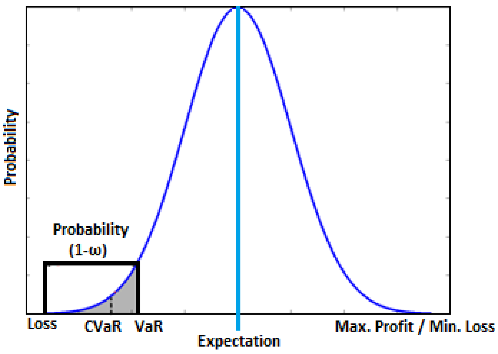
Both the considered assessment tools work based on probabilistic studies and the confidence level of assurance (ɷ). The confidence level of occurrence is 98% for measuring the values of VaR and CVaR. VaR represents the smallest loss with loss amount of (1 − ɷ) percentile but CVaR illustrates the average loss mechanisms. m(x,y) is the loss mechanism related to the decision vector P, which is taken from a definite subset x of $\dot{Q}$ and the random vector y in $\dot{Q}$. The probability of loss components m(x,y) is indicated by n(y), which must be ranged with a threshold limit (ξ) [34]:

$$\beta \left(x,\xi \right)={{\displaystyle \int }}_{m\left(x,y\right)\le \xi }n\left(y\right)d\xi$$

(3)

The assurance level-based VaR and CVaR are as follows [34]:

$${\xi }_p\left(x\right)=min\left\{\xi ϵ\dot{Q}:\beta \left(x,\xi \right)\right\}$$

(4)

$${\theta }_p\left(x\right)=\frac{1}{1-\mathsf{ɷ}}\left[({{\displaystyle \sum }}_{c=1}^{C_a}\left(n_c-\mathsf{ɷ}\right)p_{c_a}+{{\displaystyle \sum }}_{c=c_a}^T{n}_c{p}_c\right]$$

(5)

Here, T is the number of trials composed under numerous conditions.

Figure 1 shows a graphical illustration of the risk assessment factors. The maximum negative values of the parameters portray the maximum system risk. Therefore, it is necessary to transfer toward the right-hand side to lessen system loss and system risk.

3. Optimization Techniques

Some nature-inspired optimization techniques are popular in today’s world due to their efficacy in solving stability issues for renewable incorporated systems [35]. These include frequency stability [36,37], cost minimization [38], and energy and storage otmimization [39,40,41]. This unit shows the particulars of the considered optimization techniques, i.e., AGTO, ABC, and SQP. Here, SQP is the linear optimization technique, whereas ABC and AGTO are advanced optimization tools. Other optimization techniques can also be used, but these algorithms are chosen randomly for comparative studies. The AGTO algorithm has been proposed in 2021. Therefore, its application has been displayed here to check the efficiencies of the proposed approach along with the relatively old optimization technique ABC and the linear optimization technique SQP.

The following features of metaheuristic algorithms have created interest among the researchers over the analytic methods: (i) the accuracy is advanced than that of the analytical approaches, (ii) the iteration number is less for metaheuristic methods, (iii) the processes can be simply adapted for the two diode models of solar PV systems with metaheuristic algorithms, and (iv) the recital of the parameters abstraction can be enhanced using meta heuristic algorithms.

The concept of AGTO has been taken from [42], whereas [43] provides a detailed concept of ABC optimization algorithms. Here, MATPOWER software has used to solve the OPF problem using SQP. The SQP is also the same as a simplification of the Newton Raphson Technique, in which non-linear controlled optimization difficulties are answered in steps wise to determine the OPF.

4. Problem Formulation

The aim of this work is to exploit the system profit and diminish the system risk by best location of wind farms, solar PV, and battery storage. Solar PV and batteries are considered backup power sources that are used to lessen the negative influence of imbalance costs in the electricity market environment. The second objective is to impact the valuation of imbalance costs on system profit in a wind-incorporated deregulated power network and to exploit the system profit using the best action of a solar PV-battery storage system.

Objective Function 1:

$$\mathrm{Maximize},P\left(t\right)=R\left(t\right)-GC\left(t\right)$$

(6)

Here, P(t), R(t) and GC(t) are system profit, revenue earned and generation cost at time ‘t’ 1 in $/h.

$$R\left(t\right)={{\displaystyle \sum }}_{m=1}^{NG}P{G}_r\left(m,t\right)\cdot {\lambda }_{loc}\left(m,t\right)$$

(7)

$$GC\left(t\right)=G{C}_{Th}\left(t\right)+G{C}_W\left(t\right)$$

(8)

$$G{C}_{Th}\left(t\right)={{\displaystyle \sum }}_{m=1}^{N_g}\left(a_m+b_m·P{G}_r\left(m,t\right)+c_m·P{G}_r^2\left(m,t\right)\right)$$

(9)

Here, ‘PGr(m,t)’ is the power generated capacity with RWS at time ‘t’ for bus-m, ‘${\lambda }_{loc}\left(m,t\right)$’ is the retailing price of generator-m. The system generation cost has two parts: thermal generation cost ($G{C}_{Th}\left(t\right)$) and wind generation cost ($G{C}_W\left(t\right)$). NG is the generator number that is linked to the system. ‘a_m’, ‘b_m’ and ‘c_m’ are the cost co-efficient of generation units.

The scientific expression of the risk-associated objective function is as follows [34]:

$$\mathrm{Max}. {\xi }_p\left(x\right)=min\left\{\xi ϵ\dot{Q}:\beta \left(x,\xi \right)\right\}$$

(10)

$$\mathrm{Max}. {\theta }_p\left(x\right)=\frac{1}{1-\mathsf{ɷ}}\left[({{\displaystyle \sum }}_{c=1}^{C_a}\left(n_c-\mathsf{ɷ}\right)p_{c_a}+{{\displaystyle \sum }}_{c=c_a}^T{n}_c{p}_c\right]$$

(11)

Here, the VaR and CVaR have not been included in the optimization techniques directly. After applying the optimization techniques for profit maximization, the system data has been collected. Then, VaR and CVaR are calculated using that data. From Figure 1, it is observed that the system risk will be diminished when VaR and CVaR rise. Therefore, this objective function is taken as a maximization problem.

Objective Function 2:

In this objective function, the concept of imbalance has been introduced along with the first objective function. Now, the scientific expression of this objective is as:

$$\mathrm{Maximize},P\left(t\right)=R\left(t\right)+IC\left(t\right)-GC\left(t\right)$$

(12)

Here, IC(t) is the system imbalance cost at time ‘t’. This is generated due to a mismatch in bidding quantities and actual generated quantities of wind power. ISO imposes a penalty on wind farms for their deficit power supply conditions. Furthermore, ISO provides a reward if surplus power has been supplied to the grid by the wind farm. Imposing a penalty on the wind farm creates ‘−ve’ imbalance cost, and rewards provided to the wind firm create ‘+ve’ imbalance cost. The solar PV and battery energy storing systems can play a dynamic role in this situation. By providing extra power to the wind farm at the required time, a solar PV-battery hybrid system can alleviate the negative effect of imbalance costs and can exploit the system profit. The mathematical expression of the system imbalance cost is as follows:

$$IC\left(t\right)={{\displaystyle \sum }}_{m=1}^{NG}\left(R_S\left(t\right)+R_D\left(t\right)·{\left(\frac{P{G}_e\left(m,t\right)}{P{G}_r\left(m,t\right)}\right)}^2\right)·\left(P{G}_r\left(m,t\right)-P{G}_e\left(m,t\right)\right)$$

(13)

$$R_D\left(t\right)=\left(1+\beta \right)·{\lambda }_{loc}\left(m,t\right),R_S\left(t\right)=0 ifP{G}_e\left(m,t\right)>P{G}_r\left(m,t\right)$$

(14)

$$R_S\left(t\right)=\left(1-\beta \right)·{\lambda }_{loc}\left(m,t\right),R_D\left(t\right)=0 ifP{G}_e\left(m,t\right)<P{G}_r\left(m,t\right)$$

(15)

$$R_S\left(t\right)=R_D\left(t\right)=0 otherwise$$

(16)

Here, ‘$R_S\left(t\right)$’ and ‘$R_D\left(t\right)$’ are surplus charge rate and deficit charge rate, ‘PG_e(m,t)’, ‘PG_r(m,t)’ are generated power quantities with expected and real wind speed respectively. ‘β’ is the system imbalance cost co-efficient. In this work, ‘β’ is presumed to be 0.8, as this value varies from 0 to 1 [33].

• Constraints:

Equality and inequality constraints have been taken to solve the OPF problem.

$${{\displaystyle \sum }}_{m=1}^{NG}P{G}_r+GWP-P_{loss}-P_L=0$$

(17)

$$P_{loss}={{\displaystyle \sum }}_{n=1}^{N_{TL}}{G}_n\left[{\left|V_p\right|}^2+{\left|V_q\right|}^2-2\left|V_p\right|\left|q\right|cos\left({\delta }_p-{\delta }_q\right)\right]$$

(18)

$$P_m-{{\displaystyle \sum }}_{k=1}^{NB}\left|V_m{V}_k{Y}_{mk}\right|cos\left({\theta }_{mk}-{\delta }_m+{\delta }_k\right)=0$$

(19)

$$Q_m+{{\displaystyle \sum }}_{k=1}^{NB}\left|V_m{V}_k{Y}_{mk}\right|sin\left({\theta }_{mk}-{\delta }_m+{\delta }_k\right)=0$$

(20)

$$V_m^{min}\le V_m\le V_m^{max} m=1,2,3\dots NB$$

(21)

$${\varnothing }_m^{min}\le {\varnothing }_m\le {\varnothing }_m^{max} m=1,2,3\dots NB$$

(22)

$$T{L}_l\le T{L}_l^{max} l=1,2,3\dots N_{TL}$$

(23)

$$P_{Gm}^{min}\le P_{Gm}\le P_{Gm}^{max} m=1,2,3\dots NB$$

(24)

$$Q_{Gm}^{min}\le Q_{Gm}\le Q_{Gm}^{max} m=1,2,3\dots NB$$

(25)

‘P_loss’ and ‘PL’ are transmission line loss and system loads. N_TL is the number of transmission lines. Y_mk and θ_mk are the magnitude and angle of the m x n-th element of bus admittance matrix. The voltage magnitude are |V_p|, |V_q|, and V_k for bus p, q, and k. P_m and Q_m are active and reactive power at bus-m. Gn is transmission line conductance. The voltage angles are δm and δk for bus ‘m’ and ‘k,’ respectively. ϕ_m^min and ϕ_m^max are the least and most extreme angle limits at bus ‘m’. V_m^min and V_m^max are lesser and greater voltage bounds. TL_l and TL_l^max are actual and extreme line flows. PG_m^min, PG_m^max, QG_m^min, and QG_m^max are lesser and higher real and reactive power limits. NB is the bus number.

The step-by-step process of the presented work is as follows:

Step 1:

Read all system information for the considered test system.

Step 2:

Generate 20 different scenarios for creating system congestion by bus outage, line outage, generator outage, and load increment.

Step 3:

Calculate the system generation cost, revenue, profit, and system risk (based on NP and LF) without wind placement in the system.

Step 4:

Choose the 2 most severe scenarios with the base case from the 20 scenarios based on the values of risk assessment tools.

Step 5:

Collect hourly real and expected wind speed data from Kolhapur and Mumbai.

Step 6:

Calculate wind power generation and wind power costs.

Step 7:

Calculate the system generation cost, revenue, profit, and system risk (based on NP and LF) with wind placement in the system.

Step 8:

Calculate the imbalance cost considering wind speed data and compare the system profit with and without the imbalance cost.

Step 9:

Place solar PV and battery energy storage systems and check system risk and system profit.

Step 10:

Compare system risk and system economy with different optimization techniques.

5. Implementation of the Proposed Approach

A modified IEEE 14-bus and modified IEEE 30-bus system is deliberated to explore the effect in this work. The base MVA is 100 for the system, and bus no. 1 is the reference bus for the IEEE 14-bus system [28,34]. SQP, AGTO, and ABC algorithms have been used to solve the optimal power flow problem. Different scenarios have been taken to examine system performance.

• Case 1: Scenario Generation and Finding the Worst Case Based on System Risk (Modified IEEE 14-bus System)

Twenty different scenarios have been generated considering the different types of system instabilities, such as bus failure, generator failure, transmission line failure, and sudden increment of system load. System risk and system generation costs have been calculated on behalf of every chosen case using SQP.

Table 1. Economic parameters and system risk of the system.

Scenario No.	Details	System Generation Cost ($/h)	Revenue ($/h)	Profit ($/h)	VaR on NP	CVaR on NP	VaR on LF	CVaR on LF
1	Base Case	899.09	1226.19648	327.1065	−0.3897	−0.5996	−0.7529	−0.7926
2	Line outage (2–3)	952.57	1368.904	416.334	−0.4719	−0.726	−0.9598	−1.0664
3	Line outage (4–5)	967.36	1405.72038	438.3604	−0.5295	−0.8146	−0.752	−0.8356
4	Generator outage (2)	1094.92	1784.70386	689.7839	−0.604	−0.829	−0.8012	−0.8433
5	Bus_4 (15%)	935.66	1286.4382	350.7782	−0.4009	−0.6168	−0.7536	−0.7932
6	Bus_6 (15%)	906.36	1235.63664	329.2766	−0.3896	−0.5993	−0.7527	−0.7923
7	Line outage (13–14)	1024.48	1583.71197	559.232	−0.8787	−1.3519	−0.9069	−1.0076
8	Bus_11 (15%)	1094.94	1783.79553	688.8555	−0.9822	−1.5111	−0.7702	−0.8108
9	Bus_14 (15%)	1115.49	1821.69013	706.2001	−10.978	−16.889	−0.9718	−1.0229
10	Bus_10 (15%)	1113.42	1817.68268	704.2627	−10.153	−15.623	−0.9901	−1.0422
11	Bus_9 (11%)	1156.23	1919.31698	763.087	−6.4408	−9.9089	−0.8375	−0.8816
12	Bus_2 (11%)	909.85	1242.168	332.318	−0.3817	−0.5872	−0.7532	−0.7929
13	Line outage (1–5)	918.75	1266.423	347.673	−0.4597	−0.7073	−0.7533	−0.837
14	Line outage (10–11)	986.68	1486.184	499.504	−0.8845	−1.3608	−0.9218	−1.0243
15	Line outage (6–12)	902.7	1237.829	335.129	−0.3932	−0.6049	−0.7476	−0.8307
16	Bus_12 (14%)	900.32	1227.485	327.165	−0.3917	−0.6026	−0.7837	−0.8249
17	Bus_3 (14%)	995.92	1405.286	409.366	−0.5162	−0.7941	−0.7536	−0.7933
18	Line outage (12–13)	897.04	1224.889	327.849	−0.3923	−0.6036	−0.7469	−0.8299
19	Line outage (9–14)	895.84	1218.687	322.847	−0.3919	−0.6029	−0.7595	−0.8439
20	Line outage (12–13)	936.58	1332.214	395.634	−0.5027	−0.7734	−0.9511	−1.0567

shows the system economic parameters and system risk for the considered scenarios, along with the base case. The risk assessment tools (i.e., VaR and CVaR) are operated based on system nodal prices (NP) and power flow in the transmission lines (LF).

Table 1 shows that scenarios 9 and 10 are the most severe risky scenario due to their negative highest values of VaR and CVaR, which indicate the minimum profit and maximum losses of the system. The system generation cost depends on several system parameters, including transmission line congestion. When the system is riskier, then the generation cost is also high due to the high congestion cost.

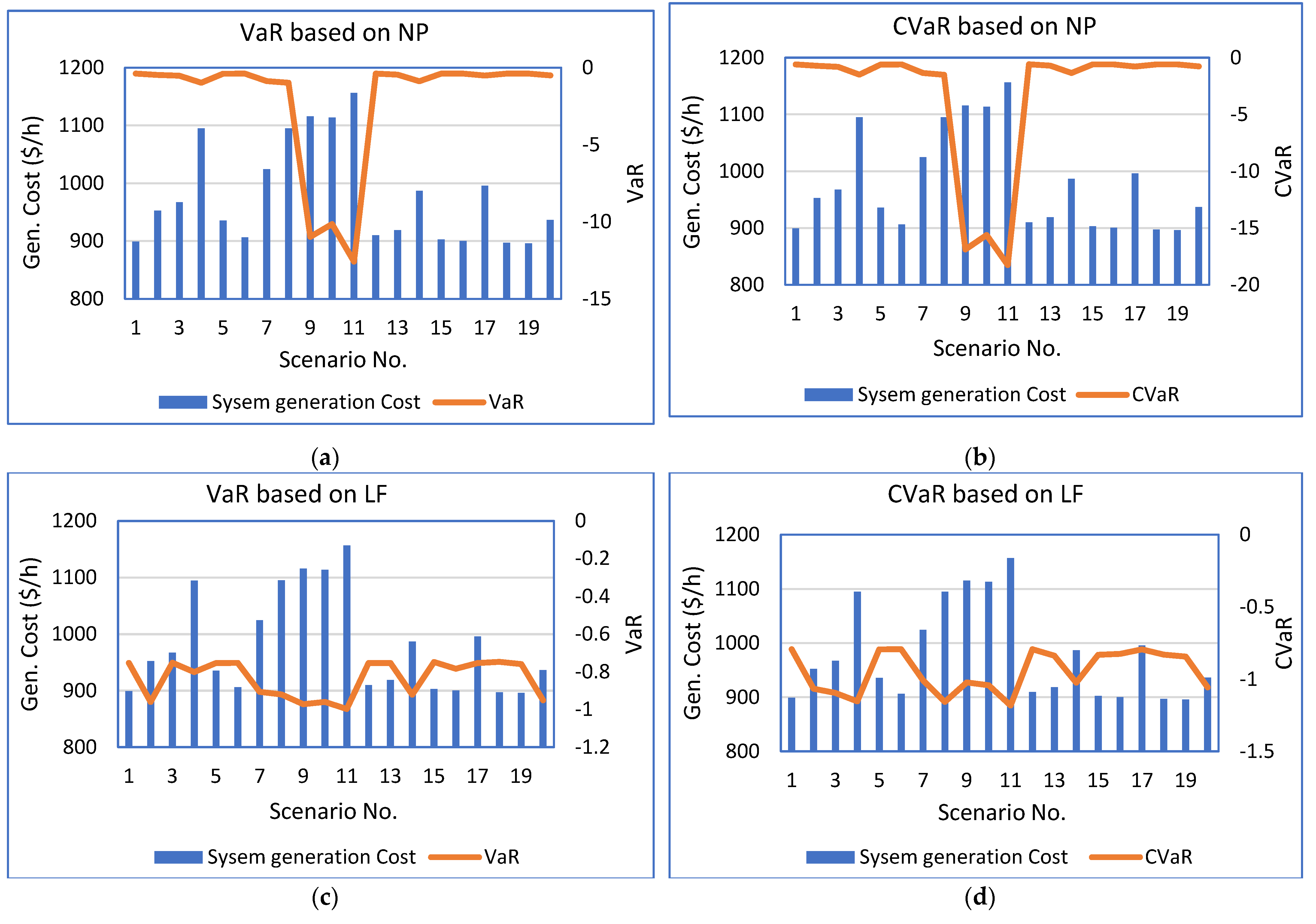
Figure 2 depicts the relation between system generation cost with risk assessment tools for all considered cases. For further study of this work, the most 2 risky scenarios along with the base conditions have been considered. If solar PV and battery storage provide better results for the worst cases, then this method will also provide better results for other cases. Therefore, only three cases have been considered for further studies.

• Step 2: System Economy (without imbalance cost) and Risk with Wind Farm Integration (Modified IEEE 14-bus system)

Wind speed varies in every period throughout the world. Considering the flexible nature of wind flow, two places have been considered in India (i.e., Kolhapur and Mumbai) for real-time problem solving. The wind speed data has been taken for 4 different times (6 AM, 12 noon, 6 PM and 12 midnight) for both considered places. Both real and expected wind speed data have been considered for all cases.

Table 2. Real-time Wind Speed Data [44].

Sl. No.	Details	Kolhapur		Mumbai
		RWS (km/h)	EWS (km/h)	RWS (km/h)	EWS (km/h)
1	Base Case_(00.00 h)	8	9	7	8
2	Base Case_(06.00 h)	9	11	8	9
3	Base Case_(12.00 h)	13	13	11	13
4	Base Case_(18.00 h)	8	7	9	9
5	Bus_14 (15%)_(00.00 h)	8	9	7	7
6	Bus_14 (15%)_(06.00 h)	9	11	8	9
7	Bus_14 (15%)_(12.00 h)	13	7	11	8
8	Bus_14 (15%)_(18.00 h)	8	8	9	13
9	Bus_10 (15%)_(00.00 h)	8	9	7	11
10	Bus_10 (15%)_(06.00 h)	9	9	8	7
11	Bus_10 (15%)_(12.00 h)	13	11	11	13
12	Bus_10 (15%)_(18.00 h)	8	11	9	9

depicts the real-time wind speed data taken for both considered places with four different periods. The running cost or generation cost of wind power is zero; only the investment cost is present for the wind farm. The average lifetime of the wind farm is 20 years. The approximate wind power investment cost is 3.75 $/MWh, which was taken from [33].

Table 3. Wind Power Quantity and Wind Power Generation Cost.

WS at 10 m Height (km/h)	WS at 10 m Height (m/s)	WS at 120 m Height (m/s)	GWP for 1 Turbine (MW)	GWP for 50 Turbines (MW)	Wind Power Cost for 50 Turbines ($/h)
7	1.939	2.7661774	0.031914783	1.595739129	5.984021733
8	2.216	3.1613456	0.047639559	2.381977942	8.932417281
9	2.493	3.5565138	0.067830544	3.391527186	12.71822695
10	2.77	3.951682	0.093046013	4.652300667	17.4461275
11	3.047	4.3468502	0.123844244	6.192212188	23.2207957
12	3.324	4.7420184	0.160783511	8.039175553	30.14690832
13	3.601	5.1371866	0.204422091	10.22110457	38.32914212

depicts the generated wind power quantity and the wind power cost for the considered wind speeds. In this work, it is assumed that the height of the wind turbine is 120 m. Therefore, at first, the wind speed at the considered height is calculated using Equation (2). Then, the generated wind power quantity is measured by Equation (1). Here, 50 wind turbines have been chosen for their series-connected operations.

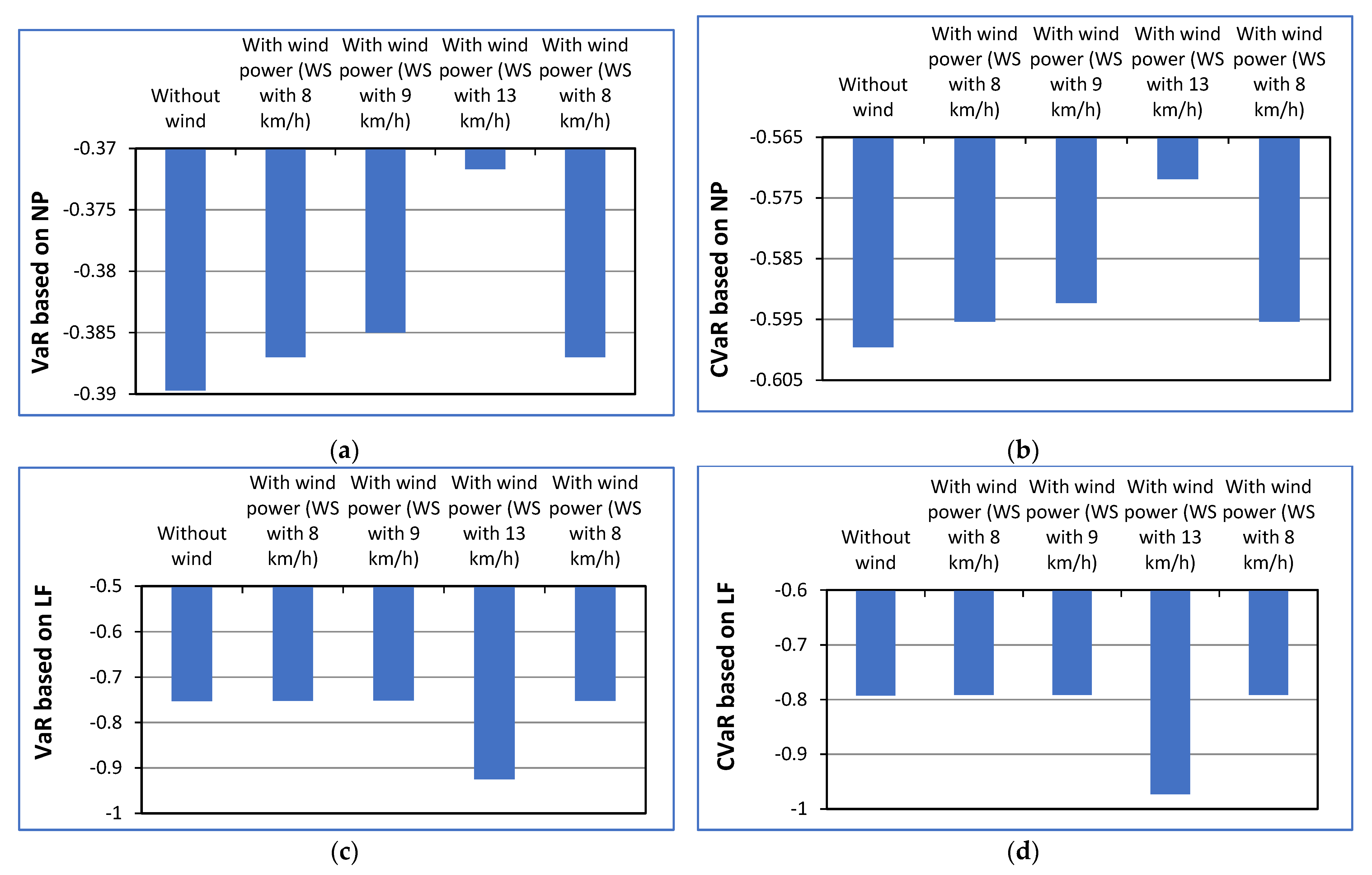
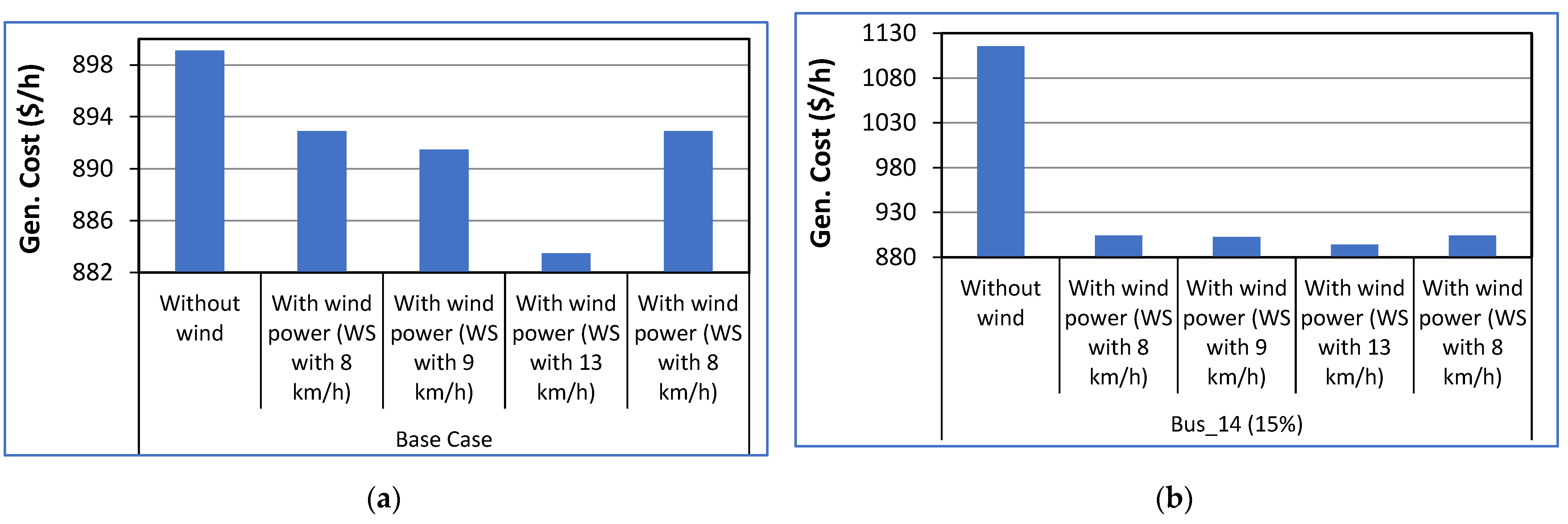
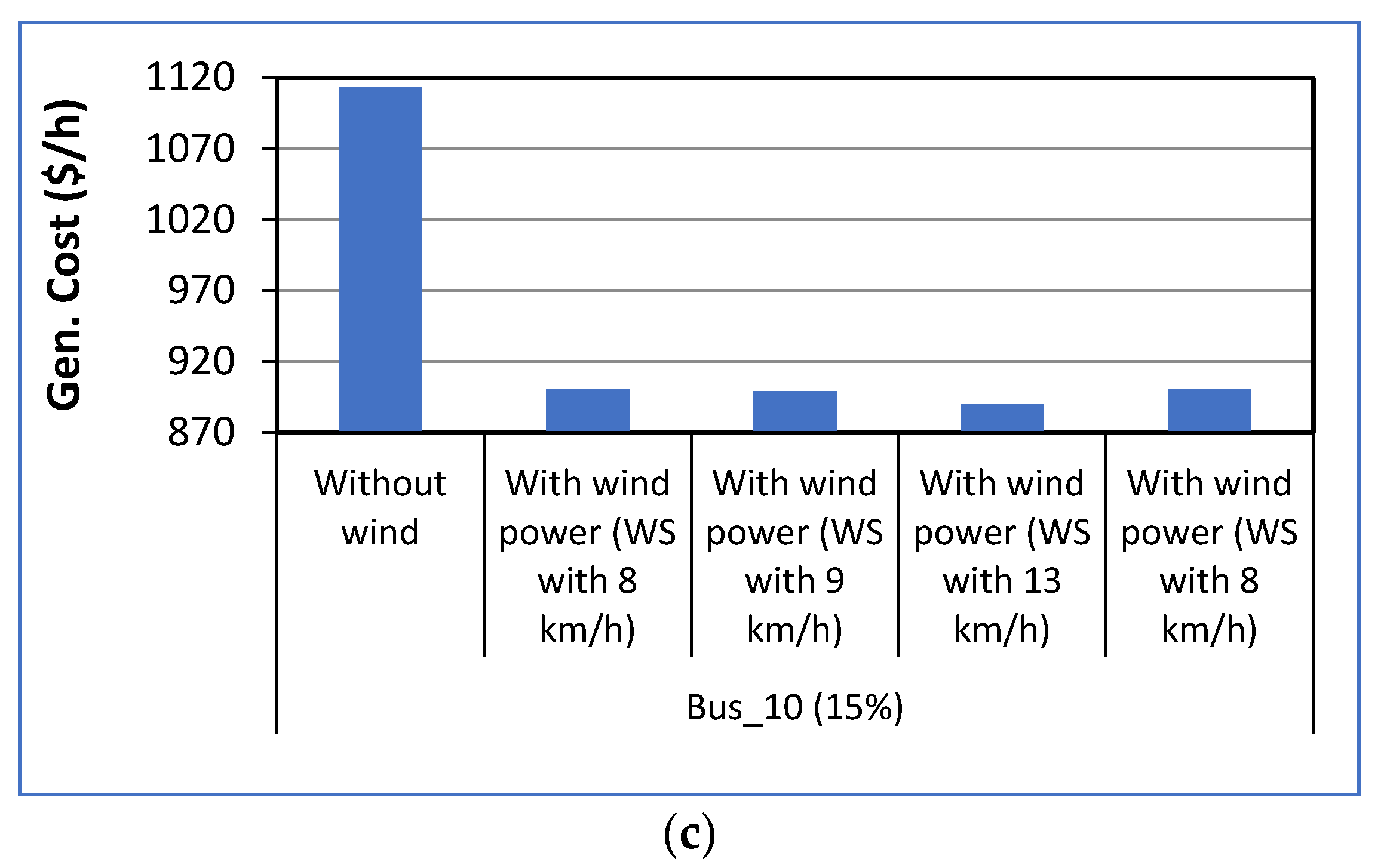
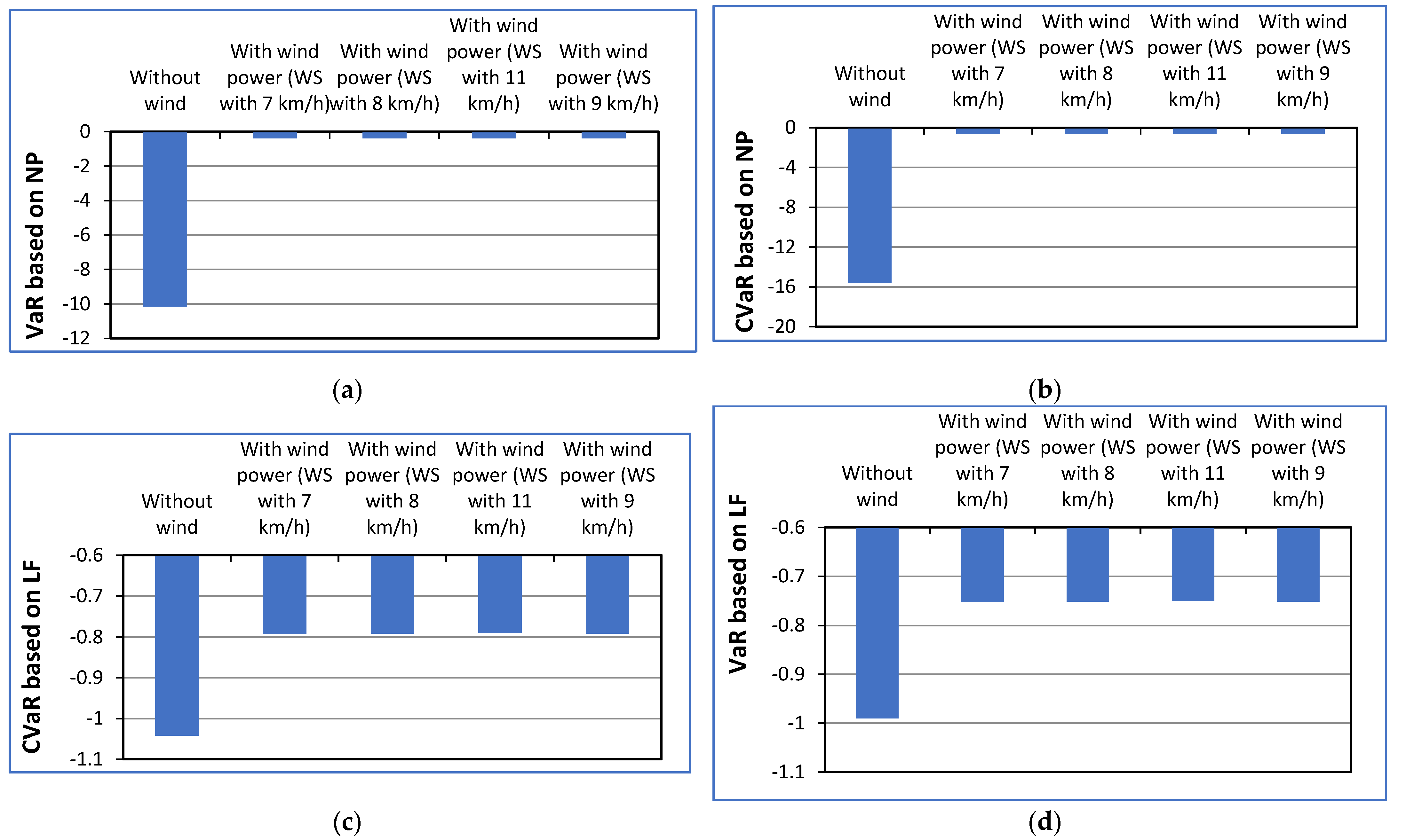
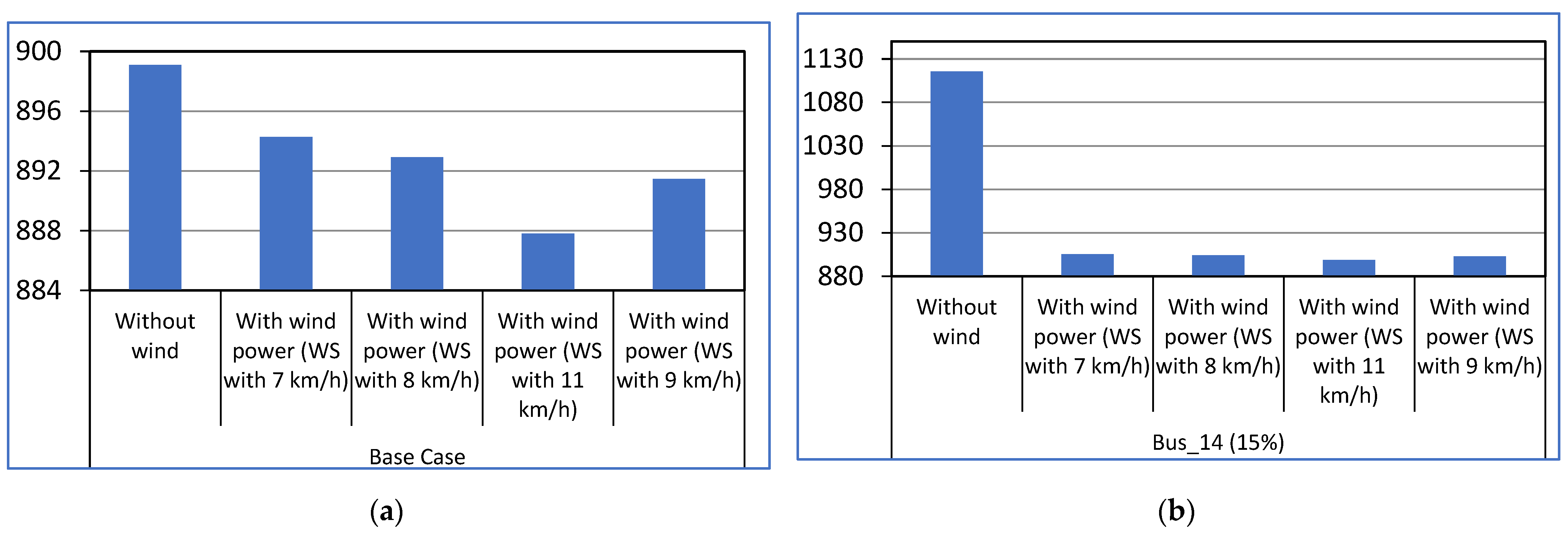
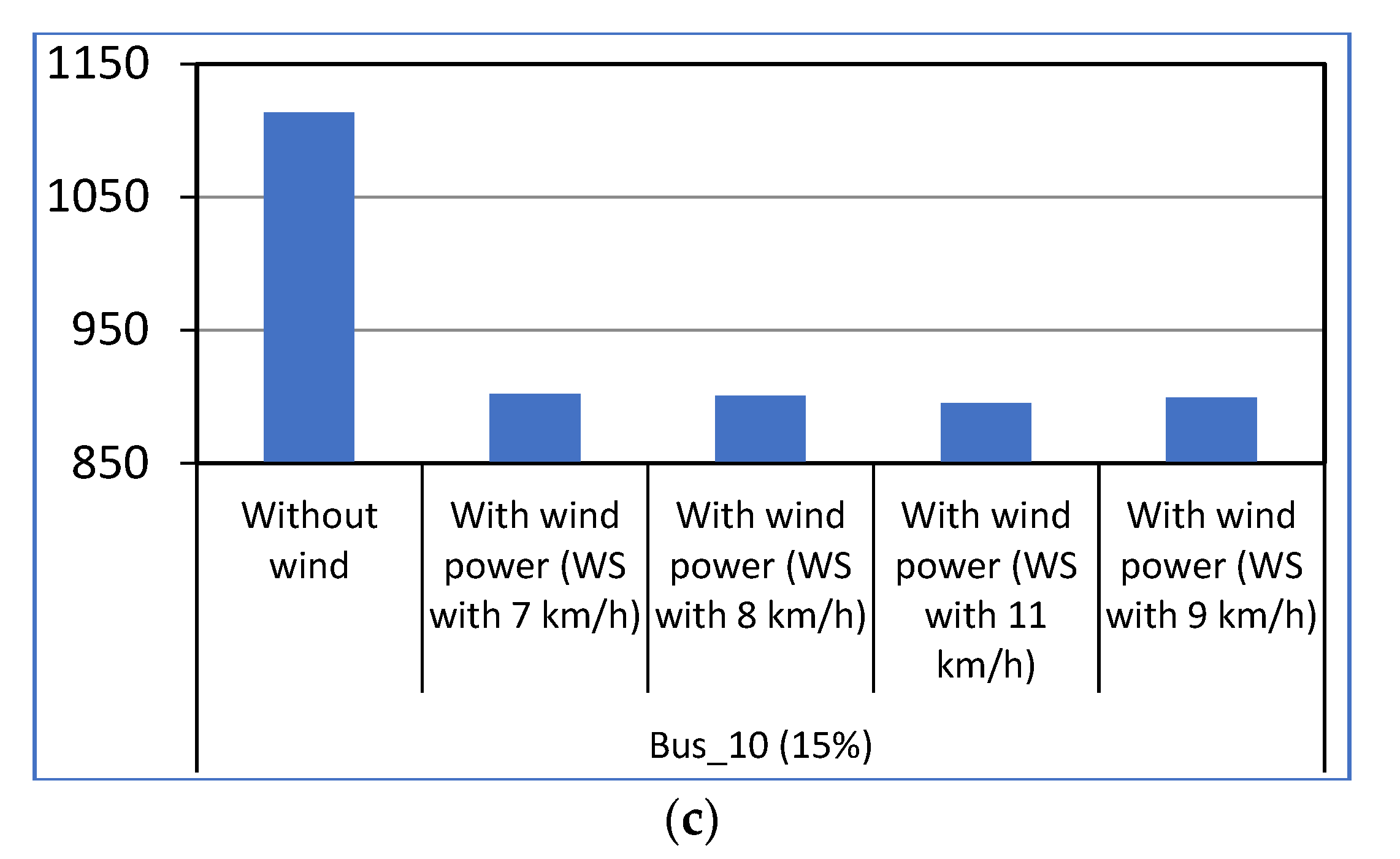
Wind power has also been considered in this work as the secondary source of generation beside the thermal power, which is working as the primary energy source.

Table 4. System Risk and Profit with Wind Power Integration (Kolhapur).

Sl. No.	Details	Wind Power (km/h)	Revenue ($/h)	Generation Cost ($/h)	Profit ($/h)	NP		LF
						VaR	CVaR	VaR	CVaR
1	Base Case_(0.0 h)	8	1212.317	892.902	319.415	−0.387	−0.5954	−0.752	−0.7915
2	Base Case_(6.0 h)	9	1208.188	891.468	316.72	−0.385	−0.5923	−0.7515	−0.7911
3	Base Case_(12.0 h)	13	1179.431	883.47	295.961	−0.3717	−0.5719	−0.9246	−0.9732
4	Base Case_(18.0 h)	8	1212.317	892.902	319.415	−0.387	−0.5954	−0.752	−0.7915
5	Bus_14 (15%)_(0.0 h)	8	1230.963	904.232	326.731	−0.3898	−0.5996	−0.7553	−0.7951
6	Bus_14 (15%)_(6.0 h)	9	1226.665	902.71	323.955	−0.3878	−0.5966	−0.755	−0.7947
7	Bus_14 (15%)_(12.0 h)	13	1196.225	894.14	302.085	−0.3746	−0.5763	−0.8833	−0.9298
8	Bus_14 (15%)_(18.0 h)	8	1230.963	904.232	326.731	−0.3898	−0.5996	−0.7553	−0.7951
9	Bus_10 (15%)_(0.0 h)	8	1226.94	900.482	326.458	−0.3903	−0.6005	−0.7521	−0.7917
10	Bus_10 (15%)_(6.0 h)	9	1222.536	898.931	323.605	−0.3883	−0.5974	−0.7517	−0.7913
11	Bus_10 (15%)_(12.0 h)	13	1191.6	890.13	301.47	−0.375	−0.577	−0.8823	−0.9287
12	Bus_10 (15%)_(18.0 h)	8	1226.94	900.482	326.458	−0.3903	−0.6005	−0.7521	−0.7917

displays the system risk, along with the risk assessment parameters, after the placement of the wind farm at bus no. 4 for Kolhapur. Figure 3 shows risk assessment parameter values, which have been calculated based on system NP and transmission line power flow (LF) for base cases of Kolhapur. The system generation costs with wind farms for different considered cases in Kolhapur is shown in Figure 4. From these results, it can be concluded that the highest values of wind farm placement reduce system risk and system generation costs in higher quantities. This happens due to the additional power supply to the grid by the wind farm.

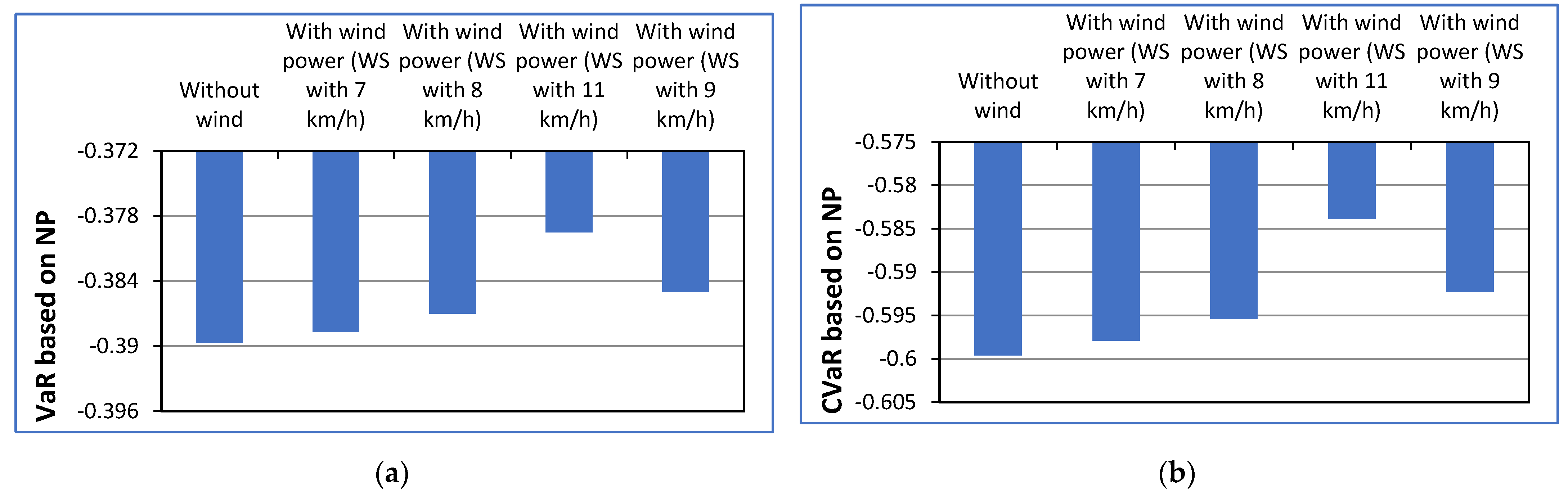
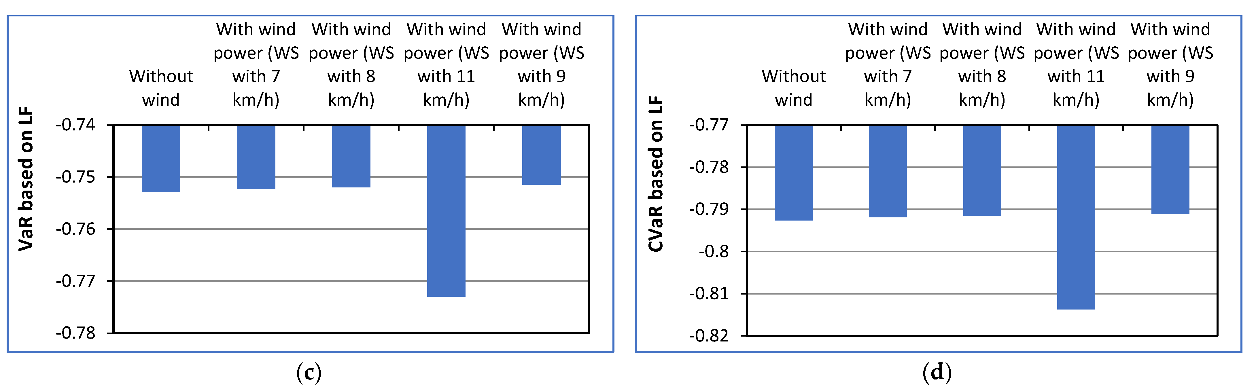
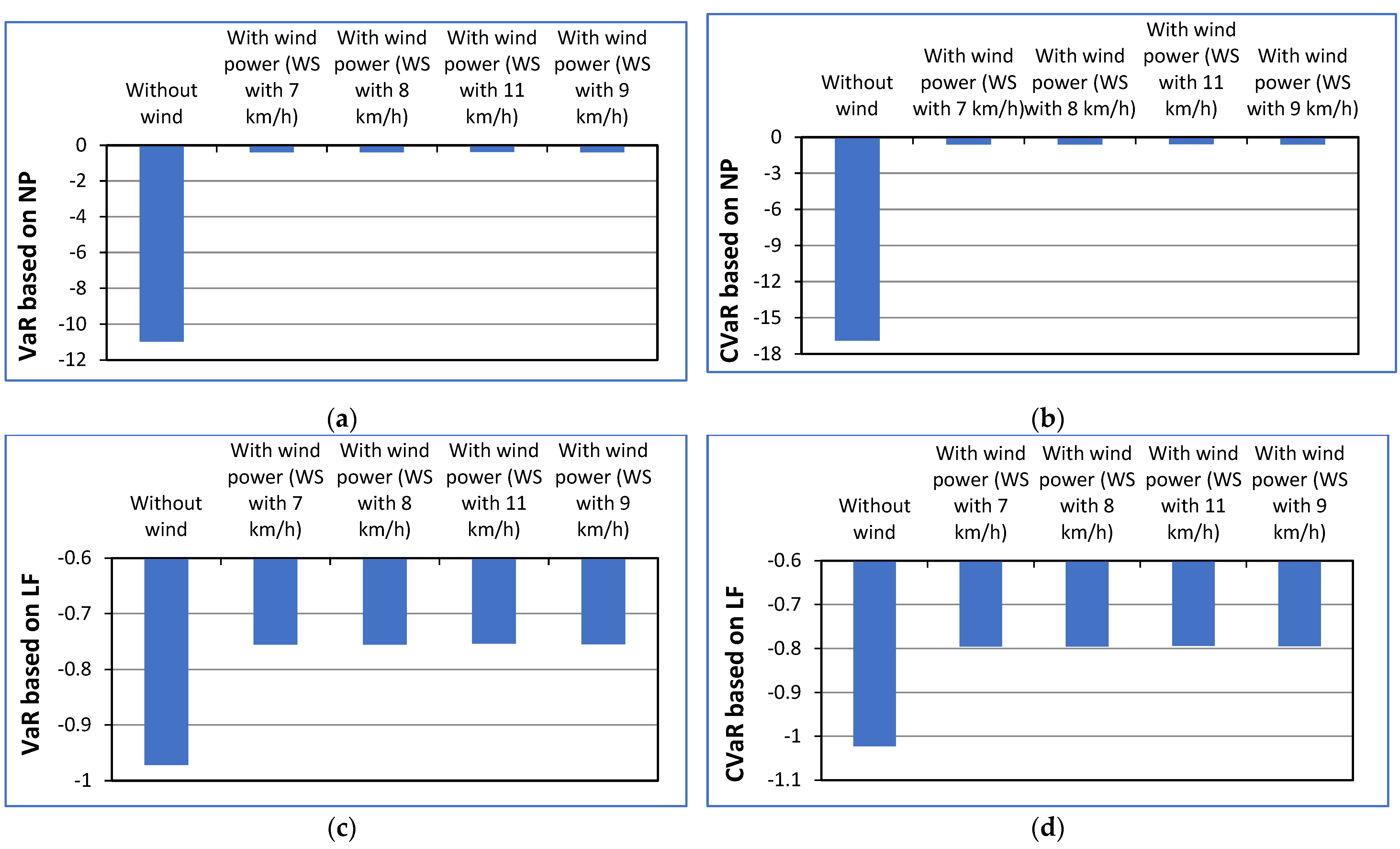
Similar to the previous case (i.e., Kolhapur), in this case (i.e., Mumbai), the impact of wind placement on the system risk has been obtained. The optimal location of a wind farm delivers extra protection to the electrical system by providing the additional power generated. The negative maximum values of VaR and CVaR deliver the minimum profit and maximum risk for the power system shown in Figure 1. It is necessary to shift the values of VaR and CVaR toward the right-hand side to deliver maximum profit. Figure 5, Figure 6 and Figure 7 show the VaR and CVaR values after placement of the wind farm in modified IEEE 14-bus systems for Mumbai. Four different amounts of wind power are merged into the system to show the variable nature of wind power. From the results, it is understood that after the placement of maximum quantities of wind farms in the system, the system risk is minimized. The same scenario is also observed for system generation costs. The maximum quantities of wind power provide a minimum generation cost-based system. These results directly support the incorporation of wind farms with high capacity in a deregulated power system to mitigate system risks and maximize system profit.

The comparative studies of system generation cost with and without placement of wind farms for the IEEE 14-bus system considering the cases of Mumbai are shown in Figure 8. It can be seen that the generation cost is reduced by a huge amount after the placement of the highest values of wind power in the system. Therefore, it can be concluded that the placement of WF provides risk minimization and generation cost minimization for any power system.

• Case 3: With Wind Placement and Considering Imbalance Cost (Modified IEEE 14-bus System)

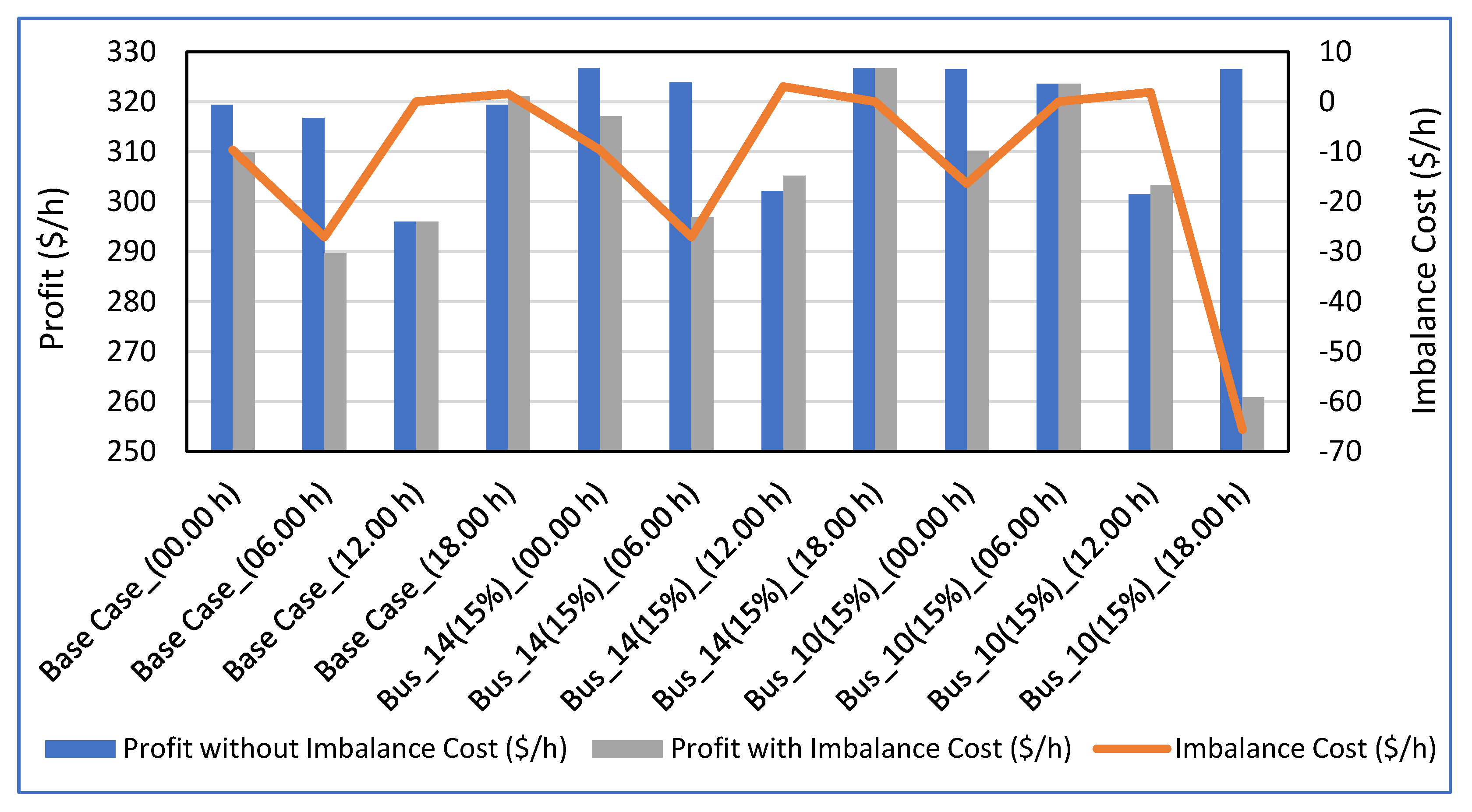
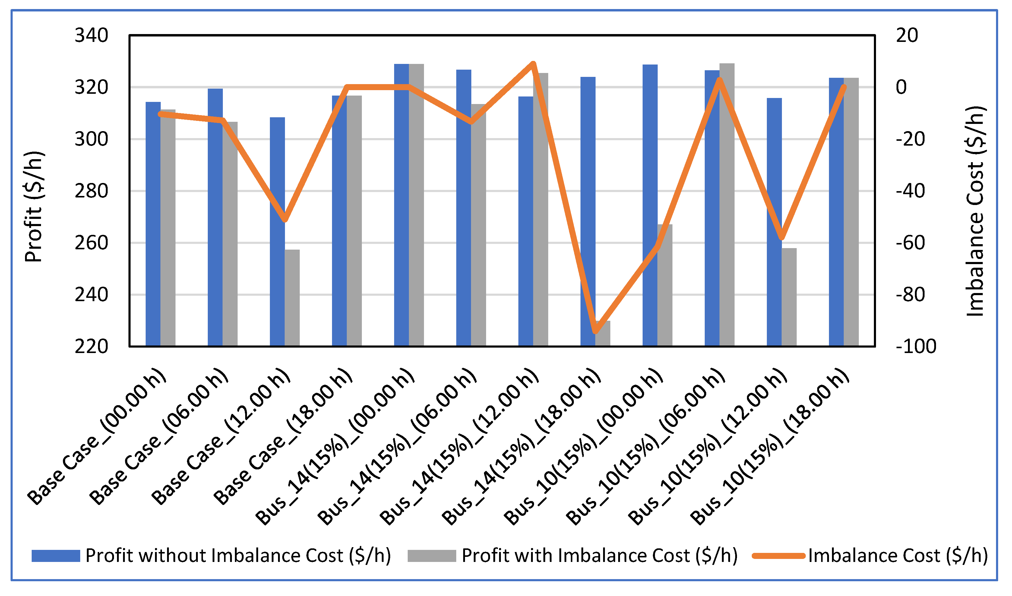
In the deregulated system, wind farms need to submit the future power generation scenario to the ISO before the date of operation. Based on their submitted data of power, ISO scheduled power generation from different generating stations. In reality, the wind farm cannot generate the scheduled power in maximum cases due to the uncertain nature of the wind flow. The violation of market contracts can impose an economic burden (i.e., imbalance cost) on the generating companies. The imbalance cost directly affects the system economy. When RWP is more than the EWP, then ISO gives rewards to the wind farm for their surplus power supply; however, ISO imposes a penalty if EWP is more than RWP. Thus, the adverse effect of imbalance costs directly disturbs the economic advancement of the market players. Here, the imbalance cost is calculated for every considered variation in expected and real wind speeds. The imbalance cost of the system reflects the mismatch between the predicted and real wind speed data. The imbalance cost is maximum when the difference between expected and real wind speed is maximum. When the expected wind speed is large compared to the real wind speed, the deficit charge rate arises, and when the real wind speed is larger than the expected wind speed, the surplus charge rate occurs. The deficit and surplus charge rates are zero for that case when the expected and real wind speeds are the same. Using the deficit and surplus charge rates, the total imbalance cost of the electrical system can be calculated. The imbalance cost is ‘−ve’ when ISO imposes the penalty on the generating station for their deficit supply of power from renewable sources. However, the imbalance cost is ‘+ve’ when ISO provides the reward to the generating station for their surplus supply of power from renewable energy sources. Here, the imbalance cost is calculated for every variation in the expected and real wind speeds using the formula stated in Equations (13)–(16). Both expected and real wind speed data have been taken for Kolhapur and Mumbai, Maharashtra to check the effectiveness of the proposed method.

Table 5. Profit Comparison with Imbalance Cost (Kolhapur).

Sl. No.	Details	Generation Cost ($/h)	Revenue ($/h)	Profit without Imbalance Cost ($/h)	Real Wind Power (km/h)	Expected Wind Power (km/h)	Imbalance Cost ($/h)	Profit with Imbalance Cost ($/h)
1	Base Case_(00.00 h)	892.902	1212.317	319.415	8	9	−9.601	309.814
2	Base Case_(06.00 h)	891.468	1208.188	316.72	9	11	−27.07	289.65
3	Base Case_(12.00 h)	883.47	1179.431	295.961	13	13	0	295.961
4	Base Case_(18.00 h)	892.902	1212.317	319.415	8	7	1.602	321.017
5	Bus_14(15%)_(00.00 h)	904.232	1230.963	326.731	8	9	−9.6017	317.1293
6	Bus_14(15%)_(06.00 h)	902.71	1226.665	323.955	9	11	−27.0724	296.8826
7	Bus_14(15%)_(12.00 h)	894.14	1196.225	302.085	13	7	3.0779	305.1629
8	Bus_14(15%)_(18.00 h)	904.232	1230.963	326.731	8	8	0	326.731
9	Bus_10(15%)_(00.00 h)	900.482	1226.94	326.458	8	9	−16.3831	310.0749
10	Bus_10(15%)_(06.00 h)	898.931	1222.536	323.605	9	9	0	323.605
11	Bus_10(15%)_(12.00 h)	890.13	1191.6	301.47	13	11	1.8957	303.3657
12	Bus_10(15%)_(18.00 h)	900.482	1226.94	326.458	8	11	−65.58	260.878

and

Table 6. Profit Comparison with Considering Imbalance Cost (Mumbai).

Sl. No.	Details	Generation Cost ($/h)	Revenue ($/h)	Profit without Imbalance Cost ($/h)	Real Wind Power (km/h)	Expected Wind Power (km/h)	Imbalance Cost ($/h)	Profit with Imbalance Cost ($/h)
1	Base Case_(00.00 h)	894.28	1216.005	314.295	7	8	−10.43	311.295
2	Base Case_(06.00 h)	892.902	1212.317	319.415	8	9	−12.89	306.525
3	Base Case_(12.00 h)	887.8	1196.124	308.324	11	13	−51.03	257.294
4	Base Case_(18.00 h)	891.468	1208.188	316.72	9	9	0	316.72
5	Bus_14(15%)_(00.00 h)	905.42	1234.303	328.883	7	7	0	328.883
6	Bus_14(15%)_(06.00 h)	904.232	1230.963	326.731	8	9	−13.33	313.401
7	Bus_14(15%)_(12.00 h)	898.83	1215.162	316.332	11	8	9.0246	325.3566
8	Bus_14(15%)_(18.00 h)	902.718	1226.655	323.937	9	13	−94.0949	229.8421
9	Bus_10(15%)_(00.00 h)	901.71	1230.382	328.672	7	11	−61.5737	267.0983
10	Bus_10(15%)_(06.00 h)	900.48	1226.94	326.46	8	7	2.6938	329.1538
11	Bus_10(15%)_(12.00 h)	894.98	1210.795	315.815	11	13	−57.936	257.879
12	Bus_10(15%)_(18.00 h)	898.93	1222.536	323.606	9	9	0	323.606

depict the profit comparison considering the imbalance costs for Kolhapur and Mumbai, respectively.

The impact of imbalance cost on system profit has shown in Figure 9 and Figure 10 for Kolhapur and Mumbai respectively. In the last considered case, the real wind speed is 8 km/h whereas the expected wind speed was 11 km/h. This is the maximum amount of mismatch in wind speed. Therefore, at this hour, the impact of imbalance cost is also high.

• Case 4: Solar PV-Battery Operation with SQP, ABC, and AGTO (Modified IEEE 14-bus System)

After a detailed study of the first 3 cases, it is found that the system imbalance cost is very dangerous for the economic operation of generating stations. If the imbalance cost is positive, the profit of the generation unit increases, but the system profit is lower for the negative imbalance cost. In this scenario, solar PV and battery hybrid systems play a vital role in mitigating the mismatch between real and expected wind power and minimizing dependency on the thermal power plant. Environmental benefits can also be obtained by using a solar PV-battery system. To check the effectiveness of the presented method, three different optimization techniques have been used.

The solar PV-battery storage system has been placed on bus no. 9 with a supply capacity of 2 MW. Here, the modeling of solar PV-battery storage systems has not been considered. Only a fixed value of generated power from a solar PV-battery storage system has been chosen. The placement bus has been considered at 9 due to the large load connected to that particular bus.

Table 7. System profit with different optimization techniques.

Sl. No.	Details	Kolhapur				Mumbai
		Profit with Imbalance Cost ($/h) Using SQP without Solar PV-Battery	Profit with Imbalance Cost ($/h) Using SQP with Solar PV-Battery	Profit with Imbalance Cost ($/h) Using ABC with Solar PV-Battery	Profit with Imbalance Cost ($/h) Using AGTO with Solar PV-Battery	Profit with Imbalance Cost ($/h) Using SQP without Solar PV-Battery	Profit with Imbalance Cost ($/h) Using SQP with Solar PV-Battery	Profit with Imbalance Cost ($/h) Using ABC with Solar PV-Battery	Profit with Imbalance Cost ($/h) Using AGTO with Solar PV-Battery
1	Base Case_(00.00 h)	309.814	313.265	318.256	319.165	311.295	315.354	320.651	321.425
2	Base Case_(06.00 h)	289.65	293.698	299.032	300.168	306.525	310.265	315.321	316.521
3	Base Case_(12.00 h)	295.961	299.021	304.658	305.785	257.294	261.954	266.357	267.462
4	Base Case_(18.00 h)	321.017	325.964	330.254	331.457	316.72	320.547	325.835	327.125
5	Bus_14(15%)_(00.00 h)	317.1293	321.238	326.265	327.158	328.883	332.154	337.254	338.652
6	Bus_14(15%)_(06.00 h)	296.8826	300.982	305.954	307.054	313.401	317.561	322.647	323.851
7	Bus_14(15%)_(12.00 h)	305.1629	309.347	314.325	315.647	325.3566	329.617	334.247	335.324
8	Bus_14(15%)_(18.00 h)	326.731	330.657	335.931	337.265	229.8421	233.991	238.487	239.623
9	Bus_10(15%)_(00.00 h)	310.0749	314.0535	320.654	321.781	267.0983	271.364	276.954	278.126
10	Bus_10(15%)_(06.00 h)	323.605	327.835	333.254	334.438	329.1538	333.614	338.725	339.957
11	Bus_10(15%)_(12.00 h)	303.3657	307.215	312.657	313.981	257.879	261.983	266.587	267.754
12	Bus_10(15%)_(18.00 h)	260.878	264.325	270.258	271.435	323.606	327.751	332.652	333.723

and

Table 8. System risk with different optimization techniques (for Kolhapur).

Sl. No.	Details	NP
		VaR				CVaR
		With Wind Farm Using SQP	With Wind Farm-Solar PV-Battery Storage Using SQP	With Wind Farm-Solar PV-Battery Storage Using ABC	With Wind Farm-Solar PV-Battery Storage Using AGTO	With Wind Farm Using SQP	With Wind Farm-Solar PV-Battery Storage Using SQP	With Wind Farm-Solar PV-Battery Storage Using ABC	With Wind Farm-Solar PV-Battery Storage Using AGTO
1	Base Case_(12.0 h)	−0.3717	−0.3615	−0.3525	−0.3419	−0.5719	−0.5526	−0.5416	−0.5316
2	Bus_14 (15%)_(12.0 h)	−0.3746	−0.3634	−0.3548	−0.3439	−0.5763	−0.5586	−0.5474	−0.5357
3	Bus_10 (15%)_(12.0 h)	−0.375	−0.3647	−0.3559	−0.3442	−0.577	−0.5591	−0.5465	−0.5368

show the comparative studies of system profit and system risk with different optimization techniques. For risk assessment studies, some selected cases have been considered for Kolhapur. From both tables, it is observed that AGTO techniques provide the best results among all considered cases by providing accurate optimal settings to minimize the system risk and maximize the system profit. Therefore, it can be concluded that the solar PV-battery storage system can reduce the negative impact of imbalance costs in the system economy and minimize system risk.

• Case 5: Solar PV-Battery Operation with SQP, ABC, and AGTO for Kolhapur (Modified IEEE 30-bus system)

Similar to the modified IEEE 14-bus system, the impact assessment of solar PV and battery storage systems has also been investigated for the modified IEEE 30-bus system. The system data has been taken from [33]. Only the base case of Kolhapur with four time intervals (i.e., 0.0 h, 6.0 h, 12.0 h, and 18.0 h) has been studied for the modified IEEE 30-bus system. The same wind speeds have been considered here as the 14-bus system. A combined amount of 2 MW of power from a solar PV-battery storage system has been chosen.

Table 9. System profit with different optimization techniques (for Kolhapur).

Sl. No.	Details	Kolhapur
		Profit with Imbalance Cost ($/h) Using SQP without Solar PV-Battery	Profit with Imbalance Cost ($/h) Using SQP with Solar PV-Battery	Profit with Imbalance Cost ($/h) Using ABC with Solar PV-Battery	Profit with Imbalance Cost ($/h) Using AGTO with Solar PV-Battery
1	Base Case_(00.00 h)	324.268	329.658	335.627	336.751
2	Base Case_(06.00 h)	297.685	302.685	308.776	310.021
3	Base Case_(12.00 h)	307.247	312.654	318.168	319.685
4	Base Case_(18.00 h)	341.038	346.658	352.951	354.237

and

Table 10. System risk with different optimization techniques (for Kolhapur).

Sl. No.	Details	NP
		VaR				CVaR
		With Wind Farm Using SQP	With Wind Farm-Solar PV-Battery Storage Using SQP	With Wind Farm-Solar PV-Battery Storage Using ABC	With Wind Farm-Solar PV-Battery Storage Using AGTO	With Wind Farm Using SQP	With Wind Farm-Solar PV-Battery Storage Using SQP	With Wind Farm-Solar PV-Battery Storage Using ABC	With Wind Farm-Solar PV-Battery Storage Using AGTO
1	Base Case_(12.0 h)	−0.3735	−0.3667	−0.3521	−0.3434	−0.5753	−0.5567	−0.5423	−0.5334
2	Bus_14 (15%)_(12.0 h)	−0.3748	−0.3675	−0.3536	−0.3445	−0.5771	−0.5574	−0.5446	−0.5348
3	Bus_10 (15%)_(12.0 h)	−0.3759	−0.3686	−0.3571	−0.3462	−0.5792	−0.5585	−0.5475	−0.5359

show comparative studies of system profit and system risk with different optimization techniques. For risk assessment studies, base cases have been considered for Kolhapur. From both tables, it is observed that AGTO techniques offer the finest results among all considered cases by providing accurate optimal settings. Therefore, it can be concluded that the solar PV-battery storage system can also reduce the negative impact of imbalance costs in the modified IEEE 30-bus system in terms of profit maximization. The system risk has also been minimized after the placement of solar PV and battery storage systems.

6. Conclusions

The hybrid effect of solar PV, wind farms, and battery storage systems on power system economics has been considered in this paper. To authenticate the task, a deregulated power market was considered. To evaluate system risk, Value-at-risk (VaR) and Cumulative Value-at-risk (CVaR) have been used here. The stability and safety of an electrical system can be improved by minimizing system risk. The placement of solar PV and battery storage systems minimizes the negative impact of system imbalance costs, which are developed due to the disparity between the bidding and running wind power quantities. The hybrid system minimizes system risk, which can further reduce the instability conditions of the system. To examine the effect of system risk considering wind farms with solar PV-battery storage systems under deregulated power systems, comparative studies are conducted using different optimization techniques, such as the Artificial Gorilla Troops Optimizer Algorithm (AGTO), Artificial Bee Colony Algorithms (ABC), and Sequential Quadratic Programming (SQP). The modified IEEE 14-bus and modified IEEE 30-bus systems have been used here to analyze the efficiency and robustness of the presented work. As evident from the results, the presence of a solar PV-battery storage system with a wind farm improves the economic parameters of the system by reducing the system risk. The Artificial Gorilla Troops Optimizer Algorithm (AGTO) has been used for the first time in this kind of risk mitigation problem, which is the uniqueness of this paper. This work can be performed with different renewable energy sources and energy storage devices in the near future for any small or large electrical system.

References

- Ustun, T.S.; Aoto, Y. Analysis of Smart Inverter’s Impact on the Distribution Network Operation. IEEE Access 2019, 7, 9790–9804. [Google Scholar]
- Farooq, Z.; Rahman, A.; Hussain, S.S.; Ustun, T.S. Power Generation Control of Renewable Energy Based Hybrid Deregulated Power System. Energies 2022, 15, 517. [Google Scholar]
- Public Utility Regulatory Policies Act of 1978 (PURPA), Office of Electricity, U.S. Department of Energy. Available online: https://www.energy.gov/oe/services/electricity-policy-coordination-and-implementation/other-regulatory-efforts/public (accessed on 1 March 2022).
- Latif, A.; Paul, M.; Das, D.C.; Hussain, S.S.; Ustun, T.S. Price Based Demand Response for Optimal Frequency Stabilization in ORC Solar Thermal Based Isolated Hybrid Microgrid under Salp Swarm Technique. Electronics 2020, 9, 2209. [Google Scholar]
- Ustun, T.S.; Aoto, Y.; Hashimoto, J.; Otani, K. Optimal PV-INV Capacity Ratio for Residential Smart Inverters Operating Under Different Control Modes. IEEE Access 2020, 8, 116078–116089. [Google Scholar]
- Hussain, S.S.; Nadeem, F.; Aftab, M.A.; Ali, I.; Ustun, T.S. The Emerging Energy Internet: Architecture, Benefits, Challenges, and Future Prospects. Electronics 2019, 8, 1037. [Google Scholar]
- GM Abdolrasol, M.; Hannan, M.A.; Hussain, S.S.; Ustun, T.S.; Sarker, M.R.; Ker, P.J. Energy Management Scheduling for Microgrids in the Virtual Power Plant System Using Artificial Neural Networks. Energies 2021, 14, 6507. [Google Scholar]
- Ustun, T.S.; Ozansoy, C.; Zayegh, A. Extending IEC 61850-7-420 for distributed generators with fault current limiters. In Proceedings of the 2011 IEEE PES Innovative Smart Grid Technologies, Perth, Australia, 13–16 November 2011; pp. 1–8. [Google Scholar]
- Kumar, K.K.P.; Soren, N.; Latif, A.; Das, D.C.; Hussain, S.S.; Al-Durra, A.; Ustun, T.S. Day-Ahead DSM-Integrated Hybrid-Power-Management-Incorporated CEED of Solar Thermal/Wind/Wave/BESS System Using HFPSO. Sustainability 2022, 14, 1169. [Google Scholar]
- Arango-Aramburo, S.; Bernal-García, S.; Larsen, E.R. Renewable energy sources and the cycles in deregulated electricity markets. Energy 2021, 223, 120058. [Google Scholar]
- Yao, X.; Yi, B.; Yu, Y.; Fan, Y.; Zhu, L. Economic analysis of grid integration of variable solar and wind power with conventional power system. Appl. Energy 2020, 264, 114706. [Google Scholar]
- Ustun, T.S.; Nakamura, Y.; Hashimoto, J.; Otani, K. Performance analysis of PV panels based on different technologies after two years of outdoor exposure in Fukushima, Japan. Renew. Energy 2019, 136, 159–178. [Google Scholar]
- Hou, S.; Yi, B.W.; Zhu, X. Potential economic value of integrating concentrating solar power into power grids. Comput. Ind. Eng. 2021, 160, 107554. [Google Scholar]
- Kumar, A.; Bag, B. Incorporation of probabilistic solar irradiance and normally distributed load for the assessment of ATC. In Proceedings of the 2017 8th International Conference on Computing, Communication and Networking Technologies (ICCCNT) IEEE Transactions on Power Systems, Delhi, India, 3–5 July 2017; Volume 13, pp. 1–6. [Google Scholar]
- Reddy, S.S. Optimal scheduling of thermal-wind-solar power system with storage. Renew. Energy 2017, 101, 1357–1368. [Google Scholar]
- Nadeem, F.; Aftab, M.A.; Hussain, S.S.; Ali, I.; Tiwari, P.K.; Goswami, A.K.; Ustun, T.S. Virtual Power Plant Management in Smart Grids with XMPP Based IEC 61850 Communication. Energies 2019, 12, 2398. [Google Scholar]
- Reddy, S.S.; Bijwe, P.R. Day-Ahead and Real Time Optimal Power Flow considering Renewable Energy Resources. Electr. Power Energy Syst. 2016, 82, 400–408. [Google Scholar]
- Gope, S.; Goswami, A.K.; Tiwari, P.K. Transmission congestion management using a wind integrated compressed air energy storage system. Eng. Technol. Appl. Sci. Res. 2017, 7, 1746–1752. [Google Scholar]
- Xu, X.; Ye, Z.; Qian, Q. Economic, exergoeconomic analyses of a novel compressed air energy storage-based cogeneration. J. Energy Storage 2022, 51, 104333. [Google Scholar] [CrossRef]
- Sun, S.; Kazemi-Razi, S.M.; Kaigutha, L.G.; Marzband, M.; Nafisi, H.; Al-Sumaiti, A.S. Day-ahead offering strategy in the market for concentrating solar power considering thermoelectric decoupling by a compressed air energy storage. Appl. Energy 2022, 305, 117804. [Google Scholar] [CrossRef]
- Chang, Y.C.; Lee, T.Y.; Chen, C.L.; Jan, R.M. Optimal power flow of a wind-thermal generation system. Electr. Power Energy Syst. 2014, 55, 312–320. [Google Scholar]
- Xu, Z.; Hu, Z.; Song, Y.; Wang, J. Risk-Averse Optimal Bidding Strategy for Demand-Side Resource Aggregators in Day-Ahead Electricity Markets Under Uncertainty. IEEE Trans. Smart Grid 2017, 8, 96–105. [Google Scholar]
- Matevosyan, J.; Soder, L. Minimization of Imbalance Cost Trading Wind Power on the Short-Term Power Market. IEEE Trans. Power Syst. 2016, 21, 1396–1404. [Google Scholar]
- Dawn, S.; Tiwari, P.K.; Goswami, A.K. An approach for efficient assessment of the performance of double auction competitive power market under variable imbalance cost due to high uncertain wind penetration. Renew. Energy 2017, 108, 230–248. [Google Scholar]
- Wu, J.; Zhang, B.; Jiang, Y.; Bie, P.; Li, H. Chance-constrained stochastic congestion management of power systems considering uncertainty of wind power and demand side response. Electr. Power Energy Syst. 2019, 107, 703–714. [Google Scholar]
- Rubin, O.D.; Babcock, B.A. The impact of expansion of wind power capacity and pricing methods on the efficiency of deregulated electricity markets. Energy 2013, 59, 676–688. [Google Scholar]
- Das, A.; Dawn, S.; Gope, S.; Ustun, T.S. A Strategy for System Risk Mitigation Using FACTS Devices in a Wind Incorporated Competitive Power System. Sustainability 2022, 14, 8069. [Google Scholar] [CrossRef]
- Patil, G.S.; Mulla, A.; Ustun, T.S. Impact of Wind Farm Integration on LMP in Deregulated Energy Markets. Sustainability 2022, 14, 4354. [Google Scholar] [CrossRef]
- Khamees, A.K.; Abdelaziz, A.Y.; Eskaros, M.R.; El-Shahat, A.; Attia, M.A. Optimal Power Flow Solution of Wind-Integrated Power System Using Novel Metaheuristic Method. Energies 2021, 14, 6117. [Google Scholar] [CrossRef]
- Xu, Y.; Lang, Y.; Wen, B.; Yang, X. An Innovative Planning Method for the Optimal Capacity Allocation of a HybridWind–PV–Pumped Storage Power System. Energies 2019, 12, 2809. [Google Scholar] [CrossRef] [Green Version]
- Dawn, S.; Tiwari, P.K.; Goswami, A.K.; Panda, R. An Approach for System Risk Assessment and Mitigation by Optimal Operation of Wind Farm and FACTS Devices in a Centralized Competitive Power Market. IEEE Trans. Sustain. Energy 2018, 10, 1054–1065. [Google Scholar] [CrossRef]
- Singh, N.K.; Koley, C.; Gope, S.; Dawn, S.; Ustun, T.S. An Economic Risk Analysis in Wind and Pumped Hydro Energy Storage Integrated Power System Using Meta-Heuristic Algorithm. Sustainability 2013, 13, 13542. [Google Scholar] [CrossRef]
- Dawn, S.; Tiwari, P.K.; Goswami, A.K. An approach for long term economic operations of competitive power market by optimal combined scheduling of wind turbines and FACTS controllers. Energy 2019, 181, 709–723. [Google Scholar]
- Das, A.; Dawn, S.; Gope, S.; Ustun, T.S. A Risk Curtailment Strategy for Solar PV-Battery Integrated Competitive Power System. Electronics 2022, 11, 1251. [Google Scholar] [CrossRef]
- Abdolrasol, M.G.M.; Hussain, S.M.S.; Ustun, T.S.; Sarker, M.R.; Hannan, M.A.; Mohamed, R.; Ali, J.A.; Mekhilef, S.; Milad, A. Artificial Neural Networks Based Optimization Techniques: A Review. Electronics 2021, 10, 2689. [Google Scholar]
- Latif, A.; Hussain, S.S.; Das, D.C.; Ustun, T.S. Double stage controller optimization for load frequency stabilization in hybrid wind-ocean wave energy based maritime microgrid system. Appl. Energy 2021, 282, 116171. [Google Scholar]
- Latif, A.; Hussain, S.S.; Das, D.C.; Ustun, T.S. Optimum Synthesis of a BOA Optimized Novel Dual-Stage PI − (1 + ID) Controller for Frequency Response of a Microgrid. Energies 2020, 13, 3446. [Google Scholar]
- Singh, S.; Chauhan, P.; Aftab, M.A.; Ali, I.; Hussain, S.S.; Ustun, T.S. Cost Optimization of a Stand-Alone Hybrid Energy System with Fuel Cell and PV. Energies 2020, 13, 1295. [Google Scholar]
- Dey, P.P.; Das, D.C.; Latif, A.; Hussain, S.S.; Ustun, T.S. Active Power Management of Virtual Power Plant under Penetration of Central Receiver Solar Thermal-Wind Using Butterfly Optimization Technique. Sustainability 2020, 12, 6979. [Google Scholar]
- Chauhan, A.; Upadhyay, S.; Khan, M.T.; Hussain, S.S.; Ustun, T.S. Performance Investigation of a Solar Photovoltaic/Diesel Generator Based Hybrid System with Cycle Charging Strategy Using BBO Algorithm. Sustainabiliy 2021, 13, 8048. [Google Scholar]
- Hussain, I.; Das, D.C.; Sinha, N.; Latif, A.; Hussain, S.S.; Ustun, T.S. Performance Assessment of an Islanded Hybrid Power System with Different Storage Combinations Using an FPA-Tuned Two-Degree-of-Freedom (2DOF) Controller. Energies 2020, 13, 5610. [Google Scholar]
- Abdollahzadeh, B.; Gharehchopogh, F.S.; Mirjalili, S. Artificial gorilla troops optimizer: A new Nature-inspired Metaheuristic Algorithm for Global Optimization Problems. Int. J. Intell. Syst. 2021, 36, 5887–5958. [Google Scholar]
- Karaboga, D.; Basturk, B. Artificial Bee Colony (ABC) Optimization Algorithm for Solving Constrained Optimization Problems. In Proceedings of the 12th International Fuzzy Systems Association World Congress on Foundations of Fuzzy Logic and Soft Computing, Cancun, Mexico, 18–21 June 2007; Springer: Berlin/Heidelberg, Germany, 2007; Volume 4529, pp. 789–798. [Google Scholar]
- Database. World Temperatures & Weather around the World. Available online: www.timeanddate.com/weather/ (accessed on 29 May 2022).
Figure 1.
VaR and CVaR Representation.
Figure 2.
Relation between generation cost and risk assessment tools. VaR based on NP (a), CvaR basd on NP (b), VaR based on LF (c), CvaR based on LF (d).
Figure 3.
System Risk with Wind Power Integration (Vijayawada @Base Case). VaR based on NP (a), CvaR basd on NP (b), VaR based on LF (c), CvaR based on LF (d).
Figure 4.
System Generation Costs ($/h) with Wind Power Integration (Kolhapur). Base case (a), Bus-14 15% (b), Bus_10 15% (c).
Figure 5.
System Risk with Wind Power Integration (Mumbai @Base Case). VaR based on NP (a), CvaR basd on NP (b), VaR based on LF (c), CvaR based on LF (d).
Figure 6.
System Risk with Wind Power Integration (Mumbai @ Bus_14 (15%)). VaR based on NP (a), CvaR basd on NP (b), VaR based on LF (c), CvaR based on LF (d).
Figure 7.
System Risk with Wind Power Integration (Mumbai @ Bus_10 (15%)). VaR based on NP (a), CvaR basd on NP (b), VaR based on LF (c), CvaR based on LF (d).
Figure 8.
System Generation Cost ($/h) with Wind Power Integration (Mumbai). Base case (a), Bus-14 15% (b), Bus_10 15% (c).
Figure 9.
Profit Comparison with Imbalance Cost (Kolhapur).
Figure 10.
Profit Comparison with Imbalance Cost (Mumbai).