
Thermal Network Model for an Assessment of Summer Indoor Comfort in a Naturally Ventilated Residential Building


Department of Power Systems and Environmental Protection Facilities, Faculty of Mechanical Engineering and Robotics, AGH University of Science and Technology, Mickiewicza 30, 30-059 Kraków, Poland
Energies 2022, 15(10), 3709; https://doi.org/10.3390/en15103709
Submission received: 31 March 2022
/
Revised: 9 May 2022
/
Accepted: 17 May 2022
/
Published: 18 May 2022
Abstract
:Costs of cooling installations cause them to be very rarely used in residential buildings in countries located in heating-dominated climates, like Poland. Hence, there arises the need to assess indoor thermal comfort during summer and to indicate ways to reduce possible overheating. This paper presents an attempt to use the thermal network model of the building zone of EN ISO 13790 to assess indoor operative temperature during four warm months from June to September. The model of the naturally ventilated single-family residential building located in central Poland was used. Performed calculations for the base case resulted in 38 and 63 days within the comfort zone at 80% acceptance level in a total of 122 days in the analyzed period for EN 15251 and ASHRAE standards, respectively. Use of external shading on windows and the roof with lower solar absorptance resulted in 46 and 70 days with acceptable conditions, respectively. Further application of night ventilation resulted in the 38 and 63 days, respectively. From the considered solutions in Polish climate conditions, windows shading seems to be the most efficient solution when controlling indoor comfort in residential buildings with no cooling system. A comparison of hourly operative temperature from that model with the detailed simulation in EnergyPlus showed a strong correlation with R2 = 0.934.
1. Introduction
The Directive on Energy Performance of Buildings (EPBD) from 2008 set the base for energy performance standards in buildings in European countries. Under its provisions, there were applied minimum requirements of the energy performance of new and existing buildings and the certification of their energy performance was ensured.
To be able to implement the Directive, many supporting standards were required. For the calculation of the sensible energy use for space heating and cooling, EN ISO 13790 [1] was introduced. It covers three methods: a fully prescribed monthly quasi-steady-state calculation method (plus, as a special option, a seasonal method); a fully prescribed simple hourly dynamic calculation method; and calculation procedures for detailed (e.g., hourly) dynamic simulation methods. They differ in complexity but equally can be used in energy certification, auditing and assessment of buildings. This wide field of application means that the research and development of these methods is important from a scientific and practical point of view.
From various types of building thermal models of buildings [2], the resistance-capacitance networks are of special interest. Based on thermal-electrical analogy they enable computation of transient heat flows within a zone simply and efficiently while maintaining ease of physical interpretation of network elements [3]. They also can be easily simplified through the lumping of elements and order-reduction [4]. However, as simplifications may result in non-negligible inaccuracies [5], validation studies are performed to check their quality.
The standard also allows using detailed simulation tools. In general, they are all based on a similar philosophy: the physical data of an object and its ambient environment must be entered and then results can be obtained. They offer a significantly wider range of calculation possibilities but require more detailed input data, professional knowledge, and time. For simpler applications where no sophisticated analyses are required to be performed, less demanding methods are likely to be used.
For these reasons for further considerations, the simple hourly method of EN ISO 13790 was chosen. It allows the introduction of hourly patterns for the building use and calculation of the cooling and heating loads in hourly time interval. A building zone is modelled here with the 5R1C resistance-capacitance thermal network model consisting of five thermal resistances and a single thermal capacitance lumping all partitions.
The simplicity and reasonable accuracy [6,7,8] of this model resulted in its popularity. Giving the base for further development [9] it was used in various applications as an assessment of energy consumption of buildings on a district scale [8,10], building integrated photovoltaic [11], double-skin facades [12], or varying ventilation airflow [13].
As noticed in [14], energy for space heating and cooling is supplied for the thermal comfort of people. Moreover, the 5R1C thermal model provides internal air and operative temperatures which can be potentially used for an evaluation of internal comfort [15]. For these reasons, it seems justified to study the usability of the model used in energy rating and certification of buildings for an assessment of indoor conditions in terms of thermal comfort. It can be especially important in residential buildings where no air conditioning operates and natural ventilation is used to estimate the possibility of overheating and study an impact of various measures to improve the quality of the indoor environment inside a considered object. Therefore, the following section presents works related to the aforementioned issues.
Powell et al. [16] investigated the Reflective Active Solar Facade (RASF) in terms of energy consumption reduction and indoor comfort improvement. The authors presented a calculation tool based on the 5R1C model to assess the hourly cooling and heating loads of a considered room. Solar gains were calculated from the Tonatiuh simulation ray-tracer coupled to the RC building model. Although authors stated that the presented RASF can improve occupancy comfort in a building, they neither performed comfort analysis nor gave indoor comfort indicators they considered.
In [17], the authors presented the developed simulation tool for an assessment of the whole energy, economic, environmental, and comfort performance of buildings with building-integrated solar thermal systems (BISTS). The thermal model of a building was based on a modified 5R1C scheme of EN ISO 13790. An additional module was also developed to estimate the Predicted Mean Vote (PMV). The whole procedure was implemented in Matlab. Finally, authors presented results of calculations of PMV for a single room in a multi-floor dwelling building.
Kalmár [18] used the 5R1C model to compute operative temperature in an educational building during summer conditions and then to obtain the PMV index. Results from measurements differed from calculated values in all cases because of the influence of direct solar irradiance on external walls and entering glazed rooms.
Shen et al. [19] modified the generic 5R1C model and introduced thermal coupling between zones into the computation algorithm. The developed building simulation program was written in Python. The tool was validated on the example of a 4-story educational building. The authors mentioned that it also computes PMV, but they didn’t present results related to the indoor comfort.
Csáky [20] presented experimental measurements of internal air and mean radiant temperature in two offices in Debrecen (Hungary). Based on these and the relevant meteorological data, the operative temperature and daily cooling energy demand were obtained using the RC thermal model of EN ISO 13790. Then, the thermal comfort in east and west-oriented rooms for different construction variants, including windows area, was assessed in the representative summer, hot, and torrid days using operative temperature calculated using the 5R1C model.
Oliveira Panão and Penas [21] investigated the generation of the building stock model and shift to transient energy calculations using the RC model from EN ISO 13790. The calculation procedure was implemented in Matlab and applied to the Lisbon Metropolitan Area. Authors focused on energy consumption in buildings, essential in Energy Performance Certification (EPC), required to maintain thermal comfort defined only by the indoor air temperature. Buildings without thermal comfort were determined as under-heated in winter or overheated in summer.
The 5R1C model is not a single case. As noticed in [22], thermal network models can be used to predict indoor comfort in buildings using PMV and PPD indicators. Taking advantage of this possibility, the authors showed the results of their research using various models.
The authors of [23] presented a complex resistance–capacitance model of the Building Integrated Photovoltaic Thermal solar collectors system (BIPV/T), written in Matlab [24]. The authors assessed the impact of the BIPV/T system on occupants’ comfort through PMV and PPD measures in a multi-floor office building in seven European locations. Other studies reflected on model predictive control (MPC) by applying higher order RC network models of buildings. This solution, however more detailed, resulted in complex mathematical description requiring the use of more sophisticated simulation tools, as Matlab [25,26].
Several conclusions can be drawn from the above overview. Despite its simplicity, the lumped capacitance model of a building zone of EN ISO 13790 offers good quality. It is intended for the calculation of sensible energy for space heating and cooling, first of all, in energy certification or auditing of buildings. That is probably the major reason why indoor comfort assessment using the 5R1C model was performed very rarely and as if by the way.
Presented analyses are based mainly on PMV and PPD indexes calculated from air temperature computed by the 5R1C model while assuming environmental conditions (as air velocity or clothing) following relevant standards requiring more complex tools. Only in one case indoor air temperature and in the second one operative temperature described indoor conditions. There were neither presented nor discussed possibilities of that model to be used in the evaluation of comfort together with energy performance simulation of a building. Moreover, only short-term considerations for selected days or periods of several days prevailed.
From the above, several objectives of the paper arise. The first is to select output variables from the R-C model of EN ISO 13790 to be used when describing indoor thermal comfort in a residential building. This will determine what range of analyses can be performed with it against the relevant international, especially European, standards. Then, the necessary simulations should be performed and the reliability of the obtained results should be verified regarding the professional building simulation tool. This way, the main question can be answered: to what extent the simple hourly method of EN ISO 13790, incorporating the 5R1C model, can be used in the evaluation of thermal comfort in residential buildings?
In the following section, the 5R1C model is presented along with the calculation procedure with emphasis on its outputs. Then, the American (ASHRAE 55) and European (EN 15251) standards related to indoor comfort in buildings are described in connection to the chosen simulation model. The next sections contain simulation assumptions, results, and discussion. After this, conclusions are given.
2. Materials and Methods
2.1. The 5R1C Model
The thermal network model of a building zone, given in the EN ISO 13790 standard, is intended for the calculation of sensible energy use for space heating and cooling in hourly time step. It can be used for several applications, such as comparing the energy performance of various cases at a design stage of a building, calculating of a standardized level of the energy performance of existing buildings, or assessing the effect of various possible energy conservation measures in an existing building on its energy use.
As mentioned above, the calculation procedures given in that standard is restricted to sensible heating and cooling. Hence, the energy use for humidification and dehumidification shall be calculated following the relevant standards. For these reasons, internal air humidity is not calculated here. It may be considered as an important disadvantage in terms of comfort analysis. However, as in residential buildings, air conditioning is rarely used and indoor humidity is a resultant variable this problem should be investigated in a separate study.
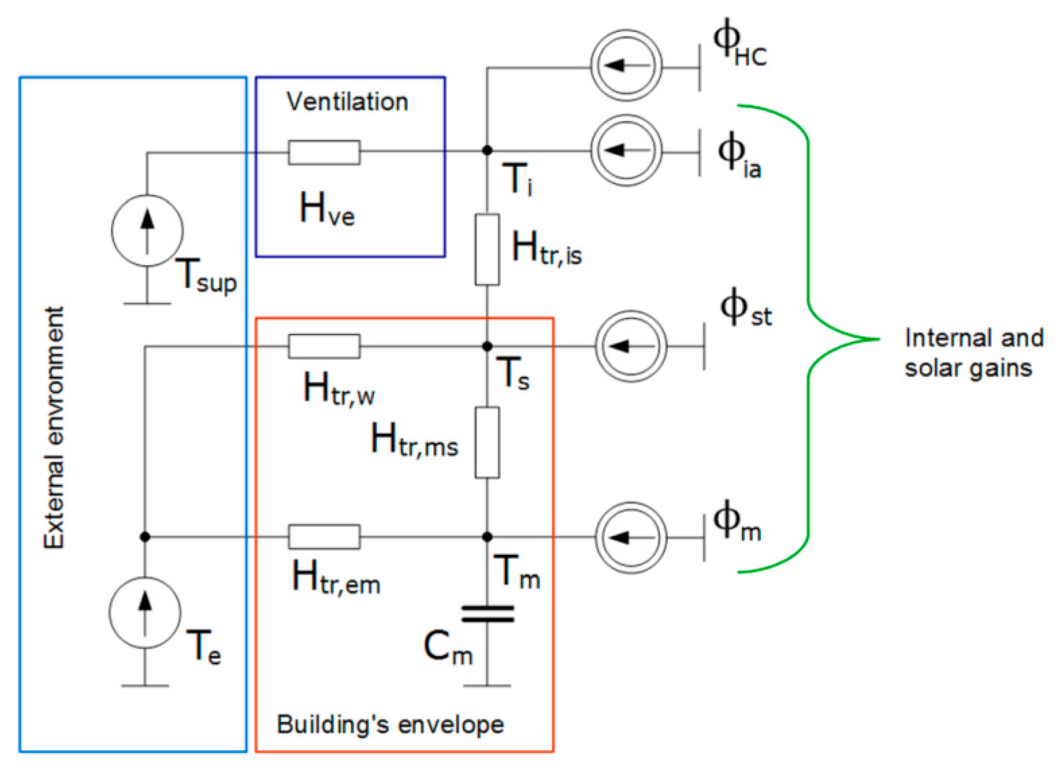
The 5R1C model consists of five thermal resistances and one capacitance (Figure 1).
Its physical interpretation has been given by several authors, recently [27,28,29,30,31]. Following them, the external partitions of negligible thermal mass (doors, windows, curtain walls, and glazed walls) are included in Htr,w thermal transmission coefficient. Thermally massive elements (walls or ceilings) are included in the Htr,op coefficient which is then divided into the external (Htr,em) and the internal (Htr,ms) parts connected the thermal capacity (Cm), which represents the thermal mass of the building. The external environment is represented by the ambient air temperature, Te, and supplying air temperature, Tsup, which is the temperature of ventilation air entering the building’s zone. The former acts on a building’s envelope. The latter is connected with the building’s interior through the heat transfer by ventilation (Hve).
The internal environment, important for indoor comfort analyses, is represented by two variables. The first one is the indoor air temperature, Ti, connected to ventilation heat transfer, heating and cooling source (φHC), and the coupling conductance (Htr,is). The second one is the central node temperature, Ts, which is a mix of indoor air temperature and mean radiant temperature (mean temperature of the internal surfaces).
Heat fluxes from internal sources (φint) and from solar radiation (φsol) are divided into φia, φst, and φm, connected to the indoor air node, the central node, and the thermal mass temperature node, respectively.
Thermal conductances and single capacitance can be obtained from the physical data of a building using the procedures given in that standard. Hourly heating or cooling power (φHC) is supplied to maintain a certain set-point indoor air temperature: Tint,H,set and Tint,C,set or operative indoor air temperature: Top,H,set and Top,C,set for heating or cooling, respectively.
At first, internal (φint) and solar (φsol) heat gains are computed. Then, node temperatures and thermal power (φHC) are computed in each hourly time step.
The total heat transfer by transmission through opaque elements, Htr,op, is split into Htr,em and Htr,ms, as follows:
and:
The coupling conductance, Htr,is, is given by Equation (3):
The solution of the 5R1C network is based on a Crank–Nicholson scheme for the consecutive time steps (hours). The node temperatures are assumed as the averages over one hour except for thermal mass temperature Tm,t and Tm,t−1 which are instantaneous values at time t and t−1, respectively.
The Tm temperature at a given time step, t, is given by:
where:
and:
At each time step, the average values of nodes temperatures are given by the following relationships:
the internal air temperature:
and the operative temperature:
The control system in a building can be set to maintain air or operative temperature, depending on the user’s requirements. This procedure has been presented in several papers recently [32,33,34,35,36]. Due to its simplicity, it can be efficiently applied in a spreadsheet [37,38], and this possibility was chosen here.
2.2. Indoor Comfort
Various physical quantities are used in an assessment of indoor thermal comfort in buildings [39,40,41,42]. Among them, one of the basic quantities is the operative temperature [20,43,44]:
As the presented resistance–capacitance network is restricted to the calculation of sensible heating and cooling, air humidity is not considered here. Hence, the comfort models based on quantities available from that circuit, i.e., indoor air temperature and operative temperature, can be used.
The first of them is the adaptive thermal comfort model given by the ASHRAE 55 [45]. It has been developed for a long time and is founded on the ASHRAE world database of field experiments, mainly from North America, Asia, and Australia [46,47,48]. Its use is restricted to naturally ventilated buildings by the several requirements [49,50]:
- thermal conditions within a given zone are controlled by occupants through windows opening and closing;
- heating system is switched off;
- mechanical cooling system is not installed;
- metabolic rates of occupants are between 1.0 met and 1.3 met;
- occupants’ clothing resistance is between 0.5 clo and 1.0 clo;
- prevailing mean outdoor temperature is between 10 °C and 33.5 °C.
The comfort zone on a given day is defined by the indoor operative comfort temperature. It depends on a running mean of previous outdoor air temperatures, to which people continuously adapt over time, according to the relationship given in [45]:
Two comfort regions are defined here, namely, with 80% and 90% of acceptability, by the variability ranges from Top,c at ±2.5 °C and ±3.5 °C, respectively [50,51].
Running mean of outdoor air temperature, Trm, also defined as the prevailing mean outdoor air temperature, shall be based on the period not shorter than seven and no longer than 30 sequential days prior to the considered day. Trm shall be computed as simple arithmetic mean of all of the mean daily outdoor air temperatures from the considered calculation period. But when dynamic thermal simulation software is used, with input data in the form of typical meteorological year (TMY), the preferred expression is an exponentially weighted, running mean of a sequence of mean daily outdoor temperatures before the considered day:
According to [42] the constant parameter α may vary from 0 to 1 and it controls the speed at which the running mean responds to changes in outdoor temperature. The use of α between 0.9 and 0.6 is recommended.
This model has been modified by numerous researchers to better fit environmental conditions in different climatic zones and locations, such as India [52], Netherlands [53], Chile [54], Colombia [55], Mexico [56], Europe [57], hot-humid climates [58,59], south-east Asia [60], and others [61].
According to Köppen–Geiger classification [62] Poland lies in a Marine West Coast Climate (Cfb). As there is a lack of such regression models for Poland [48,63], appropriate models from the same climate zone or neighbouring countries have to be selected.
McCartney and Nicol [57] presented the main outcomes of the research project on smart controls and thermal comfort (SCATs) related to the developed adaptive control algorithm. The project included various public, military, educational, and trade buildings in France, Greece, Portugal, Sweden, and the UK. The developed adaptive comfort models for all countries were given for the running mean outdoor temperature from −5 °C to 30 °C for the whole year.
To adapt the model of ASHRAE to Dutch climatic conditions and typical buildings of this area in [53], the adaptive temperature limits (ATL) method was proposed. It distinguishes between two different types of office buildings providing a user with a flowchart to choose which adaptive limits can be used. The method works for the same running mean outdoor temperature.
According to the survey of Földváry et al. [64], conducted in three pairs of multi-story residential buildings located near Bratislava in Slovakia, 18% of apartments in non-renovated buildings did not fall in the optimum thermal comfort range recommended by ISO 7730 [65], i.e., from 20 °C to 24 °C. No further considerations regarding thermal comfort issues were given.
In [66], the authors presented a field survey performed in five naturally ventilated buildings (one of them was a residential object) located in Bucharest (Romania). They derived the following relationship specific to the climate of Bucharest area:
Experiences from the aforementioned EU project Smart Controls and Thermal Comfort (SCATs) resulted in the adaptive thermal comfort model better fitting to European climate and buildings typology [46] in the form of the EN 15251 standard [67] which has been recently suspended by EN 16798–1 [68]. Buildings are divided into three categories, depending on the level of expectations. There is also a fourth category, with values outside the criteria for the previous categories, which should only be accepted for a limited part of the year. In that standard the operative comfort temperature is given by:
with the upper and lower limit of ±2 °C, ±3 °C and ±4 °C for the category I, II, and III, respectively.
Equation (15), with relevant limits, applies when 10 °C < Trm < 30 °C for upper limit and 15 °C < Trm < 30 °C for lower limit.
2.3. Case Building
For further considerations, there was selected a single-story residential building without a cellar (Figure 2) located in Kielce (central Poland) in the third Polish climatic zone following the subdivision from zone I to V given in the PN-EN 12831 standard [69].
The analyzed object is built on a rectangular plan of 10 m × 7 m and is inhabited by four persons. The front wall (longer) is oriented in the east-west axis. Its footprint area is 58.6 m2 and the heated volume is 220.0 m3. The external load-bearing walls are made of hollow clay blocks and are insulated with 10 cm thick layer of Styrofoam. Windows are double glazed, with PVC frames. Exterior doors have a steel skin with polyurethane foam internal insulation. The roof is insulated with 15 cm layer of mineral wool. The ground floor was insulated with 10 cm layer of Styrofoam. Windows area on external N, S, E, and W walls is 1.92 m2, 3.60 m2, 1.92 m2, and 1.92 m2, respectively. Mean effective total solar energy transmittance of windows ggl = 0.75. Gravity ventilation is used and, following Polish requirements [70,71], the design ventilation airflow is 90 m3/h. The values of the parameters describing the physical properties of the materials used and adopted for the calculations were chosen based on information from manufacturers. The design heat transmission coefficients were determined under PN-EN ISO 6946 [72]. The thermal capacity of the building was calculated using the detailed method from PN-EN ISO 13786 [73] for a calculation period of 24 h.
The mean annual temperature in the meteorological station Kielce–Suków amounted 7.51 °C and varied from −2.1 °C in February to 17.7 °C in July. The hourly air temperature was from −20 °C on 31 January at 6:00 to 32 °C on 16 August at 12:00. Global horizontal solar irradiance was up to 1032 W/m2 on 16 June at 11:00 (Figure 3).
The values of the elements of the building thermal RC model from Figure 1, calculated according to the aforementioned standards, are shown in Table 1. Heat transfer by ventilation was computed assuming volumetric heat capacity of air of 1200 J/(m3K) recommended in EN ISO 13790. The model was then simulated using a spreadsheet.
2.4. Simulations
For comparative purposes and to provide a reference basis, detailed simulations in EnergyPlus program were conducted. The weather data were taken from the EnergyPlus website [74]. For the reliable comparison of results from two different simulation tools, equivalencing of the input data and the boundary conditions for both tools was performed [75]. It included [76,77]: geometric dimensions, the calculation timestep, weather data, physical properties of materials used, control algorithm for the heating and cooling, set-point temperatures, ventilation airflow, and internal gains schedules.
It is very important to use the same weather data. Polish typical meteorological years contain hourly global, direct, and diffuse solar irradiance on a horizontal surface and global solar irradiance on tilted surfaces (30°, 45°, 60°, and 90°) oriented in N, NE, E, SE, S, SW, W, and NW directions. However, as proved in [78], values for tilted surfaces were determined from values measured for a horizontal surface using a simple mathematical model assuming that diffuse solar radiation reaches every surface from the entire hemisphere to the same extent. In addition, that model doesn’t take into account the reflection and scattering of solar radiation by the ground and surroundings of a building. In EnergyPlus the splitting procedure from global horizontal into direct normal and diffuse horizontal components and then computing of global hourly values for tilted surfaces is performed using the algorithm developed by Perez et al. [79,80]. Therefore, to avoid discrepancies at the input data level, the same hourly values obtained from EnergyPlus were also used. Ground reflectivity (albedo) was set at 0.2 in all cases.
Monthly ground temperatures were calculated following EN ISO 13370 [81]. Thermal bridges were neglected. For windows modelling in EnergyPlus, a “Simple Glazing System” option was used. Constant convection coefficients for all surfaces, according to EN 6946, were applied.
3. Results and Discussion
3.1. Running Mean Outdoor Air Temperature
The daily outdoor temperature was calculated as an arithmetic mean of 24-hourly values at each day on the base of the data from TMY. It varied from −14.7 °C on 31 January to 23.8 °C on 1 July (“Tdaily” in Figure 4).
The daily outdoor running mean temperature, Trm, was calculated following the rules presented in Section 2.2. However, to properly choose the calculation method of Trm, initial considerations were performed.
At first, Trm was computed as an arithmetic mean of all of the mean daily outdoor air temperatures from the considered calculation period. As the length of that period should be within 7–30 days, three cases were chosen: 7 days (“T7”), 15 days (“T15”), and 30 days (“T30”). Results are presented in Figure 4. Longer averaging period results in smoothing of the obtained temperature waveform. The average temperature was from −8.6 °C on 19 February to 20.7 °C on 4 July, from −4.8 °C on 27 February to 19.3 °C on 9 July and from −3.5 °C on 16 February to 18.9 °C on 25 July in the first, second, and third case, respectively. Temperature maxima and minima occurred on similar days in the year: 50, 185, 58, 190, 47, and 206.
Different results were observed for the second calculation method based on the exponentially weighted running mean of daily temperatures (Equation (14)). The weighting factor, α, controls the speed at which the calculated running mean responds to changes in outdoor temperature. It may vary between 0 and 1, but EN 15251 recommends using the value of 0.8 (ASHRAE 55 suggests α from 0.6 to 0.9). For α = 0.6 differences between Trm calculated for 7, 15, and 30 days, are unnoticeable. More significant distinctions can be noticed for α higher than 0.7. Figure 5 shows Trm for α = 0.8 and averaging periods of 7 days (“T7”), 15 days (“T15”), and 30 days (“T30”), respectively.
Figure 6 presents Trm for seven days calculated for the weighting factor, α, from 0.6 to 0.9. Higher value of α, for example α = 0.9, means that the dominant impact in the running temperature for the given day has the running mean outdoor temperature calculated for yesterday’s day (90%) and the remaining share (10%) has the yesterday’s mean outdoor temperature. Hence, Trm for α = 0.9 is more dependent on the weather from the previous periods. Consequently, low temperatures during the winter result in lower Trm in summer for α = 0.9 than for α = 0.6. For these reasons, and as EN 15251 recommends α = 0.8, for further calculations there was chosen Trm for α = 0.8 and the averaging period of 7 days.
3.2. Indoor Comfort
Regarding the ranges of applicability of the model presented in Section 2, four consecutive months were chosen: June, July, August, and September. The simulation model from Section 2.1 was run in free-running conditions (φHC = 0). Then the hourly operative temperature was obtained from that model. It changed from −9.8 °C on 14 February at 6:00 to 30.2 °C on 29 June at 12:00 (Figure 7).
Obtained results indicated risk of overheating and exceeding the permissible temperature values outside the comfort zone (Figure 8). Top was within 80% of acceptability range during 60 days from 122 in total in the analyzed period (49.2%) with 16, 24, 15, and 5 days in June, July, August, and September, respectively.
A similar situation was observed when applying ASHRAE model (Equation (14)) with relevant margins). This time Top was within 80% of the acceptability range during 72 days. From them 20, 24, 18 and 10 days were in the same months, as previously.
It should be noted here that use of global solar irradiance data on tilted surfaces from Polish typical meteorological year for Kielce resulted in significantly less convenient indoor conditions. Indoor operative temperature was within the considered acceptability range for 67 days (with 22, 17, 18, and 10 days in the same months) and 65 days (with 22, 9, 16, and 18 days) for EN 15251 and ASHRAE models, respectively. Higher values of solar irradiance in Polish TMY in comparison to the model of Perez [78] resulted in greater solar gains and higher indoor temperature. Therefore, use of proper meteorological data is essential when considering not only the energy performance of buildings [82], but also indoor comfort issues.
When increasing the ventilation airflow rate twice to 180 m3/h, the number of “comfort” days decreased to 46 in total, with 12, 24, 10, and 0 days; and 70 in total, with 18, 26, 19, and 7 days in the same months for EN and ASHRAE requirements, respectively. In case of Polish TMY, 64 days (18, 23, 16, and 7) and 73 days (23, 21, 19, and 10 days) were obtained in the same months for EN 15251 and ASHRAE models, respectively.
To improve indoor comfort in the second case several modifications were introduced. Windows area on external walls remained unchanged. Using additional shading mean effective total solar energy transmittance of windows was reduced to ggl = 0.40. Solar energy absorptance of the roof was reduced from αsc = 0.9 to αsc = 0.6.
The hourly operative temperature changed from −10.7 °C on 14 February at 6:00 to 26.6 °C on 29 June at 12:00. The daily operative temperature (Figure 9) was within 80% of the acceptability range during 38 in total (31.1%) with 8, 21, 9, and 0 days and 63 (51.6%) in total with 14, 28, 18, and 3 days in the same months for EN and ASHRAE requirements, respectively. The situation improved in July, but in the remaining months, conditions worsened. It means that the proposed solution may be used in that one month.
When increasing the ventilation rate twice to 180 m3/h, the daily Top within 80% of the acceptability range occurred during 29 days with 7, 15, 7, and 0 in consecutive months, regarding EN requirements. For the ASHRAE standard, it was in total 51 days with 13, 23, 13, and 2 in the same months.
In the third simulation case, the building was the same, as in case 2, but ventilation was intensified to the same degree during nights (from 21:00 to 5:00). The daily operative temperature was within the same acceptability range during 23 days, with 4, 13, 6, and 0 for the EN standard (Figure 10), and during 39 days with 8, 21, 10, and 0 days for the ASHRAE standard, in the same months.
The influence of ventilation on thermal comfort was confirmed by various authors. In [83], the authors analyzed the indoor climate, energy balance, and energy efficiency of the two-story residential building located in Saint-Petersburg. They used the IDA-ICE 4.7 software. In the case of natural ventilation, the authors concluded that an acceptable comfort level during summer could be achieved by opening windows 20:00 to 6:00 what resulted in the decrease of hours with temperature exceeding 25 °C from 4510 to 1662.
Finally, detailed simulations in EnergyPlus program were conducted. In the analyzed period of four months, the indoor operative temperature calculated by this tool was from 7.1 °C on 29 September at 5:00 to 27.8 °C on 16 August at 16:00. In case of the 5R1C model, it varied from 12.3 °C on 30 September at 5:00 to 30.2 °C on 29 June at 12:00.
Obtained results indicated strong correlation between the presented model and EnergyPlus (Figure 11). Despite its simplicity, the RC model provided reliable results. The coefficient of determination, R2 = 0.934, suggests a very strong correlation where over 96% of variations in the reference temperature from EnergyPlus can be explained by the proposed model.
However, more detailed insight into these results reveals that this is not proportional dependence as one should expect. When comparing the distribution of operative temperature (Figure 12), more significant differences appear.
For the considered period of four months (2928 h), temperature below 20 °C dominates (1341 h) when using the first model. Temperature between 20 °C and 30 °C was noticed during 1584 h, which is 54% of the whole period. In the second case, dominated values below 20 °C (1044 h) and from 20 °C to 30 °C (1884 h). It means that further investigations on sources of these discrepancies are desirable.
4. Conclusions
In this study, the simple thermal network model of a building zone from EN ISO 13790 was used in the assessment of thermal comfort in a residential building following EN 15251 and ASHRAE 55 standards.
The model of the naturally ventilated single-family residential building located in central Poland was used. It was applied in a spreadsheet not requiring use of sophisticated professional simulation tools. The calculation period covered four warm months from June to September, which means 122 days.
Obtained results for the base case showed that only 60 and 72 days within the comfort zone at 80% acceptance level for EN 15251 and ASHRAE standards, respectively. The use of external shading on windows and the roof with lower solar absorptance resulted in 38 and 63 days with acceptable conditions. Application of night ventilation resulted in the 23 and 39 days.
More detailed conclusions related to certain months can be drawn from conducted simulations. During relatively hot summer months in Poland, use of windows shading may effectively reduce thermal discomfort in buildings with no cooling systems. However, the second half of August and September are not so warm to introduce more intensive ventilation or night ventilation.
In addition, the comparison of hourly operative temperature from that model with the detailed simulation in EnergyPlus showed a strong correlation with R2 = 0.934. It means that the presented model can be efficiently used in the preliminary assessment of summer thermal comfort in a naturally ventilated building.
Funding
This research received no external funding.
Institutional Review Board Statement
Not applicable.
Informed Consent Statement
Not applicable.
Data Availability Statement
Not applicable.
Conflicts of Interest
The author declares no conflict of interest.
Nomenclature
| Am | effective thermal mass area, m2 |
| Asol | effective collecting area of an envelope element, m2 |
| At | area of all surfaces facing a building zone, m2 |
| Cm | internal thermal capacity of the considered building (or zone), J/K |
| Htr,em | external part of the Htr,opthermal transmission coefficient, W/K |
| Htr,is | coupling conductance, W/K |
| Htr,ms | internal part of the Htr,opthermal transmission coefficient, W/K |
| Htr,ms | coupling conductance between nodes m and s, W/K; |
| Htr,op | thermal transmission coefficient for thermally heavy envelope elements, W/K |
| Htr,w | thermal transmission coefficient for thermally light envelope elements, W/K |
| Hve | thermal transmission coefficient by ventilation air, W/K |
| Te | external (outdoor) air temperature, °C |
| Te,d | mean daily external (outdoor) air temperature, °C |
| Te,d−1 | mean daily external air temperature for the previous day, °C |
| Ti | internal (indoor) air temperature, °C |
| Ti,C,set | set-point indoor air temperature for cooling, °C |
| Ti,H,set | set-point indoor air temperature for heating, °C |
| Tm | thermal mass node temperature, °C |
| Top | operative temperature, °C |
| Top,c | operative comfort temperature, °C |
| Trm | weighted mean running outdoor air temperature, °C |
| Ts | central node temperature, °C |
| Tsup | supply air temperature, °C |
| hms | heat transfer coefficient between nodes m and s, with fixed value hms = 9.1W/m2K |
| his | heat transfer coefficient between the air node, Ti, and the surface node, Ts, with a fixed value of his = 3.45 W/m2K |
| α | weighting factor, — |
| αsc | solar absorptance, — |
| φint | heat flow rate due to internal heat sources, W |
| φsol | heat flow rate due to solar heat sources, W |
| φia | heat flow rate to internal air node, W |
| φst | heat flow rate to central node, W |
| φm | heat flow rate to mass node, W |
| φHC | heating or cooling power supplied to or extracted from the indoor air node, W |
References
- EN ISO 13790; Energy Performance of Buildings—Calculation of Energy Use for Space Heating and Cooling. International Organization for Standardization: Geneva, Switzerland, 2009.
- Boodi, A.; Beddiar, K.; Amirat, Y.; Benbouzid, M. Building Thermal-Network Models: A Comparative Analysis, Recommendations, and Perspectives. Energies 2022, 15, 1328. [Google Scholar] [CrossRef]
- Bagheri, A.; Feldheim, V.; Ioakimidis, C.S. On the Evolution and Application of the Thermal Network Method for Energy Assessments in Buildings. Energies 2018, 11, 890. [Google Scholar] [CrossRef] [Green Version]
- Murphy, M.D.; O’Sullivan, P.D.; Carrilho da Graça, G.; O’Donovan, A. Development, Calibration and Validation of an Internal Air Temperature Model for a Naturally Ventilated Nearly Zero Energy Building: Comparison of Model Types and Calibration Methods. Energies 2021, 14, 871. [Google Scholar] [CrossRef]
- De Luca, G.; Bianco Mauthe Degerfeld, F.; Ballarini, I.; Corrado, V. Accuracy of Simplified Modelling Assumptions on External and Internal Driving Forces in the Building Energy Performance Simulation. Energies 2021, 14, 6841. [Google Scholar] [CrossRef]
- Bertagnolio, S.; André, P. Development of an Evidence-Based Calibration Methodology Dedicated to Energy Audit of Office Buildings. Part 1: Methodology and Modeling. In Proceedings of the 10th REHVA World Congress—Clima 2010, Anatalya, Turkey, 9–12 May 2010; Available online: https://orbi.uliege.be/bitstream/2268/29291/1/CLIMA10_HAC_paper1_SB100126.pdf (accessed on 12 May 2022).
- Fischer, D.; Wolf, T.; Scherer, J.; Wille-Haussmann, B. A stochastic bottom-up model for space heating and domestic hot water load profiles for German households. Energy Build. 2016, 124, 120–128. [Google Scholar] [CrossRef]
- Elci, M.; Delgado, B.M.; Henning, H.M.; Henze, G.P.; Herkel, S. Aggregation of residential buildings for thermal building simulations on an urban district scale. Sustain. Cities Soc. 2018, 39, 537–547. [Google Scholar] [CrossRef]
- Horvat, I.; Dović, D. Dynamic modeling approach for determining buildings technical system energy performance. Energy Convers. Manag. 2016, 125, 154–165. [Google Scholar] [CrossRef]
- Lauster, M.; Teichmann, J.; Fuchs, M.; Streblow, R.; Mueller, D. Low order thermal network models for dynamic simulations of buildings on city district scale. Build. Environ. 2014, 73, 223–231. [Google Scholar] [CrossRef]
- Jayathissa, P.; Luzzatto, M.; Schmidli, J.; Hofer, J.; Nagy, Z.; Schlueter, A. Optimising building net energy demand with dynamic BIPV shading. Appl. Energy 2017, 202, 726–735. [Google Scholar] [CrossRef]
- Oliveira Panão, M.J.N.; Santos, C.A.P.; Mateus, N.M.; Carrilho da Graça, G. Validation of a lumped RC model for thermal simulation of a double skin natural and mechanical ventilated test cell. Energy Build. 2016, 121, 92–103. [Google Scholar] [CrossRef]
- Michalak, P. The development and validation of the linear time varying Simulink-based model for the dynamic simulation of the thermal performance of buildings. Energy Build. 2017, 141, 333–340. [Google Scholar] [CrossRef]
- Dall’O’, G. Green Energy Audit of Buildings, Green Energy and Technology; Springer: London, UK, 2013. [Google Scholar] [CrossRef]
- Jędrzejuk, H.; Rucińska, J. Verifying a need of artificial cooling—A simplified method dedicated to single-family houses in Poland. Energy Procedia 2015, 78, 1093–1098. [Google Scholar] [CrossRef] [Green Version]
- Powell, D.; Hischier, I.; Jayathissa, P.; Svetozarevic, B.; Schlüter, A. A reflective adaptive solar façade for multi-building energy and comfort management. Energy Build. 2018, 177, 303–315. [Google Scholar] [CrossRef]
- Buonomano, A.; Forzano, C.; Kalogirou, S.A.; Palombo, A. Building-façade integrated solar thermal collectors: Energy-economic performance and indoor comfort simulation model of a water based prototype for heating, cooling, and DHW production. Renew. Energy 2019, 137, 20–36. [Google Scholar] [CrossRef]
- Kalmár, F. Summer operative temperatures in free running existing buildings with high glazed ratio of the facades. J. Build. Eng. 2016, 6, 236–242. [Google Scholar] [CrossRef] [Green Version]
- Shen, P.; Braham, W.; Yi, Y. Development of a lightweight building simulation tool using simplified zone thermal coupling for fast parametric study. Appl. Energy 2018, 223, 188–214. [Google Scholar] [CrossRef]
- Csáky, I. Analysis of Daily Energy Demand for Cooling in Buildings with Different Comfort Categories—Case Study. Energies 2021, 14, 4694. [Google Scholar] [CrossRef]
- Oliveira Panão, M.J.N.; Penas, A. Building Stock Energy Model: Towards a Stochastic Approach. Energies 2022, 15, 1420. [Google Scholar] [CrossRef]
- Danza, L.; Belussi, L.; Meroni, I.; Salamone, F.; Floreani, F.; Piccinini, A.; Dabusti, A. A Simplified Thermal Model to Control the Energy Fluxes and to Improve the Performance of Buildings. Energy Procedia 2016, 101, 97–104. [Google Scholar] [CrossRef]
- Athienitis, A.K.; Barone, G.; Buonomano, G.; Palombo, A. Assessing active and passive effects of façade building integrated photovoltaics/thermal systems: Dynamic modelling and simulation. Appl. Energy 2018, 209, 355–382. [Google Scholar] [CrossRef]
- Buonomano, A.; Palombo, A. Building energy performance analysis by an in-house developed dynamic simulation code: An investigation for different case studies. Appl. Energy 2014, 113, 788–807. [Google Scholar] [CrossRef]
- Yang, S.; Wan, M.P.; Ng, B.F.; Zhang, T.; Babu, S.; Zhang, Z.; Dubey, S. A state-space thermal model incorporating humidity and thermal comfort for model predictive control in buildings. Energy Build. 2018, 170, 25–39. [Google Scholar] [CrossRef]
- Narowski, P.; Mijakowski, M.; Sowa, J. Integrated Calculations of Thermal Behaviour of Both Buildings and Ventilation and Air Conditioning Systems. In Proceedings of the Eleventh International IBPSA Conference, Glasgow, Scotland, 27–30 July 2009; Available online: http://www.ibpsa.org/proceedings/bs2009/bs09_0875_882.pdf (accessed on 13 May 2022).
- Narowski, P.; Mijakowski, M.; Panek, A.; Rucińska, J.; Sowa, J. Proposal of Simplified Calculation 6R1C Method of Buildings Energy Performance Adopted to Polish Conditions. In Proceedings of the Conference Central Europe Towards Sustainable Building 2010—CESB10, Prague, Czech Republic, 30 June–2 July 2010; Available online: http://www.cesb.cz/cesb10/papers/2_energy/165.pdf (accessed on 13 May 2022).
- Węglarz, A.; Narowski, P. The Optimal Thermal Design of Residential Buildings Using Energy Simulation and Fuzzy Sets theory. In Proceedings of the Building Simulation 2011: 12th Conference of International Building Performance Simulation Association, Sydney, Australia, 14–16 November 2011; Available online: http://www.ibpsa.org/proceedings/BS2011/P_1277.pdf (accessed on 12 May 2022).
- Zarrella, A.; Prataviera, E.; Romano, P.; Carnieletto, L.; Vivian, J. Analysis and application of a lumped-capacitance model for urban building energy modelling. Sustain. Cities Soc. 2020, 63, 102450. [Google Scholar] [CrossRef]
- Dalla Mora, T.; Teso, L.; Carnieletto, L.; Zarrella, A.; Romagnoni, P. Comparative Analysis between Dynamic and Quasi-Steady-State Methods at an Urban Scale on a Social-Housing District in Venice. Energies 2021, 14, 5164. [Google Scholar] [CrossRef]
- Bruno, R.; Pizzuti, G.; Arcuri, N. The Prediction of Thermal Loads in Building by Means of the EN ISO 13790 Dynamic Model: A Comparison with TRNSYS. Energy Procedia 2016, 101, 192–199. [Google Scholar] [CrossRef]
- Costantino, A.; Fabrizio, E.; Ghiggini, A.; Bariani, M. Climate control in broiler houses: A thermal model for the calculation of the energy use and indoor environmental conditions. Energy Build. 2018, 169, 110–126. [Google Scholar] [CrossRef]
- Michalak, P. Thermal–electrical analogy in dynamic simulations of buildings: Comparison of four numerical solution methods. J. Mech. Energy Eng. 2020, 4, 179–188. [Google Scholar] [CrossRef]
- Costantino, A.; Comba, L.; Sicardi, G.; Bariani, M.; Fabrizio, E. Energy performance and climate control in mechanically ventilated greenhouses: A dynamic modelling-based assessment and investigation. Appl. Energy 2021, 288, 116583. [Google Scholar] [CrossRef]
- Michalak, P. Hourly Simulation of an Earth-to-Air Heat Exchanger in a Low-Energy Residential Building. Energies 2022, 15, 1898. [Google Scholar] [CrossRef]
- Tagliabue, L.C.; Buzzetti, M.; Marenzi, G. Energy performance of greenhouse for energy saving in buildings. Energy Procedia 2012, 30, 1233–1242. [Google Scholar] [CrossRef] [Green Version]
- Fabrizio, E.; Ghiggini, A.; Bariani, M. Energy performance and indoor environmental control of animal houses: A modelling tool. Energy Procedia 2015, 82, 439–444. [Google Scholar] [CrossRef] [Green Version]
- Taleghani, M.; Tenpierik, M.; Kurvers, S.; Van Den Dobbelsteen, A. A review into thermal comfort in buildings. Renew. Sustain. Energy Rev. 2013, 26, 201–215. [Google Scholar] [CrossRef]
- Volkov, A.A.; Sedov, A.V.; Chelyshkov, P.D. Modelling the thermal comfort of internal building spaces in social buildings. Procedia Eng. 2014, 91, 362–367. [Google Scholar] [CrossRef] [Green Version]
- Majewski, G.; Orman, Ł.J.; Telejko, M.; Radek, N.; Pietraszek, J.; Dudek, A. Assessment of Thermal Comfort in the Intelligent Buildings in View of Providing High Quality Indoor Environment. Energies 2020, 13, 1973. [Google Scholar] [CrossRef]
- Oh, S.; Song, S. Detailed Analysis of Thermal Comfort and Indoor Air Quality Using Real-Time Multiple Environmental Monitoring Data for a Childcare Center. Energies 2021, 14, 643. [Google Scholar] [CrossRef]
- Borowski, M.; Zwolińska, K.; Czerwiński, M. An Experimental Study of Thermal Comfort and Indoor Air Quality—A Case Study of a Hotel Building. Energies 2022, 15, 2026. [Google Scholar] [CrossRef]
- Baglivo, C.; D’Agostino, D.; Congedo, P.M. Design of a Ventilation System Coupled with a Horizontal Air-Ground Heat Exchanger (HAGHE) for a Residential Building in a Warm Climate. Energies 2018, 11, 2122. [Google Scholar] [CrossRef] [Green Version]
- Mičko, P.; Kapjor, A.; Holubčík, M.; Hečko, D. Experimental Verification of CFD Simulation When Evaluating the Operative Temperature and Mean Radiation Temperature for Radiator Heating and Floor Heating. Processes 2021, 9, 1041. [Google Scholar] [CrossRef]
- American Society of Heating, Refrigerating and Air Conditioning Engineers (ASHRAE). ASHRAE Standard 55-2017 Thermal Environmental Conditions for Human Occupancy; ASHRAE Inc., Ed.; American Society of Heating, Refrigerating and Air Conditioning Engineers: Atlanta, GA, USA, 2017. [Google Scholar]
- Nicol, F.; Humphreys, M. Derivation of the adaptive equations for thermal comfort in free-running buildings in European standard EN15251. Build. Environ. 2010, 45, 11–17. [Google Scholar] [CrossRef]
- Toe, D.H.C.; Kubota, T. Development of an adaptive thermal comfort equation for naturally ventilated buildings in hot–humid climates using ASHRAE RP-884 database. Front. Archit. Res. 2013, 2, 278–291. [Google Scholar] [CrossRef] [Green Version]
- Parkinson, T.; de Dear, R.; Brager, G. Nudging the adaptive thermal comfort model. Energy Build. 2020, 206, 109559. [Google Scholar] [CrossRef]
- De Dear, R.J.; Brager, G.S. Developing an Adaptive Model of Thermal Comfort and Preference. In Proceedings of the ASHRAE Transactions, Toronto, ON, Canada, 27 June–1 July 1998; pp. 145–167. Available online: https://escholarship.org/uc/item/4qq2p9c6 (accessed on 28 March 2022).
- Carlucci, S.; Bai, L.; de Dear, R.; Yang, L. Review of adaptive thermal comfort models in built environmental regulatory documents. Build. Environ. 2018, 137, 73–89. [Google Scholar] [CrossRef] [Green Version]
- De Dear, R.J.; Brager, G.S. Thermal comfort in naturally ventilated buildings revisions to ASHRAE Standard 55. Energy Build. 2002, 34, 549–561. [Google Scholar] [CrossRef] [Green Version]
- Sharma, A.; Kumar, A.; Kulkarni, K.S. Thermal comfort studies for the naturally ventilated built environments in Indian subcontinent: A review. J. Build. Eng. 2021, 44, 103242. [Google Scholar] [CrossRef]
- Van der Linden, A.C.; Boerstra, A.C.; Raue, A.K.; Kurvers, S.R.; De Dear, R.J. Adaptive temperature limits: A new guideline in the Netherlands: A new approach for the assessment of building performance with respect to thermal indoor climate. Energy Build. 2006, 38, 8–17. [Google Scholar] [CrossRef]
- Pérez-Fargallo, A.; Pulido-Arcas, J.A.; Rubio-Bellido, C.; Trebilcock, M.; Piderit, B.; Attia, S. Development of a new adaptive comfort model for low income housing in the central-south of Chile. Energy Build. 2018, 178, 94–106. [Google Scholar] [CrossRef] [Green Version]
- García, A.; Olivieri, F.; Larrumbide, E.; Ávila, P. Thermal comfort assessment in naturally ventilated offices located in a cold tropical climate, Bogotá. Build. Environ. 2019, 158, 237–247. [Google Scholar] [CrossRef]
- López-Pérez, L.A.; Flores-Prieto, J.J.; Ríos-Rojas, C. Comfort temperature prediction according to an adaptive approach for educational buildings in tropical climate using artificial neural networks. Energy Build. 2021, 251, 111328. [Google Scholar] [CrossRef]
- McCartney, K.J.; Fergus Nicol, J. Developing an adaptive control algorithm for Europe. Energy Build. 2002, 34, 623–635. [Google Scholar] [CrossRef]
- Kwong, Q.J.; Adam, N.M.; Sahari, B.B. Thermal comfort assessment and potential for energy efficiency enhancement in modern tropical buildings: A review. Energy Build. 2014, 68, 547–557. [Google Scholar] [CrossRef]
- Beccali, M.; Strazzeri, V.; Germanà, M.L.; Melluso, V.; Galatioto, A. Vernacular and bioclimatic architecture and indoor thermal comfort implications in hot-humid climates: An overview. Renew. Sustain. Energy Rev. 2017, 82, 1726–1736. [Google Scholar] [CrossRef]
- Daghigh, R. Assessing the thermal comfort and ventilation in Malaysia and the surrounding regions. Renew. Sustain. Energy Rev. 2015, 48, 681–691. [Google Scholar] [CrossRef]
- Pereira, P.F.d.C.; Broday, E.E. Determination of Thermal Comfort Zones through Comparative Analysis between Different Characterization Methods of Thermally Dissatisfied People. Buildings 2021, 11, 320. [Google Scholar] [CrossRef]
- Kottek, M.; Grieser, J.; Beck, C.; Rudolf, B.; Rubel, F. World Map of the Köppen-Geiger climate classification updated. Meteorol. Z. 2006, 15, 259–263. [Google Scholar] [CrossRef]
- Wang, Z.; Zhang, H.; He, Y.; Luo, M.; Li, Z.; Hong, T.; Lin, B. Revisiting individual and group differences in thermal comfort based on ASHRAE database. Energy Build. 2020, 219, 110017. [Google Scholar] [CrossRef]
- Földváry, V.; Bekö, G.; Langer, S.; Arrhenius, K.; Petráš, D. Effect of energy renovation on indoor air quality in multifamily residential buildings in Slovakia. Build. Environ. 2017, 122, 363–372. [Google Scholar] [CrossRef] [Green Version]
- ISO 7730; Ergonomics of the Thermal Environment—Analytical Determination and Interpretation of Thermal Comfort Using Calculation of the PMV and PPD Indices and Local Thermal Comfort Criteria. International Organization for Standardization: Geneva, Switzerland, 2005.
- Udrea, I.; Croitoru, C.; Nastase, I.; Crutescu, R.; Badescu, V. First adaptive thermal comfort equation for naturally ventilated buildings in Bucharest, Romania. Int. J. Vent. 2018, 17, 149–165. [Google Scholar] [CrossRef]
- EN 15251; Indoor Environmental Input Parameters for Design and Assessment of Energy Performance of Buildings Addressing Indoor Air Quality, Thermal Environment, Lighting and Acoustics. European Committee for Standardization: Brussels, Belgium, 2007.
- EN 16798-1; Energy Performance of Buildings—Ventilation for Buildings—Part 1: Indoor Environmental Input Parameters for Design and Assessment of Energy Performance of Buildings Addressing Indoor Air Quality, Thermal Environment, Lighting and Acoustics. European Committee for Standardization: Brussels, Belgium, 2019.
- PN-EN 12831-1:2017; Energy Performance of Buildings–Method for Calculation of the Design Heat Load—Part1: Space Heating Load. Polish Committee for Standardization: Warsaw, Poland, 2017.
- Ferdyn-Grygierek, J.; Baranowski, A.; Blaszczok, M.; Kaczmarczyk, J. Thermal Diagnostics of Natural Ventilation in Buildings: An Integrated Approach. Energies 2019, 12, 4556. [Google Scholar] [CrossRef] [Green Version]
- Sowa, J.; Mijakowski, M. Humidity-Sensitive, Demand-Controlled Ventilation Applied to Multiunit Residential Building—Performance and Energy Consumption in Dfb Continental Climate. Energies 2020, 13, 6669. [Google Scholar] [CrossRef]
- ISO 6946:2017; Building Components and Building Elements—Thermal Resistance and Thermal Transmittance—Calculation Methods. International Organization for Standardization: Geneva, Switzerland, 2017.
- ISO 13786:2017; Thermal Performance of Building Components—Dynamic Thermal Characteristics—Calculation Methods. International Organization for Standardization: Geneva, Switzerland, 2017.
- EnergyPlus Weather Data. Available online: https://energyplus.net/weather (accessed on 12 May 2022).
- Kim, Y.-J.; Yoon, S.-H.; Park, C.-S. Stochastic comparison between simplified energy calculation and dynamic simulation. Energy Build. 2013, 64, 332–342. [Google Scholar] [CrossRef]
- Kokogiannakis, G.; Clarke, J.A.; Strachan, P.A. The impact of using different models in practice—A case study with the simplified methods of EN ISO 13790 standard and detailed modeling programs. In Proceedings of the Tenth International IBPSA Conference, Beijing, China, 3–6 September 2007; pp. 39–46. Available online: http://www.ibpsa.org/proceedings/BS2007/p160_final.pdf (accessed on 12 May 2022).
- Kokogiannakis, G.; Strachan, G.A.; Clarke, J.A. Comparison of the simplified methods of the ISO 13790 Standard and detailed modelling programs in a regulatory context. J. Build. Perform. Simul. 2008, 4, 209–219. [Google Scholar] [CrossRef] [Green Version]
- Michalak, P. Modelling of Solar Irradiance Incident on Building Envelopes in Polish Climatic Conditions: The Impact on Energy Performance Indicators of Residential Buildings. Energies 2021, 14, 4371. [Google Scholar] [CrossRef]
- Perez, R.; Stewart, R.; Seals, R.; Guertin, T. The Development and Verification of the Perez Diffuse Radiation Model; Atmospheric Sciences Research Center SUNY: Albany, NY, USA; US Department of Energy Office of Scientific and Technical Information: Oak Ridge, TN, USA, 1988. Available online: https://www.osti.gov/biblio/7024029 (accessed on 4 May 2022).
- EnergyPlus™ Version 22.1.0 Documentation. Engineering Reference. U.S. Department of Energy. 29 March 2022. Available online: https://energyplus.net/assets/nrel_custom/pdfs/pdfs_v22.1.0/EngineeringReference.pdf (accessed on 4 May 2022).
- ISO 13370:2007; Thermal Performance of Buildings—Heat Transfer via the Ground—Calculation Methods. International Organization for Standardization: Geneva, Switzerland, 2007.
- Pernigotto, G.; Prada, A.; Cappelletti, F.; Gasparella, A. Impact of Reference Years on the Outcome of Multi-Objective Optimization for Building Energy Refurbishment. Energies 2017, 10, 1925. [Google Scholar] [CrossRef] [Green Version]
- Baranova, D.; Sovetnikov, D.; Semashkina, D.; Borodinecs, A. Correlation of energy efficiency and thermal comfort depending on the ventilation strategy. Procedia Eng. 2017, 205, 503–510. [Google Scholar] [CrossRef]
Figure 1.
The 5R1C thermal network model of a building zone from EN ISO 13790.

Figure 2.
(a) Three-dimensional model of the test building in EnergyPlus; (b) location of the building.
Figure 2.
(a) Three-dimensional model of the test building in EnergyPlus; (b) location of the building.

Figure 3.
TMY for Kielce: (a) outdoor air temperature; (b) global horizontal irradiance.

Figure 4.
Daily mean outdoor temperature and running mean outdoor temperature as the arithmetic mean.
Figure 4.
Daily mean outdoor temperature and running mean outdoor temperature as the arithmetic mean.

Figure 5.
Daily mean outdoor temperature and running mean outdoor temperature as the weighted mean for different periods.
Figure 5.
Daily mean outdoor temperature and running mean outdoor temperature as the weighted mean for different periods.

Figure 6.
Daily average outdoor air temperature (Tdaily) and running mean outdoor temperature for α = 0.6, α = 0.7, α = 0.8, and α = 0.9.
Figure 6.
Daily average outdoor air temperature (Tdaily) and running mean outdoor temperature for α = 0.6, α = 0.7, α = 0.8, and α = 0.9.

Figure 7.
Hourly operative temperature in free-running conditions in the base case.

Figure 8.
Comfort zone of EN 15251 and daily operative temperature in analyzed months. Category I: green lines, Category II: black lines.
Figure 8.
Comfort zone of EN 15251 and daily operative temperature in analyzed months. Category I: green lines, Category II: black lines.

Figure 9.
Comfort zone of EN 15251 and daily operative temperature in analyzed months in the case 2 of the building. Category I: green lines, Category II: black lines.
Figure 9.
Comfort zone of EN 15251 and daily operative temperature in analyzed months in the case 2 of the building. Category I: green lines, Category II: black lines.

Figure 10.
Comfort zone of EN 15251 and daily operative temperature in analyzed months in the case 3 (case 2 + night ventilation). Category I: green lines, Category II: black lines.
Figure 10.
Comfort zone of EN 15251 and daily operative temperature in analyzed months in the case 3 (case 2 + night ventilation). Category I: green lines, Category II: black lines.

Figure 11.
Hourly operative temperature from EnergyPlus and presented model.

Figure 12.
Histograms of operative temperature: (a) the model of EN ISO 13790; (b) EnergyPlus simulation.
Figure 12.
Histograms of operative temperature: (a) the model of EN ISO 13790; (b) EnergyPlus simulation.


Table 1.
Thermal network model elements of the building.
| Element | Value | Unit |
|---|---|---|
| Htr,w | 10.00 | W/K |
| Htr,is | 791.22 | W/K |
| Htr,ms | 1151.15 | W/K |
| Htr,em | 70.72 | W/K |
| Hve | 30.00 | W/K |
| Cm | 15.40 | MJ/K |
Publisher’s Note: MDPI stays neutral with regard to jurisdictional claims in published maps and institutional affiliations. |
© 2022 by the author. Licensee MDPI, Basel, Switzerland. This article is an open access article distributed under the terms and conditions of the Creative Commons Attribution (CC BY) license (https://creativecommons.org/licenses/by/4.0/).
Share and Cite
MDPI and ACS Style
Michalak, P. Thermal Network Model for an Assessment of Summer Indoor Comfort in a Naturally Ventilated Residential Building. Energies 2022, 15, 3709. https://doi.org/10.3390/en15103709
AMA Style
Michalak P. Thermal Network Model for an Assessment of Summer Indoor Comfort in a Naturally Ventilated Residential Building. Energies. 2022; 15(10):3709. https://doi.org/10.3390/en15103709
Chicago/Turabian StyleMichalak, Piotr. 2022. "Thermal Network Model for an Assessment of Summer Indoor Comfort in a Naturally Ventilated Residential Building" Energies 15, no. 10: 3709. https://doi.org/10.3390/en15103709
Note that from the first issue of 2016, this journal uses article numbers instead of page numbers. See further details here.