Real-Time Adaptive Selective Harmonic Elimination for Cascaded Full-Bridge Multilevel Inverter

Abstract

Selective Harmonics Elimination is a high-efficiency modulation method for multilevel inverters that allows handling very high voltage applications. It eliminates the most significant harmonics and fixes the desired fundamental component. The main issue of these techniques is the complex process to obtain the appropriate switching-angles, being necessary to calculate them offline, meaning that if some disturbances occur, the system will not be compensated. This article proposes a real-time selective harmonic elimination for a single-phase cascaded multilevel inverter. The control strategy maintains constant the fundamental component of the output voltage while removing its third, fifth, and seventh order harmonics. The switching-angles are dynamically adapted to compensate for variations in the input voltage and the load. This is done by obtaining a virtual dynamic system using Groebner basis, an adaptation of the Newton-Raphson method, and implementing a digital PI controller into the virtual dynamical model. This adaptive modulation technique is validated experimentally in a 200 W, 9-levels Cascaded Full Bridge Inverter, canceling the harmonics and regulating the fundamental components in all the tests. The developed theory can be adapted or extended for any multilevel inverter modulated by selective harmonic elimination.

1. Introduction

Multilevel converters are becoming more popular in high power and high voltage applications. They distribute the power in sub-cells and reduce the size of the passive elements of the converter. This characteristic is due to the apparent frequency observed at the output voltage that is proportional to the switching frequency of the semiconductor devices multiplied by the number of cells [1,2,3,4,5,6,7]. For DC/AC conversion, the cascaded topology is an alternative when multiple independent voltage sources are available [8,9,10,11]. Even if these multilevel converters allow to reduce the cell switching frequency for the same number of passive components, switching losses are still a concern. In order to reduce those losses, low-frequency modulation techniques can also be employed, also helping in the minimization of electromagnetic interference due to the high number of switches. Low frequency modulations have several applications. One of them is to feed motors powering by multi-level inverter [12], where due to the slow motor dynamic, the presence of high-order harmonics on the resulting voltage waveform is not a real issue. Hence, it is possible to improve the efficiency by switching only a few times per cycle. In this case, an outer loop for managing the frequency of the fundamental component is necessary. Another application is to generate Medium-Voltage AC (MVAC) [13], which handles around 10 kV. Commonly, switching devices that support these values of voltages are expensive or slow. Hence, using low frequency modulation techniques, a suitable manner to generates MVAC is obtained. Generating MVAC from several DC sources would allow to supply current to the grid at this voltage levels from several renewable sources, or to manage motors at theses voltages. Indeed, Two different approaches of low frequency modulation exist: minimization of THD [14,15], and Selective Harmonic Elimination (SHE) [16,17,18], where both approaches maintain the desired fundamental component. Both methods are based on finding the switching-angles that satisfy the given conditions. Some of the techniques used to find these angles are: intelligent methods as Generic Pattern Search [19] or swarm particles [20]; numeric methods as Newton-Raphson [21,22]; and algebraic methods as the conversion of the system to symmetrical polynomials or to its Groebner Basis [17,23,24]. Ref. [25] proposes another method to find the switching-angles with another polynomial approach. The algebraic methods allow finding all the solutions of the system in case more than one solution exist. However, its computation time is considerably high due to the search for the roots of a polynomial system. Indeed, the micro-controller must solve radicals and divisions if the polynomial degree is less than four, otherwise, according to Galois theory [17,23,24,26], in most cases numerical methods are available. The intelligent and numeric methods, besides the processing time, are not able to determine if whether there is another solution that minimizes or eliminates the desired harmonics. Furthermore, if a disturbance occurs in the input voltages or the load, all of these solving methods take excessive processing time to adjust the switching-angles to compensate the disturbance. In other cases, the solution of the switching-angle equations can be complex values, making impossible its implementation. This affirmation is validated, taking into account the equations found in [17,23,24], where the polynomial roots can produce complex-values for the switching-angles. This fact generates instability in the system. One solution is to set-up a look-up table. However, if a robust system is desired, able to provide the angles for different values of the input voltages, a large look-up table is necessary, requiring a considerable amount of computation resources. Ref. [27] proposes a closed-loop solution, linearizing the system and involving an Integral controller. However, if the disturbance is high enough, the system can present a change in the direction of the gradient, causing the controller to destabilize the system. Ref. [28] implements an interesting control using the Groebner basis and Sturm chain, and evaluates the performance between some micro-controllers.

None of the previously presented methods allows the switching-angles to be recalculated in real-time in order to adapt to fast disturbances or parametric changes. The present article proposes an adaptive control strategy for SHE that readjusts dynamically the switching-angles for compensating the disturbances produced in the input voltages or the load, maintaining a desired fundamental component, and eliminating the most significant harmonics. This regulation is carried out by obtaining a virtual dynamical model of the harmonics. Then a Proportional-Integral (PI) controller is implemented to cancel the errors between the real Fourier components and the desired ones. This control method is computed for an inverter of 9 levels, eliminating the third, fifth and seventh order harmonics.

The article is organized as follows: Section 2 describes the inverter, the obtention of a static model of the harmonics according to the switching-angles, and the conversion to Groebner basis. The Section 3 studies the switching-angle solution when the fundamental component changes, analyzing the feasible regions, and the behavior of the angles in those regions. The Section 4 introduces a conversion of the static model into a dynamical system, using a modification of Newton Raphson and proposes a linear controller design. Section 5 shows the simulation and experimental results with a 9-levels full-bridge cascaded multilevel inverter prototype, inserting a 200 W load and changing one of the input voltages. Finally, the conclusions and future works are developed in the Section 6.

2. Description of the System

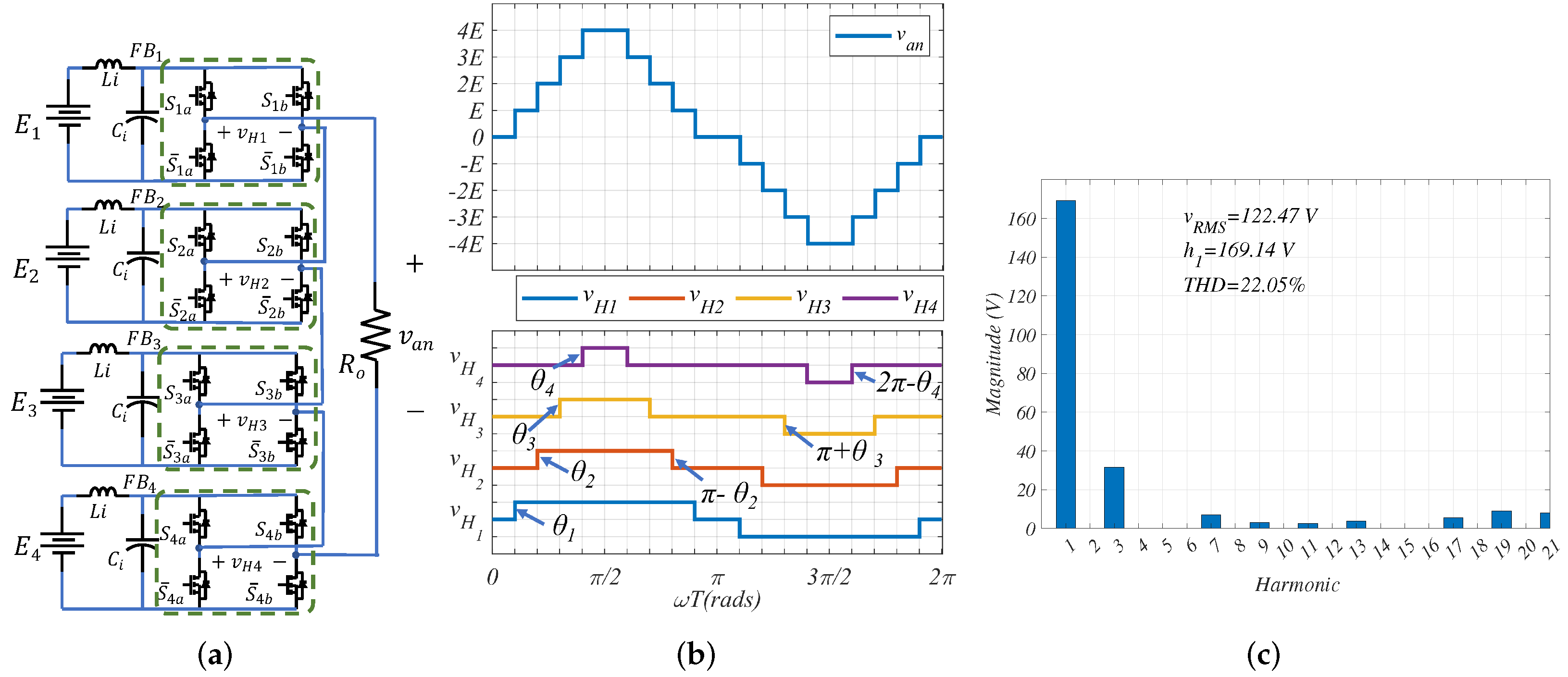
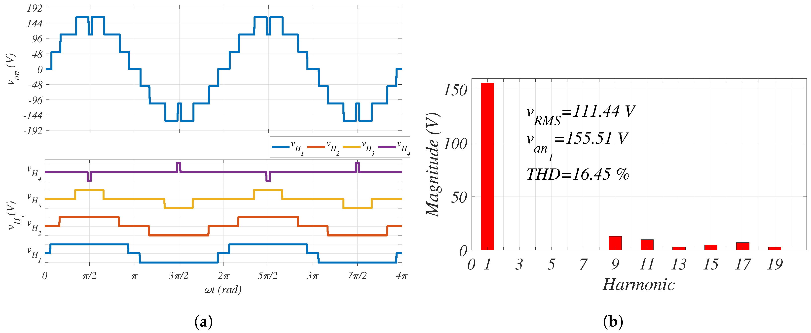
The proposed work describes an adaptive modulation technique for selective harmonic elimination applied to a multilevel inverter, using 4-cells maximum. This limitation will be explained at the end of Section 3. The system described in this article corresponds to a Cascaded Full-Bridge Multilevel Inverter (CFBMI), composed of 4 Full-Bridge Cells (FBC), as shown in Figure 1a, where $E_k$ and $v_{H_k}$ are the input and output voltages of the $k^{th}$ FBC ($F{B}_k$), respectively, for $k=\{1,2,3,4\}$. $v_{an}$ is the output voltage of the entire system, corresponding to the sum of all the $v_{H_k}$. In this work, each FBC switches once per quarter of the cycle. The aims are to control the fundamental component and to eliminate as many harmonics as possible. Figure 1b shows the waveform of the output voltage, neglecting the effects of inductors and capacitors of the input filters, and Figure 1c shows the harmonics analysis of the produced waveform when all the switching-angles are equally separated (${\theta }_k=2\pi k/5$).

Notice that the waveforms are symmetric in both axes, as $F{B}_k$ commutes at ${\theta }_k,\pi -{\theta }_k,\pi +{\theta }_k,$ and $2\pi -{\theta }_k$, producing that the even order harmonics and the quadrature components of all the harmonics are eliminated as it is mentioned in [17,23,24]. Furthermore, it can be observed that if there is no specific control law for the computation of the switching-angles, harmonics at different orders are produced as shown in Figure 1c.

2.1. Computing the Output Voltage Harmonics

In this subsection, an analytical expression of the harmonics, as a function of the switching-angles is obtained. Based on Figure 1b, the Fourier components of $v_{H_k}$ are defined as:

$$v_{H_k}=\sum _{l=1}^{\infty }\left(b_{kl}sin\left(l\omega t\right)+a_{kl}cos\left(l\omega t\right)\right)$$

(1)

As mentioned previously, all the quadrature components and the even order harmonics are eliminated. Hence the $l^{th}$ Fourier coefficient of the $k^{th}$ FBC can be described as:

$$\begin{array}{cc}\hfill b_{kl}=& \left\{\begin{array}{ccc}\frac{4E_k}{l\pi }cos\left(l{\theta }_k\right)& ;& l\mathrm{is}\mathrm{odd};\forall k=\{1,2,3,4\}\\ 0& ;& l\mathrm{is}\mathrm{even};\forall k=\{1,2,3,4\}\end{array}\right.\hfill \end{array}$$

(2a)

$$\begin{array}{cc}\hfill a_{kl}=& \begin{array}{ccc}0& ;& \forall k=\{1,2,3,4\};\forall l\ge 1\end{array}\hfill \end{array}$$

(2b)

Then, defining $v_{an}$ as the sum of all the $v_{H_k}$:

$$\begin{array}{c}{v}_{an}=\frac{4}{\pi }{\displaystyle \sum _{l=1}^{\infty }}\left(\frac{1}{l}{\displaystyle \sum _{k=1}^4}\left(E_{k}cos\left(l{\theta }_k\right)\right)sin\left(l\omega t\right)\right)\\ \end{array}$$

(3)

According to (3), the $l^{th}$ Fourier components ($h_l$) of $v_{an}$ is defined as:

$$h_l=\frac{4}{l\pi }\sum _{k=1}^4\left(E_{k}cos\left(l{\theta }_k\right)\right)$$

(4)

Assuming that all the sources are identical, the nominal value of $E_k$ is noted E. Therefore, $E_k$ can be defined as $E_k=E(1+{\delta }_k)$, ${\delta }_k$ is a disturbance in the input voltage E. Then, defining $h_l^{\prime }$ as:

$$h_l^{\prime }=\frac{h_l}{E}$$

(5)

It follows,

$$h_l^{\prime }=\frac{4}{l\pi }\sum _{k=1}^4(1+{\delta }_k)cos\left(l{\theta }_k\right)$$

(6)

Knowing that $cos\left(l\theta \right)=T_l(cos\left(\theta \right))$ where $T_l(•)$ is the Chebyshev polynomial of first kind of $l^{th}$ degree, then:

$$h_l^{\prime }=\frac{4}{l\pi }\sum _{k=1}^4(1+{\delta }_k)T_l\left(x_k\right)$$

(7)

where $x_k=cos\left({\theta }_k\right)$.

As it is mentioned previously, this strategy aims to impose the fundamental component and to eliminate the most significant harmonics. In this work, those correspond to the first three odd order harmonics. For that reason, expanding $T_l\left(x_k\right)$ for $l=\{1,3,5,7\}$:

$$\begin{array}{cc}\hfill h_1^{\prime }& ={\displaystyle \frac{4}{\pi }}\sum _{k=1}^4(1+{\delta }_k)x_k\hfill \\ \hfill h_3^{\prime }& ={\displaystyle \frac{4}{3\pi }}\sum _{k=1}^4(1+{\delta }_k)\left(4x_k^3-3x_k\right)\hfill \\ \hfill h_5^{\prime }& ={\displaystyle \frac{4}{5\pi }}\sum _{k=1}^4(1+{\delta }_k)\left(16x_k^5-20x_k^3+5x_k\right)\hfill \\ \hfill h_7^{\prime }& ={\displaystyle \frac{4}{7\pi }}\sum _{k=1}^4(1+{\delta }_k)\left(64x_k^7-112x_k^5+56x_k^3-7x_k\right)\hfill \end{array}$$

(8)

Expressing (8) as a matrix form:

$${\mathbf{H}}_{\mathbf{R}}^{\prime }=\Pi \left(\mathbf{X}\right)({\mathbf{V}}_{\mathbf{1}}+\Delta )$$

(9)

where ${\mathbf{V}}_{\mathbf{1}}={\left[\begin{array}{cccc}1& 1& 1& 1\end{array}\right]}^T$, ${\mathbf{H}}_{\mathbf{R}}^{\prime }={\left[\begin{array}{cccc}{h}_1^{\prime }& h_2^{\prime }& h_3^{\prime }& h_4^{\prime }\end{array}\right]}^T$, $\Delta ={\left[\begin{array}{cccc}{\delta }_1& {\delta }_2& {\delta }_3& {\delta }_4\end{array}\right]}^T$, $\mathbf{X}={\left[\begin{array}{cccc}{x}_1& x_2& x_3& x_4\end{array}\right]}^T$,

$$\Pi \left(\mathbf{X}\right)=\begin{array}{c}\frac{4}{\pi }\left[\begin{array}{cccc}{T}_1\left(x_1\right)& T_1\left(x_2\right)& T_1\left(x_3\right)& T_1\left(x_4\right)\\ \frac{1}{3}{T}_3\left(x_1\right)& \frac{1}{3}{T}_3\left(x_2\right)& \frac{1}{3}{T}_3\left(x_3\right)& \frac{1}{3}{T}_3\left(x_4\right)\\ \frac{1}{5}{T}_5\left(x_1\right)& \frac{1}{5}{T}_5\left(x_2\right)& \frac{1}{5}{T}_5\left(x_3\right)& \frac{1}{5}{T}_5\left(x_4\right)\\ \frac{1}{7}{T}_7\left(x_1\right)& \frac{1}{7}{T}_7\left(x_2\right)& \frac{1}{7}{T}_7\left(x_3\right)& \frac{1}{7}{T}_7\left(x_4\right)\end{array}\right]\end{array}$$

Equation (9) expresses the Fourier components that are managed as a function of the cosine of the switching-angles defined as $\mathbf{X}$. Lets define ${\mathbf{H}}_{\mathbf{e}}^{\prime }$, as the estimated harmonics, corresponding to the harmonics with no disturbances. Hence:

$${\mathbf{H}}_{\mathbf{e}}^{\prime }=\Pi \left(\mathbf{X}\right){\mathbf{V}}_{\mathbf{1}}$$

(10)

Notice that if there is no disturbance, it follows ${\mathbf{H}}_{\mathbf{R}}^{\prime }={\mathbf{H}}_{\mathbf{e}}^{\prime }$. The next subsection shows a method to solve (10).

2.2. Solving the Polynomial Equation

To solve (10), this paper uses an algebraic method that converts (10) into its Groebner Basis. The groebner basis conversion is developed in Maple. There exists several algorithm for that. However, the most used, the most efficient and also compact to use is the Buchberger’s Algorithm [29] which consists in developing several polynomial divisions to meet a predefined condition. The resulting system is another polynomial system of equations with the same solution set where the coefficients of the variables are polynomial functions of ${\mathbf{H}}_{\mathbf{e}}^{\prime }$ following the form:

$$\begin{array}{cc}\hfill p_1(x_1,{\mathbf{H}}_{\mathbf{e}}^{\prime })& =0\hfill \\ \hfill p_2(x_1,x_2,{\mathbf{H}}_{\mathbf{e}}^{\prime })& =0\hfill \\ \hfill ⋮& \\ \hfill p_N(x_1,x_2,\cdots x_N,{\mathbf{H}}_{\mathbf{e}}^{\prime })& =0\hfill \end{array}$$

(11)

This conversion decouples the independent variables, simplifying the solving process of the system. Refs. [23,29] explain this polynomial conversion. Furthermore, according to [17], this system corresponds to a symmetric polynomial system, meaning that the solution set of any $x_k$ is a permutation of the solution set of $x_1$. For that reason, finding the solution set of $p_1(x_1,{\mathbf{H}}^{\prime }\mathbf{e})$, the solution set of the other $x_k$ is also found. Therefore, it is possible to define the system as:

$$\begin{array}{cc}\hfill q(x_1,{\mathbf{H}}_{\mathbf{e}}^{\prime })& =0\hfill \\ \hfill ⋮& \\ \hfill q(x_N,{\mathbf{H}}_{\mathbf{e}}^{\prime })& =0\hfill \end{array}$$

(12)

where $q(x_k,{\mathbf{H}}_{\mathbf{e}}^{\prime })=p_1(x_k,{\mathbf{H}}_{\mathbf{e}}^{\prime })$.

Grouping (12), it follows:

$$\mathbf{Q}(\mathbf{X},{\mathbf{H}}_{\mathbf{e}}^{\prime })=0$$

(13)

where $\mathbf{Q}(\mathbf{X},{\mathbf{H}}_{\mathbf{e}}^{\prime })$ represents all the polynomials obtained by the Groebner basis conversion.

Equation (14) describes $q(x_k,{\mathbf{H}}_{\mathbf{e}}^{\prime })$, where its roots corresponds to the solution set of all the cosine of the switching-angles.

$$\begin{array}{cc}\hfill & (268.8{\pi }^4{h_1^{\prime }}^6-16128{\pi }^2{h_1^{\prime }}^4-16128{\pi }^2{h_1^{\prime }}^3{h}_3^{\prime }+193536{h_1^{\prime }}^2+193536h_1^{\prime }{h}_3^{\prime }+193536h_1^{\prime }{h}_5^{\prime }-193536{h_3^{\prime }}^2)x_k^4\hfill \\ & -(67.2{\pi }^5{h_1^{\prime }}^7-4032{\pi }^3{h_1^{\prime }}^5-4032{\pi }^3{h_1^{\prime }}^4{h}_3^{\prime }+48384\pi {h_1^{\prime }}^3+48384\pi {h_1^{\prime }}^2{h}_3^{\prime }+48384\pi {h_1^{\prime }}^2{h}_5^{\prime }-48384\pi h_1^{\prime }{h_3^{\prime }}^2)x_k^3\hfill \\ & +(720{\pi }^6{h_1^{\prime }}^8-604.8{\pi }^4{h_1^{\prime }}^6-604.8{\pi }^4{h_1^{\prime }}^5{h}_3^{\prime }+16128{\pi }^2{h_1^{\prime }}^4+24192{\pi }^2{h_1^{\prime }}^3{h}_3^{\prime }+8064{\pi }^2{h_1^{\prime }}^3{h}_5^{\prime }-145152{h_1^{\prime }}^2\hfill \\ & -193536h_1^{\prime }{h}_3^{\prime }-193536h_1^{\prime }{h}_5^{\prime }-48384h_1^{\prime }{h}_7^{\prime }+145152{h_3^{\prime }}^2+48384h_3^{\prime }{h}_5^{\prime })x_k^2-(40{\pi }^7{h_1^{\prime }}^9-50.4{\pi }^5{h_1^{\prime }}^7-50.4{\pi }^5{h_1^{\prime }}^6{h}_3^{\prime }\hfill \\ & -2016{\pi }^3{h_1^{\prime }}^5+3024{\pi }^3{h_1^{\prime }}^4{h}_3^{\prime }+1008{\pi }^3{h_1^{\prime }}^4{h}_5^{\prime }-24192\pi {h_1^{\prime }}^3-24192\pi {h_1^{\prime }}^2{h}_3^{\prime }+36288\pi {h_1^{\prime }}^2{h}_5^{\prime }+12096\pi {h_1^{\prime }}^2{h}_7^{\prime }\hfill \\ & +36288\pi h_1^{\prime }{h_3^{\prime }}^2-24192\pi h_1^{\prime }{h}_3^{\prime }{h}_5^{\prime }+12096\pi {h_3^{\prime }}^3)x_k+{\pi }^8{h_1^{\prime }}^{10}-1.8{\pi }^6{h_1^{\prime }}^8-1.8{\pi }^6{h_1^{\prime }}^7{h}_3^{\prime }+100.8{\pi }^4{h_1^{\prime }}^6\hfill \\ & +151.2{\pi }^4{h_1^{\prime }}^5{h}_3^{\prime }+50.4{\pi }^4{h_1^{\prime }}^5{h}_5^{\prime }-2016{\pi }^2{h_1^{\prime }}^4-3024{\pi }^2{h_1^{\prime }}^3{h}_3^{\prime }-2016{\pi }^2{h_1^{\prime }}^3{h}_5^{\prime }-1008{\pi }^2{h_1^{\prime }}^3{h}_7^{\prime }+3024{\pi }^2{h_1^{\prime }}^2{h}_3^{\prime }{h}_5^{\prime }\hfill \\ & -30.24{\pi }^2{h}_1^{\prime }{h_3^{\prime }}^3+120.96{h_1^{\prime }}^2+24192h_1^{\prime }{h}_3^{\prime }+12096h_1^{\prime }{h}_5^{\prime }+12096h_7^{\prime }{h}_1^{\prime }-12096h_3^{\prime }{h}_5^{\prime }+12096h_3^{\prime }{h}_7^{\prime }-12096{h_5^{\prime }}^2=0\hfill \end{array}$$

(14)

3. Analysis of the Solutions

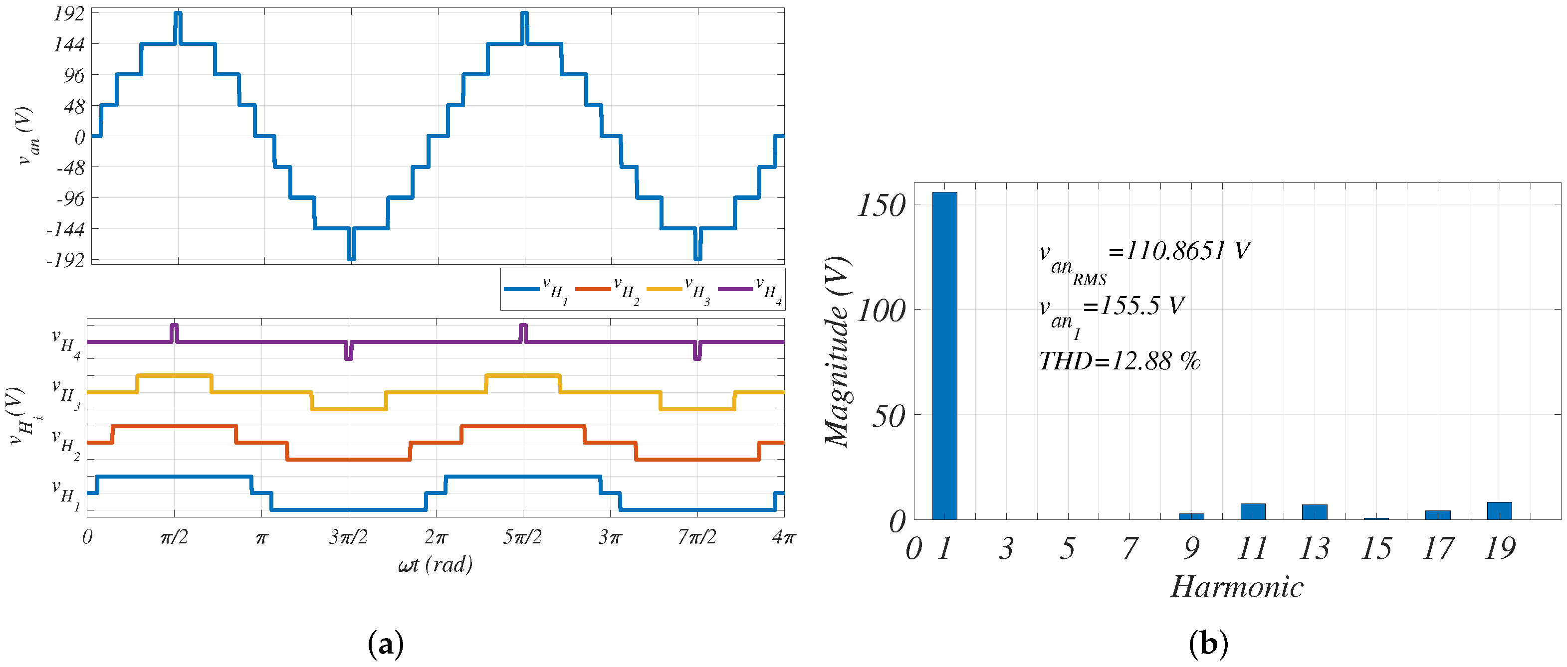
To validate the Groebner conversion described in (14), the parameters are set to $E=48$ V, $h_1=155$ V. Therefore, according to (5), $h_{e_1}^{\prime }=3.23$. Furthermore, taking into account that the objective is to eliminate the third, fifth and seventh order harmonics ($h_3,h_5$ and $h_7$). Those harmonics are equaled to 0. Based on these parameters, the solution set of (14) is: $x_1=0.9842,x_2=0.8958,x_3=0.6187,x_4=0.0468$, resulting the switching-angles: ${\theta }_1=0.1780$ rad, ${\theta }_2=0.4606$ rad, ${\theta }_3=0.9037$ rad, ${\theta }_4=1.5240$ rad. Figure 2a shows the waveform of $v_{an}$, $v_{H_1},v_{H_2},v_{H_3}$ and $v_{H_4}$ with the respective switching-angles, and Figure 2b shows the Harmonics analysis.

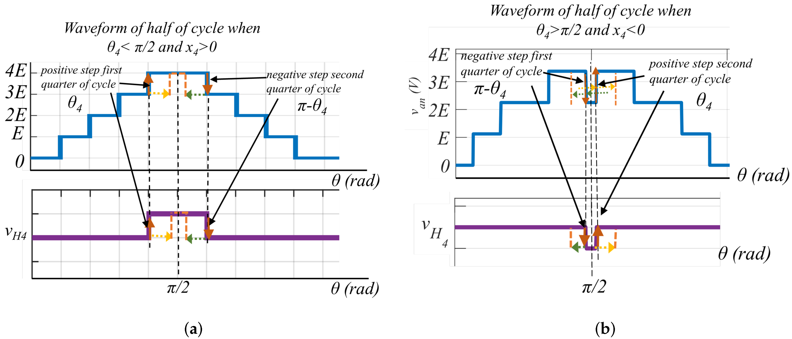
Comparing Figure 1c and Figure 2b it is shown that the third, fifth and seventh order harmonics are eliminated, while the fundamental value is the desired one. Furthermore, Figure 2a shows that all the FBCs present a positive step in the first quarter of the cycle. However, for different values of $h_1$, $x_k$ can be negatives or higher than one. When $x_k$ is negative, the switching-angle is higher than $\pi /2$, producing a negative step. Figure 3a shows the behavior of the waveform when $x_k$ is positive and Figure 3b shows the output voltage when $x_4<0$.

According to Figure 2a and Figure 3a when all the switching-angles are lower than $\pi /2$, all the $x_k$ values are positives, presenting the levels: 4E, 3E, 2E, E, 0, −E, −2E, −3E, −4E; meaning that for this case the $v_{an}$ has 9 levels.

For the case of Figure 3b, which shows the waveform of $v_{an}$ and $v_{H4}$ when $x_4<0$, it can be inferred that the $v_{an}$ has the following levels: 3E, 2E, E, 0 E, 2E, 3E; meaning that for one $x_k$ value less than zero, the $v_{an}$ presents seven levels, two levels less than the previous case, one level less for the positive part and one less for the negative one. Hence, if E is high enough, it is possible to remove the third, fifth and seventh order harmonics, having the same fundamental component with less than nine levels, switching four times per quarter of the cycle. Thus, it is possible to deduce that the number of levels is not relevant in the solution and only the number of commutations per quarter of cycles and the value of E care. It should be noted that having more levels than switching-angles is equivalent to have asymmetric levels with steps of more than twice the minimum level.

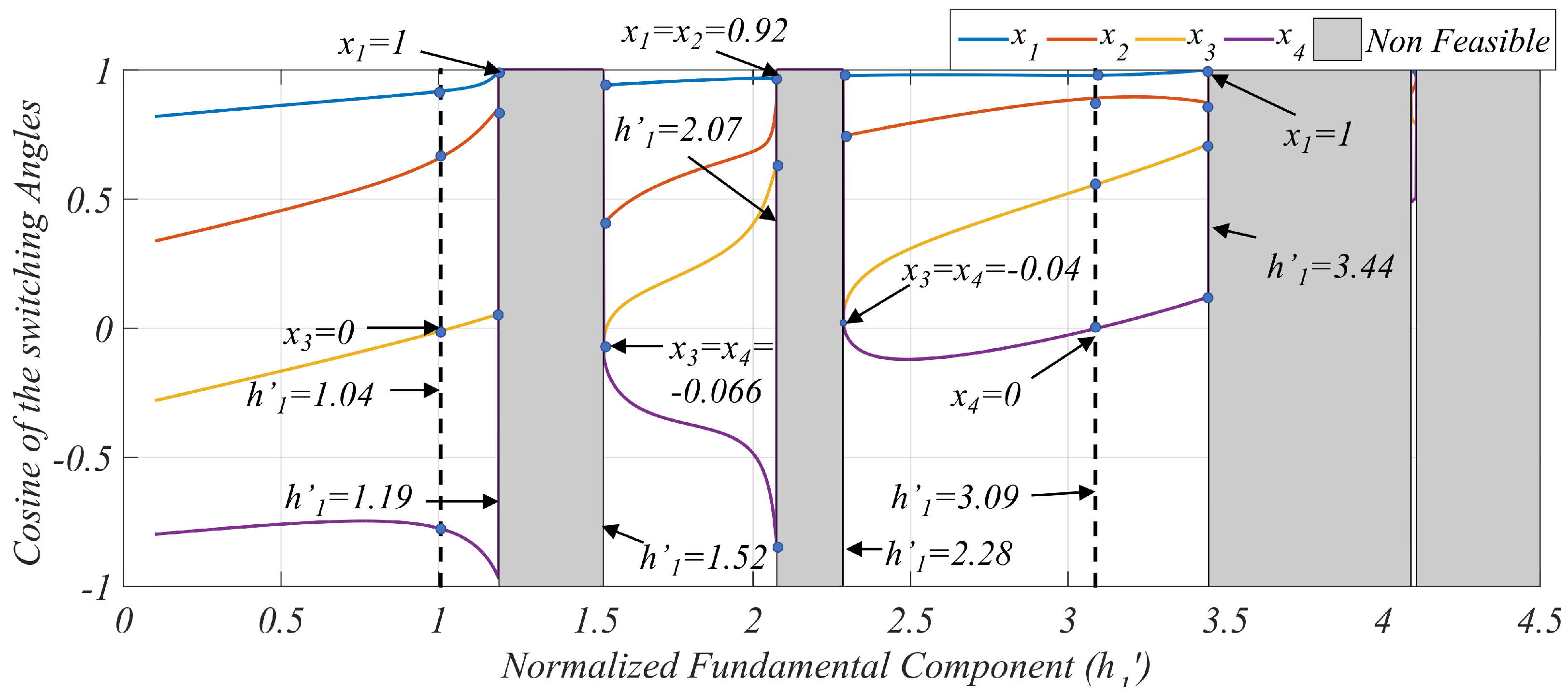
In other cases, depending on $h_1^{\prime }$, the solution set of (14) can present complex values, higher than 1 or lower than -1. Then, there are no switching-angles that satisfy the desired $h_{e_1}^{\prime }$ and the nullity of $h_{e_3}^{\prime },h_{e_5}^{\prime },h_{e_7}^{\prime }$. To analyze the behavior of the solution set when the system eliminates $h_{e_3}^{\prime },h_{e_5}^{\prime }$ and $h_{e_7}^{\prime }$, Figure 4 shows $\mathbf{X}$ vs $h_{e_1}^{\prime }$ when the third, fifth and seventh order harmonics are zero.

Note that there are three regions where a feasible solution of the system does not exist: $1.19<h_{e1}^{\prime }<1.52$; $2.07<h_{e1}^{\prime }<2.28$ and $h_{e1}^{\prime }>3.44$. Figure 4 also shows that in other regions, the values of $x_k$ are negative, meaning that the step is negative in the positive semi cycle. This paper focuses in the feasible region $2.28<h_{e1}^{\prime }<3.44$, because in this region the maximum number of levels (9) with 4 FBCs is generated. In this region only $x_4$ can be negative, meaning that it is possible to produce 7 or 9 levels, according to the value of the fundamental component.

To prove that the Groebner conversion is valid for cases where $x_4<0$, Figure 5a shows $v_{an}$ and $v_{H_k}$ when $E=54$ V and $h_1=155.5$ V. With these parameters, $h_{e_1}^{\prime }=2.88$ and the solution set of $\mathbf{X}$ is: $x_1=0.9797,x_2=0.8661,x_3=0.4744,x_4=-0.0582$, generating the switching-angles of: ${\theta }_1=0.2020$ rad, ${\theta }_2=0.5235$ rad, ${\theta }_3=1.0765$ rad, ${\theta }_4=1.629$ rad. Note that ${\theta }_4>\pi /2$ means that the step in $F{B}_4$ is negative during the first quarter of cycle. Notice in Figure 5a that $v_{H_4}$ starts with a negative step and $v_{an}$ has 2 levels less than the $v_{an}$ shown in Figure 2a. To validate this result, Figure 5b shows the Harmonic analysis of Figure 5a, where the fundamental component does not change and the third, fifth and seventh order harmonics, $h_{e_3}^{\prime },h_{e_5}^{\prime },h_{e_7}^{\prime }$, are eliminated again.

This result indicates that it is possible to analyze mathematically this system according to the number of switching-angles without taking into account the number of FBCs, knowing that $x_k>0$ and $x_k<0$ produces positive and negative step the first quarter of cycle, respectively.

Apparently, this method could work for any number of switching-angles. However, for more than 4 commutations per quarter of cycle, the software never find the Groebner basis. This is because it is necessary to express the coefficients of the Groebner basis as a function of the harmonics; and those are found solving another polynomial equation. If the degree of this polynomial equation is higher than four, according to Galois theory, it is not possible to find its roots in a explicit manner [26].

4. Closing the Loop

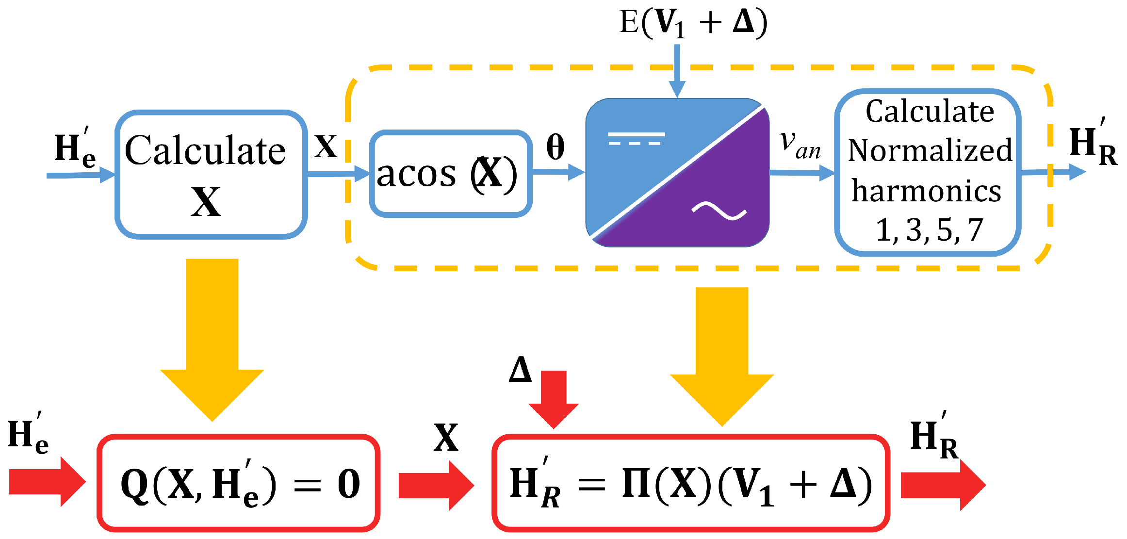
In this section, a control law is proposed to ensure a desired fundamental component and the elimination of the selected harmonics when a disturbance occurs. According to (9) and (13), the system is modeled as a static one. The proposed computation method consists of two steps. The first one corresponding to (13), indicates that for a given estimated harmonics, ${\mathbf{H}}_{\mathbf{e}}$, the polynomial $\mathbf{Q}(\mathbf{X},{\mathbf{H}}_{\mathbf{e}}^{\prime })$ provides a solution set for $\mathbf{X}$. Then in the second step, modeled by (9), the switching-angles ${\theta }_k$ are obtained from $\mathbf{X}$ and applied to the inverter, generating the output voltage, $v_{an}$. Then, the normalized harmonics of $v_{an}$, ${\mathbf{H}}_{\mathbf{R}}^{\prime }$, are computed. Figure 6 shows a diagram of the implemented system and the static model that represents it.

The model shown in Figure 6 is static, nonlinear, and presents an implicit system Equation (13). However, for designing a controller aimed to cancel some specific harmonics, it is necessary to obtain an explicit, dynamic model. To achieve these requirements, a Newton Raphson (NR) method with modifications is shown in (15).

$$\overline{){\mathbf{Q}}_t}\stackrel{0}{=}{\mathbf{Q}}_{\mathbf{t}-\mathbf{1}}+\left({\left.\frac{\partial \mathbf{Q}}{\partial \mathbf{X}}\right|}_{t-1}\right)\left({\mathbf{X}}_t-{\mathbf{X}}_{t-1}\right)+\left({\left.\frac{\partial \mathbf{Q}}{\partial {\mathbf{H}}_{\mathbf{e}}^{\prime }}\right|}_{t-1}\right)\left({\mathbf{H}}_{\mathbf{e}t}^{\prime }-{\mathbf{H}}_{\mathbf{e}t-1}^{\prime }\right)$$

(15)

Hence,

$${\mathbf{X}}_t={\mathbf{X}}_{t-1}-{\left({\left.\frac{\partial \mathbf{Q}}{\partial \mathbf{X}}\right|}_{t-1}\right)}^{-1}{\mathbf{Q}}_{t-1}+{\left({\left.\frac{\partial \mathbf{Q}}{\partial \mathbf{X}}\right|}_{t-1}\right)}^{-1}\left({\left.\frac{\partial \mathbf{Q}}{\partial {\mathbf{H}}_{\mathbf{e}}^{\prime }}\right|}_{t-1}\right)\left({\mathbf{H}}_{\mathbf{e}t}^{\prime }-{\mathbf{H}}_{\mathbf{e}t-1}^{\prime }\right)$$

(16)

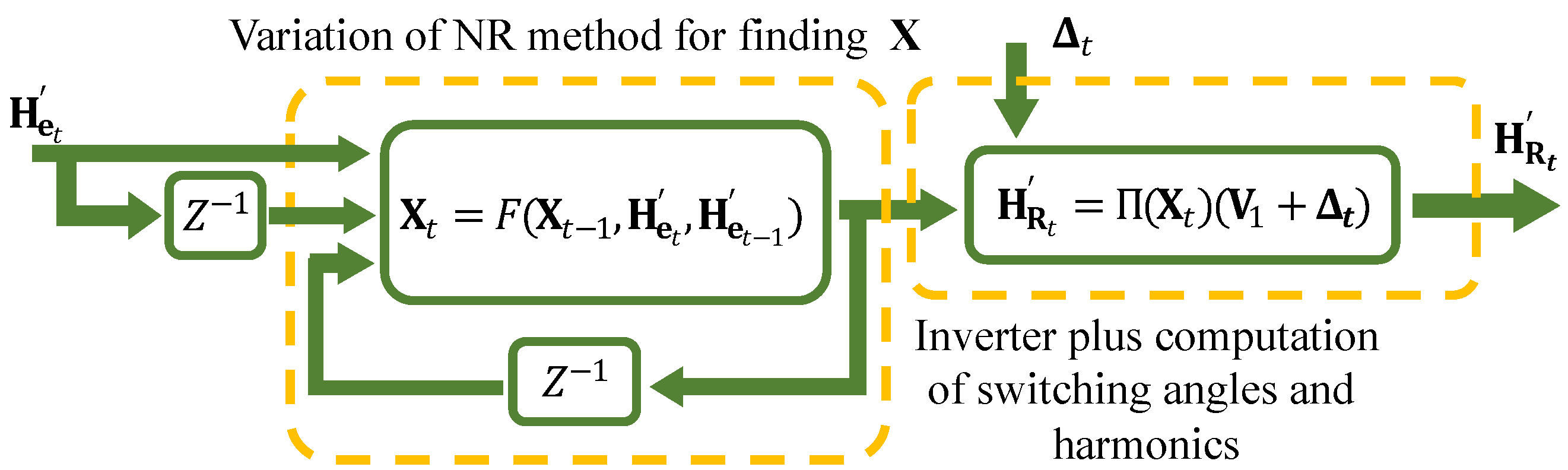
According to (16), if the harmonics do not change, the equation corresponds to the solving process of the classical NR method. Hence, the new system corresponds to a “virtual" dynamical system, composed of two stages. The first one corresponds the iterative equation that solves $\mathbf{X}$, while the second stage corresponds to the static, explicit equation that represents the inverter, the computations of the switching-angle from $\mathbf{X}$ and the computation of the normalized harmonics ${\mathbf{H}}_{\mathbf{R}}^{\prime }$ from the sensed output voltage $v_{an}$. Equation (17) shows the proposed dynamical model of the system and a block diagram of (17) is shown in Figure 7.

$$\left[\begin{array}{c}{\mathbf{X}}_t\\ {\mathbf{H}}_{\mathbf{R}t}^{\prime }\end{array}\right]=\left[\begin{array}{c}F({\mathbf{X}}_{t-1},{\mathbf{H}}_{\mathbf{e}t}^{\prime },{\mathbf{H}}_{\mathbf{e}t-1}^{\prime })\\ \Pi \left({\mathbf{X}}_t\right)({\mathbf{V}}_{\mathbf{1}}+\Delta )\end{array}\right]$$

(17)

Based on this model, the proposed control law is composed of the desired normalized harmonics plus a discrete PI controller, as shown by (18).

$${\mathbf{H}}_{\mathbf{e}t}^{\prime }={\mathbf{H}}_{\mathbf{ref}}^{\prime }+a_1{\xi }_t-a_0{\xi }_{t-1}$$

(18)

where ${\xi }_t={\mathbf{H}}_{\mathbf{ref}}-{\mathbf{H}}_{\mathbf{R}t}$.

Inserting the PI controller in (16), it follows:

$$\begin{array}{cc}\hfill {\mathbf{X}}_t=& {\mathbf{X}}_{t-1}-{\left({\left.\frac{\partial \mathbf{Q}}{\partial \mathbf{X}}\right|}_{t-1}\right)}^{-1}{\mathbf{Q}}_{t-1}-{\left({\left.\frac{\partial \mathbf{Q}}{\partial \mathbf{X}}\right|}_{t-1}\right)}^{-1}\left({\left.\frac{\partial \mathbf{Q}}{\partial {\mathbf{H}}_{\mathbf{e}}^{\prime }}\right|}_{t-1}\right)\left(a_1{\mathbf{H}}_{\mathbf{R}t}^{\prime }-\right.\left.\left(a_1+a_0\right){\mathbf{H}}_{\mathbf{R}t-1}^{\prime }+a_0{\mathbf{H}}_{\mathbf{R}t-2}^{\prime }\right)\hfill \end{array}$$

(19)

where ${\mathbf{H}}_{\mathbf{R}t}=\Pi \left({\mathbf{X}}_t\right)({\mathbf{V}}_{\mathbf{1}}+\Delta )$

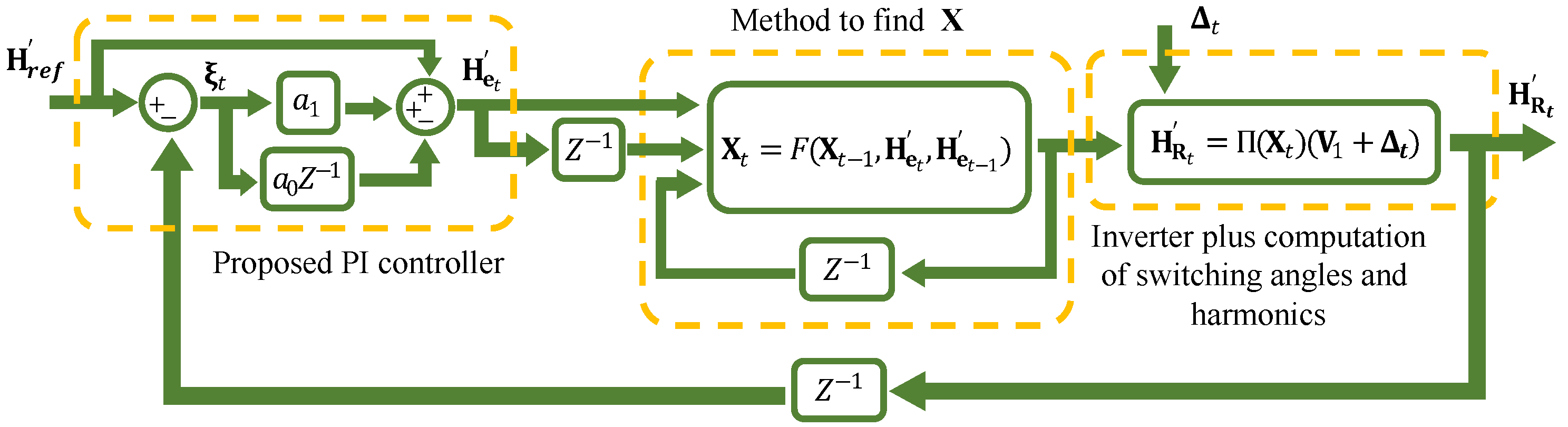
It can be observed that when the angles are found, ${\mathbf{Q}}_{\mathbf{t}}=0$ and the harmonics do not change. Hence, $\mathbf{X}$ does not change, meaning that the system reaches a stable operating point. It should be mentioned that the controller works only in the feasible regions of Figure 4 without passing from one feasible region to another one. Figure 8 shows the block diagram of the closed-loop system. To validate this control law, the next section shows the simulation and experimental results.

5. Results

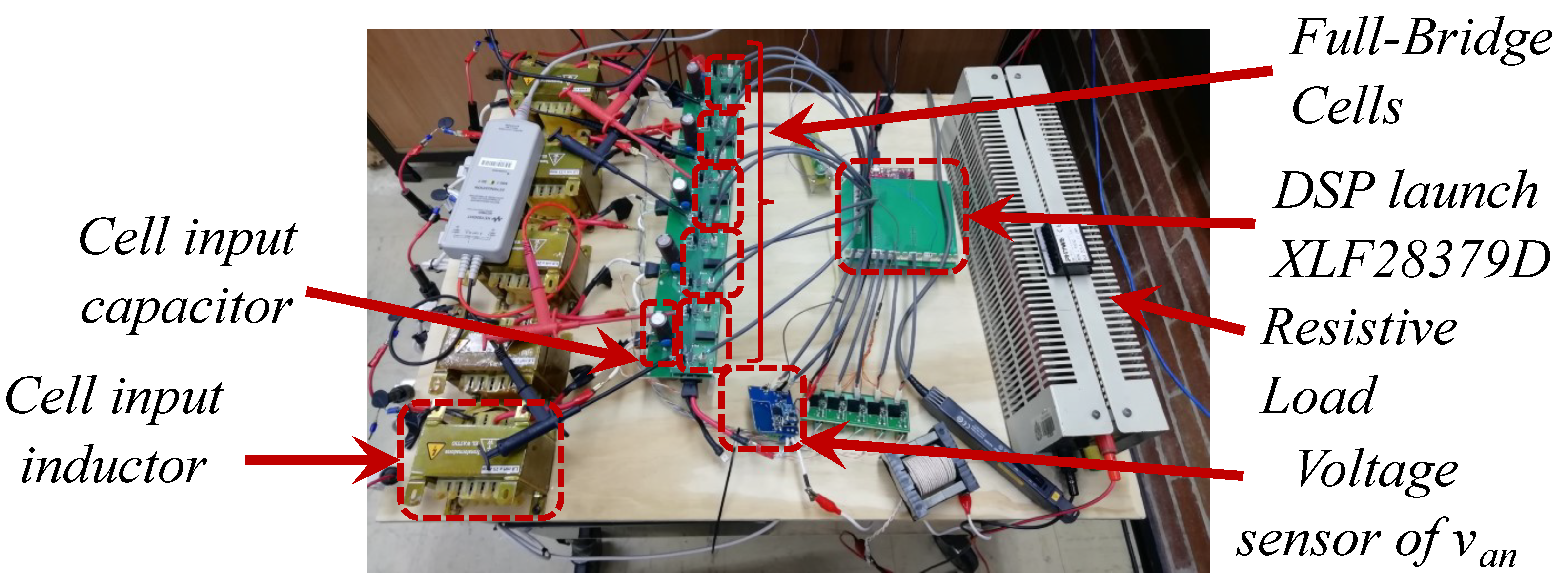
This section develops and comments the obtained simulation and the experimental results. The tests are carried out using the prototype shown in Figure 9, with the parameters described in

Table 1. Parameters of the inverter.

Parameter	Value	Parameter	Value
E	48 V	$R_x$	100 m$\Omega$
$L_i$	$1.8$ mH	$R_o$	$52\Omega$
$R_{L_i}$	200 m$\Omega$	$h_{1_{ref}}$	145 V
$R_s$	200 m$\Omega$	$P_o$	200 W
$C_i$	4 mF	$a_1$	$0.12$
$R_{DS}$	58 m$\Omega$	$a_0$	$0.012$

.

Where the input voltages, E, come from 4 li-ion batteries of 25Ah; $R_{L_k}$ is the DC Resistance (DCR) of the inductance $L_k$, $P_o$ is the output power, $R_{DS}$ is the series ON resistances of the IRFI4212 switches, and the Si8274 is used as the gate driver.

$R_s$ and $R_x$ are the resistances associated with the wires at the input of each FBC, and at the output of the inverter, respectively. For the acquisition of the harmonics, the DSP captures the output voltage during 20 periods of $v_{an}$, with a sampling time of 66 $\mathsf{\mu }$s. Indeed, according to signal processing theory shown in [30], in order to have good accuracy, the period of acquisition must be 10 times higher than the period of the minimum Fourier coefficient. The oscilloscope used correspond to a DSOX3034 of Keysight, which has a bandwidth of 350 MHz. The tests developed hereafter correspond to an insertion of a load and a disturbance in one of the input voltages.

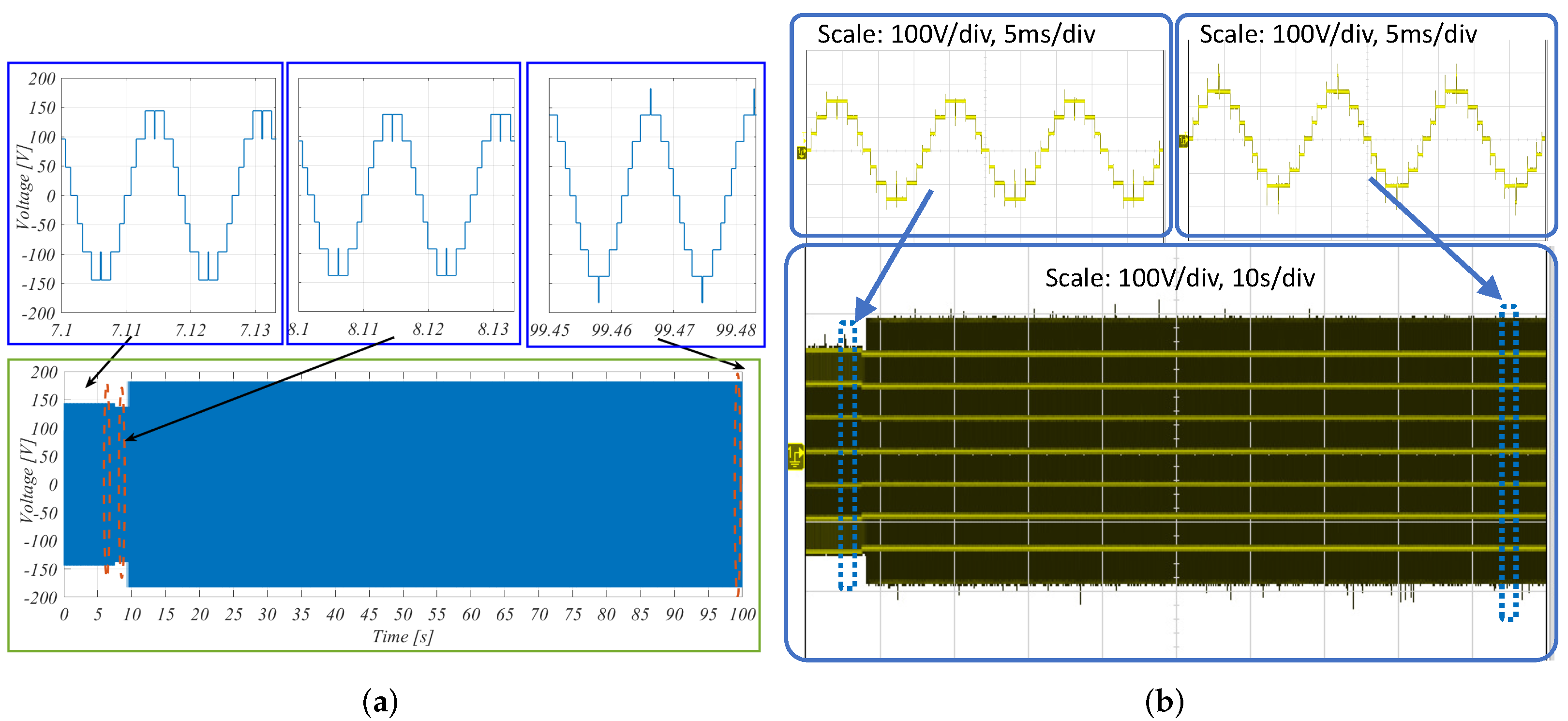
5.1. Response to a Load Transient

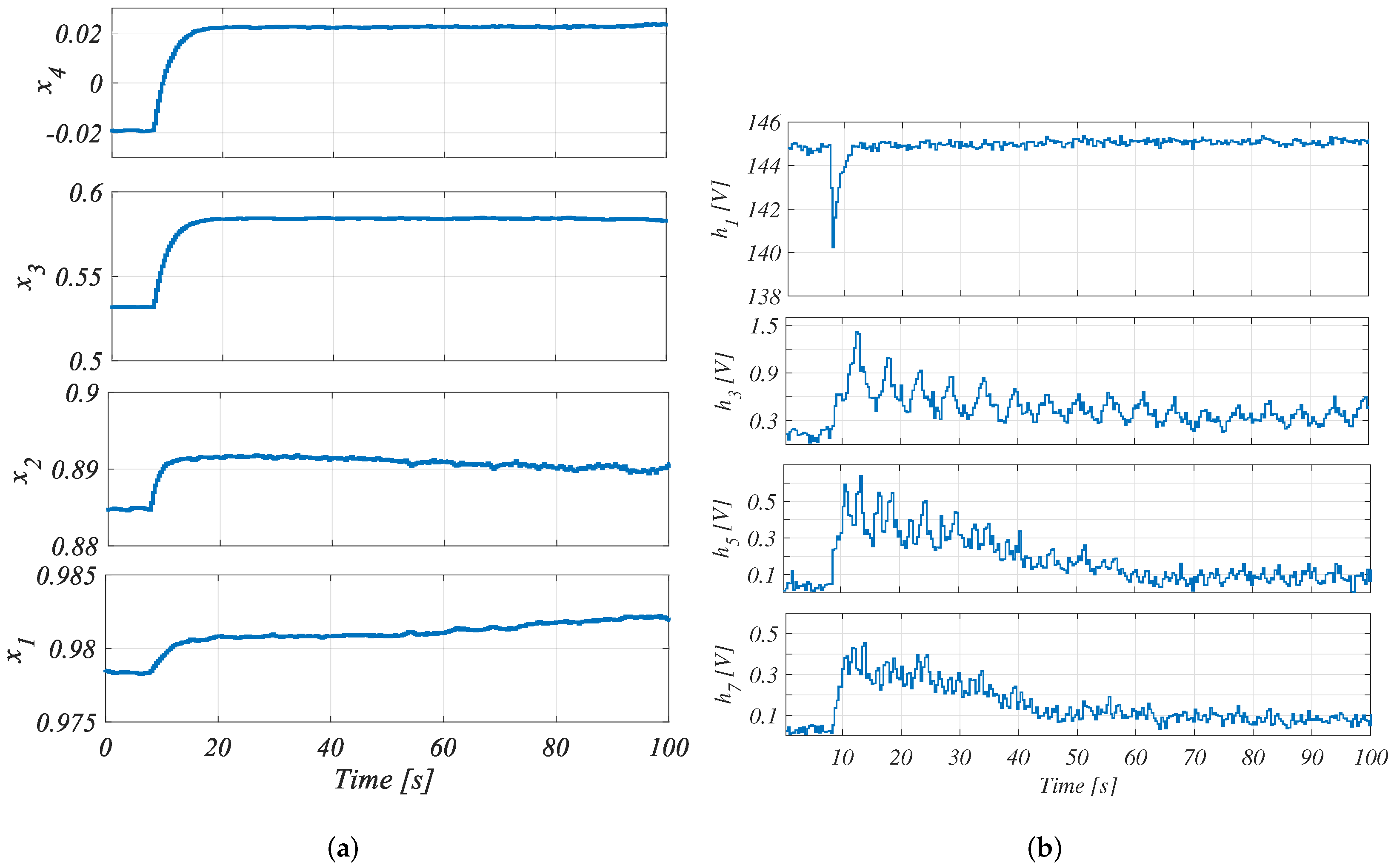
This test analyzes the system when a load of 200 W is inserted at t = 7.5 s. Figure 10a,b show the simulation and experimental results, respectively, validating its similarity. Before the load insertion, one can observe a negative step in $F{B}_4$, because of according to Table 1 and (5), $h_1=145$ V, $E=48$ V and $h_1^{\prime }=3.02$, which produces a negative value of $x_4$, as Figure 4 indicates. When the load is inserted, there is a voltage drop caused by the impedance of the converter. Hence, to regulate the fundamental component, the inverter must produce a higher fundamental component. According to Figure 4, to increase the fundamental component from $h_1^{\prime }=3.02$, it is necessary to increase $x_4$ to reach values higher than 0. For that reason, when the controller acts to regulate the fundamental component and the harmonics, $x_4$ changes from a negative value to a positive value, as shown in Figure 11a. The desired fundamental component is recovered and the third, fifth, and seventh order harmonics are reduced again close to zero volts, as shown in Figure 11b. The fundamental component reaches the reference value in about 6 s. All the selected order harmonics remain between 0 and 1.45 V, meaning they reach a value less than 1% of the fundamental component. After 30 s, these harmonics are less 0.34 % of the fundamental component.

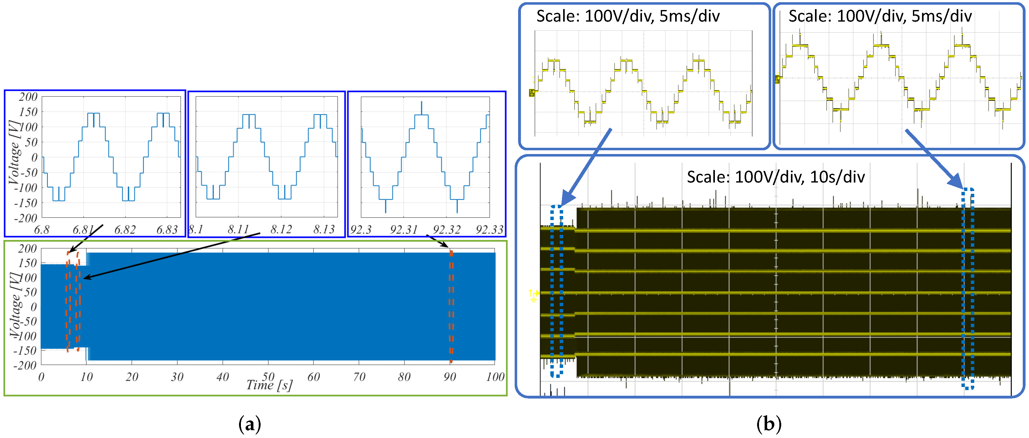
5.2. Disturbance on a Cell Input Voltage Source

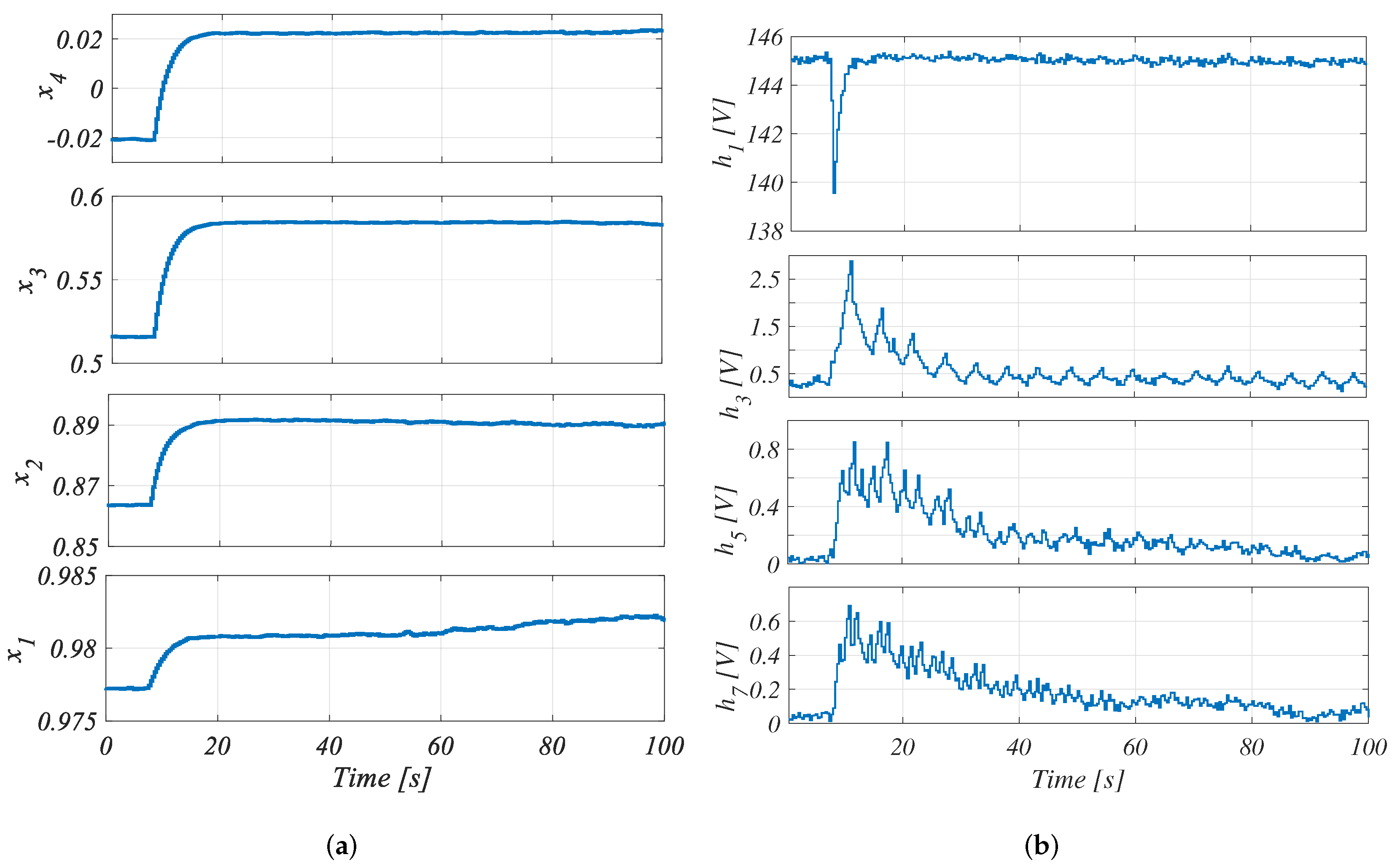
This test shown in Figure 12a,b is carried out with the converter connected to a 200 W load while applying a step transient to $E_1$ from 55 V to 48 V. It should be noted that before the voltage step, the fourth FBC presents a negative step. This is because $E_1$ is higher than the other sources, seven levels being enough, instead of nine, producing a steady-state of $x_4$ lower than 0, while the others $x_k$ are higher than 0, as shown in Figure 13a. When $E_1$ goes back to 48 V, all the $x_k$ are positive, producing a positive step and reaching the desired fundamental component. All the FBs show positive steps because $E_1$ is reduced. For that reason, the inverter presents lower voltage in the inputs. Hence the FBs must increase the value of the fundamental component. Figure 13b shows the behavior of the harmonics during this test, presenting overshoots in $h_1$, $h_3$, $h_5$, that correspond to 4%, 1.1% and 0.4% of the reference of $h_1$, respectively. $h_7$ is almost not affected. $h_1$ is stabilized after 5 s. In this test, the harmonics present a very low oscillations representing 0.48% of the fundamental component in the worst case, validating the robustness of the controller.

6. Conclusions

This article has presented a control law applied to low frequency modulation strategy, regulating the fundamental component and eliminating the third, fifth and seventh order harmonics for the case of a multilevel inverter involving 6 to 8 cells.

Implementing real-time switching angle computations for SHE control method is not common due to its complexity. Using Groebner basis approach to decouple the equations and Newton Rapshon to emulate a virtual dynamical model allows to control the fundamental and harmonics with an additional PI controller. This process relaxes the complexity and saves processing time to compensate the switching-angles if a disturbance in the input voltage or in the load occurs.

This control method is validated both by observing the response of the system during a load transient and disturbing one of the cell input voltage sources, canceling practically the harmonics of third, fifth and seventh order and regulating the fundamental components in all the tests.

Concerning the future works, proving that the proposed controller can operate for a higher number of commutations, meaning eliminating more harmonics, is under investigation. This will allow to use more cells in the multilevel inverters.

References

- Sahoo, S.K.; Bhattacharya, T. Phase-Shifted Carrier-Based Synchronized Sinusoidal PWM Techniques for a Cascaded H-Bridge Multilevel Inverter. IEEE Trans. Power Electron. 2018, 33, 513–524. [Google Scholar] [CrossRef]
- Cousineau, M.; Cougo, B. Interleaved converter with massive parallelization of high frequency GaN switching-cells using decentralized modular analog controller. In Proceedings of the 2015 IEEE Energy Conversion Congress and Exposition (ECCE), Montreal, QC, Canada, 20–24 September 2015; pp. 4343–4350. [Google Scholar] [CrossRef]
- Fabre, J.; Ladoux, P. Parallel Connection of 1200-V/100-A SiC-MOSFET Half-Bridge Modules. IEEE Trans. Ind. Appl. 2016, 52, 1669–1676. [Google Scholar] [CrossRef]
- Vivert, M.; Cousineau, M.; Ladoux, P.; Fabre, J. Decentralized Controller for the Cell-Voltage Balancing of a Multilevel Flying Cap Converter. In Proceedings of the PCIM Europe 2019, International Exhibition and Conference for Power Electronics, Intelligent Motion, Renewable Energy and Energy Management, Nuremberg, Germany, 7–9 May 2019; pp. 1–8. [Google Scholar]
- Fabre, J.; Ladoux, P.; Solano, E.; Gateau, G.; Blaquière, J. Full SiC multilevel chopper for three-wire supply systems in DC electric railways. In Proceedings of the 2016 International Conference on Electrical Systems for Aircraft, Railway, Ship Propulsion and Road Vehicles International Transportation Electrification Conference (ESARS-ITEC), Toulouse, France, 2–4 November 2016; pp. 1–7. [Google Scholar] [CrossRef]
- Fabre, J.; Ladoux, P.; Solano, E.; Gateau, G.; Blaquière, J. MVDC Three-Wire Supply Systems for Electric Railways: Design and Test of a Full SiC Multilevel Chopper. IEEE Trans. Ind. Appl. 2017, 53, 5820–5830. [Google Scholar] [CrossRef]
- Alolah, A.I.; Hulley, L.N.; Shepherd, W. A three-phase neutral point clamped inverter for motor control. IEEE Trans. Power Electron. 1988, 3, 399–405. [Google Scholar] [CrossRef]
- Negash, M.F.; Manthati, U.B. Development of 7-level cascaded H-bridge inverter topology for PV applications. In Proceedings of the International Conference on Electrical, Electronics, and Optimization Techniques, Chennai, Tamil Nadu, India, 3–5 March 2016; pp. 1847–1852. [Google Scholar] [CrossRef]
- Huang, Q.; Huang, A.Q. Feedforward Proportional Carrier-Based PWM for Cascaded H-Bridge PV Inverter. IEEE J. Emerg. Sel. Top. Power Electron. 2018, 6, 2192–2205. [Google Scholar] [CrossRef]
- Luo, F.L.; Ye, H. Multilevel DC/AC Inverters. In Advanced DC/AC Inverters: Aplications in Renewable Energy; CRC Press: Boca Raton, FL, USA, 2013; Chapter 8; pp. 137–154. [Google Scholar]
- Cobaleda, D.B.; Vivert, M.; Diez, R.; Perilla, G.; Patiño, D.; Ruiz, F. Low-Voltage Cascade Multilevel Inverter with GaN Devices for Energy Storage System. In Proceedings of the 13th IEEE International Conference on Power Electronics and Drive Systems, Toulouse, France, 9–12 July 2019. [Google Scholar]
- Liu Yu, F.L. Trinary hybrid 81-level multilevel inverter for motor drive with zero common-mode voltage. IEEE Trans. Ind. Electron. 2008, 55, 1014–1021. [Google Scholar] [CrossRef]
- Edpuganti, A.; Rathore, A.K. A Survey of Low Switching Frequency Modulation Techniques for Medium-Voltage Multilevel Converters. IEEE Trans. Ind. Appl. 2015, 51, 4212–4228. [Google Scholar] [CrossRef]
- Liu, Y.; Hong, H.; Huang, A.Q. Real-Time Algorithm for Minimizing THD in Multilevel Inverters With Unequal or Varying Voltage Steps Under Staircase Modulation. IEEE Trans. Ind. Electron. 2009, 56, 2249–2258. [Google Scholar] [CrossRef]
- Srndovic, M.; Zhetessov, A.; Alizadeh, T.; Familiant, Y.L.; Grandi, G.; Ruderman, A. Simultaneous Selective Harmonic Elimination and THD Minimization for a Single-Phase Multilevel Inverter With Staircase Modulation. IEEE Trans. Ind. Appl. 2018, 54, 1532–1541. [Google Scholar] [CrossRef]
- Kavousi, A.; Vahidi, B.; Salehi, R.; Bakhshizadeh, M.K.; Farokhnia, N.; Fathi, S.H. Application of the Bee Algorithm for Selective Harmonic Elimination Strategy in Multilevel Inverters. IEEE Trans. Power Electron. 2012, 27, 1689–1696. [Google Scholar] [CrossRef]
- Yang, K.; Zhang, Q.; Yuan, R.; Yu, W.; Yuan, J.; Wang, J. Selective Harmonic Elimination With Groebner Bases and Symmetric Polynomials. IEEE Trans. Power Electron. 2016, 31, 2742–2752. [Google Scholar] [CrossRef]
- Ahmed, M.; Sheir, A.; Orabi, M. Real-Time Solution and Implementation of Selective Harmonic Elimination of Seven-Level Multilevel Inverter. IEEE J. Emerg. Sel. Top. Power Electron. 2017, 5, 1700–1709. [Google Scholar] [CrossRef]
- Haghdar, K.; Shayanfar, H.A. Selective Harmonic Elimination With Optimal DC Sources in Multilevel Inverters Using Generalized Pattern Search. IEEE Trans. Ind. Inform. 2018, 14, 3124–3131. [Google Scholar] [CrossRef]
- Routray, A.; Kumar Singh, R.; Mahanty, R. Harmonic Minimization in Three-Phase Hybrid Cascaded Multilevel Inverter Using Modified Particle Swarm Optimization. IEEE Trans. Ind. Informatics 2019, 15, 4407–4417. [Google Scholar] [CrossRef]
- Sahu, N.; Londhe, N.D. Optimization based selective harmonic elimination in multi-level inverters. In Proceedings of the 2017 National Power Electronics Conference (NPEC), Puerto Varas, Chile, 4–7 December 2017; pp. 325–329. [Google Scholar] [CrossRef]
- Kumar, A.; Chatterjee, D.; Dasgupta, A. Harmonic mitigation of cascaded multilevel inverter with non equal DC sources using Hybrid Newton Raphson Method. In Proceedings of the 2017 4th International Conference on Power, Control Embedded Systems (ICPCES), Allahabad, India, 9–11 March 2017; pp. 1–5. [Google Scholar] [CrossRef]
- Yang, K.; Yuan, Z.; Yuan, R.; Yu, W.; Yuan, J.; Wang, J. A Groebner Bases Theory-Based Method for Selective Harmonic Elimination. IEEE Trans. Power Electron. 2015, 30, 6581–6592. [Google Scholar] [CrossRef]
- Yang, K.; Zhang, Q.; Zhang, J.; Yuan, R.; Guan, Q.; Yu, W.; Wang, J. Unified Selective Harmonic Elimination for Multilevel Converters. IEEE Trans. Power Electron. 2017, 32, 1579–1590. [Google Scholar] [CrossRef]
- Sharifzadeh, M.; Vahedi, H.; Portillo, R.; Franquelo, L.G.; Al-Haddad, K. Selective Harmonic Mitigation Based Self-Elimination of Triplen Harmonics for Single-Phase Five-Level Inverters. IEEE Trans. Power Electron. 2019, 34, 86–96. [Google Scholar] [CrossRef]
- Lal, R. Chapter 8: Field Theory, Galois Theory, 8.8 Galois theory for equations. In Algebra 2. Linear Algebra, Galois Theory, Representation theory, Group extensions and Schur Multipliere; Springer: Singapore, 2017. [Google Scholar]
- Zhao, H.; Jin, T.; Wang, S.; Sun, L. A Real-Time Selective Harmonic Elimination Based on a Transient-Free Inner Closed-Loop Control for Cascaded Multilevel Inverters. IEEE Trans. Power Electron. 2016, 31, 1000–1014. [Google Scholar] [CrossRef]
- Yang, K.; Feng, M.; Wang, Y.; Lan, X.; Wang, J.; Zhu, D.; Yu, W. Real-Time switching-angle Computation for Selective Harmonic Control. IEEE Trans. Power Electron. 2019, 34, 8201–8212. [Google Scholar] [CrossRef]
- Cox, D.; Little, J.; O’Shea, D. Ideals, Varieties, and Algorithms: An Introduction to Computational Algebraic Geometry and Commutative Algebra, 2nd ed.; Springer Science & Business Media: Cham, Switzerland, 2015. [Google Scholar] [CrossRef]
- Proakis, J.G.; Manolakis, D.K. Digital Signal Processing, 4th ed.; Prentice Hall: Hoboken, NJ, USA, 2006. [Google Scholar]
Figure 1.
(a) Cascaded-Full-Bridge Multilevel Inverter with 4 FBCs, (b) Waveforms of , and , (c) harmonic analysis of .
Figure 2.
(a) Waveforms of , (b) Harmonics analysis of .
Figure 3.
Waveforms of and , shifting (a) for and , (b) for and .
Figure 4.
Behavior of the cosine of the switching-angles () according to the fundamental component, , when the third, fifth and seventh order harmonics are equal to 0.
Figure 5.
(a) Waveforms of when , (b) Harmonics analysis of of when .
Figure 6.
Static model and block diagram of the system.
Figure 7.
Virtual dynamic model of the system.
Figure 8.
Block diagram of the CFBMI with the solving method of the Groebner basis conversion, the PI controller and the acquisition of the harmonics.
Figure 9.
Prototype.
Figure 10.
(a) Simulation result of 200 W load insertion, (b) Experimental result of 200 W load insertion.
Figure 11.
(a) Cosine of the switching-angles s in 200 W load insertion test, (b) Harmonics behavior after a 200 W load insertion.
Figure 12.
(a) Simulations of disturbance, (b) Experimental result of disturbance.
Figure 13.
(a) Cosine of the switching-angles s in 200 W load insertion test, (b) Harmonics behavior of disturbance experimental test.