Multi-Crack Dynamic Interaction Effect on Oil and Gas Pipeline Weld Joints Based on VCCT

Abstract

In pipelines for transporting oil and gas, multiple cracks often exist in weld joints. The interaction among the cracks should be considered as it directly affects the life span of the pipeline structures. In the current investigation, based on the fluid–solid magnetic coupling model, the virtual crack-closure technique (VCCT) is applied to systematically study the multi-crack dynamic interaction effect on pipeline welds during the crack propagation process. The results show that the existence of an auxiliary crack accelerates the main crack’s propagation. When the auxiliary crack is nearer to the main crack tip, the enhancement effect of the auxiliary crack on the main crack increases. Further, when the initial length of the auxiliary crack increases, the main crack becomes easier to propagate. Two important parameters, the distance between the two interacting crack tips and the initial size of the auxiliary crack, are studied in detail. Their interference effect on the main crack has been quantified, which is very user-friendly for engineers to conduct failure assessment and prevention for oil and gas pipes with multiple cracks at weld joints.

1. Introduction

In the long-distance transportation of oil and gas by pipelines, welded joints are the weak link of the pipeline system. If there are defects, such as cracks in the joints, it creates a huge safety hazard during operation. Under the action of the thermal welding cycle, due to the change of structure and properties of the weld and heat-affected zone, coupled with the influence of stress and diffusible hydrogen, cracks may occur. Especially with the increase in pipeline strength level (such as ×80 grade pipeline steel), wall thickness and pipe diameter, cold cracks are prone to occur when the welded joint is subjected to a large stress state [1,2,3,4,5,6,7]. When the pipelines are under low-temperature environments (such as the China–Kazakhstan pipeline, the western pipeline and the oil and gas pipeline network in the Northeast), the crack initiation and propagation are even more prominent, and, therefore, results in fracture.

Fracture research has become a hot issue, which has attracted the attention of many scholars. Jovanovi’c et al. investigated the effect of material inhomogeneity and temperature on impact toughness and fracture resistance of SA-387 Gr. 91 welded joints. SA-387 Gr. 91 has a more heavily expressed influence of material heterogeneity on impact toughness than A-387 Gr. B. The influence of temperature on impact toughness is similar but more prominent. The influence of material inhomogeneity and the influence of temperature on fracture toughness are also similar to their influence on impact toughness [8]. Macek et al. systematically investigated the relationship between fracture surface topography and fatigue loading scenarios using the fractal dimension concept and the total fracture surface area method. The mean value of the fractal dimension shows a fixed behavior regardless of the material type. Extremal-based fractal dimensions use linear functions to efficiently correlate data [9]. Begara et al. presented the numerical simulation and validation of the fatigue growth test of a semi-elliptical crack located on one side of a rectangular section of a four-point bending beam. Crack propagation was controlled by optical microscopy and progressive crack surface thermal staining. The correlation between crack shape and the number of failure cycles is very good [10]. Ren and Ru simulated the standard and modified drop weight tear test of ×80 pipeline steel by finite element analysis based on the cohesive zone model. The results display that both cohesive zone model fracture energy and steady-state CTOA (crack tip opening angle) reduce with the steady-state fracture velocity [11]. Cheng and Zhang completed the experimental study of the application of fracture propagation in energy mining, investigating hydraulic fracturing characteristics by changing the injection flow rate. Based on the pressure data, the fracture permeabilities are calculated and linearly increase with the rise of injection flow rates [12]. Yang et al. performed drop weight tear tests to obtain material toughness of ×80 pipeline steel. Different factors influencing dynamic crack growth are also discussed. CTOA increases as the volume percentage of heavy hydrocarbons in natural gas increases. With the decrease of the standard dimension ratio, the values of CTOA increase [13]. Given that multiple fatigue cracks are universal in welded structures, Pang et al. investigated fatigue crack propagation analysis for multiple weld toe cracks in cut-out fatigue test specimens from a girth-welded pipe [14]. Zhang et al. carried out the fatigue simulations on offshore pipelines with more than one 3-D interacting cracks for cyclic tensile loadings [15]. Dong et al. performed the experimental study of unsteady crack propagation velocity for ×80 pipeline steel [16]. Shoheib et al. invented a new procedure, based on an extended isogeometric analysis to study the influence of welding residual stress and cyclic internal pressure on the crack propagation speed and fatigue life [17]. In practical engineering, cracks often exist in groups (multi-cracks). The cracks interfere and influence each other, which accelerates the crack propagation and pipeline fracture, and reduces the service life of the pipeline. Therefore, the effective calculation of the dynamic interference effect among multiple cracks and its influencing factors is of great significance for the assessment of pipeline structural integrity.

Many famous scholars have conducted research on crack interactions. Rao et al. proposed the interaction mechanism and initiation prediction of multi-cracks. The results show that the multiple cracks are always initiated in Mode I, and the vertical spacing is preferably not a multiple of the half crack length for crack arrest, which is entirely consistent with the test results of the red-sandstone cube samples with three parallel cracks under uniaxial compression. This can demonstrate the validity of the multi-crack initiation criterion [18]. For various positions, lengths, and approach angles, crack propagation experiments in cracked concrete beams were conducted by Wang and Hu. An optimized criterion of restart cracking after the interaction was submitted, and the restart points of these tested beams were predicted [19]. Xiao and Xiao established an intersection criterion and an onset angle model that comprehensively considered the long-distance stress, the stress intensity near the fracture tip, and the stress disturbance of the multiplied fractures. The fracture initiation angle does not change much with the increase of the net pressure fractures in the case of large approach angles. Under the condition of low approach angles, the starting angle varies with the net pressure, and the higher the net pressure, the smaller the starting angle [20]. Petrova and Schmauder took into account different aspects of thermomechanical fracture of functionally graded materials. These include the problem of the crack interaction in a functionally graded coating on a homogeneous substrate [21]. The recently developed boundary cracklet method was used by Ahmed et al. to model the fatigue crack propagation in complex geometries in the two-dimensional domain. The effectiveness of the boundary cracklet method is proven by analyzing a few benchmark examples of fatigue crack propagation [22]. Gope et al. have studied the effect of crack offset distance on the interaction of multiple collinear and offset edge cracks in a rectangular plate [23].

In fracture mechanics, there are many fracture criteria, such as stress intensity factor, J-integral, and energy release rate [24,25,26,27,28,29]. In the early stage of this research group, for the ×80 oil and gas pipeline welds, the research on the circumferentially symmetrical crack propagation algorithm based on VCCT (virtual crack closure technique) was carried out [30]. Cui et al. [31] developed a fluid–solid magnetic coupling model. As one of the important tools to study the crack propagation problem based on the fracture mechanics method, VCCT that employs the energy release rate criterion: Gi < Gic (i = I, Ⅱ, Ⅲ), has the advantages of insensitivity to the finite element mesh size and no special treatment for the crack tip, and, therefore, has attracted extensive research and applications [32,33,34,35,36,37,38]. In the current study, based on the fluid–solid magnetic coupling model, the multi-crack dynamic interference effect on a pipeline weld based on VCCT technology has been carried out. Cracks can be distributed in the weld bead, fusion zone, or heat-affected zone. Many scholars have analyzed the fracture surface. For example, microstructure observations, including scanning electron microscope observation of fractured surfaces and mechanical behavior in different zones of ×80 pipeline steel weldments, were analyzed by Singh et al. In ×80 weldments, the fusion line of high heat-input was found to be the weakest in fracture resistance, which subsequently increased the risk of fracture [39]. Yang et al. studied the microstructure, mechanical properties, and fracture toughness of ×80 pipeline steel welded joints at different positions at room temperature. The fusion zone was observed to be a fracture risk zone for ×80 steel welds [40]. Therefore, the crack model established in this paper mainly focuses on the fusion region. Based on the two major influence factors, the auxiliary crack size and its tip distance to the main crack, the crack interaction parameters ${\gamma }_l$ and ${\gamma }_s$ are defined and studied in detail. Engineers can use these two parameters conveniently for failure assessment of weld joints with multi-cracks.

2. Numerical Simulation Model of Multi-Cracks

2.1. Geometric Model and Parameter Setting

Based on the VCCT technology, the multi-crack interference analysis of the ×80 pipeline weld has been carried out. The VCCT technology was described in detail in the previous studies [30,31]. In order to study the multi-crack dynamic interference effect, the pipeline weld model, as shown in Figure 1a, is established. The ×80 pipeline weld parameters are shown in

Table 1. Pipeline weld parameters.

Material Parameters	Geometric Dimensioning		Loading
×80	pipeline diameter (mm)	1219	initial internal pressure Ps (MPa)	1
	pipeline wall thickness (mm)	18.4
	weld width (mm)	22	maximum internal pressure Pe (MPa)	30
	weld reinforcement (mm)	2

[41,42,43]. The material model library of the finite element software provides a variety of elastic–plastic material models. BKIN (Bilinear kinematic) is adopted in this paper. The BKIN material model of ×80 steel welded joint is shown in [31]. The multi-cracks prefabricated in this paper are located in the weld zone of ×80 pipeline. The mechanical properties of this material are shown in

Table 2. Mechanical properties of ×80 steel.

Parameter	Value
Elastic Moduli E (GPa)	180.30
Poisson ratio $\mu$	0.3
Fracture toughness $K_{IC}$$\left(\mathrm{MPa}\sqrt{\mathrm{m}}\right)$	115
itical strain energy release rate of plane strain model $G_{IC}=\left(1-{\mu }^2\right)\frac{K_{IC}^2}{E}$ (N/mm)	66.75

[36,41,44,45,46].

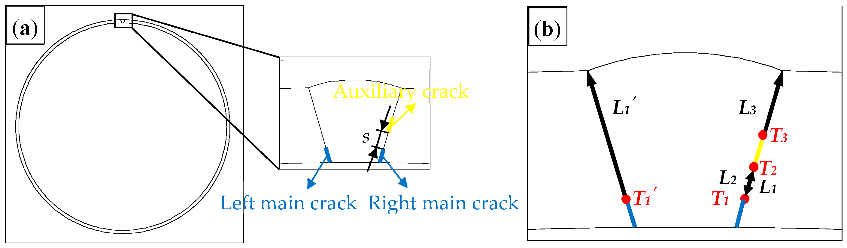
The double-crack model on the right side of Figure 1a consists of a main crack and an auxiliary crack. For comparative analysis, the left main crack model of the pipeline weld is established at the same position on the left side, which is symmetric with the right-hand side main crack. The blue line represents the main crack with the initial crack length l_m = 3 mm. The yellow line represents the auxiliary crack whose initial length is l_a = 3 mm. The initial distance between the right main crack tip and the right auxiliary crack tip (referring to the distance between the nodes near the two cracks) is denoted by s. We set the number of crack tips of the main and auxiliary cracks on the right as shown in Figure 1b: T₁, T₂, and T₃ represent crack tip 1, crack tip 2, and crack tip 3, L₁, L₂, and L₃ represent crack propagation path 1, path 2, and path 3, respectively. The crack tip of the left main crack used for comparison is represented by T₁’, and the propagation path is represented by L₁’.

2.2. The Finite Element Model

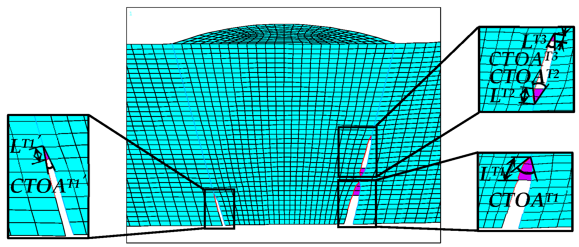
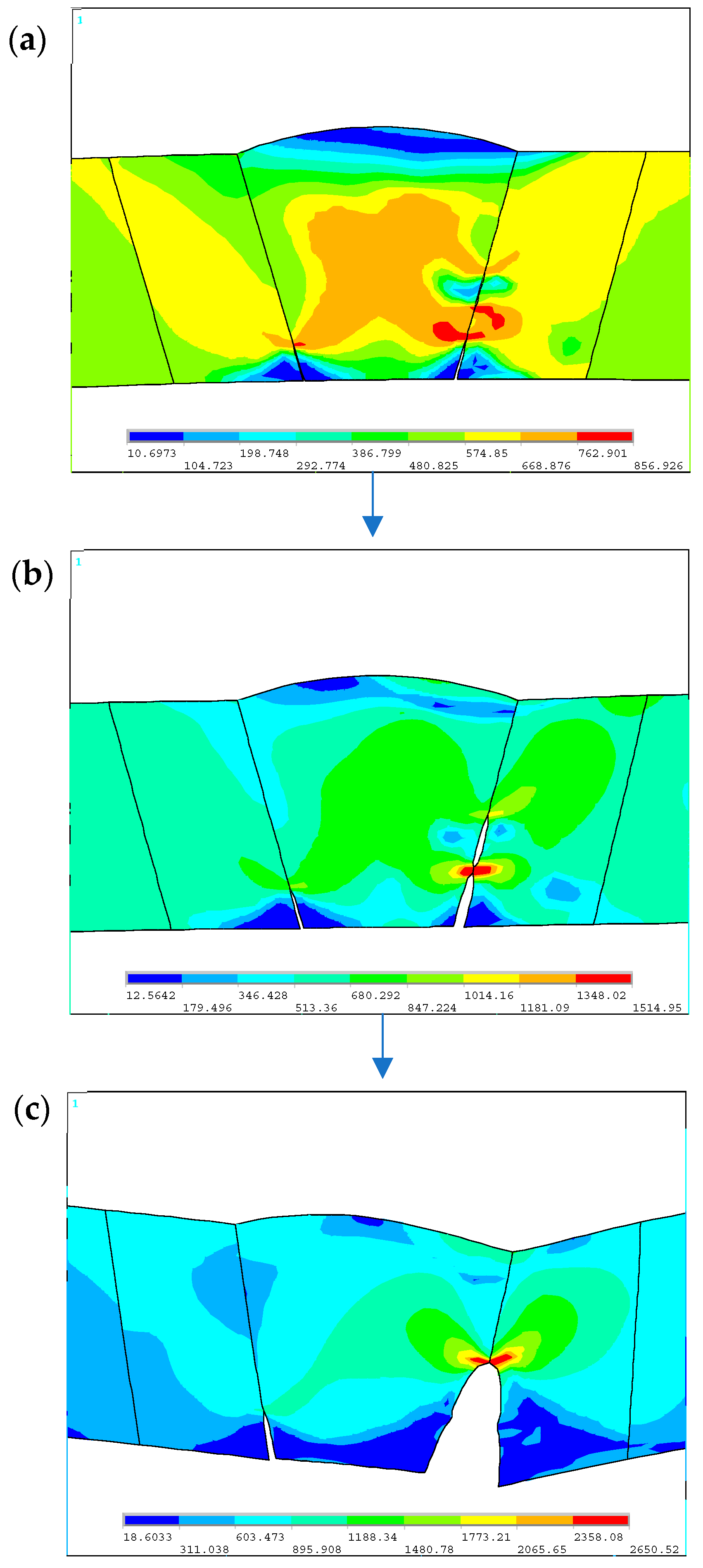
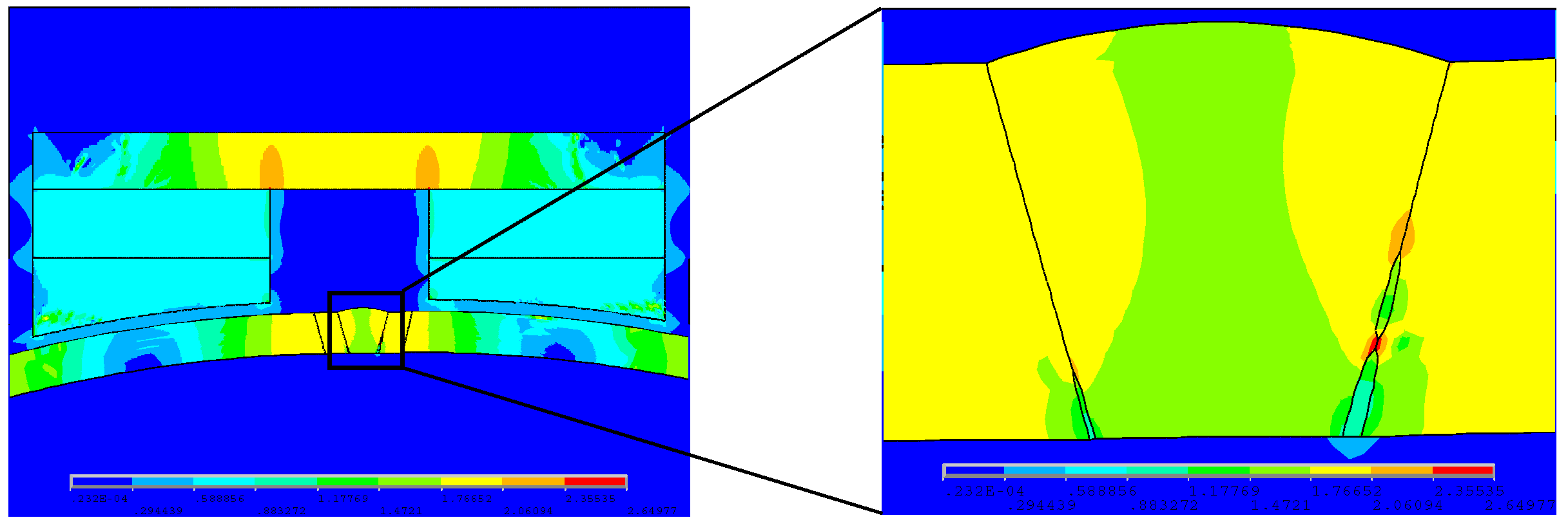
VCCT is used to cyclically calculate the energy release rate (G_I) of the type I crack tip at each load step. When G_I ≥ G_IC, the crack expands. The model established in this section has a discrete size of 0.5 mm on the crack propagation path. The expansion model of the certain load step in crack propagation is shown in Figure 2. The extension amount of the right main crack propagation path L₁ is represented by L^T1, and the extension amount of the left main crack propagation path L₁′ is represented by L^T1′. The CTOA of the main crack on the right is represented by CTOA^T1, the CTOA of the main crack on the left is represented by CTOA^T1′, and so on. Von-Mises stress patterns of the crack propagation process are shown in Figure 3. In Figure 3a, tip 1 of the main crack starts expanding; in Figure 3b, the main crack contacts the auxiliary crack, and in Figure 3c, the main crack merges with the auxiliary crack. It can be seen from Figure 3 that the peak value of Von-Mises stress is always at the crack tip and the driving force of the crack tip is the largest.

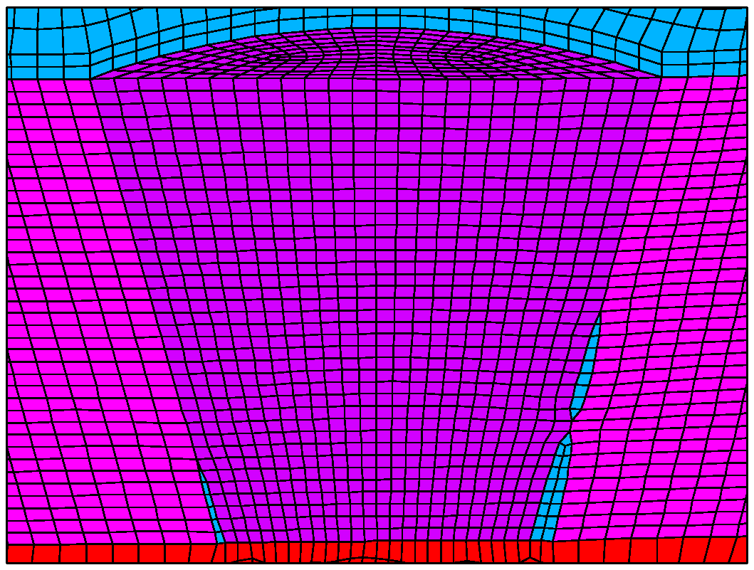
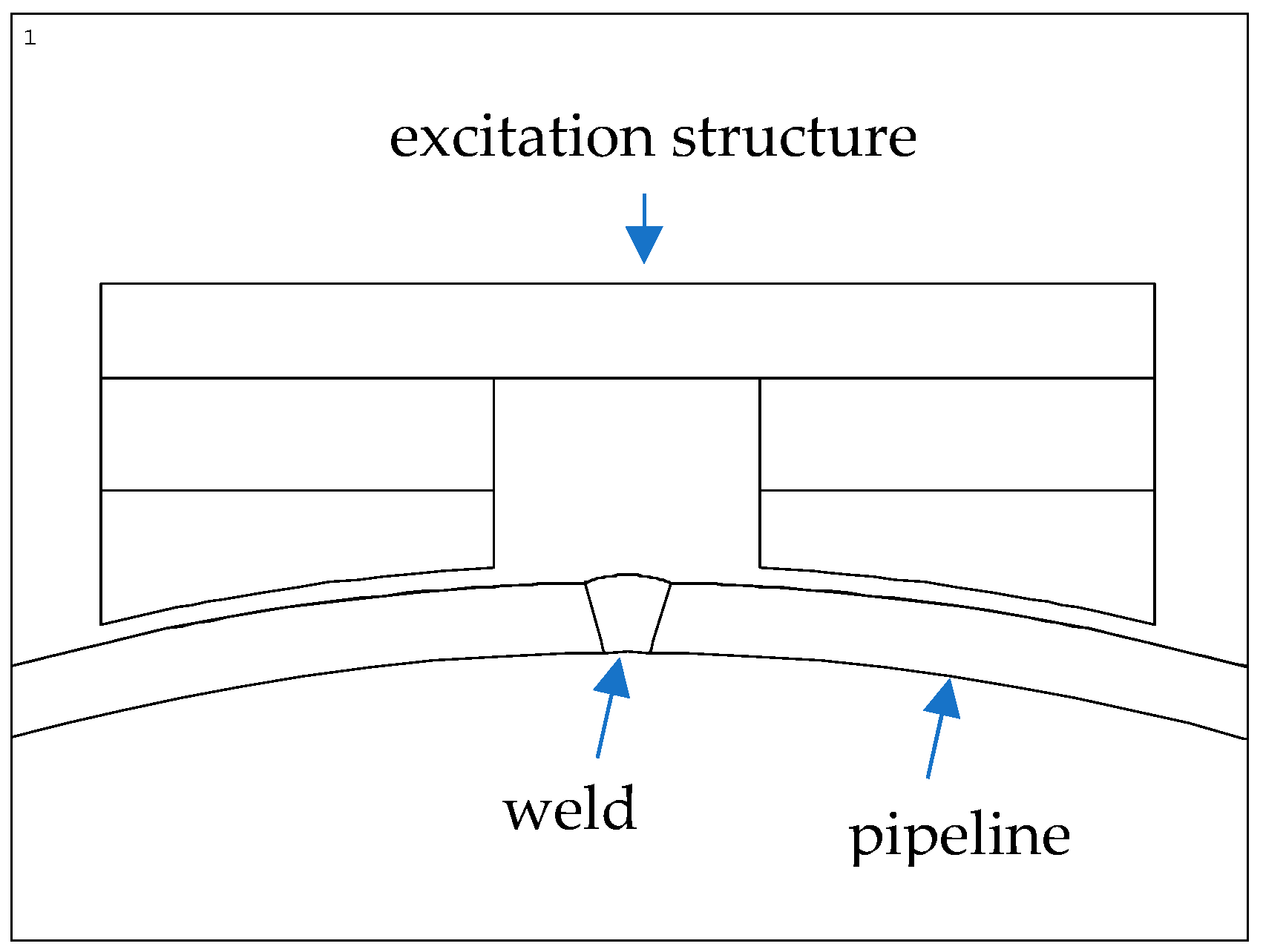
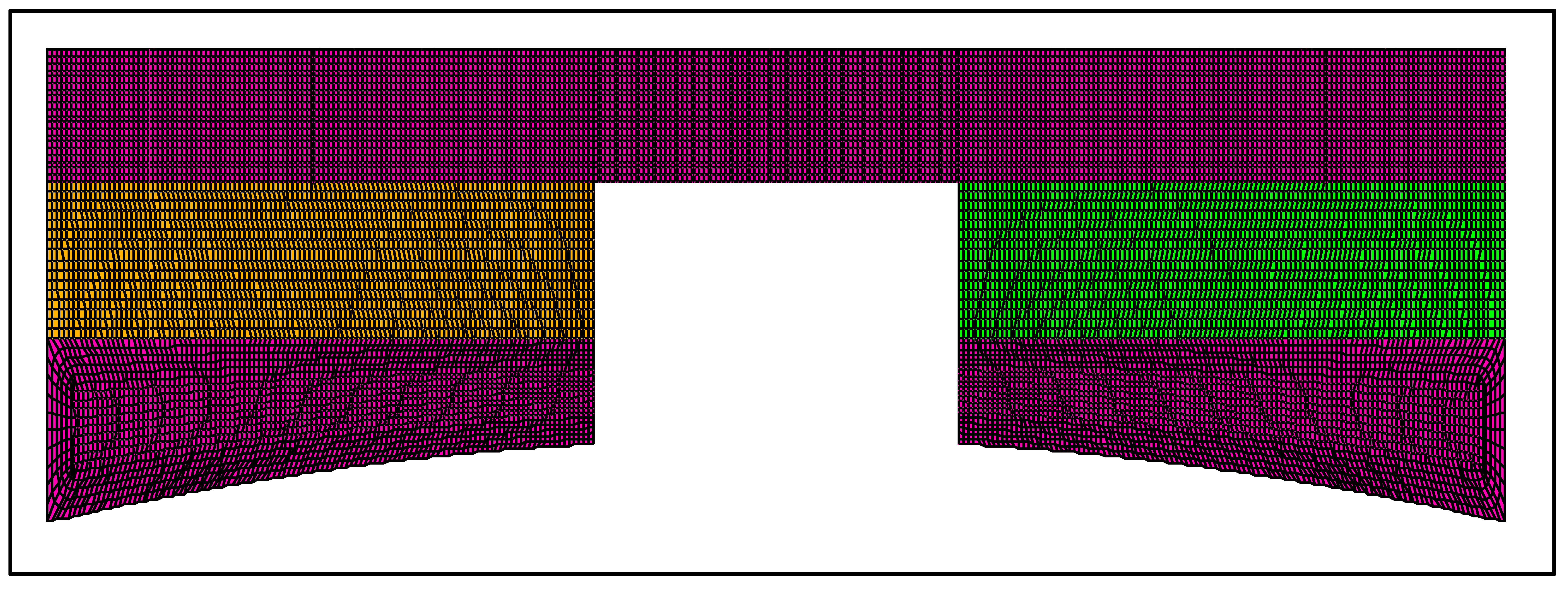
The computational domain around the multi-crack propagation is reconstructed, as shown in Figure 4. Each load step of crack propagation is accompanied by mesh re-division. The diagram of the pipeline weld and excitation structure is shown in Figure 5, and the sizes and material properties of the magnetized structure are shown in

Table 3. Magnetized structural dimensions and materials.

Dimensions	Materials
	magnet	Nd-Fe-B
	armature	armco iron
	pole shoe	armco iron

. The excitation structure model is shown in Figure 6. The MFL detection mechanism of pipeline welds can be found in previous studies [30,31] and the related literature [47,48,49].

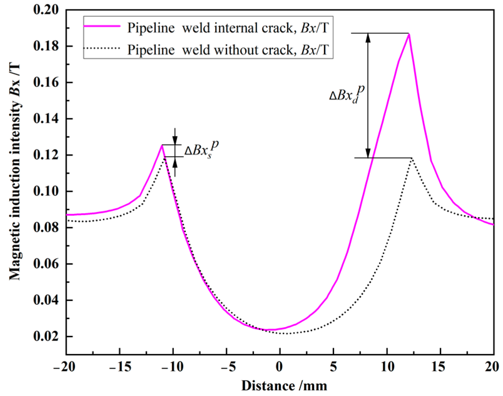
Crack propagation calculation and magnetic field analysis are carried out cyclically, and the magnetic induction intensity nephogram and magnetic induction intensity component curve under the certain load step are extracted, respectively, as shown in Figure 7 and Figure 8. Since there is no crack in the weld, a magnetic flux leakage signal will also be generated [30]; the model described has a single crack on the left and a double crack on the right. Therefore, the difference between the peak values of the magnetic induction intensity component of the single crack on the left side and the magnetic induction intensity component of the weld without cracks is set as $\Delta B{x}_s^p$. The difference between the peak values of the magnetic induction intensity component for the double crack (on the right side) and the magnetic induction intensity component of the weld without cracks is set as $\Delta B{x}_d^p$. The following characteristic quantities are extracted during the tip propagation process of the right main crack and the left main crack: the extended finite element number (EN), CTOA^T1 and CTOA^T1′, G_I^T1 and G_I^T1′ (G_I of the crack tip energy release rate of tip 1 of the right main crack is represented by G_I^T1, G_I of the crack tip energy release rate of tip 1 of the left main crack is represented by G_I^T1′), and $\Delta B{x}_d^p$ and $\Delta B{x}_s^p$. Several groups of the characteristic quantities in the crack propagation process are listed in

Table 4. Relevant feature quantities in the crack propagation process.

P (MPa)	GIT1 (N/mm)	GIT1′ (N/mm)	EN (Right Main Crack)	EN (Left Main Crack)	CTOAT1 (°)	CTOAT1′ (°)	$\Delta \mathit{B}{\mathit{x}}_{\mathit{d}}^{\mathit{p}}\left(\mathbf{T}\right)$	$\Delta \mathit{B}{\mathit{x}}_{\mathit{s}}^{\mathit{p}}\left(\mathbf{T}\right)$
18.6534	68.2124	60.0168	1	—	11.228	—	0.0231	0.0017
18.8034	189.6473	65.5480	2	—	23.778	—	0.0343	0.0047
18.8186	811.1834	80.5873	3	1	55.256	13.930	0.0681	0.0068

P—fluid pressure load, G_I^T1—crack tip energy release rate of tip 1 of the right main crack, G_I^T1′—crack tip energy release rate of tip 1 of the left main crack, EN—extended finite element number, and the discrete size of the element on the crack propagation path is 0.5 mm, CTOA^T1—crack tip opening angle of tip 1 of the right main crack, CTOA^T1′—crack tip opening angle of tip 1 of the left main crack, $\Delta B{x}_d^p$—difference between the peak values of the magnetic induction intensity component for the double crack (on the right side) and the magnetic induction intensity component of the weld without cracks, $\Delta B{x}_s^p$—difference between the peak values of the magnetic induction intensity component of the single crack on the left side and the magnetic induction intensity component of the weld without cracks.

.

It can be seen from Table 4 that when the fluid pressure load P = 18.6534 MPa, the main crack on the right side starts to propagate, and the main crack on the left side does not propagate until P = 18.8186 MPa. At this moment, the main crack on the right side has expanded by 3 EN. Under the loads of 18.6534 and 18.8034 MPa, the left main crack does not propagate, and CTOA^T1′ is not extracted. The crack initiation pressure of the right main crack is smaller than that of the left main crack. Under the same pressure load, the crack tip energy release rate of the right main crack is larger, and the driving force for the propagate is stronger, which results in a larger CTOA^T1. During the crack propagation, the severe deformation of the pipeline weld structure affects the distribution of the pipeline weld magnetic field, resulting in an increase of the magnetic induction intensity component, which, in turn, results in $\Delta B{x}_d^p$ being larger than $\Delta B{x}_s^p$. For example, when P = 18.8186 MPa, $\Delta B{x}_d^p:\Delta B{x}_s^p=0.0681:0.0068\cong 10.01:1$. The obtained results indicate the interference effect of the auxiliary crack on the right main crack accelerates the propagation of the right main crack.

3. Crack Tip Distance and Size Effect

3.1. Crack Tip Distance Effect

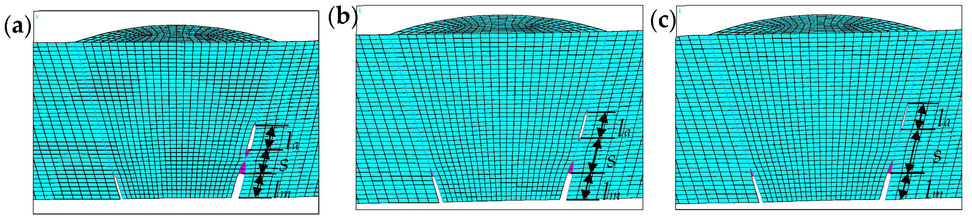
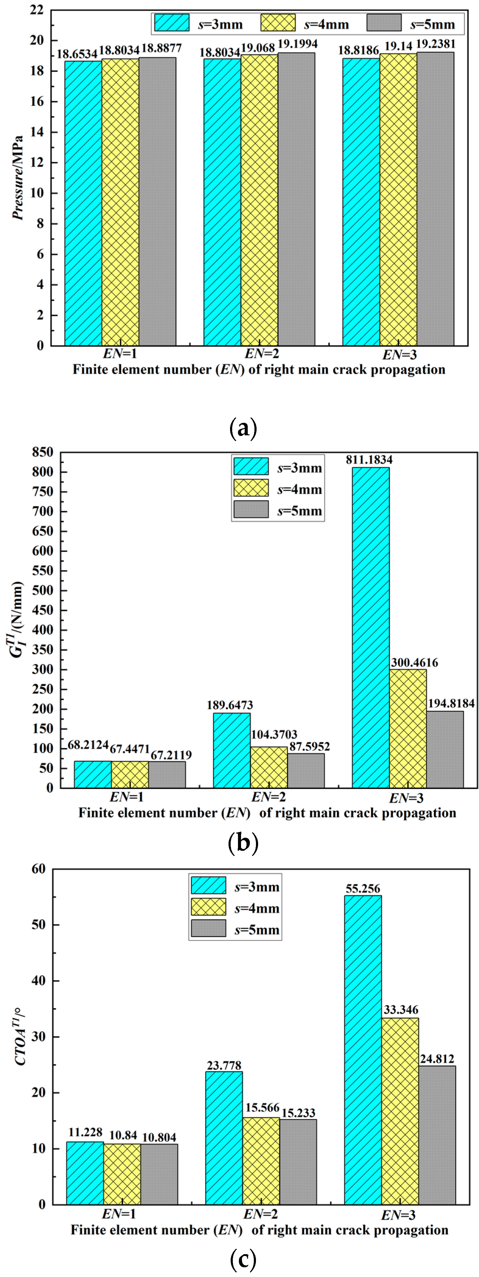
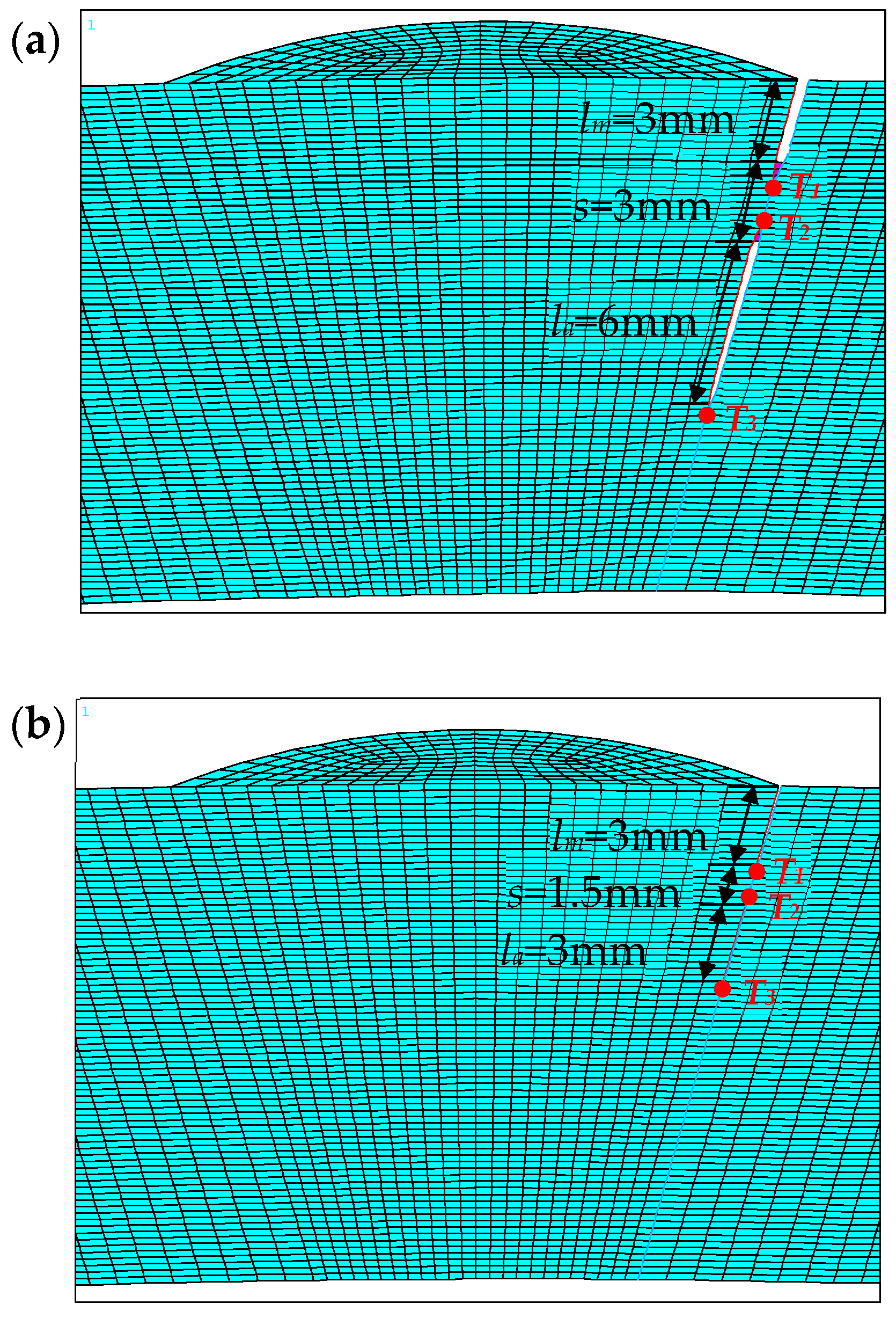
To analyze the influence of the crack tip distance between the auxiliary crack and the main crack, l_m is set to 3 mm, l_a is set to 3 mm, s is set to 3, 4, and 5 mm, respectively. The crack propagation at a certain load step is extracted, as shown in Figure 9. The model established in this section has a discrete size of 0.5 mm on the crack propagation path. By extracting the crack propagation results of each load step, the node coordinates are updated according to the deformation, and the computation grid around the crack position is reconstructed. Fatigue crack propagation calculation and magnetic field analysis are performed cyclically, and the characteristic quantities of the right main crack are extracted, including EN, CTOA^T1, G_I^T1, and $\Delta B{x}_d^p$. They are all listed in

Table 5. Interference effect of crack tip distance on main crack.

EN (Right Main Crack)	s (mm)	P (MPa)	GIT1 (N/mm)	CTOAT1 (°)	$\Delta \mathit{B}{\mathit{x}}_{\mathit{d}}^{\mathit{p}}\left(\mathbf{T}\right)$
1	3	18.6534	68.2124	11.228	0.0231
	4	18.8034	67.4471	10.84	0.0230
	5	18.8877	67.2119	10.804	0.0227
2	3	18.8034	189.6473	23.778	0.0343
	4	19.068	104.3703	15.566	0.0339
	5	19.1994	87.5952	15.233	0.0335
3	3	18.8186	811.1834	55.256	0.0681
	4	19.14	300.4616	33.346	0.0489
	5	19.2381	194.8184	24.812	0.0436

EN—extended finite element number, and the discrete size of the element on the crack propagation path is 0.5 mm, s—initial distance between the right main crack tip and the right auxiliary crack tip, P—fluid pressure load, G_I^T1—crack tip energy release rate of tip 1 of the right main crack, CTOA^T1—crack tip opening angle of tip 1 of the right main crack, $\Delta B{x}_d^p$—difference between the peak values of the magnetic induction intensity component for the double crack (on the right side) and the magnetic induction intensity component of the weld without cracks.

. When the EN of the main crack on the right side is 1, 2, or 3, the variation law P-s of the fluid pressure load inside the pipeline with the distance from the crack tip is shown in Figure 10a; the variation law G_I^T1-s of the energy release rate of T₁ of the main crack on the right side with the distance from the crack tip is shown in Figure 10b; the variation law CTOA^T1-s of the crack tip opening angle of the main crack on the right side with the distance from the crack tip is shown in Figure 10c; the variation law of $\Delta B{x}_d^p$ with the distance from the crack tip is shown in Figure 10d.

It can be seen from Table 5 and Figure 10 that when the distance s from the crack tip changes, the characteristic quantities of the crack propagation process can be obtained as follows:

(1) s = 3 mm, crack propagation pressure P = 18.6534 MPa; s = 4 mm, crack propagation pressure P = 18.8034 MPa; s = 5 mm, crack propagation pressure P = 18.8877 MPa. From s= 3 mm to s = 4 mm to s = 5 mm, the crack propagation pressure is getting bigger and bigger.

(2) From s = 3 mm to s = 4 mm to s = 5 mm, when expanding the same number of finite elements (EN = 1 or EN = 2 or EN = 3), G_I^T1, CTOA^T1, and $\Delta B{x}_d^p$ are getting smaller and smaller. Taking EN = 3 as an example, the ratio of the peak value $\Delta B{x}_d^p$ of the three cases is $0.0681:0.0489:0.0436\cong 1.56:1.12:1$.

From the above characteristics, it can be found that as the distance s between the auxiliary crack and the main crack tips increases, the crack propagation pressure becomes larger and larger, indicating that the main crack is not likely to propagate. The calculated value of G_I^T1 decreases and the driving force for crack propagation decreases, resulting in CTOA^T1 becoming smaller and smaller, and the deformation of the pipeline weld structure decreases, which affects the pipeline weld magnetic field distribution during the crack propagation process, the detected $\Delta B{x}_d^p$. shows a decreasing trend with an increasing crack tip distance s. Therefore, it will become more and more dangerous when the crack tip distance s is getting shorter.

3.2. Influence of the Auxiliary Crack Size on Main Crack

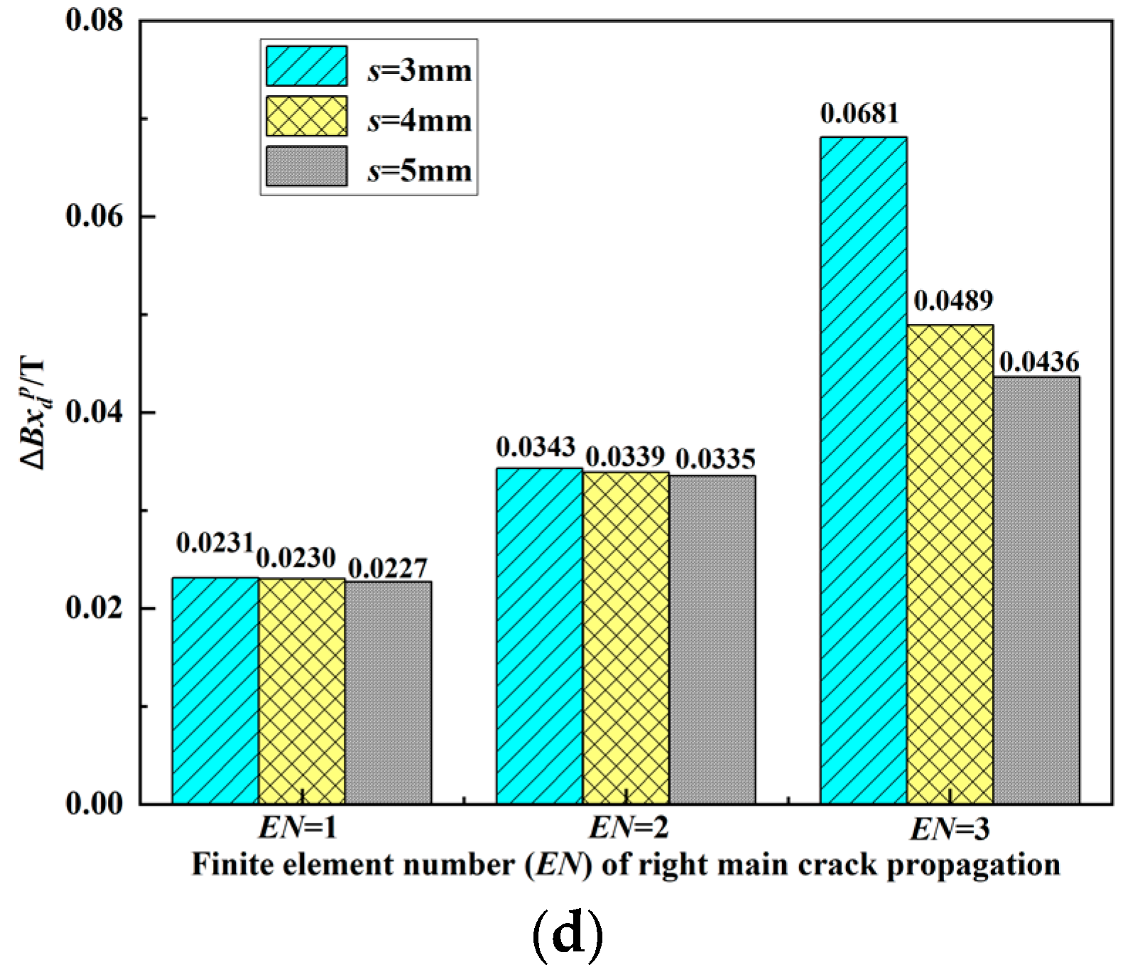
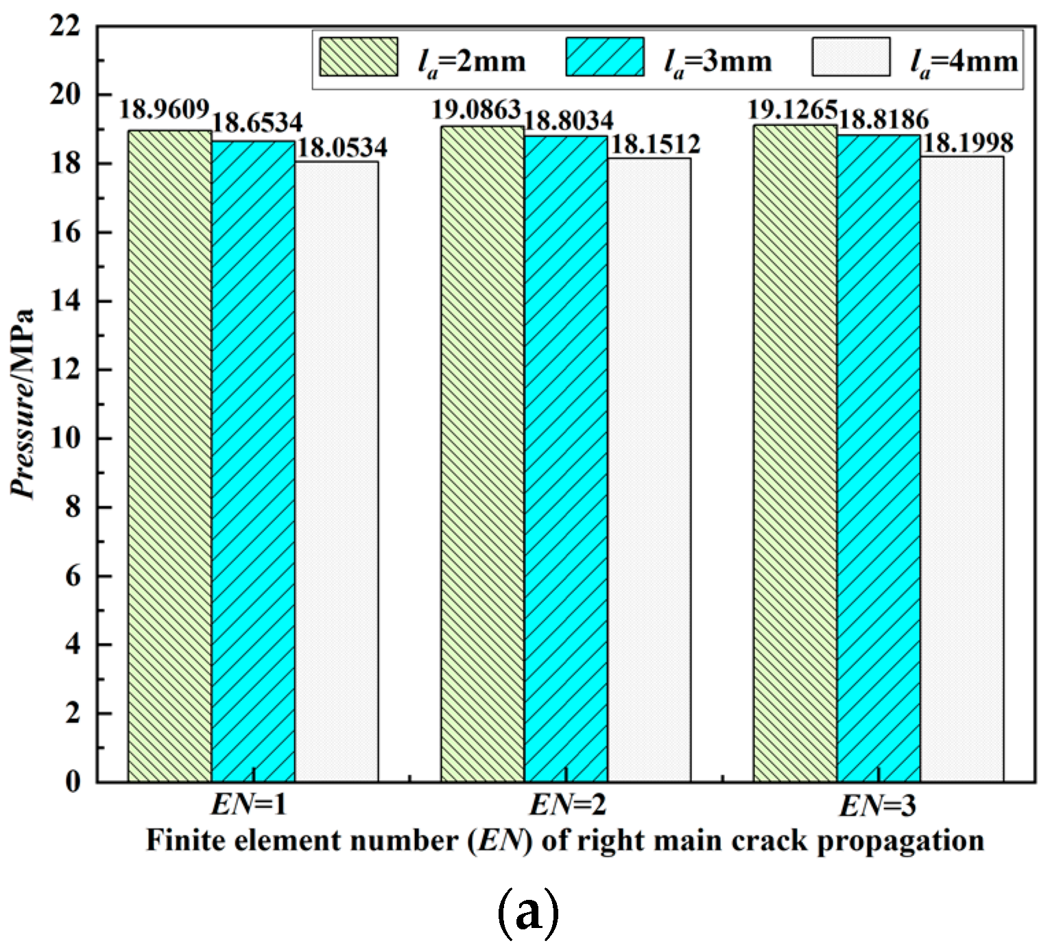
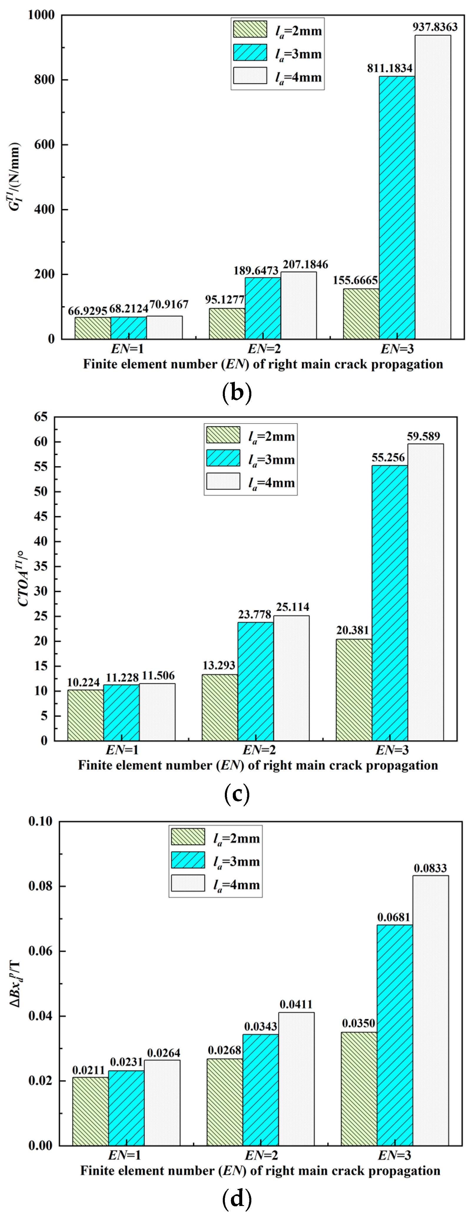
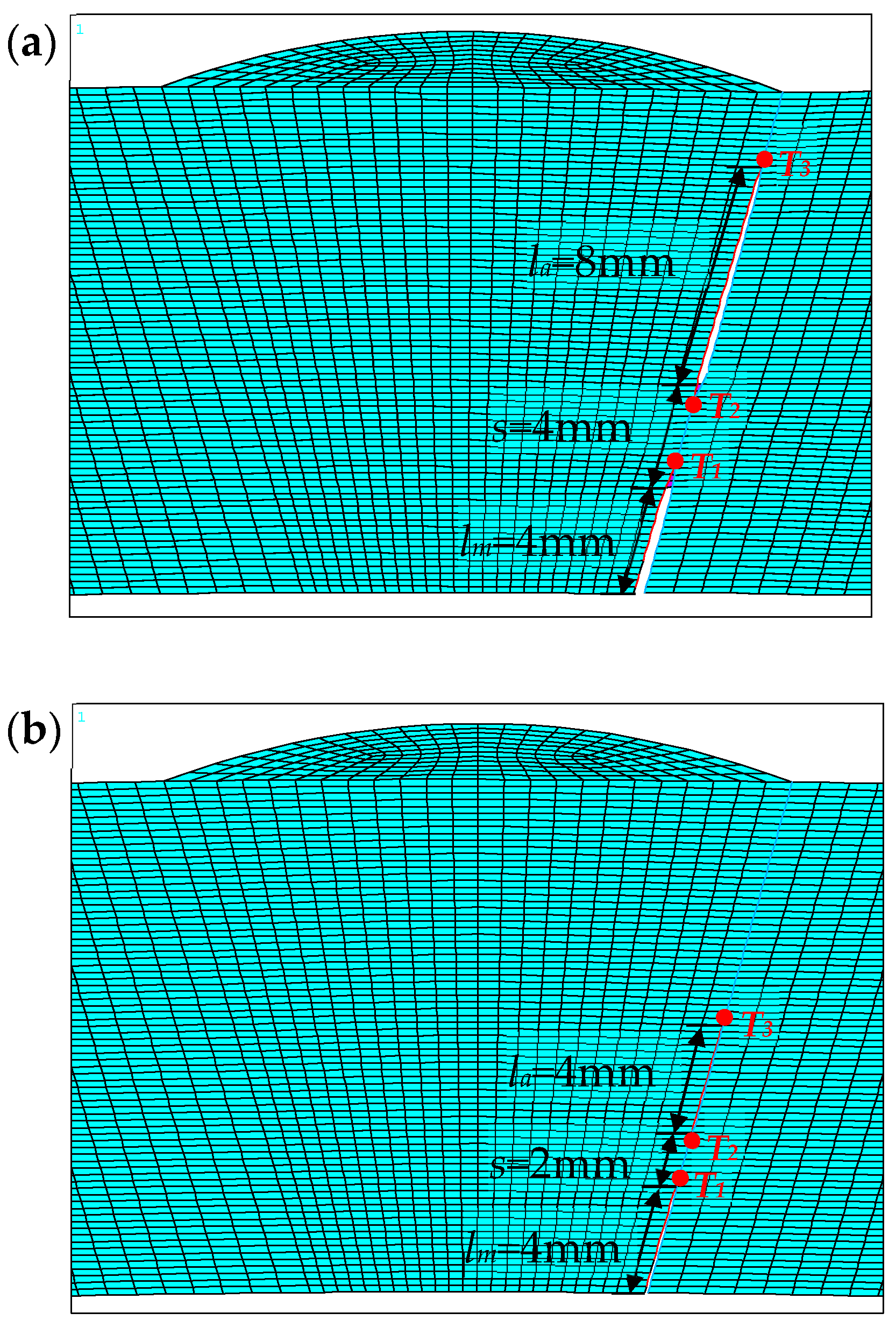
To analyze the effect of the auxiliary crack size on the main crack, l_m is set to 3 mm, s is set to 3 mm, l_a is set to 2, 3, and 4 mm, respectively. The crack propagation process at certain load steps is shown in Figure 11. At each load step, the node coordinates are updated according to the deformation, and the calculation grid around the crack position is reconstructed. Crack propagation calculation and magnetic field analysis are performed cyclically, and the main characteristic quantities are extracted, including EN, CTOA^T1, G_I^T1, and $\Delta B{x}_d^p$. They are all listed in

Table 6. Influence of the auxiliary crack size.

EN (Right Main Crack)	la (mm)	P (MPa)	GIT1 (N/mm)	CTOAT1 (°)	$\Delta \mathit{B}{\mathit{x}}_{\mathit{d}}^{\mathit{p}}\left(\mathbf{T}\right)$
1	2	18.9609	66.9295	10.224	0.0211
	3	18.6534	68.2124	11.228	0.0231
	4	18.0534	70.9167	11.506	0.0264
2	2	19.0863	95.1277	13.293	0.0268
	3	18.8034	189.6473	23.778	0.0343
	4	18.1512	207.1846	25.114	0.0411
3	2	19.1265	155.6665	20.381	0.0350
	3	18.8186	811.1834	55.256	0.0681
	4	18.1998	937.8363	59.589	0.0833

EN—extended finite element number, and the discrete size of the element on the crack propagation path is 0.5 mm, l_a—initial length of the auxiliary crack, P—fluid pressure load, G_I^T1—crack tip energy release rate of tip 1 of the right main crack, CTOA^T1—crack tip opening angle of tip 1 of the right main crack, $\Delta B{x}_d^p$—difference between the peak values of the magnetic induction intensity component for the double crack (on the right side) and the magnetic induction intensity component of the weld without cracks.

. When the value of EN of the main crack on the right side is 1, 2, or 3, the variation law P-l_a of the fluid pressure load inside the pipeline with the initial length of the auxiliary crack is shown in Figure 12a. The variation law G_I^T1-l_a of the energy release rate of T₁ of the main crack on the right side with the initial length of the auxiliary crack is shown in Figure 12b. The variation law CTOA^T1-l_a of the opening angle of the main crack on the right side with the initial length of the auxiliary crack is shown in Figure 12c; the variation law $\Delta B{x}_d^p$-l_a of the peak value difference varying with the initial length of the auxiliary crack is shown in Figure 12d.

From Table 6 and Figure 12, when the auxiliary crack size la changes, the characteristics of the crack propagation process are given as follows:

(1) When l_a = 2 mm, the crack propagation pressure P = 18.9609 MPa; l_a = 3 mm, the crack propagation pressure P = 18.6534 MPa; l_a = 4 mm, the crack propagation pressure P = 18.0534 MPa. From l_a = 2 mm to l_a = 3 mm to l_a = 4 mm, the crack propagation pressure needed decreases.

(2) From l_a = 2 mm to l_a = 3 mm to l_a = 4 mm, when the same number of finite elements is expanded (EN =1 or EN =2 or EN =3), G_I^T1, CTOA^T1, and $\Delta B{x}_d^p$ all keep increasing. Taking EN = 3 as an example, the ratio of the peak value $\Delta B{x}_d^p$ of the three cases is $0.0350:0.0681:0.0833\cong 1:1.95:2.38$.

From the above characteristics, it can be found that with the increasing auxiliary crack size l_a, the crack propagation pressure becomes smaller and smaller, indicating that the main crack becomes easier to expand. When expanding the same number of finite elements, G_I^T1 becomes larger and larger, and the driving force of crack propagation increases, which leads to the increase of CTOA^T1. The deformation increase of the pipeline weld affects the distribution of the pipeline weld’s magnetic field during the crack propagation. The detected $\Delta B{x}_d^p$ shows an increasing trend with the increase of the auxiliary crack size l_a. Therefore, with the increasing auxiliary crack size, the interference effect is more intensified. The crack interaction makes the failure easier to occur.

4. Comparative Analysis

Through the analysis in the second subsection, it is seen that the existence of auxiliary cracks enhances the propagation danger of the main crack. Through the analysis in the third subsection, it is seen that the enhancement effect of the auxiliary crack on the main crack increases with the increasing auxiliary crack size and decreases with the distance between the auxiliary the main crack tips. In order to measure the strength of the dynamic interference effect caused by these two factors, we comprehensively analyze the change law of the characteristic quantities in the crack propagation process under the combined action of these two factors. For statement convenience, two parameters, ${\gamma }_l$ and ${\gamma }_s$, are introduced, here ${\gamma }_l$ is the ratio of the initial length of the main crack l_m to the initial length of the auxiliary crack l_a, and ${\gamma }_s$ is the ratio of the crack tip distance s to the initial length of the main crack l_m:

$${\gamma }_l=\frac{l_m}{l_a}$$

(1)

$${\gamma }_s=\frac{s}{l_m}$$

(2)

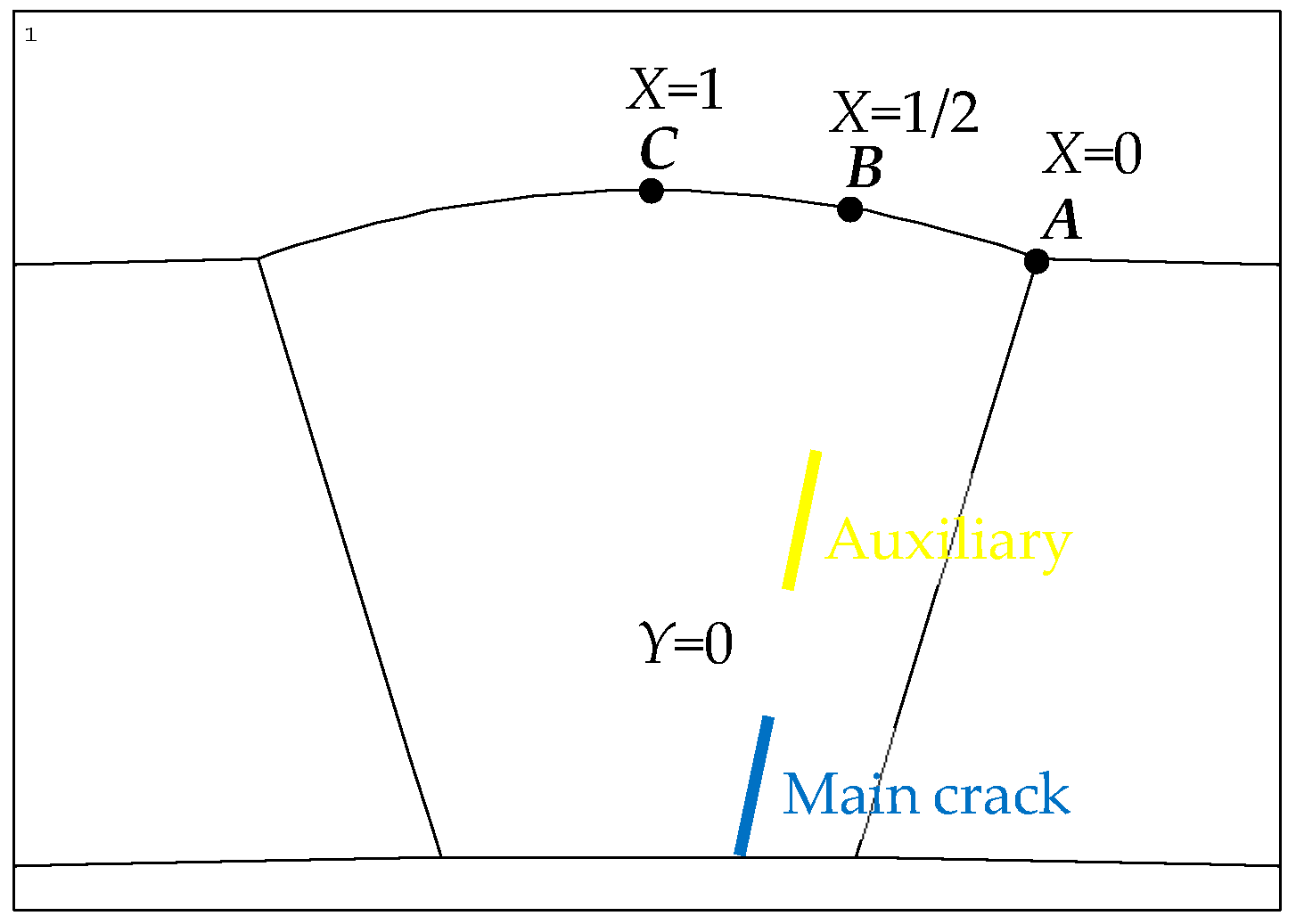
Since multiple cracks can be distributed on the outer wall of the weld, the inside of the weld, and the inner wall of the weld, models of multiple cracks in different radial directions of the pipeline weld were established. In order to verify the universality of this method, in addition to considering the cracks in the fusion zone, a multi-crack model was also established at the position of half the arc length from the fusion zone to the center of the weld bead. (This section has only one main crack and one subsidiary crack established on the right-hand side). As shown in Figure 13, points A and C are, respectively, set at the left and right ends of the weld zone, and point B is set at the center of the weld bead. Setting the double crack at the circumferential position X of the pipe weld is represented as follows: X = 0 represents the distribution of cracks at the position of the fusion zone; X = 1/2 represents the distribution of cracks at the position of 1/2 arc length (arc length of AB) from the fusion zone to the center of the weld bead; X = 1 represents the distribution of cracks at the center of the weld bead. Setting the double crack at the radial position of the pipeline weld is represented as follows: Y = 0 denotes that the main crack is the inner wall crack, and the auxiliary crack is the internal crack of the pipeline weld; Y = 1 denotes that the main crack is the outer wall crack, and the auxiliary crack is the internal crack of the pipeline weld. Figure 13 is a schematic diagram of the X = 1/2, Y = 0 model.

Three sets of numerical examples are established. Each example analyzes the multi-crack interaction by keeping the initial size of l_m, circumferential position (X), and radial position (Y) unchanged.

The first set of calculation examples follows:

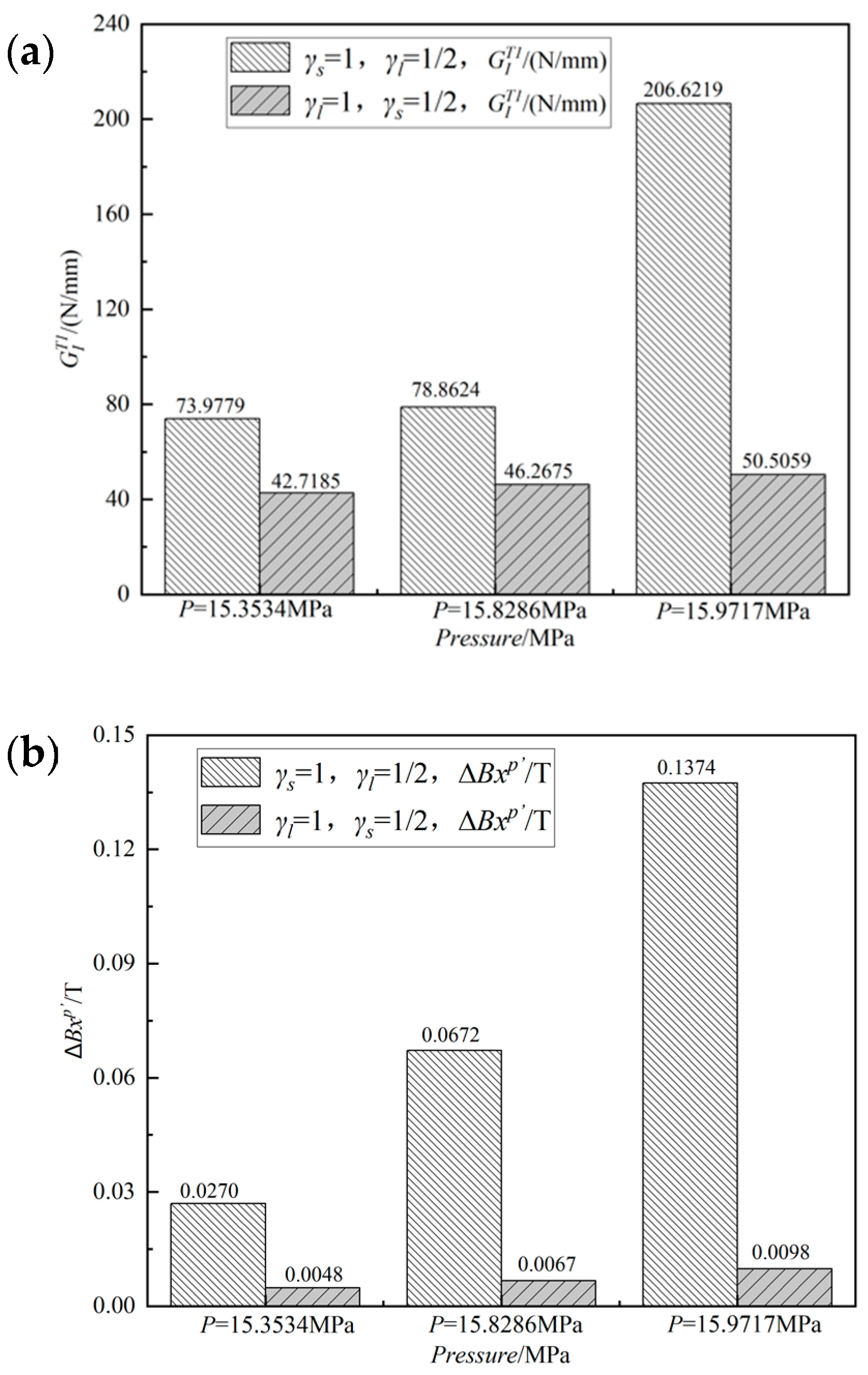
$\{\begin{array}{c}{l}_m=3 \mathrm{mm}\\ X=0,Y=1\\ {\gamma }_s=1,{\gamma }_l=\frac{1}{2}\end{array}$ and $\{\begin{array}{c}{l}_m=3 \mathrm{mm}\\ X=0,Y=1\\ {\gamma }_l=1,{\gamma }_s=\frac{1}{2}\end{array}$, P = 15.9717 MPa, the crack propagation process is shown in Figure 14.

The second set of calculation examples follows:

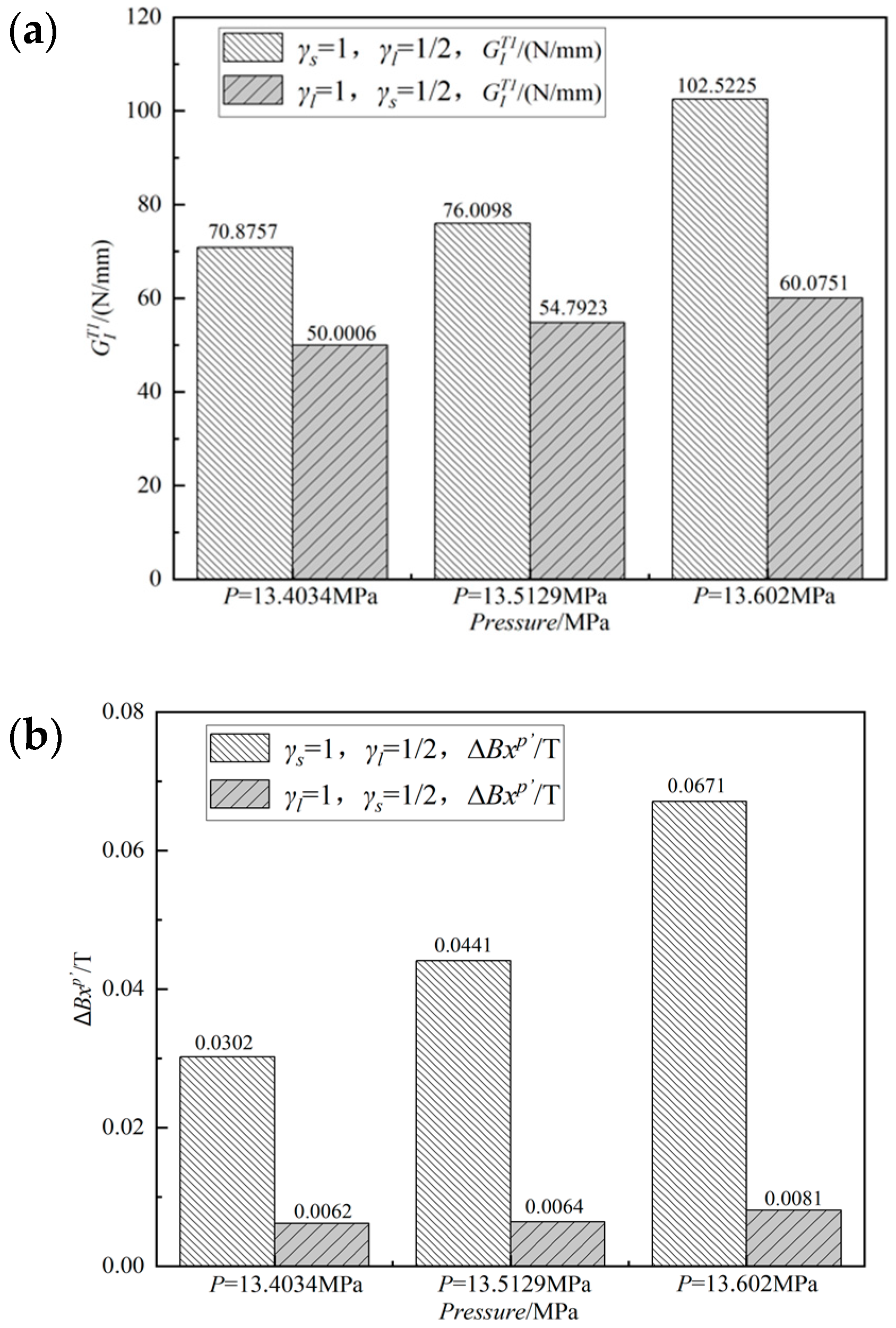
$\{\begin{array}{c}{l}_m=4 \mathrm{mm}\\ X=0,Y=0\\ {\gamma }_s=1,{\gamma }_l=\frac{1}{2}\end{array}$ and $\{\begin{array}{c}{l}_m=4 \mathrm{mm}\\ X=0,Y=0\\ {\gamma }_l=1,{\gamma }_s=\frac{1}{2}\end{array}$, P = 13.602 MPa, the crack propagation process is shown in Figure 15.

The third set of calculation examples follows:

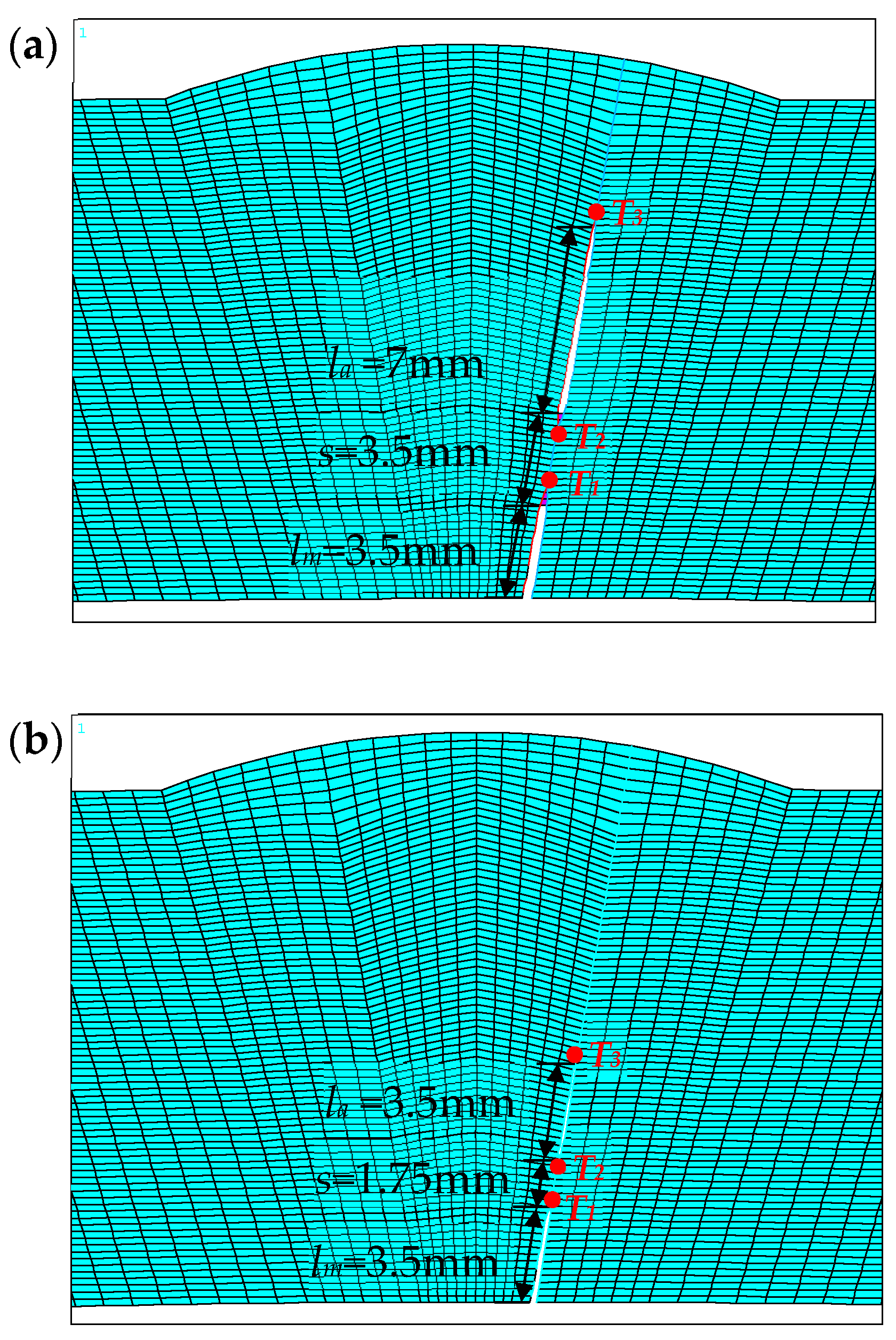
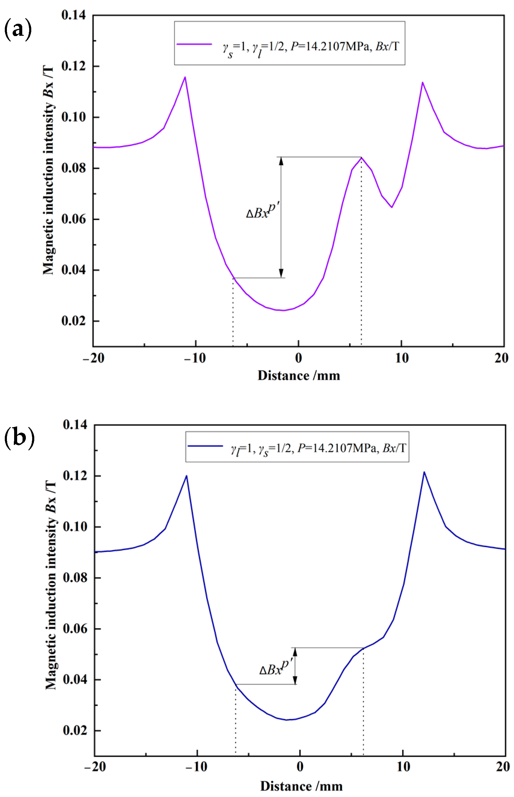
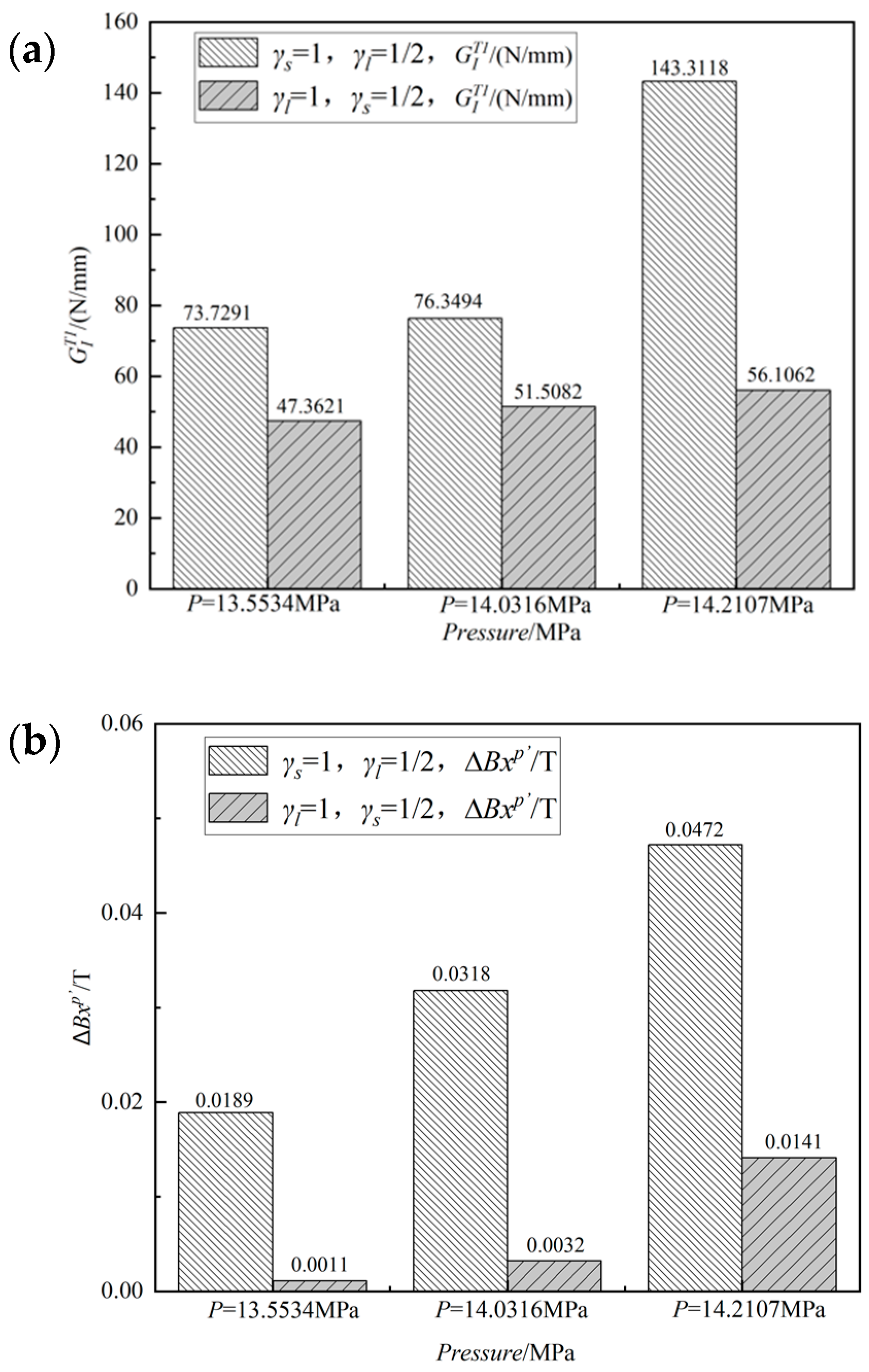
$\{\begin{array}{c}{l}_m=3.5 \mathrm{mm}\\ X=\frac{1}{2},Y=0\\ {\gamma }_s=1,{\gamma }_l=\frac{1}{2}\end{array}$ and $\{\begin{array}{c}{l}_m=3.5 \mathrm{mm}\\ X=\frac{1}{2},Y=0\\ {\gamma }_l=1,{\gamma }_s=\frac{1}{2}\end{array}$, P = 14.2107 MPa, the crack propagation process is shown in Figure 16. In this section, the discrete size of the element on the crack propagation path is 0.25 mm. The main crack tip (T₁) and the auxiliary crack tips (T₂ and T₃) of three sets of numerical examples are shown in Figure 14, Figure 15 and Figure 16, respectively.

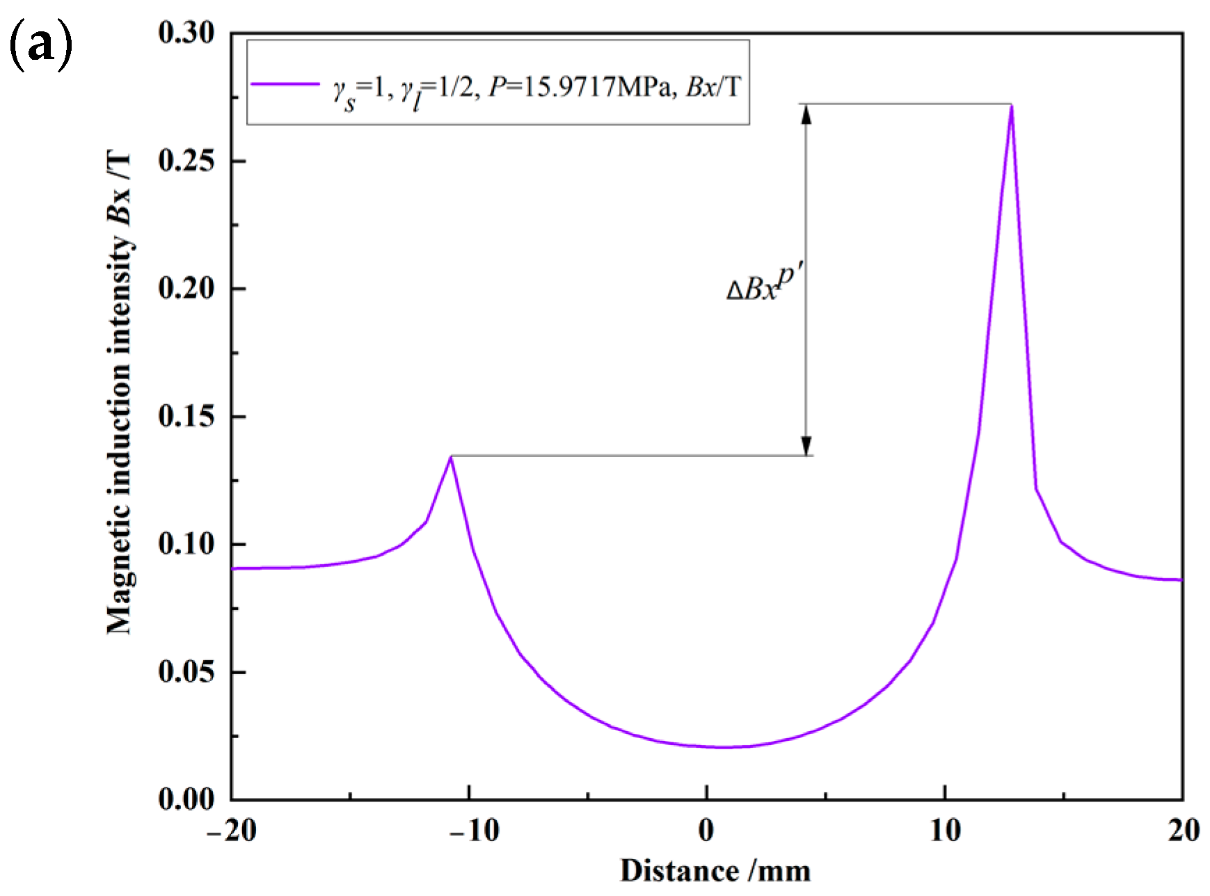
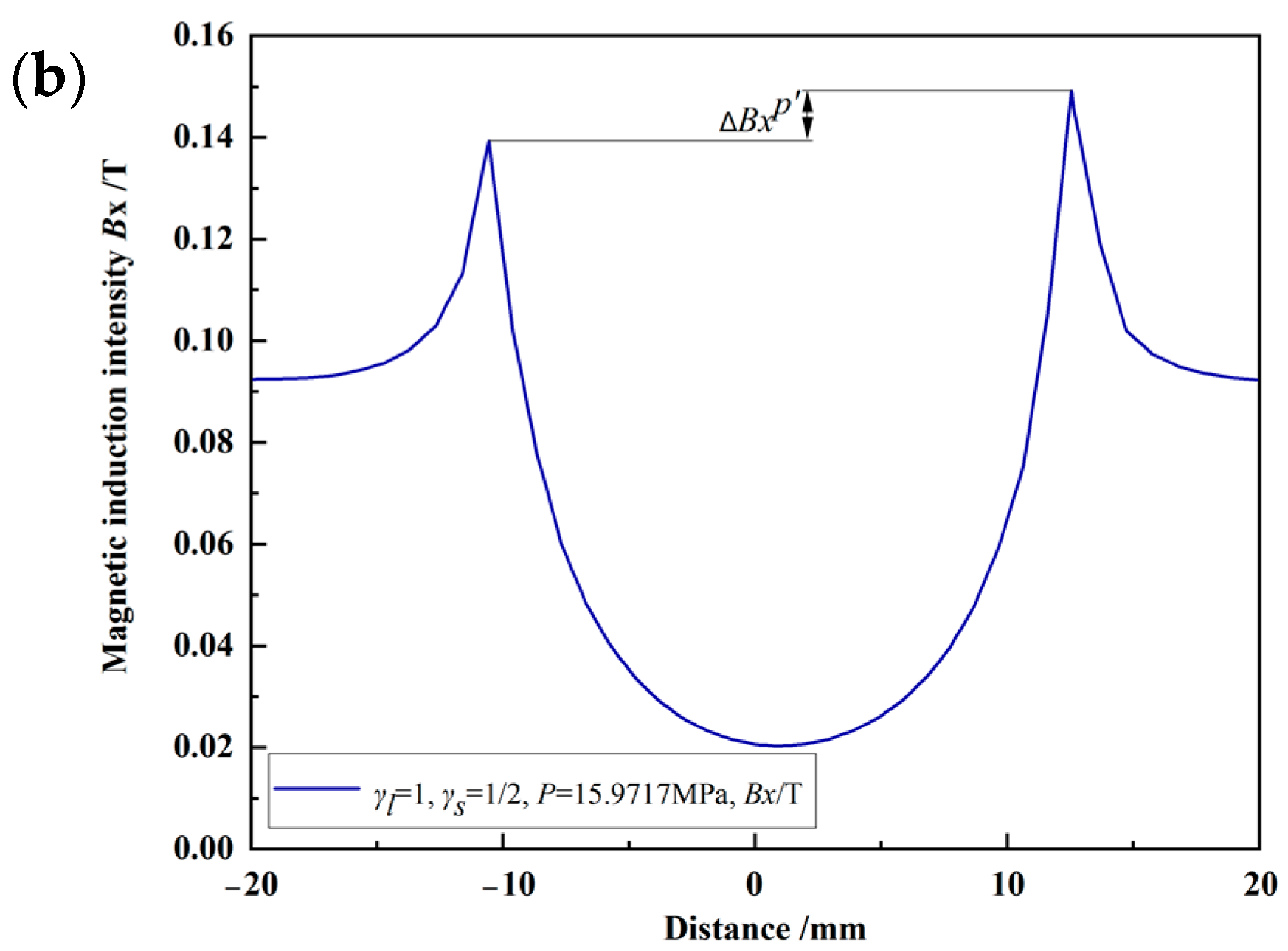
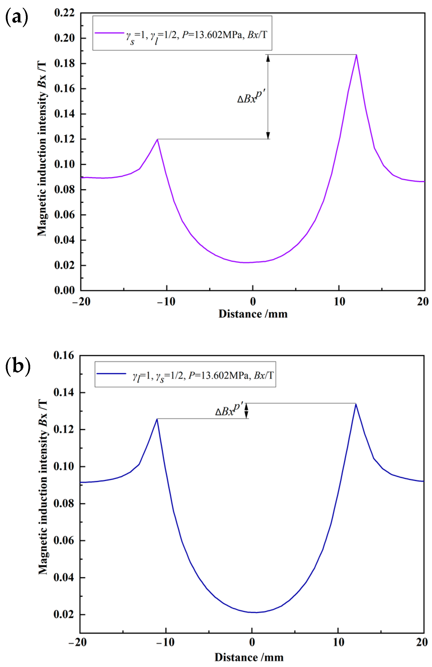
The crack propagation calculation and magnetic field analysis are performed cyclically for each group of examples, and the characteristic quantities in the crack tip propagation process of the main crack are extracted: the extended finite element number EN’ (in this section, it is denoted as EN’ to distinguish it from the previous two sections), CTOA^T1, G_I^T1, and the peak values difference $\Delta B{x}^{p^{\prime }}$ are shown in

Table 7. Changes of the interference parameters ${\gamma }_l$ and ${\gamma }_s$ for the first set of the simulation examples.

P (MPa)	EN’	GIT1 (N/mm)	CTOAT1 (°)	$$\Delta \mathit{B}{\mathit{x}}^{\mathit{p}\prime }\left(\mathbf{T}\right)$$
15.3534	$${\gamma }_s=1, {\gamma }_l=\frac{1}{2}$$ : 1 EN′	${\gamma }_s=1, {\gamma }_l=\frac{1}{2}$: 73.9779	${\gamma }_s=1, {\gamma }_l=\frac{1}{2}$: 11.942	${\gamma }_s=1, {\gamma }_l=\frac{1}{2}$: 0.0270
	${\gamma }_l=1, {\gamma }_s=\frac{1}{2}$: 0	${\gamma }_l=1, {\gamma }_s=\frac{1}{2}$: 42.7185	${\gamma }_l=1, {\gamma }_s=\frac{1}{2}$: —	${\gamma }_l=1, {\gamma }_s=\frac{1}{2}$: 0.0048
15.8286	${\gamma }_s=1, {\gamma }_l=\frac{1}{2}$: 2 EN′	${\gamma }_s=1, {\gamma }_l=\frac{1}{2}$: 78.8624	${\gamma }_s=1, {\gamma }_l=\frac{1}{2}$: 18.305	${\gamma }_s=1, {\gamma }_l=\frac{1}{2}$: 0.0672
	${\gamma }_l=1, {\gamma }_s=\frac{1}{2}$: 0	${\gamma }_l=1, {\gamma }_s=\frac{1}{2}$: 46.2675	${\gamma }_l=1, {\gamma }_s=\frac{1}{2}$: —	${\gamma }_l=1, {\gamma }_s=\frac{1}{2}$: 0.0067
15.9717	${\gamma }_s=1, {\gamma }_l=\frac{1}{2}$: 3 EN′	${\gamma }_s=1, {\gamma }_l=\frac{1}{2}$: 206.6219	${\gamma }_s=1, {\gamma }_l=\frac{1}{2}$: 36.955	${\gamma }_s=1, {\gamma }_l=\frac{1}{2}$: 0.1374
	${\gamma }_l=1, {\gamma }_s=\frac{1}{2}$: 0	${\gamma }_l=1, {\gamma }_s=\frac{1}{2}$: 50.5059	${\gamma }_l=1, {\gamma }_s=\frac{1}{2}$: —	${\gamma }_l=1, {\gamma }_s=\frac{1}{2}$: 0.0098

P—fluid pressure load, EN′—extended finite element number, and the discrete size of the element on the crack propagation path is 0.25 mm, G_I^T1—crack tip energy release rate of tip 1 of the right main crack, CTOA^T1—crack tip opening angle of tip 1 of the right main crack, $\Delta B{x}^{p^{\prime }}$—difference between the peak value of the magnetic induction intensity component at the crack and the magnetic induction intensity component of its symmetrical position.

,

Table 8. Changes of the interference parameters ${\gamma }_l$ and ${\gamma }_s$ for the second set of the simulation examples.

P (MPa)	EN’	GIT1 (N/mm)	CTOAT1 (°)	$$\Delta \mathit{B}{\mathit{x}}^{\mathit{p}\prime }\left(\mathbf{T}\right)$$
13.4034	$${\gamma }_s=1, {\gamma }_l=\frac{1}{2}$$ : 1 EN′	${\gamma }_s=1, {\gamma }_l=\frac{1}{2}$: 70.8757	${\gamma }_s=1, {\gamma }_l=\frac{1}{2}$: 12.279	${\gamma }_s=1, {\gamma }_l=\frac{1}{2}$: 0.0302
	${\gamma }_l=1, {\gamma }_s=\frac{1}{2}$: 0	${\gamma }_l=1, {\gamma }_s=\frac{1}{2}$: 50.0006	${\gamma }_l=1, {\gamma }_s=\frac{1}{2}$: —	${\gamma }_l=1, {\gamma }_s=\frac{1}{2}$: 0.0062
13.5129	${\gamma }_s=1, {\gamma }_l=\frac{1}{2}$: 2 EN′	${\gamma }_s=1, {\gamma }_l=\frac{1}{2}$: 76.0098	${\gamma }_s=1, {\gamma }_l=\frac{1}{2}$: 15.372	${\gamma }_s=1, {\gamma }_l=\frac{1}{2}$: 0.0441
	${\gamma }_l=1, {\gamma }_s=\frac{1}{2}$: 0	${\gamma }_l=1, {\gamma }_s=\frac{1}{2}$: 54.7923	${\gamma }_l=1, {\gamma }_s=\frac{1}{2}$: —	${\gamma }_l=1, {\gamma }_s=\frac{1}{2}$: 0.0064
13.602	${\gamma }_s=1, {\gamma }_l=\frac{1}{2}$: 3 EN′	${\gamma }_s=1, {\gamma }_l=\frac{1}{2}$: 102.5225	${\gamma }_s=1, {\gamma }_l=\frac{1}{2}$: 23.79	${\gamma }_s=1, {\gamma }_l=\frac{1}{2}$: 0.0671
	${\gamma }_l=1, {\gamma }_s=\frac{1}{2}$: 0	${\gamma }_l=1, {\gamma }_s=\frac{1}{2}$: 60.0751	${\gamma }_l=1, {\gamma }_s=\frac{1}{2}$: —	${\gamma }_l=1, {\gamma }_s=\frac{1}{2}$: 0.0081

P—fluid pressure load, EN′—extended finite element number, and the discrete size of the element on the crack propagation path is 0.25 mm, G_I^T1—crack tip energy release rate of tip 1 of the right main crack, CTOA^T1—crack tip opening angle of tip 1 of the right main crack, $\Delta B{x}^{p^{\prime }}$—difference between the peak value of the magnetic induction intensity component at the crack and the magnetic induction intensity component of its symmetrical position.

and

Table 9. Changes of the interference parameters ${\gamma }_l$ and ${\gamma }_s$ for the third set of the simulation examples.

P (MPa)	EN′	GIT1 (N/mm)	CTOAT1 (°)	$$\Delta \mathit{B}{\mathit{x}}^{\mathit{p}\prime }\left(\mathbf{T}\right)$$
13.5534	${\gamma }_s=1, {\gamma }_l=\frac{1}{2}$: 1 EN′	${\gamma }_s=1, {\gamma }_l=\frac{1}{2}$: 73.7291	${\gamma }_s=1, {\gamma }_l=\frac{1}{2}$: 12.328	${\gamma }_s=1, {\gamma }_l=\frac{1}{2}$: 0.0189
	${\gamma }_l=1, {\gamma }_s=\frac{1}{2}$: 0	${\gamma }_l=1, {\gamma }_s=\frac{1}{2}$: 47.3621	${\gamma }_l=1, {\gamma }_s=\frac{1}{2}$: —	${\gamma }_l=1, {\gamma }_s=\frac{1}{2}$: 0.0011
14.0316	${\gamma }_s=1, {\gamma }_l=\frac{1}{2}$: 2 EN′	${\gamma }_s=1, {\gamma }_l=\frac{1}{2}$: 76.3494	${\gamma }_s=1, {\gamma }_l=\frac{1}{2}$: 16.694	${\gamma }_s=1, {\gamma }_l=\frac{1}{2}$: 0.0318
	${\gamma }_l=1, {\gamma }_s=\frac{1}{2}$: 0	${\gamma }_l=1, {\gamma }_s=\frac{1}{2}$: 51.5082	${\gamma }_l=1, {\gamma }_s=\frac{1}{2}$: —	${\gamma }_l=1, {\gamma }_s=\frac{1}{2}$: 0.0032
14.2107	${\gamma }_s=1, {\gamma }_l=\frac{1}{2}$: 3 EN′	${\gamma }_s=1, {\gamma }_l=\frac{1}{2}$: 143.3118	${\gamma }_s=1, {\gamma }_l=\frac{1}{2}$: 28.697	${\gamma }_s=1, {\gamma }_l=\frac{1}{2}$: 0.0472
	${\gamma }_l=1, {\gamma }_s=\frac{1}{2}$: 0	${\gamma }_l=1, {\gamma }_s=\frac{1}{2}$: 56.1062	${\gamma }_l=1, {\gamma }_s=\frac{1}{2}$: —	${\gamma }_l=1, {\gamma }_s=\frac{1}{2}$: 0.0141

P—fluid pressure load, EN′—extended finite element number, and the discrete size of the element on the crack propagation path is 0.25 mm, G_I^T1—crack tip energy release rate of tip 1 of the right main crack, CTOA^T1—crack tip opening angle of tip 1 of the right main crack, $\Delta B{x}^{p^{\prime }}$—difference between the peak value of the magnetic induction intensity component at the crack and the magnetic induction intensity component of its symmetrical position.

. Since the model in this section establishes only one main crack and one auxiliary crack on the right-hand side, and it can be seen from Figure 8 that the magnetic induction intensity curve is symmetrical when the pipeline weld has no cracks, a new characteristic quantity $\Delta B{x}^{p^{\prime }}$ (the difference between the peak value of the magnetic induction intensity component at the crack and the magnetic induction intensity component of its symmetrical position) is defined, where Figure 17, Figure 18 and Figure 19 show the schematic diagram of $\Delta B{x}^{p^{\prime }}$ extracted for each group of examples.

The variation of the energy release rate at the crack T₁ of the main crack with the mutual interference factor in the first set of examples, $G_I^{T1}-{\gamma }_l, G_I^{T1}-{\gamma }_s$ is shown in Figure 20a; the variation of peak value difference $\Delta B{x}^{p^{\prime }}$ with ${\gamma }_l\mathrm{or}{\gamma }_s$ is shown in Figure 20b. The variation of the energy release rate at the crack T₁ of the main crack with the mutual interference factor in the second set of examples, $G_I^{T1}-{\gamma }_l, G_I^{T1}-{\gamma }_s$ is shown in Figure 21a, and $\Delta B{x}^{p^{\prime }}-{\gamma }_l,\Delta B{x}^{p^{\prime }}-{\gamma }_s$ is shown in Figure 21b. The variation of the energy release rate at the crack T₁ of the main crack with the mutual interference factor in the third set of examples, $G_I^{T1}-{\gamma }_l, G_I^{T1}-{\gamma }_s$ is shown in Figure 22a, and $\Delta B{x}^{p^{\prime }}-{\gamma }_l,\Delta B{x}^{p^{\prime }}-{\gamma }_s$ is shown in Figure 22b. It can be seen from Table 6 that when P = 15.9717 MPa, ${\gamma }_s=1,{\gamma }_l=\frac{1}{2}$, the crack propagates three finite element numbers. While when ${\gamma }_l=1,{\gamma }_s=\frac{1}{2}$, the crack does not propagate. Therefore, the CTOA of case ${\gamma }_l=1,{\gamma }_s=\frac{1}{2}$ is not listed in Table 6. The same applies to Table 7 and Table 8.

From Table 6, Table 7 and Table 8 and Figure 20, Figure 21 and Figure 22, when ${\gamma }_l$ and ${\gamma }_s$ change, the characteristics of the crack propagation process can be obtained as follows:

(1) For all the three sets of simulation examples, the fracture propagation pressure of the ${\gamma }_s=1,{\gamma }_l=\frac{1}{2}$ model is lower than that of ${\gamma }_l=1,{\gamma }_s=\frac{1}{2}$;

(2) For all the three sets of simulation examples, under the same pressure load, the value EN′ of the ${\gamma }_s=1,{\gamma }_l=\frac{1}{2}$ case is more than that of the ${\gamma }_l=1,{\gamma }_s=\frac{1}{2}$ case.

(3) For all the three sets of simulation examples, under the same pressure load, the energy release rate of T₁ of the main crack at ${\gamma }_s=1,{\gamma }_l=\frac{1}{2}$ is greater than that at ${\gamma }_l=1,{\gamma }_s=\frac{1}{2}$. For example, in the first set of simulations, when P = 15.3534 MPa, the energy release rate ratio of T₁ of the main crack of the two models is 73.9779:42.7185 ≅ 1.73:1; in the second set of examples, when P = 13.5129 MPa, this ratio is 76.0098:54.7923 ≅ 1.39:1; in the third set of examples, when P = 14.2107 MPa, this ratio is 143.3118:56.1062 ≅ 2.55:1.

(4) For all three sets of calculation examples, under the same pressure load, the $\Delta B{x}^{p^{\prime }}$ of the ${\gamma }_s=1,{\gamma }_l=\frac{1}{2}$ model is greater than that of the ${\gamma }_l=1,{\gamma }_s=\frac{1}{2}$ model. For example, in the first set of simulations, when P = 15.3534 MPa, the ratio of $\Delta B{x}^{p^{\prime }}$ of the two models is $0.0270:0.0048\cong 5.63:1$; in the second set of examples, when P = 13.5129 MPa, the ratio of $\Delta B{x}^{p^{\prime }}$ is $0.0441:0.0064\cong 6.89:1$; in the third set of examples, when P = 14.2107 MPa, the ratio of $\Delta B{x}^{p^{\prime }}$ is $0.0472:0.0141\cong 3.35:1$.

From the above characteristics, it can be found that the fracture propagation pressure needed for the ${\gamma }_s=1,{\gamma }_l=\frac{1}{2}$ model is smaller, indicating that this is the most dangerous case. Under the same pressure load, the energy release rate of T₁ of the main crack is larger, and the crack propagation driving force is stronger, resulting in severe deformation of the pipeline weld structure and affecting the pipeline weld magnetic field distribution during the crack propagation process, which, in turn, leads to a large component of the magnetic induction intensity. Therefore, for the ${\gamma }_s=1,{\gamma }_l=\frac{1}{2}$ model, the initial length of the auxiliary crack doubles, i.e., twice the initial length of the main crack. For the ${\gamma }_l=1,{\gamma }_s=\frac{1}{2}$ model, the distance between the auxiliary crack and the main crack tip decreases by half, i.e., half of the initial length of the main crack. Comparing the two models, the former has a stronger interference effect on the main crack.

However, it must be kept in mind that the current work only considers collinear crack interference and a limited range of crack sizes. Hence multi-crack interference in other cases will be considered in future work.

5. Conclusions

(1) A multi-crack interaction model has been established to study how the combined effects of all the cracks influence the failure assessment of the pipe weld joint. The model is built in such a way that on the left-hand side of the model, there is purely the main crack (so there is no other crack’s influence on the main crack), while on the right-hand side, we have built a main crack and an auxiliary crack (so the interaction effect could be simulated). By such a comparative model, we can figure out exactly how seriously the crack interaction affects crack propagation. For example, when P = 18.8186 MPa, $\Delta B{x}_d^p$ is approximately 10 times $\Delta B{x}_s^p$.

(2) As the distance between the auxiliary crack and the main crack tip decreases, when the same number of finite elements is expanded, the required fluid pressure load to cause crack propagation decreases, and G_I^T1, CTOA^T1, $\Delta B{x}_d^p$ all increase accordingly. Taking EN = 3 as an example, in the third set of examples, $\Delta B{x}_d^p$ at s = 3 mm is 1.56 times as large as at s = 5 mm. In other words, the main crack becomes easier to propagate and cause failures as s decreases.

(3) When the auxiliary crack size increases, the required fluid pressure load to cause crack propagation also decreases, and G_I^T1, CTOA^T1, $\Delta B{x}_d^p$ all increase accordingly. It also means that the main crack becomes easier to propagate and cause failures as l_a increases. For example, when EN = 3, $\Delta B{x}_d^p$ at l_a = 4 mm is 2.38 times as large as at $l_a=2 \mathrm{mm}$.

(4) Through three sets of numerical examples of multi-cracks with different arrangements (directions, sizes, and positions), two parameters, ${\gamma }_l$ and ${\gamma }_s$, are introduced to describe the crack interaction seriousness. Comparing the two models ${\gamma }_s=1,{\gamma }_l=\frac{1}{2}$ and ${\gamma }_l=1,{\gamma }_s=\frac{1}{2}$, the former has a stronger interference effect on the main crack. Taking the third set of examples as an example, when P = 14.2107 MPa, $\Delta B{x}^{p^{\prime }}$ at ${\gamma }_s=1,{\gamma }_l=\frac{1}{2}$ is 3.35 times as large as at ${\gamma }_l=1,{\gamma }_s=\frac{1}{2}$. Therefore, the danger level is higher in the safety assessment of multi-cracked oil and gas pipelines. Engineers can use the two parameters conveniently to conduct failure analysis and prevention for multi-crack cases in weld joints.

References

- Pozo, A.D.; Torres, A.; Villalobos, J.C.; Villanueva, H.; Fragiel, A.; Rodriguez, J.G.G.; Barquera, S.A.S. Ethanolic media effect on the susceptibility to stress corrosion cracking in an x-70 microalloyed steel with different aging treatments. Energies 2020, 13, 3277. [Google Scholar] [CrossRef]
- Zhang, P.; Chen, X.S.; Fan, C.H. Research on a Safety Assessment Method for Leakage in a Heavy Oil Gathering Pipeline. Energies 2020, 13, 1340. [Google Scholar] [CrossRef] [Green Version]
- Xiao, Z.M.; Yan, J.; Chen, B.J. Electro-elastic stress analysis for a Zener-Stroh crack interacting with a coated inclusion in piezoelectric solid. Acta Mech. 2004, 171, 29–40. [Google Scholar] [CrossRef]
- Ping, X.C.; Wang, C.G.; Cheng, L.P.; Chen, M.C.; Xu, J.Q. A super crack front element for three-dimensional fracture mechanics analysis. Eng. Fract. Mech. 2018, 196, 1–27. [Google Scholar] [CrossRef]
- Du, Y.; Zhou, F.; Hu, W.; Zheng, L.B.; Ma, L.; Zheng, J.Y. Incremental dynamic crack propagation of pipe subjected to internal gaseous detonation-ScienceDirect. Int. J. Impact Eng. 2020, 142, 103580. [Google Scholar] [CrossRef]
- Sun, J.; Cheng, Y.F. Modeling of mechano-electrochemical interaction between circumferentially aligned corrosion defects on pipeline under axial tensile stresses. J. Petrol. Sci. Eng. 2020, 198, 108160. [Google Scholar] [CrossRef]
- Majidi-Jirandehi, A.A.; Hashemi, S.H.; Ebrahimi-Nejad, S.; Kheybari, M. Impact of crack propagation path and inclusion elements on fracture toughness and micro-surface characteristics of welded pipes in DWTT. Mater. Res. Express 2021, 8, 106504. [Google Scholar] [CrossRef]
- Jovanović, M.; Čamagić, I.; Sedmak, S.; Sedmak, A.; Burzić, Z. The effect of material heterogeneity and temperature on impact toughness and fracture resistance of sa-387 gr. 91 welded joints. Materials 2022, 15, 1854. [Google Scholar] [CrossRef]
- Macek, W.; Branco, R.; Korpys’c, M.; Łagoda, T. Fractal dimension for bending–torsion fatigue fracture characterization. Measurement 2021, 184, 109910. [Google Scholar] [CrossRef]
- Bergara, A.; Dorado, J.I.; Martin-Meizoso, A.; Martínez-Esnaola, J.M. Fatigue crack propagation in complex stress fields: Experiments and numerical simulations using the Extended Finite Element Method (XFEM). Int. J. Fatigue 2017, 103, 112–121. [Google Scholar] [CrossRef]
- Ren, Z.J.; Ru, C.Q. Numerical investigation of speed dependent dynamic fracture toughness of line pipe steels. Eng. Fract. Mech. 2013, 99, 214–222. [Google Scholar] [CrossRef]
- Cheng, Y.X.; Zhang, Y.J. Experimental Study of Fracture Propagation: The Application in Energy Mining. Energies 2020, 13, 1411. [Google Scholar] [CrossRef] [Green Version]
- Yang, X.B.; Zhuang, Z.; You, X.C.; Feng, Y.R.; Huo, C.Y.; Zhuang, C.J. Dynamic fracture study by an experiment/simulation method for rich gas transmission X80 steel pipelines. Eng. Fract. Mech. 2008, 75, 5018–5028. [Google Scholar] [CrossRef]
- Pang, J.; Hoh, H.J.; Tsang, K.S.; Low, J.; Kong, S.C.; Wen, G.Y. Fatigue crack propagation analysis for multiple weld toe cracks in cut-out fatigue test specimens from a girth welded pipe. Int. J. Fatigue 2017, 94, 158–165. [Google Scholar] [CrossRef]
- Zhang, Y.M.; Xiao, Z.M.; Luo, J. Fatigue crack growth investigation on offshore pipelines with three-dimensional interacting cracks. Geosci. Front. 2018, 9, 689–1698. [Google Scholar] [CrossRef]
- Dong, S.H.; Zhang, L.B.; Zhang, H.W.; Chen, Y.N.; Zhang, H. Experimental study of unstable crack propagation velocity for X80 pipeline steel. Fatigue Fract. Eng. Mater. Struct. 2019, 42, 805–817. [Google Scholar] [CrossRef]
- Shoheib, M.M.; Shahrooi, S.; Shishehsaz, M.; Hamzehei, M. Fatigue crack propagation of welded steel pipeline under cyclic internal pressure by Bézier extraction based XIGA. J. Pipeline Syst. Eng. Pract. 2022, 13, 04022001. [Google Scholar] [CrossRef]
- Shen, Q.Q.; Rao, Q.H.; Li, Z.; Yi, W.; Sun, D.L. Interacting mechanism and initiation prediction of multiple cracks-ScienceDirect. T. Nonferr. Metal. Soc. 2021, 31, 779–791. [Google Scholar] [CrossRef]
- Wang, S.Y.; Hu, S.W. Experimental study of crack propagation in cracked concrete. Energies 2019, 12, 3854. [Google Scholar] [CrossRef] [Green Version]
- Xiao, X.; Xiao, C. Analysis of Initiation Angle for fracture propagation considering stress interference. Energies 2019, 12, 1841. [Google Scholar] [CrossRef] [Green Version]
- Petrova, V.E.; Schmauder, S. Modeling of thermomechanical fracture of functionally graded materials with respect to multiple crack interaction. Phys. Mesomech. 2017, 20, 241–249. [Google Scholar] [CrossRef]
- Ahmed, T.; Yavuz, A.; Turkmen, H.S. Fatigue crack growth simulation of interacting multiple cracks in perforated plates with multiple holes using boundary cracklet method. Fatigue Fract. Eng. Mater. Struct. 2021, 44, 333–348. [Google Scholar] [CrossRef]
- Gope, P.C.; Bisht, N.; Singh, V.K. Influence of crack offset distance on interaction of multiple collinear and offset edge cracks in a rectangular plate. Theor. Appl. Fract. Mec. 2014, 70, 19–29. [Google Scholar] [CrossRef]
- Menouillard, T.; Belytschko, T. Dynamic fracture with meshfree enriched XFEM. Acta Mech. 2010, 213, 53–69. [Google Scholar] [CrossRef]
- Djokovic, J.M.; Nikolic, R.R.; Sumarac, D.M.; Bujnak, J. Analysis based on the energy release rate criterion of a dynamically growing crack approaching an interface. Int. J. Damage Mech. 2016, 25, 1170–1183. [Google Scholar] [CrossRef]
- Amir, G.; Jaber, T.S.; Amin, S. The distinct element method (DEM) and the extended finite element method (XFEM) application for analysis of interaction between hydraulic and natural fractures. J. Petrol. Sci. Eng. 2018, 171, 422–430. [Google Scholar] [CrossRef]
- Sheng, M.; Li, G.; Sutula, D.; Tian, S.; Bordas, S. XFEM modeling of multistage hydraulic fracturing in anisotropic shale formations. J. Petrol. Sci. Eng. 2018, 162, 801–812. [Google Scholar] [CrossRef]
- Heidari-Rarani, M.; Sayedain, M. Finite element modeling strategies for 2D and 3D delamination propagation in composite DCB specimens using VCCT, CZM and XFEM approaches. Theor. Appl. Fract. Mec. 2019, 103, 102246. [Google Scholar] [CrossRef]
- Drake, D.A.; Sullivan, R.W. Interfacial fracture energy of a single cantilevered beam specimen using the j-integral method. Int. J. Fracture 2021, 229, 185–194. [Google Scholar] [CrossRef]
- Cui, W.; Zhang, Y.H.; Xiao, Z.M.; Zhang, Q. A new magnetic structural algorithm based on virtual crack closure technique and magnetic flux leakage testing for circumferential symmetric double-crack propagation of X80 oil and gas pipeline weld. Acta Mech. 2020, 231, 1187–1207. [Google Scholar] [CrossRef]
- Cui, W.; Zhang, Y.H.; Zhang, Q.; Feng, Z.M. A fluid-solid-magnetic coupling method for the crack growth in pipe welds considering the fluid permeation pressure. Mater. Rep. 2019, 33, 120–124. [Google Scholar] [CrossRef]
- Shokrieh, M.M.; Rajabpour-Shirazi, H.; Heidari-Rarani, M.; Haghpanahi, M. Simulation of mode I delamination propagation in multidirectional composites with R-curve effects using VCCT method. Comp. Mater. Sci. 2012, 65, 66–73. [Google Scholar] [CrossRef]
- Ahn, J.S.; Woo, K.S. Delamination of laminated composite plates by p-convergent partial discrete-layer elements with VCCT. Mech. Res. Commun. 2015, 66, 60–69. [Google Scholar] [CrossRef]
- Li, J.X.; Xiao, W.; Hao, G.Z.; Dong, S.M.; Hua, W.; Li, X.L. Comparison of different hydraulic fracturing scenarios in horizontal wells using XFEM based on the cohesive zone method. Energies 2019, 12, 1232. [Google Scholar] [CrossRef] [Green Version]
- Liu, W.Z.; Zeng, Q.D.; Yao, J.; Liu, Z.Y.; Li, T.L.; Yan, X. Numerical study of elasto-plastic hydraulic fracture propagation in deep reservoirs using a hybrid EDFM–XFEM method. Energies 2021, 14, 2610. [Google Scholar] [CrossRef]
- Burlayenko, V.N.; Altenbach, H.; Sadowski, T.; Dimitrova, S.D. Computational simulations of thermal shock cracking by the virtual crack closure technique in a functionally graded plate. Comp. Mater. Sci. 2016, 116, 11–21. [Google Scholar] [CrossRef]
- Farkash, E.; Banks-Sills, L. Virtual crack closure technique for an interface crack between two transversely isotropic materials. Int. J. Fracture 2017, 205, 189–202. [Google Scholar] [CrossRef]
- Liu, Y.P.; Li, T.J. Application of the virtual crack closure technique (VCCT) using tetrahedral finite elements to calculate the stress intensity factor. Eng. Fract. Mech. 2021, 253, 107853. [Google Scholar] [CrossRef]
- Singh, M.P.; Arora, K.S.; Kumar, R.; Shukla, D.K.; Prasad, S.S. Influence of heat input on microstructure and fracture toughness property in different zones of X80 pipeline steel weldments. Fatigue Fract. Eng. Mater. Struct. 2021, 44, 85–100. [Google Scholar] [CrossRef]
- Yang, Y.H.; Shi, L.; Xu, Z.; Lu, H.S.; Chen, X.; Wang, X. Fracture toughness of the materials in welded joint of X80 pipeline steel. Eng. Fract. Mech. 2015, 148, 337–349. [Google Scholar] [CrossRef]
- Liu, W.Y. Study on Crack Propagation in Heat Affected Zone of Pressure Pipeline Welding; Southwest Petroleum University: Chengdu, China, 2017. [Google Scholar]
- Cao, Y.G.; Zhen, Y.; He, Y.Y.; Zhang, S.H.; Sun, Y.T.; Yi, H.J.; Liu, F. Prediction of limit pressure in axial through-wall cracked X80 pipeline based on critical crack-tip opening angle. J. China Univ. Pet. (Ed. Nat. Sci.) 2017, 41, 139–146. [Google Scholar]
- GB 10854-89, Weld Outer Dimensions for Steel Construction. 1989. Available online: https://wenku.baidu.com/view/e7b14cba86c24028915f804d2b160b4e767f81e4.html (accessed on 30 December 2021).
- Shi, L. A Study on the Fracture Toughness of X80 Pipeline Steel Welded Joint; Tianjin University: Tianjin, China, 2014. [Google Scholar]
- Yao, A.L.; He, W.B.; Xu, T.L.; Jiang, H.Y.; Gu, D.F. A 3D-VCCT based method for the fracture analysis of gas line pipes with multiple cracks. Nat. Gas Ind. 2019, 39, 85–93. [Google Scholar] [CrossRef]
- Wang, X.M.; Mike, W.Z. Design and Calculation of Engineering Pressure Vessel, 2nd ed.; National Defense Industry Press: Beijing, China, 2011; pp. 462–463. [Google Scholar]
- Afzal, M.; Udpa, S. Advanced signal processing of magnetic flux leakage data obtained from seamless gas pipeline. NDT&E Int. 2002, 35, 449–457. [Google Scholar] [CrossRef]
- Mukherjee, D.; Saha, S.; Mukhopadhyay, S. Inverse mapping of magnetic flux leakage signal for defect characterization. NDT&E Int. 2013, 54, 198–208. [Google Scholar] [CrossRef]
- Nara, T.; Fujieda, M.; Gotoh, Y. Non-destructive inspection of ferromagnetic pipes based on the discrete fourier coefficients of magnetic flux leakage. J. Appl. Phys. 2014, 115, 17E509. [Google Scholar] [CrossRef]
Figure 1.
Schematic diagram of the pipeline weld model with prefabricated cracks. (a) Location of main crack and auxiliary crack, (b) crack tip and path.
Figure 2.
Crack propagation model under 18.8186 MPa load step.
Figure 3.
Von-Mises stress patterns of crack propagation process. (a) The starting expansion of tip 1 of the main crack, (b) the main crack contacting the auxiliary crack, (c) the main crack merging with the auxiliary crack.
Figure 4.
Crack reconstruction model under 18.8186 MPa load step.
Figure 5.
Diagram of pipeline weld and excitation structure.
Figure 6.
Excitation structure model.
Figure 7.
Magnetic induction intensity cloud diagram under 18.8186 MPa load step.
Figure 8.
Component curve of the magnetic induction intensity component under 18.8186 MPa load step.
Figure 9.
Crack propagation model under the certain load step. (a) P = 18.8186 MPa s = 3 mm, (b) P = 19.14 MPa s = 4 mm, (c) P = 19.2381 MPa s = 5 mm.
Figure 10.
Influence of crack tip distance on main crack propagation. (a) EN = 1, 2, 3, P-s, (b) EN =1, 2, 3, GIT1-s, (c) EN =1, 2, 3, CTOAT1-s, (d) EN = 1, 2, 3, -s.
Figure 11.
Crack propagation model under certain load steps. (a) P = 19.1265 MPa la = 2 mm, (b) P = 18.8186 MPa la = 3 mm, (c) P = 18.1998 MPa la = 4 mm.
Figure 12.
Influence of the auxiliary crack size on the main crack propagation. (a) EN = 1, 2, 3, P- la, (b) EN = 1, 2, 3, GIT1-la, (c) EN = 1, 2, 3, CTOAT1-la, (d) EN = 1, 2, 3, -la.
Figure 13.
Schematic diagram of the X = 1/2, Y = 0 model.
Figure 14.
First set of simulation models: lm = 3 mm, X = 0, Y = 1. (a) , (b) .
Figure 15.
Second set of simulation models: lm = 4 mm, X = 0, Y = 0. (a) , (b) .
Figure 16.
Third set of simulation models: lm = 3.5 mm, X = 1/2, Y = 0. (a) , (b) .
Figure 17.
Schematic diagram of in the first set of the examples. (a) , (b) .
Figure 18.
Schematic diagram of in the second set of the examples. (a) , (b) .
Figure 19.
Schematic diagram of in the third set of the examples. (a) , (b) .
Figure 20.
Variations of and in the first set of the example. (a) , (b) .
Figure 21.
Variations of and in the second set of the example. (a) , (b) .
Figure 22.
Variations of and in the third set of the example. (a) , (b) .