
Comprehensive Parametric Study of Blockage Effect on the Performance of Horizontal Axis Hydrokinetic Turbines


Department of Mechanical & Industrial Engineering, University of Minnesota Duluth, Duluth, MN 55812, USA
*
Author to whom correspondence should be addressed.
Energies 2022, 15(7), 2585; https://doi.org/10.3390/en15072585
Submission received: 21 February 2022
/
Revised: 20 March 2022
/
Accepted: 30 March 2022
/
Published: 1 April 2022
Abstract
:When a hydrokinetic turbine operates in a confined flow, blockage effects are introduced, altering the flow at and downstream of the rotor. Blockage effects have a significant effect on the loading and performance of turbines. As a result, understanding them is critical for hydrokinetic turbine design and performance prediction. The current study examines the main and interaction effects of solidity (σ), tip speed ratio (TSR), blockage ratio (ε), and pitch angle (θ) on how the blockage influences the performance (CP) of a three-bladed, untwisted, untapered horizontal axis hydrokinetic turbine. The investigation is based on validated 3D computational fluid dynamics (CFD), design of experiments (DOE), and the analysis of variance (ANOVA) approaches. A total number of 36 CFD models were developed and meshed. A total of 108 CFD cases were performed as part of the analysis. Results indicated that the effect of varying θ was only noticeable at the high TSR. Additionally, the rate of increment of CP with respect to ε was found proportional to both TSR and . The power and thrust coefficients were affected the most by , followed by ε, TSR, and then θ.
1. Introduction
Hydrokinetic energy conversion systems (HECSs) are an appealing alternative to other renewable energies because of their high energy density, enormous reserves, and ease of construction. HECSs are easily deployed and do not need expensive infrastructure such as conventional hydropower turbines. Horizontal axis hydrokinetic turbines (HAHkTs) are a type of HECS with their axes parallel to the flow. HAHkTs share several structural elements and operational principles with the well-known horizontal axis wind turbines (HAWTs) [1]. They both generate electricity from a flowing medium utilizing mainly a rotor, a generator, and a control system. Because of the parallels between the two technologies, a great quantity of knowledge has been transferred between them. When constructing a HAHkT, however, some key differences between the technologies should be taken into account. Stall mechanism, Reynolds number ( variation effect [2], the free surface effect [3,4,5], blockage ratio () effects [6,7,8], and cavitation effect [8,9,10] are some of these differences. HAHkTs can also create more energy per unit swept area since water is roughly 830 times denser than air, but they require stronger blades to handle the high loading exerted by the massive water flux.
1.1. Hydrodynamic Parameters
Numerous factors impact the design and performance of HAHkTs, including tip speed ratio (TSR), solidity (), pitch angle (), angle of attack (), flow velocity (), blade number (), and rotor swept area (). The TSR is directly related to the . Increasing TSR decreases along the blade span. It is used in stall-regulated turbines to control the turbine loading (i.e., thrust) and performance when flow speed is high. The pitch angle is also used to control turbine loading and performance [11,12] but for pitch-regulated turbines. Increasing reduces along the blade span and alters the thrust on and performance of these turbines. The solidity is altered by adjusting the blade count or the chord length of the blades, although changing the number of blades does have its own effects regardless of the solidity level [13,14]. In this study, was varied by changing the chord length. In most cases, increasing increases the turbine’s thrust and efficiency. The thrust on the turbine continues to increase as the solidity of the turbine increases [15,16], but due to the high flow impediment, the turbine efficiency begins to decline [12,13,14,17,18]. The kinetic flux increases with increasing flow velocity, and a turbine is designed based on the range of flow velocity at a given location. The thrust force and generated power both rise as increases [11,19].
1.2. Blockage Effects
When a hydrokinetic turbine operates in a confined flow, obstruction effects occur, causing the flow around, behind, and through the rotor to change. The wake behind the confined turbine is restrained, and the surrounding effects limit its expansion. These surrounding effects are common in hydrokinetic turbines. In a farm environment, they could be a riverbed/seabed, channel walls, free surface (surface between water and air), or turbulence generated by adjacent turbines [4,5]. In general, blockage effects are caused by either the turbine (solid blockage) or the wake (wake blockage), resulting in an increase in dynamic pressure in the rotor region. In comparison to unconfined turbines, this increase in dynamic pressure increases both the flow through the rotor and the exerted pressure on blades, leading to increased loading and efficiency [5,7,20,21].
When designing and analyzing wind/hydrokinetic turbines that operate in arrays or channels, it is critical to account for the impacts of blockage. The blockage effects should be considered to maximize the turbine performance and reliability of both structural and aero/hydrodynamic designs. To account for blockage effects, blockage correction models are usually used for their simplicity. These models are commonly developed based on the actuator disk model (ADM) [7,21,22,23,24,25,26]. The blockage correction ADM takes the blockage ratio and thrust coefficient as inputs in order to adjust the power and thrust coefficients of a confined rotor. While these blockage correction models do not explicitly consider the parameters mentioned above in Section 1.1 into account, the implemented thrust coefficient does, as these parameters have an effect on the thrust. Therefore, investigating the main and interaction effects of these parameters is essential for a better understanding of blockage behavior.
1.3. Previous Work
Several studies have addressed the blockage effects on wind and hydrokinetic turbines, but few of them examined the interaction between the blockage and hydrodynamic parameters rather than the thrust. Sarlak et al. [15] investigated the effects of blockage on the wake and efficiency of HAWTs using large eddy simulation (LES). They found that the blockage effect is proportional to the TSR. This observation agrees with the current study. Additionally, they examined the tangential and normal forces acting on the blades and found that these forces were influenced by the increase in blockage ratio above 5%. Kinsey et al. [8] investigated the effects of blockage on both axial and cross-flow hydrokinetic turbines using 3D computational fluid dynamics (CFD) simulations at high . They conducted an analysis of the influence of confinement asymmetry (CA) (i.e., lateral and vertical confinements). They found the cross-flow hydrokinetic turbines more sensitive to CA compared to HAHkTs. However, the power coefficient (CP) and thrust coefficient (CT) of both technologies were deemed negligibly affected by altering CA compared to altering the . They also found that the CP and CT increased linearly with increasing the blockage ratio when both turbines operate at a specific TSR. Additionally, they indicated that ADM was effective in correcting the CP and CT of both axial and low-solidity cross-flow turbines, but that ADM slightly underestimated the correction factor for high-solidity cross-flow turbines, particularly for CT. They also stated that the performance of both types of turbines was insensitive to the blockage when the dynamic stall is presented (i.e., at low TSR). The same was observed in our previous study [16]; the performance was insensitive to blockage at low TSR, but this was only for the low-solidity (σ ≤ 0.111) small scale HAHkTs. The blockage effects were slightly more noticeable for the higher-solidity HAHkTs at low TSR. According to our earlier work [16], the ADM marginally underestimated the performance of all small-scale HAHkTs across all solidity levels at high TSRs. This overestimation was attributed to the high rotational speeds used by the small-scale rotors to obtain these high TSR values, which caused them to enter the braking state [27,28]. At this brake state, the correction model derivation may not be accurate. Madrigal et al. [17] utilized a shear-stress transport (SST) k-ω turbulence model to examine the effects of the solidity on an off-design performance of an axial water turbine. The solidity was controlled by altering the number of blades; however, blade number alteration has its individual effects regardless of solidity level [13,14]. They claimed that CP at the peak increased by 2% for each added blade, but the effect of increasing the blade number above a specific reference number was insignificant. The range of operational TSR shrunk, and the peak shifted to lower rotational speed as the number of blades increased. Kolekar and Banerjee [5] investigated the influence of boundary proximity and blockage on the performance of HAHkTs using experimental and computational techniques. They found that the effective blockage ratio started at 10%. Additionally, the TSR range was extended as the blockage ratio increased from 10% to 42%. Additionally, they observed that the blockage effects increased when the TSR was increased, owing to the increased wake strength and bypass flow. The current study exhibited a similar pattern of behavior. Increased flow velocity increased performance slightly, but only to 0.7 m/s. The CP vs. TSR curve was shown to be insensitive to flow speeds greater than 0.7 m/s [5] (the speed employed in this study was U = 1.5 m/s). Kolekar and Banerjee [5] investigated the influence of boundary proximity and blockage on the performance of HAHkTs using experimental and computational techniques. They found that the effective blockage ratio started at 10%. Additionally, the TSR range was increased as the blockage ratio rose from 10% to 42%. Additionally, they observed that the blockage effects increased when the TSR was higher, owing to the increased wake strength and bypass flow. The current study showed a similar pattern of behavior. Increased flow velocity increased performance slightly, but only to 0.7 m/s. The CP vs. TSR curve was shown to be insensitive to flow speeds greater than 0.7 m/s [5] (the speed employed in this study was U = 1.5 m/s). As with [8], Badshah et al. [29] utilized validated CFD simulation to demonstrate that altering the blockage ratios had a negligible effect on the HAHkTs performance when operating at low TSR. Similar to [5,15], they discovered that the effect of adjusting the blockage ratio increased as the TSR rose. Additionally, they discovered that blockage ratios less than 10% are regarded as ineffective for modifying the HAHkTs performance. Schluntz and Willden [30] optimized the design of closely spaced tidal turbines operating in arrays using a coupled blade element momentum (BEM) approach embedded in a Reynolds averaged Navier–Stokes (RANS) model. The optimization technique took into account the blockage ratio effects, which were controlled by varying the lateral tip to tip distance. The improved rotors performed optimally at the maximum blockage ratio (i.e., at smallest lateral spacing). The optimal solidity of optimized rotors was determined to be inversely proportional to their spacing. Local blade twisting was found to be less responsive to changes in local blockage, albeit it did decrease slightly as the space between rotors was decreased (i.e., increasing the blockage). In the current work, validated CFD simulation and design of experiments (DOE) approaches were utilized to comprehensively investigate the effects of different parameters on blockage behavior. The independent parameters considered in the current blockage investigation are the blockage ratio (), solidity (, varied by changing chord length), tip speed ratio (TSR), and the pitch angle (). These parameters affect the blades’ loading and turbines’ performance and will likely affect how the blockage behaves. The objective of this study was to fill a gap in the literature by providing a comprehensive insight into the main and interaction effects of these independent parameters on the thrust and power coefficients of the HAHkTs
2. Hydrokinetic Turbine Principle Definitions
The efficiency of a hydrokinetic conversion device is characterized by its power or power coefficient. HAHkTs, in particular, fundamentally have a low efficiency, which is a major barrier to commercialization [31]. Improving the performance of a HAHkT necessitates an understanding of several interacting design parameters, such as those mentioned earlier. In addition, the efficiency of HAHkT is influenced by the blockage intensity and flow characteristics (e.g., free-stream velocity average and free-stream turbulence). This section serves to define some of these important parameters.
The power (P) a turbine generates is the product of rotor moment and the rotor angular velocity
where M is the moment of the turbine (N·m), and Ω is the turbine angular velocity (rad/s).
The power coefficient (CP) is a dimensionless parameter that measures the turbine’s performance. It is calculated by dividing the harnessed power by the kinetic energy crossing perpendicularly the rotating rotor
where ρ is the water density (kg/m3), U is the flow speed (m/s), and A is the rotor swept area (m2).
The thrust coefficient (CT) is also an important dimensionless factor in turbine design. It is calculated by dividing the thrust force exerted on the rotor (T) by the dynamic pressure force acting perpendicularly on the rotor’s plane of rotation
The rotor moment coefficient () is defined as follows
where R is the rotor radius.
The tip speed ratio (TSR) is used to control stall-regulated hydrokinetic turbines. TSR is calculated by dividing tangential speed at the blade tip (Ω R) by the flow speed, and is calculated as
Another important factor to consider when designing an axial turbine is turbine solidity. Solidity is a measure of the working surface of the turbine blades. Increasing the solidity can increase the turbine’s moment up to a limit where the flow impedance through the rotor becomes high and the moment starts to decline again. Therefore, a turbine should be designed to have an optimal solidity to improve its efficiency. Solidity is calculated as
where N is the number of blades and c is the chord length.
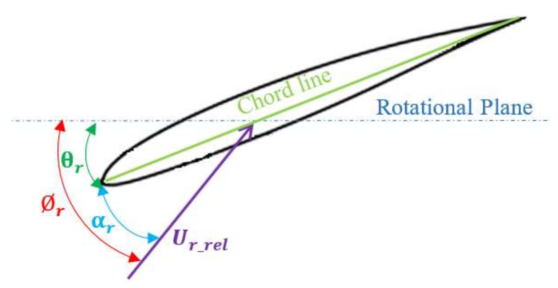
The sectional pitch angle (θr) is the angle formed between the sectional chord of the blade and the rotational plane. Pitch angle is another approach to alter generated power in pitch-regulated turbines. Pitch angle is also utilized in adjusting twists along the span of optimized blades.
The sectional angle between the local relative flow velocity (Ur_rel) and the sectional chord (cr) of the blade is termed the local angle of attack (Uαr) and is given as
where the subscript r denotes the radial location and Ør is the angle between Ur_rel and the rotational plane. This local angle, Ør, is calculated as follows.
where α and α′ are, respectively, the axial and tangential induction factors. Figure 1 is a schematic demonstration of all the sectional angles discussed above.
The blockage in turbines occurs when turbines operate in confined flows. Blockage increases the flow speed through the turbine and alters its efficiency [7,20]. The blockage intensity is designated by the blockage ratio () which is calculated as follows
where is turbine’s swept area and is the cross-sectional area of the flow domain the turbine operates in.
3. Computational Fluid Dynamics
The turbine operating under various configurations was numerically analyzed using the Reynolds-averaged Navier–Stokes (RANS) turbulence model in conjunction with the moving reference frame technique to conduct the parametric assessment of blockage effects on turbine performance. The simulated turbine geometry, mesh, and used turbulence model are discussed in this section.
3.1. Geometry and Meshing
The rotor used had three blades. The selected hydrofoils for the blades were Eppler 395. The Eppler 395 hydrofoil was chosen due to its high lift (Cl) to drag (Cd) ratio [32]. The blades were untwisted and untapered. The untwisted, untapered blades were used to reduce the number of factors altering the turbine performance and consider only those that may affect the blockage behavior. The rotor radius was 15.557 cm (6.125 in.), blade length was 13.970 cm (5.5 in.), and the hub radius was 1.587 cm (0.625 in.). This work considered different chord lengths to study σ effects on the blockage behavior and eliminate the effects introduced if the solidity was varied by altering the number of blades.
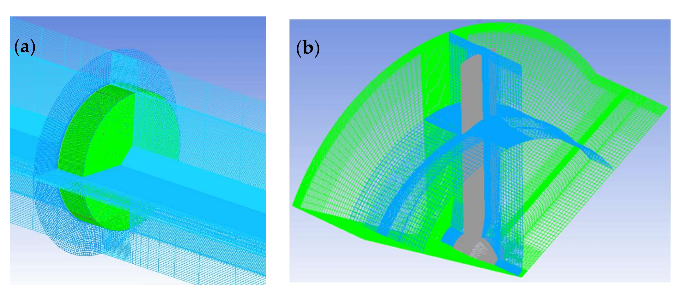
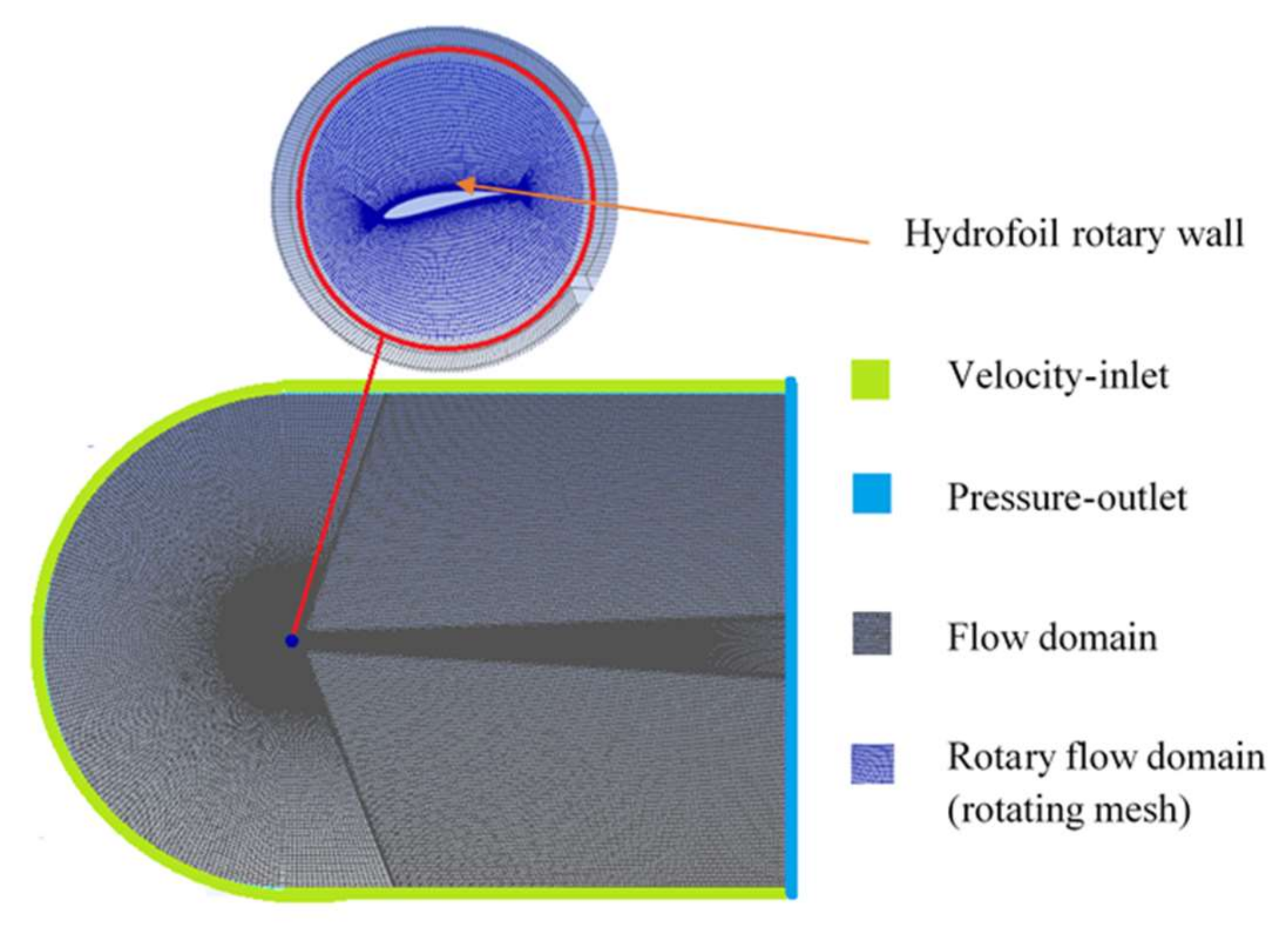
The computational domain had an inner rotor domain and an outer flow domain. The outer flow domain cross-sectional dimensions were varied to alter for the parametric study of the blockage effects. Within the outer flow domain, a cylindrical block corresponding to the inner rotor domain (colored green in Figure 2a) was removed to provide room for the inner rotor domain to be added later. This cylindrical block and the outer flow domain were concentric for all cases except for the validation case where this block was positioned at the same depth as the actual tested turbine. The outer flow domain has a streamwise length of approximately 35 rotor diameters (35 Dia.). The distance between the flow domain entrance and the rotor domain cylindrical block was a 10 Dia. Length.
Only one-third of the rotor was constructed each time utilizing both MATLAB and ANSYS 19.1/ICEM. MATLAB was used to ease altering the geometrical data of blade pitch angle and chord length. The blocking technique in ICEM can provide an easy way of building structured hexahedral meshes. Therefore, it was employed to construct the inner rotor domains and the outer flow domain volumes. The grids were assigned to the edges of the blocks of the two domains, with denser grids set near the rotor surfaces. Finally, the hexahedral mesh was generated and inspected for its quality. Figure 2a,b show a meshed outer flow domain and meshed one-third inner rotor domain, respectively.
All the meshed domains (the three domains of the inner rotor and the domain of the outer flow) were combined in ANSYS 19.1/Fluent for solving. Because the entire computational domain comprised both stationary (Ω = 0) and moving fluid regions, non-conformal interfaces were created to divide them. The non-conformal interface allowed for an efficient linking between neighboring blocks by transferring flow properties between non-matched nodes when the moving reference frame (MRF) approach was implemented. The flow properties could be determined because the interfaces allowed for the passing of the velocity and velocity gradient. Table 1 below lists all specifications of the hydrodynamic and design parameters that were considered in this work.
3.2. Turbulence Modeling
3.2.1. SST k-ω Model
The SST k-ω turbulence model, developed by Menter [33], was used to solve the RANS equations for evaluating the turbine’s performance. The SST k-ω model can manage the adverse pressure gradient and stalled flow; therefore, it is widely used for simulating wind and water turbines [14,34,35,36,37]. This enables the model to reliably estimate the stalling characteristics that dominate the suction side of the blades when the rotor is operating at optimum conditions [35]. The degree of eddy viscosity in the wake determines the ability of turbulence models that employ the eddy viscosity technique to anticipate the flow separation generated by a strong adverse pressure gradient [33]. Controlling the eddy viscosity within the wake region of the boundary layer (BL) in unfavorable pressure gradient regions requires preserving the proportionality between the principal turbulent shear stress and turbulent kinetic energy. [33,38]. To overcome the shortage of two-equation models calculating the separation caused by the adverse pressure gradient, the eddy viscosity formulation in the SST k-ω model was adjusted to account for the principal turbulent shear stress transport effects. The shear-stress transport k-ω model incorporates the k-ω model at wall vicinity BL and switches to a modified k-ε model at far-field regions [14,33]. The SST k-ω model governing equations are given by
where is blending function used to switch between the two models, is the dynamic viscosity, is the turbulent eddy viscosity, is the turbulence kinetic energy, is the specific dissipation rate, and , , , and are the model’s constants. is Reynolds-stress tensor and is calculated as
where is the mean strain-rate tensor. The definitions of the other variables and constants presented in the model’s equations can be found in the original work [33].
3.2.2. Moving Reference Frame
The flow around any rotary machine becomes unsteady when observed from a stationary reference frame. Additionally, centrifugal forces in the rotating turbines accelerate the radial flow along the blade’s span. Similarly, the Coriolis forces accelerate the flow along the blade’s chord. This change in the flow behavior affects the stall mechanism [39,40]. The numerical modeling of HAHkTs becomes challenging when these rotating effects are combined with the turbulent flow, and solving the turbulent model’s governing equations in a stationary frame of motion necessitates a great computational effort [14,41]. To mitigate these rotational effects, the turbulence model incorporated the MRF approach, so flow around the operating rotor is steady with respect to this moving frame. The MRF equation (Equation (14)) is formulated to have additional terms that account for the rotational forces [42].
When a turbine operates at a constant rotational speed, Ω, and with a zero yawing angle with respect to a steady incoming stream, then MRF equations using relative velocity formulation are as follows [14,43,44]
where Urel is the relative velocity defined as . The centrifugal forces and Coriolis forces in Equation (14) are accounted for by and terms, respectively. The term represents the pressure gradient, and the term describes the viscous stress tensor, which is calculated as
where is the identity tensor.
3.2.3. Model Setup
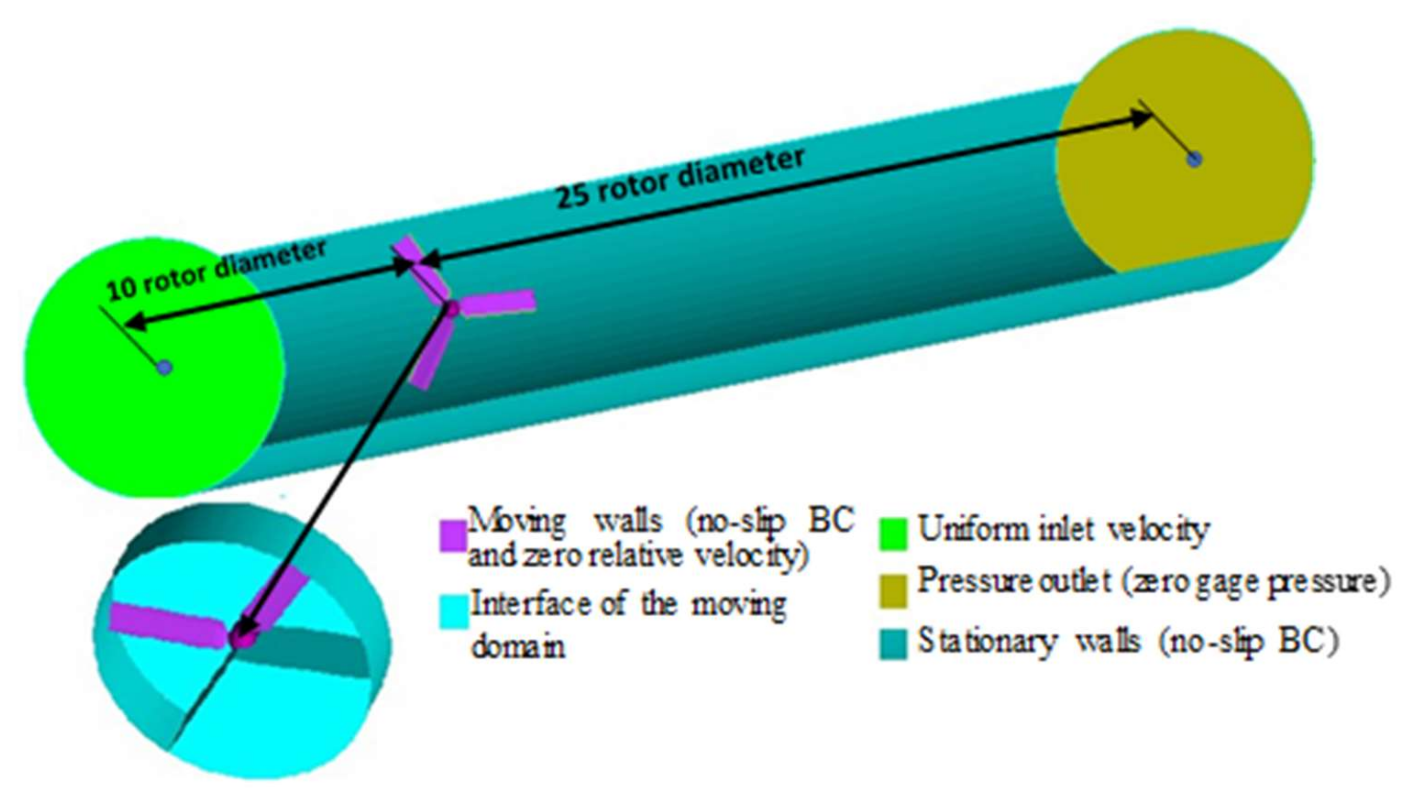
The CFD simulation was performed using ANSYS 19.1/Fluent commercial software. The flow was considered steady and incompressible. Figure 3 illustrates the boundary conditions of a hydrokinetic turbine operating in an outer cylindrical confined flow. Part of the outer flow walls and some of the interfaces around the rotor were hidden to provide a better illustration.
The water tunnel inlet was positioned about 10 rotor diameter (dia.) upstream the rotor and was given a uniform velocity of 1.5 m/s. This velocity was within the practical range of typical sites for the deployment of hydrokinetic turbines [45]. The inlet’s turbulent intensity () was set to 1%. The inlet’s turbulence length scale () was set such that , where is the chord length. The outlet was located 25 dia. downstream of the rotor. The outlet turbulence length scale () was given a value similar to. For the implementation of the MRF method, the inner flow domains neighboring the blades were adjusted to a rotational frame of motion and given a rotational speed similar to the rotating rotor. Other BCs are defined in Figure 3.
The flow governing equations were solved using second-order upwinding discretization schemes. The resolving for velocity and pressure was achieved in a coupled manner using the coupled scheme. The convergence for all solution variables was reached when residuals were less than and when the moment, thrust, and mass flow were settled.
3.3. Grid Independent Investigation
The effects of mesh size on the final solution were investigated. The goal was to locate the optimum mesh resolution that yields less change in the solution while reducing the computational effort studied. The size of the mesh of the rotor with the largest chord length, c = 6.35 cm (2.5 in.), and a pitch angle of = 10° was altered, and its moment coefficient (CM) was documented. The rotor was operated at a flow speed of 1.5 m/s and a rotational speed of 376 RPM. The residuals were decreased below if the moment and thrust did not converge. The initial wall spacing of the blade surfaces () was maintained at to resolve the boundary layer (BL). The optimum rotor mesh size was approved at around 4.06 million elements (The total model element number, including outer domain, was about 6.171 million). At this mesh size, the resulting change in CM was about 0.019% when the rotor domain grid was uniformly increased from 4.06 million to 7.322 million elements. Increasing the mesh size larger than 4.06 million elements did not yield a noticeable change in CM. For this optimum mesh size, the number of grids along the hydrofoil was 110.
3.4. Experimental Validation
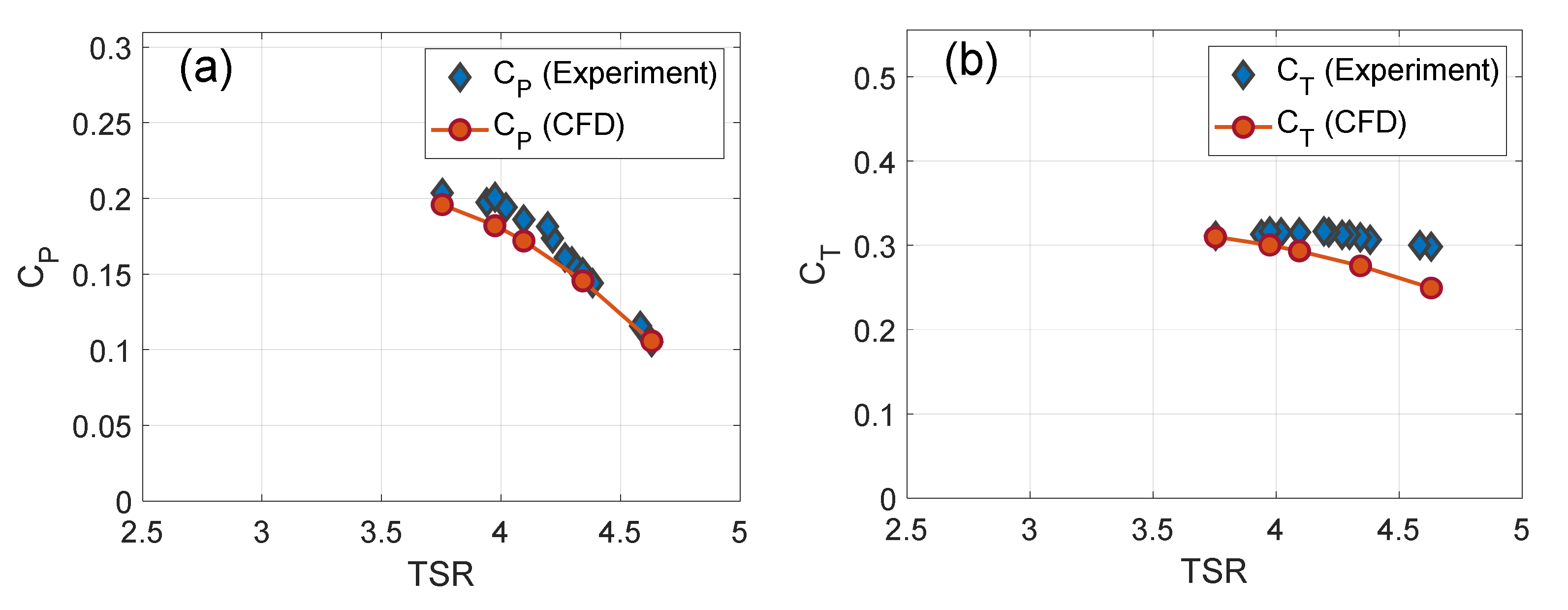
Three blades with a chord length of 1.676 cm (0.66 in.) were manufactured of composite; then, the rotor was assembled and operated in the water tunnel to validate the power and thrust coefficients predicted using CFD with the k-ω SST turbulence model. The details of the experimental setup for measuring power and thrust coefficients are discussed in [16]. The pitch angle was set to 20°, and the flow speed was set to 0.91135 m/s. This pitch angle of 20° was selected to decrease the blades bending under the flow forces. The rotor radius was 15.557 cm (6.125 in.), and the blockage resulting from placing this rotor in the water tunnel was around 41.35%.
In Figure 4a, due to the stall delay, the CP versus TSR curve did not experience a decline in its magnitude as TSR decreased. The stall delay caused a longer span of the blade to operate at angles of attack below the stall angle [46]. Consequently, as the applied load on the turbine increased and reached a value more significant than the turbine’s generated torque, the rotor came to a halt. The validation results in Figure 4a show that the CP satisfactorily agreed with the water tunnel measurements. The CT was slightly underestimated and then likely overestimated as TSR decreased from 4.54 to values less than 3.75 (Figure 4b). The close match of the steady RANS results to the experimental measurements provided confidence in the steady approach. Therefore, it was used in the study of the blockage effects on the turbine performance.
4. Evaluating the Operational Rotational Speed
Before the start of running the 3D CFD cases for the blockage effect investigation, it is essential to define the range of the operational rotational speed (Ω) or tip speed ratio (TSR) within which the selected rotors with different solidities (different chord lengths) operate. These ranges of Ω or TSR for the selected rotors were evaluated using a modified blade element momentum (BEM) model [47]. The BEM theory is a very common tool used in predicting the performance of unconfined HAWTs due to its relative simplicity and minimal computational efforts compared to the higher fidelity CFD methods. BEM theory can only be used to evaluate the turbine performance in open flows; therefore, it was not considered any further in the blockage effects study. Several textbooks and papers report a detailed discussion of the BEM theory derivation and employed corrections [1,48,49,50,51,52].
The hydrodynamic characteristics (Cl and Cd) for all used chord lengths required by the BEM model were obtained from 2D CFD models utilizing the SST k-ω turbulence model. The angle of attack, α (α = θ in 2D flow), was altered by rotating the meshes of the hydrofoil and the surrounded flow domain from −10° to 30° with an increment step of 1°. The boundary conditions for this 2D CFD model are illustrated in Figure 5. The flow speed at the inlet was set at 1.5 m/s, which was the same flow speed considered in the blockage investigation. To account for the rotational and 3D effects, the Cl and Cd were modified using models from [53] and [54], respectively. These rotational and 3D effects were made based on a hydrofoil located at 80% of the considered blades spans as this was the recommended design span [41]. The modified Cl and Cd were then extrapolated over a broad range of α (±180°) using the Viterna model [55]. This broad range of α is needed by the BEM model while searching for the solution parameters iteratively.
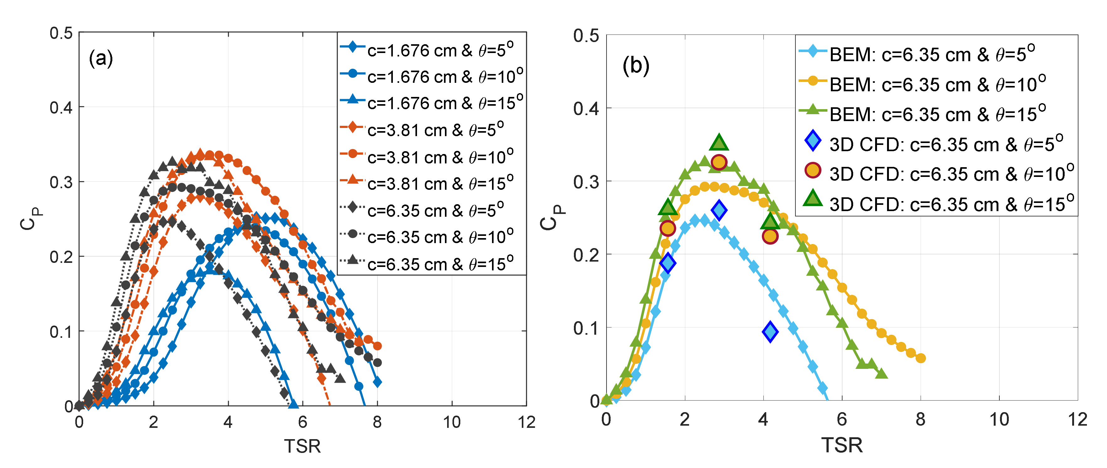
The BEM prediction of CP for the different considered rotors is shown in Figure 6a. The BEM prediction of a rotor with a blade chord length of 6.35 cm (2.5 in.) was verified against 3D CFD unconfined model ( 4.168%), and the results are shown in Figure 6b. The blockage ratio of is considered effectively unblocked [21]. The BEM slightly underestimated the CP peak and then started to overestimate CP as TSR increased. This was likely attributed to the used 3D effects correction models, which were considered at one representative radial location and using one representative rotational speed (Ω = 200 RPM). Additionally, the 3D correction model is designed for larger blades where the aspect ratio (r/c) is less than one over most of the blade span.
5. Experimental Design
The effects of several hydrodynamic and geometric parameters and their interactions on the blockage behavior and, consequently, on the turbine performance were quantitatively evaluated using a validated 3D CFD model and design of experiments (DOE) approach. The change in CP and CT (i.e., and ) as a result of the blockage effects were the response variables of the DOE and are defined in Equation (16).
where x stands for either power or thrust, ∆Cx is the response variable, and are the coefficients when a turbine operates in confined and unconfined flows, respectively. The independent parameters (factors) considered in the DOE study are blockage ratio (), solidity (varied by changing chord length), tip speed ratio (TSR), and the pitch angle (). These parameters affect the CP and CT and are likely to affect the blockage behavior. A full factorial DOE investigation was considered with four parameters and three levels per each. This required 81 3D CFD runs (). The considered parameters and their levels are listed in Table 2.
The same levels of , θ, and TSR are considered for the unconfined rotor case with = 4.168% ( is considered effectively unblocked [21]). This increased the number of 3D CFD runs to 108. Additionally, the total number of meshed models for all cases was 36. These unconfined cases served as a baseline to calculate the response variables (∆CP and ∆CT) due to blockage effects.
6. Results and Discussion
6.1. Influence of the DOE Parameters on the Blockage Behavior
The influences of the blockage ratio, solidity, pitch angle, and tip speed ratio on how the blockage affects the turbine performance are studied in this section. Based on the BEM results in Figure 6, the operational TSR (TSR at the CP peak) for the rotors with c = 6.35 cm ( = 0.191) and c = 3.81 ( = 0.115) was insensitive to the alteration of θ. Thus, for these rotors, when comparing performances within the selected range of TSR, the possibility of the change in performance due to the shifting of the CP vs. TSR curve is eliminated. For this reason, this work started the analyses of the DOE parameters using the rotor with the highest solidity ( = 0.191).
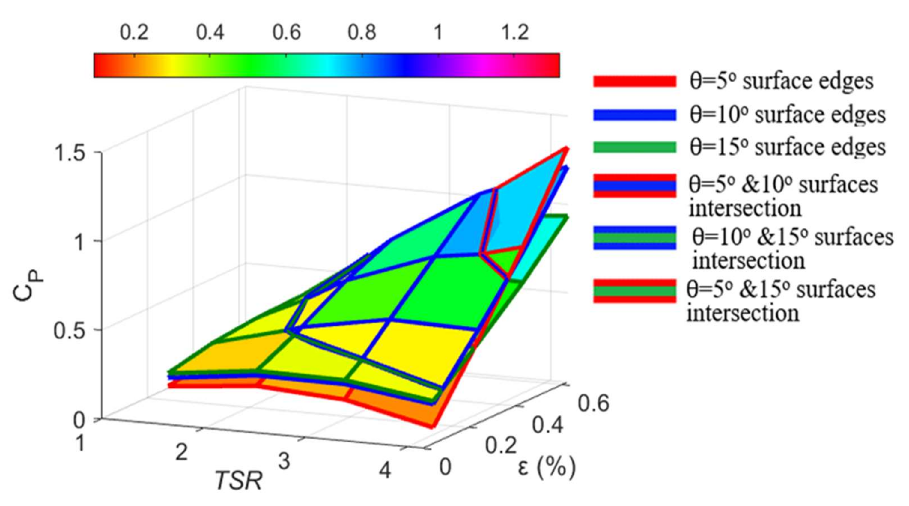
Response surfaces that represent the change in performance, CP, of the highest solidity rotor with varying tip speed ratio, TSR, and blockage ratio, are represented in Figure 7. Each response surface was generated at a fixed pitch angle, θ. Different edge colors were used to differentiate between the surfaces. The intersections between surfaces were indicated by parallel curves that were given the same colors as the edges of the intersecting surfaces. This was also illustrated in the legend of Figure 7. This figure shows that the blockage effects on the turbine performance increase with increasing TSR for all pitch angles. Figure 7 also shows that the surface that represents θ = 5° was the most affected by the blockage as indicated by the surface with the red edges. This surface changed from the lowest CP to the highest CP as the TSR and increased. Additionally, the performance of this high solidity rotor when θ = 5° and 10° was larger than unity (i.e., CP > 1) at the extreme level of confinement and highest rotational speed. This was caused by the large increase in the kinetic flux passed through and around the highly confined rotor. Meanwhile, the power coefficient was calculated via normalizing the extracted power from the augmented confined kinetic flux by the kinetic flux at the upstream undistorted region (i.e., unconfined environment).
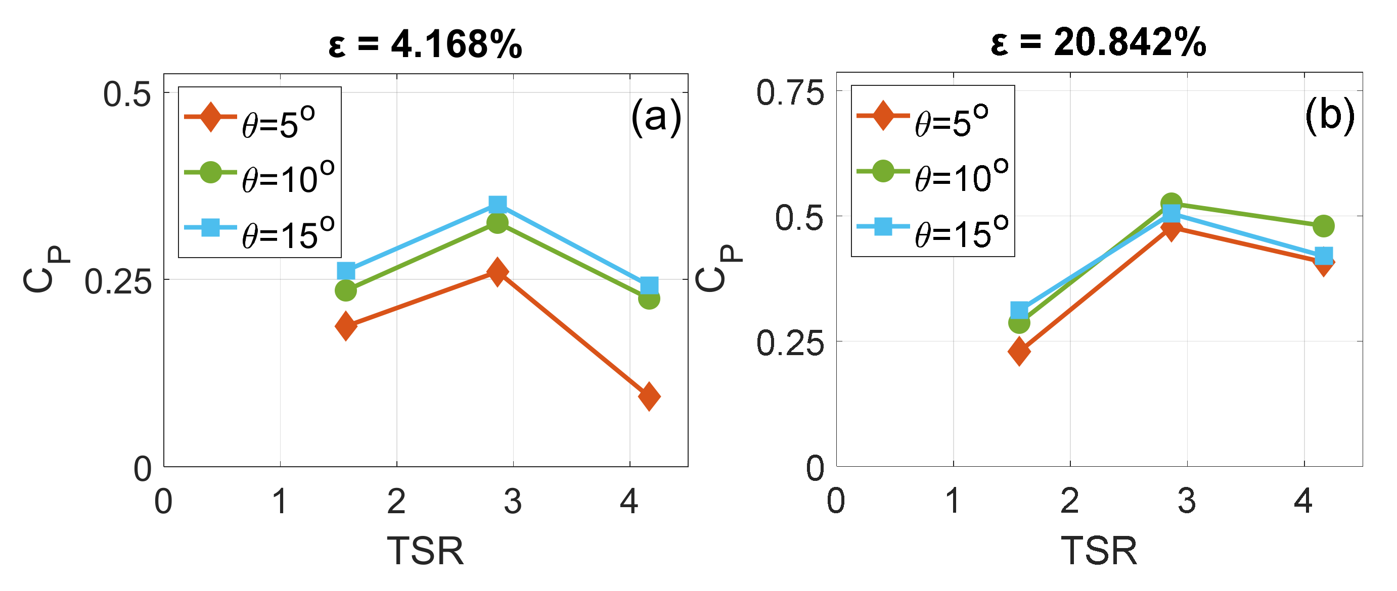
For simplified illustration, the change in CP with TSR and θ is presented for each blockage ratio separately in Figure 8. The increase and then decrease in CP as TSR increase in Figure 8a,b indicates that the CP peak was located within this range of TSR. On the other hand, this pattern of increase and decrease in the CP curve is not observed or less pronounced in Figure 8c,d, which indicates that the CP peak was not within this range of TSR at these relatively high levels of . The increase in the blockage caused a slight shift in the CP peak to higher TSRs. This was attributed to the fact that increasing the blockage (i.e., decreasing the tunnel’s cross-sectional area) augmented the flow around the rotor. Because the TSR range was fixed, the angle of attack increased (see Equations (7) and (8)), and thus larger portions of the blades’ spans were stalled. The rotors need to rotate faster to bring the angles of attack along the blades at or below the stall angle. This means the rotors need to operate at higher TSR to reach the CP peak. Additionally, in Figure 8a–d, it is clear that at the highest TSR, the smaller the θ, the faster the CP increased with increasing the ε.
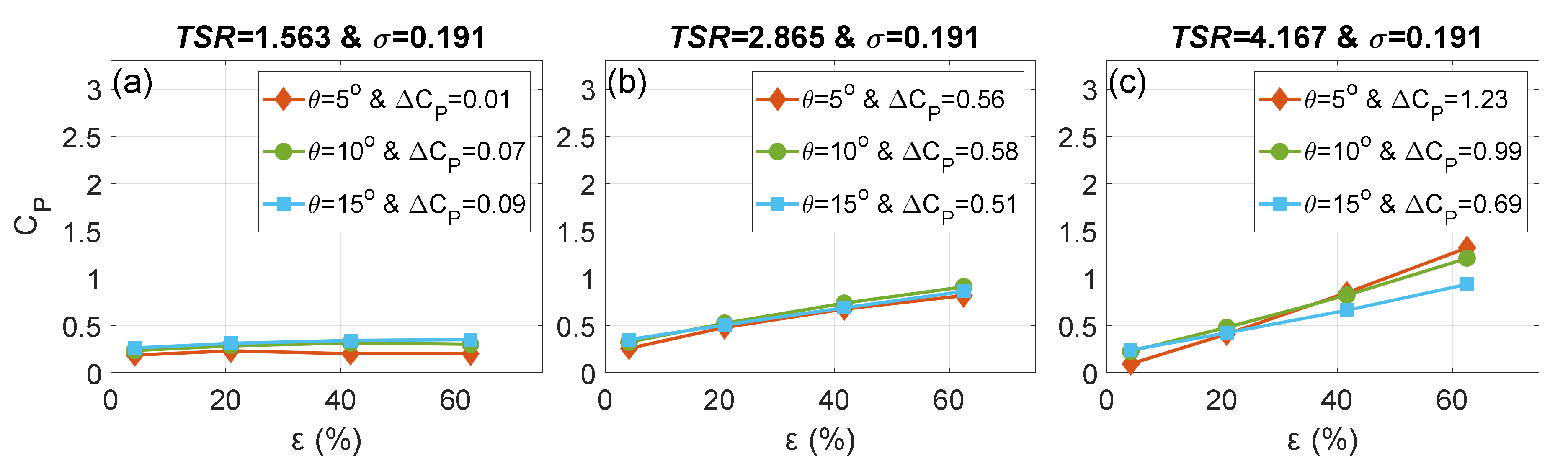
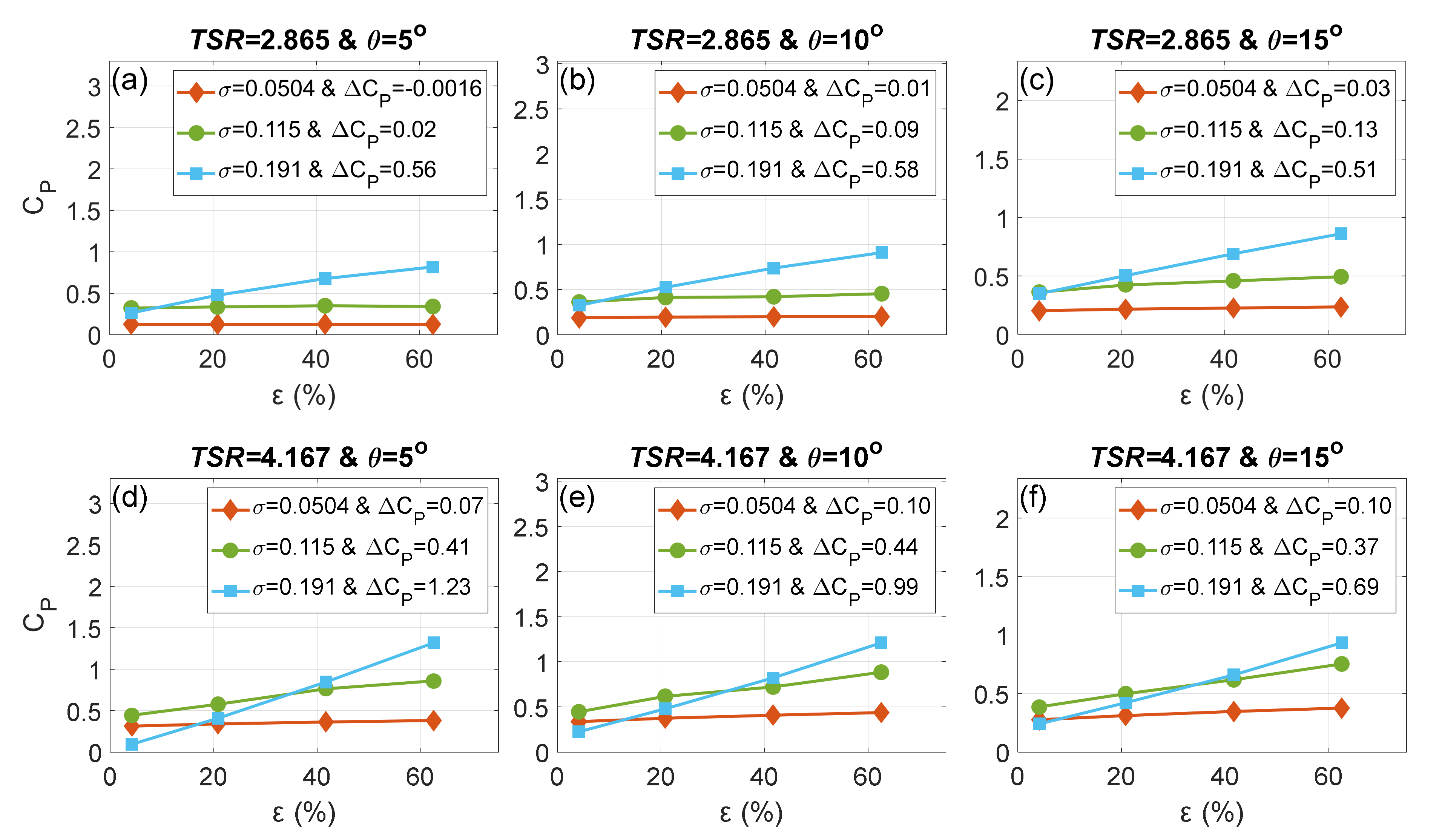
To further understand how varying θ influences the blockage effects on CP, the relationship between CP vs. ε was plotted for all pitch angles at fixed TSRs. The results are shown in Figure 9. The ∆CP in the legend represents the change in performance due to changing the blockage from ε = 4.168 % to ε = 62.533%. The similar curves slope in Figure 9a,b indicates that varying θ has insignificant effects on how the blockage alters the turbine performance at this relatively low range of TSRs. When TSR = 1.563, the change in ∆CP as a result of varying θ was 0.08 (e.g., ) as seen in Figure 9a. The change in ∆CP caused by changing θ was 0.07 when TSR = 2.865 (Figure 9b).
Referring to Figure 6b, which shows the performance of the unconfined high solidity rotor, The TSR of 1.563 is located at the stalled region. At this stalled region, any increase in flow speed as a result of increasing the blockage will make the flow separation at the suction side of the blade worse. In Figure 9a, the increase in θ at this TSR was not large enough to bring the range of angles of attack along the extremely stall-dominated blade to values close to or below the optimum angle of attack (stall angle). Therefore, the performance was unresponsive to θ variation as the blockage increased.
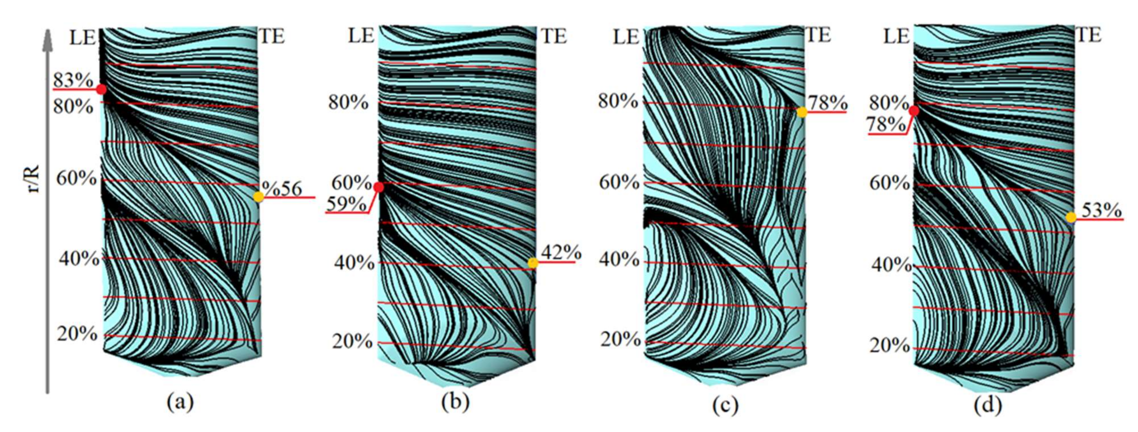
The TSR = 2.865 was located slightly at the right of the CP peak (Figure 6b). The separation also existed at this TSR but with less intensity and covered a relatively smaller portion of the blade span for this unconfined rotor [46]. To examine the effects of the blockage ratio and angle of attack on flow separation and thus analyze the results in Figure 9b, Figure 10 was generated. Figure 10 utilizes surface streamlines to detect the flow behavior. The fully attached flow at the blade outboard is denoted by a red dot at the leading edge (LE) and an orange dot at the trailing edge (TE). Only Figure 10c does not have the red dot because the flow is not fully attached to all LE span. The percentage numbers represent the ratio of the radial distance to the rotor diameter (r/R). Increasing the pitch angle resulted in expanding the area of the fully attached flow, as observed when comparing Figure 10a to Figure 10b or Figure 10c to Figure 10d. However, the CP was still insensitive to θ alteration (Figure 9b), which is similar to the previous lower TSR. This was likely due to the insignificant effect of the change in lift and drag coefficients at the regions of fully and partially attached flows. However, ∆CP at this TSR was more significant than in the previous case (TSR = 1.563). The increase in blockage augmented both the flow and the angle of attack (see Equations (7) and (8)). Therefore, as ε increased, the fully attached flow covered a smaller outboard region of the blade; this can be observed when comparing Figure 10a to Figure 10c or Figure 10b to Figure 10d. However, the rise in the lift due to the increase in blockage and thus flow speed (e.g., increase in Reynolds number) outperformed the decrease in the lift due to the increase in flow separation. Therefore, the ∆CP when TSR = 2.865 (Figure 9b) improved compared to that when TSR = 1.563. The increase in lift coefficients along the blade due to the increase in blockage when TSR = 2.865 and θ = 10° was verified by monitoring the change in moment coefficient (). The increased from 0.111 to 0.31 as ε increased from 4.168% to 62.533%.
The improvement in ∆CP was more pronounced when TSR was 4.167, as indicated by the slopes of the lines and the legend in Figure 9c. This TSR is located at the right side of the CP peak (see Figure 6b), where the fully attached flow covered a larger portion of the blade than the previous TSRs. Therefore, the increase in blockage augmented the angles of attack along the blade to levels close to the optimum value, and thus the ∆CP was larger compared to the lower TSRs. It was also observed that varying the pitch angle affects the blockage behavior at this TSR of 4.167. The pitch angle of 15° had the lowest ∆CP as blockage increased. That was because θ = 15° caused the angles of attack along most of the blade span to decrease to values below the optimum angle of attack, which lowered the lift and, thus, the moment.
The other blades with smaller chords showed similar behaviors as in Figure 9a–c but with smaller ∆CP as solidity decreased.
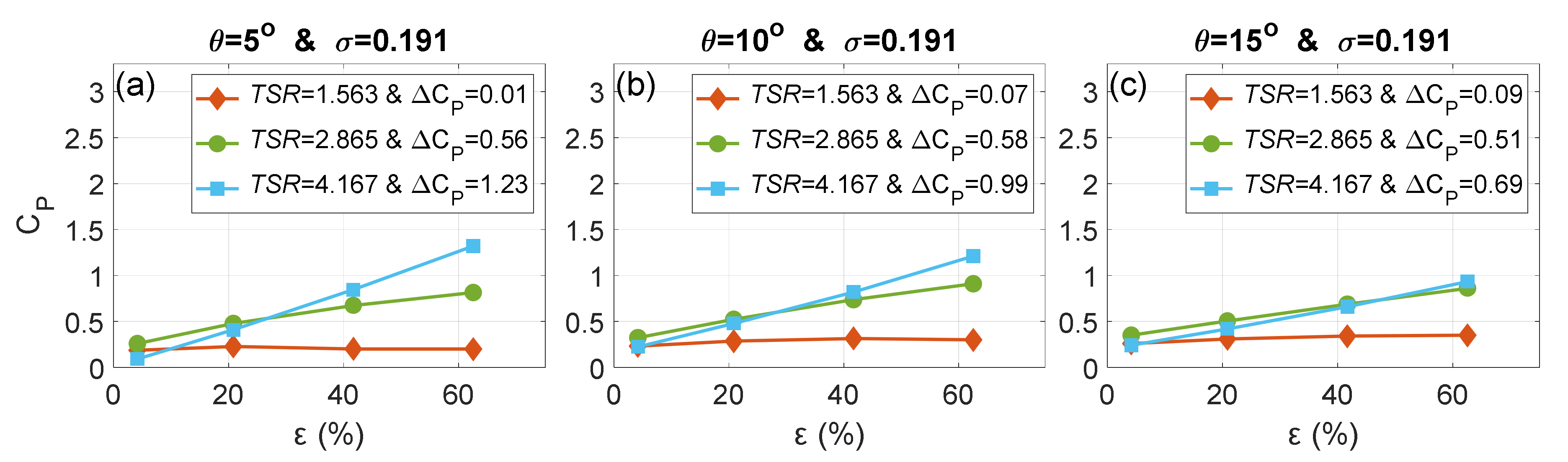
The individual effect of TSR on blockage behavior was also investigated, and results are shown in Figure 11. For all considered pitch angles, the rate of increment of CP with respect to ε increased with increasing the TSR (i.e., ∆CP is proportional to TSR). The proportionality between blockage effects and TSR (i.e., rotational speed) was partly attributed to the augmented wake turbulence and elevated bypass flow [5]. The blockage that influences the performance of a confined turbine comprises both the rotor blockage and wake blockage [56], where the latter is mainly affected by rotor rotational speed. The increase in rotational speed results in a stronger wake boundary and stronger wake blockage [5], which further enhances the kinetic flux and thus the turbine performance.
The lowest TSR of 1.563 showed minor CP enhancement (i.e., ∆CP was very small) as the blockage increased. As the flow speed increased with increasing the blockage and as the turbine started to decrease its rotational speed under loading, the stall started at the inboard region of the untwisted blades and then propagated towards the tip under Coriolis and centrifugal force effects [40,57]. The large stall-dominated portion of the blade span at this low TSR caused a drop in the lift, which unfavorably affected the turbine performance. As rotational speed increased, the range of angles of attack along the blade span was lowered, where angles of attack were smaller towards the tip. That means as TSR increased, the separation became less intense and covered a smaller portion of the blade, mostly at the inboard segment. Thus, at the elevated TSRs, as the flow speed increased due to increased blockage, an increasing portion of the outboard of the blade had angles of attack that increased to levels below or near the optimum angle, which enhanced the performance (i.e., ∆CP increased).
It was also observed that as pitch angle increased, the deviation between the TSR lines representing the CP vs. decreased. Because a larger portion of the blade span was stalled at TSR = 2.865, the line slope was affected less by increasing the θ compared to TSR = 4.167 (this was explained in Figure 9 discussion). The slope of the TSR = 4.167 line was decreased the most and approached the slope of the TSR = 2.865 line as the pitch angle increased to 15°. This was again due to the decrease in the angles of attacks below the optimum value.
The other blades showed similar behaviors; the larger TSR, the higher the performance, though the slopes of TSRs lines tended to decrease with decreasing the solidity. Additionally, the plots are not included as solidity effects are discussed in the following figure.
The effect of solidity on turbine performance operated at different levels of confinement was also investigated and presented in Figure 12. Because the blockage has insignificant effects at a TSR of 1.563, this low TSR was not included in Figure 12. It was observed that the blockage effects increased with increasing solidity. The ∆CP was proportional to σ, and this proportionality increased with increasing TSR. For TSR of 2.865 (Figure 12a–c), the highest solidity rotor (σ = 0.191) showed the highest values of ∆CP for all pitch angles while the lower solidities (σ = 0.0504 and 0.115) showed minimal values of ∆CP at all pitch angles. The ∆CP with a negative sign in Figure 12a indicates a slight decrease in performance due to increasing the blockage for this lowest solidity rotor with a pitch angle of 5°. This was due to the increase in stall effects as a result of increasing the U/ωr ratio.
The increase of blockage effects with increasing solidity was more pronounced at a TSR of 4.167 (Figure 12d–f). Additionally, the performance of the highest solidity rotor (σ = 0.191) changed from the poorest to the highest as increased from 4.168% to 62.533% for all tested pitch angles. A rotor with higher solidity (larger chord length) has a larger lift surface yet experiences a higher flow impedance through its swept area. Therefore, the kinetic energy passing the unconfined highest solidity rotor was the lowest, which was reflected in the poor performance. As the flow increased due to the increase in the blockage, the passing kinetic flux increased, and the performance of the highest solidity rotor with the largest lift surface improved the most for all tried pitch angles (Figure 12d–f).
6.2. Analysis of Variance of the DOE Parameters
The effects of the hydrodynamic and geometric parameters on the blockage behavior were quantitatively evaluated using analysis of variance (ANOVA). The null hypothesis considered in this study assumes that the change in factors’ levels (i.e., levels of ε, θ, and TSR) does not have a significant effect on the response variables (i.e., ∆CP and ∆CT). If ANOVA output, p-value, is less than a predetermined significance level (0.05 used in the current study), the null hypothesis is rejected, concluding that: a change in at least one of the treatment combinations (i.e., a set of factors’ levels) results in a statistically significant change in ∆CP or ∆CT. This helps to identify which of the selected factors and factors’ interactions affect the blockage behavior.
The p-value of the model in Table 3 is smaller than 0.05, indicating that the model is significant, and the null hypothesis can be rejected. Moreover, the statistical significance of the effect of the four factors and their interactions on ∆CP were tested, and results are also listed in Table 3. The p-values for all linear terms are less than 0.05, indicating that their effects on ∆CP are statistically significant. For the 2-way interactions, only the p-value from the interaction between blockage and pitch angle (ε*θ) is greater than 0.05; therefore, this interaction does not significantly affect the response variable, ∆CP. All other 2-way interactions have p-values less than 0.05; therefore, their effects on ∆CP are statistically significant. For the 3-way interactions, both *ε*θ and ε*θ*TSR interactions do not have a significant effect on the response variable, ∆CP, while *ε*TSR and *θ*TSR interactions do.
Analysis of variance for the effects of the design parameters on the other response variable (∆CT) was conducted and presented in Table 4. The p-values for all model, linear, and 2-way interactions terms are less than 0.05, indicating their statistically significant effects on ∆CT. The 3-way interactions terms also have p-values less than 0.05, and their effects are statistically significant, except the term ε*θ*TSR, which has p-values of 0.143.
The 4-way interactions were not included initially to prevent the model from being saturated (i.e., not enough degrees of freedom for error). However, when a 3-way interaction term was excluded, the 4-way interactions showed p-values greater than 0.05 for both ∆CP and ∆CT. This means the 4-way interactions do not have significant effects on the response variable.
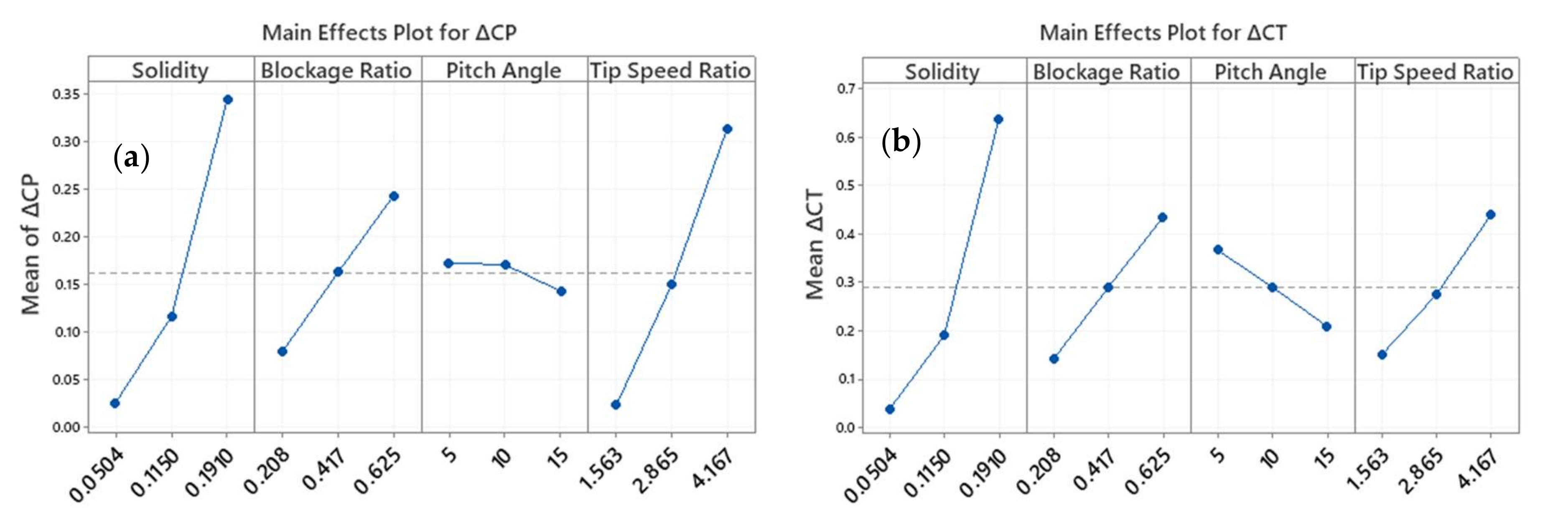
Figure 13 shows the main effects plots to inspect differences between levels and means for every factor. If various levels of a given factor influence a response variable differently, then the main effect for that factor exists. In other words, if a line in Figure 13 is tilted, then the main effect exists. The steeper the line, the larger the main effect is. From Figure 13, solidity, blockage ratio, and tip speed ratio have proportional relationships with ∆CP and ∆CT. However, the pitch angle is inversely proportional to ∆CP and ∆CT. The order of the main effect intensity of the factors on both response variables is such that solidity has the highest effect, followed by blockage ratio, tip speed ratio, and then pitch angle, which has the least effect on ∆CP and ∆CT.
7. Practical Implications
Practical implications for a turbine operating in confined flow are as the following:
- When designing a confined hydrokinetic turbine, designers should be aware of the sensitivity of the design variables to the confinement effects.
- After optimizing the turbine for an open environment, further considerations should be given toward design parameters. Priority should be given in the following order: the solidity, blockage ratio, rotational speed, and pitch angle.
- Interaction effects should also be considered; for example, the performance of the highest solidity rotor changed from the lowest in an open flow (due to the increased flow impedance) to the highest in a confined flow (due to the increased kinetic flux).
8. Conclusions
CFD models were developed to provide a broad insight into the blockage effects on the turbine’s performance. The following is a summary of the most important findings:
- CP was insensitive to θ alteration at relatively low TSRs as ε increased. The effect of varying θ was noticeable at the high TSR. The ∆CP was inversely proportional to θ at the TSR of 4.167. That was due to the decrease in the angle of attack to levels below the optimum values.
- For all pitch angles, the rate of increment of CP with respect to ε was proportional to the TSR. This proportionality was attributed to the augmented wake turbulence and the improvement in the angles of attack along the blade span due to the increase in rotational speed.
- The blockage effects were proportional to the solidity level, and this proportionality increased with increasing TSR. Additionally, the performance of the highest solidity rotor changed from the poorest to the highest as increased.
The effects of ε, θ, and TSR on the blockage behavior were quantitatively evaluated using the analysis of variance, ANOVA. The ANOVA examined the effects of varying the DOE parameters on the turbine performance and showed the following:
- The ε*θ,*ε*θ, and ε*θ*TSR interactions do not have significant effects on ∆CP. All other linear, 2-way, and 3-way interactions are statistically significant in affecting the ∆CP.
- All model, linear, 2-way, and 3-way (excluding ε*θ*TSR) interactions are statistically significant in affecting the ∆CT.
- All 4-way interactions do not have significant effects on both response variable
The order of the intensity of the main effect of the factors on both response variables was also analyzed. The solidity was found to have the highest effect on both ∆CP and ∆CT, followed by blockage ratio, tip speed ratio, and then pitch angle.
Author Contributions
Conceptualization, A.A. and V.G.M.; methodology, A.A and V.G.M.; software, A.A.; validation, A.A.; formal analysis, A.A.; investigation, A.A.; resources, V.G.M.; data curation, A.A.; writing—original draft preparation, A.A.; writing—review and editing, V.G.M.; visualization, A.A.; supervision, V.G.M.; project administration, V.G.M.; funding acquisition, V.G.M. All authors have read and agreed to the published version of the manuscript.
Funding
This research was funded by University of Minnesota Grant-in-Aid of Research, Artistry and Scholarship, grant number 468572.
Institutional Review Board Statement
Not Applicable.
Informed Consent Statement
Not Applicable.
Data Availability Statement
Not Applicable.
Conflicts of Interest
The authors declare no conflict of interest.
References
- Burton, T.; Jenkins, N.; Sharpe, D.; Bossanyi, E. Wind Energy Handbook; John Wiley & Sons: Hoboken, NJ, USA, 2011. [Google Scholar]
- Batten, W.M.J.; Bahaj, A.S.; Molland, A.F.; Chaplin, J.R. Hydrodynamics of marine current turbines. Renew. Energy 2006, 31, 249–256. [Google Scholar] [CrossRef] [Green Version]
- Aghsaee, P.; Markfort, C.D. Effects of flow depth variations on the wake recovery behind a horizontal-axis hydrokinetic in-stream turbine. Renew. Energy 2018, 125, 620–629. [Google Scholar] [CrossRef]
- Bahaj, A.; Myers, L.; Rawlinson-Smith, R.; Thomson, M. The effect of boundary proximity upon the wake structure of horizontal axis marine current turbines. J. Offshore Mech. Arct. Eng. 2012, 134, 021104. [Google Scholar] [CrossRef]
- Kolekar, N.; Banerjee, A. Performance characterization and placement of a marine hydrokinetic turbine in a tidal channel under boundary proximity and blockage effects. Appl. Energy 2015, 148, 121–133. [Google Scholar] [CrossRef]
- Ryi, J.; Rhee, W.; Hwang, U.C.; Choi, J.-S. Blockage effect correction for a scaled wind turbine rotor by using wind tunnel test data. Renew. Energy 2015, 79, 227–235. [Google Scholar] [CrossRef]
- Kinsey, T.; Dumas, G. Impact of channel blockage on the performance of axial and cross-flow hydrokinetic turbines. Renew. Energy 2017, 103, 239–254. [Google Scholar] [CrossRef]
- Bahaj, A.S.; Molland, A.F.; Chaplin, J.R.; Batten, W.M.J. Power and thrust measurements of marine current turbines under various hydrodynamic flow conditions in a cavitation tunnel and a towing tank. Renew. Energy 2007, 32, 407–426. [Google Scholar] [CrossRef]
- Watanabe, S.; Yamaoka, W.; Furukawa, A. Unsteady Lift and Drag Characteristics of Cavitating Clark Y-11.7% Hydrofoil. IOP Conf. Ser. Earth Environ. Sci. 2014, 22, 052009. [Google Scholar] [CrossRef] [Green Version]
- Sun, Z.; Li, Z.; Fan, M.; Wang, M.; Zhang, L. Prediction and multi-objective optimization of tidal current turbines considering cavitation based on GA-ANN methods. Energy Sci. Eng. 2019, 7, 1896–1912. [Google Scholar] [CrossRef] [Green Version]
- Ashrafi, Z.N.; Ghaderi, M.; Sedaghat, A. Parametric study on off-design aerodynamic performance of a horizontal axis wind turbine blade and proposed pitch control. Energy Convers. Manag. 2015, 93, 349–356. [Google Scholar] [CrossRef]
- Rector, M.C.; Visser, K.D.; Humiston, C. Solidity, blade number, and pitch angle effects on a one kilowatt HAWT. In Proceedings of the 44th AIAA Aerospace Sciences Meeting and Exhibit, Reno, NV, USA, 9–12 January 2006; pp. 1–10. [Google Scholar]
- Duquette, M.M.; Visser, K.D. Numerical Implications of Solidity and Blade Number on Rotor Performance of Horizontal-Axis Wind Turbines. J. Sol. Energy Eng. 2003, 125, 425–432. [Google Scholar] [CrossRef]
- Subhra Mukherji, S.; Kolekar, N.; Banerjee, A.; Mishra, R. Numerical investigation and evaluation of optimum hydrodynamic performance of a horizontal axis hydrokinetic turbine. J. Renew. Sustain. Energy 2011, 3, 063105. [Google Scholar] [CrossRef] [Green Version]
- Sarlak, H.; Nishino, T.; Martínez-Tossas, L.; Meneveau, C.; Sørensen, J.N. Assessment of blockage effects on the wake characteristics and power of wind turbines. Renew. Energy 2016, 93, 340–352. [Google Scholar] [CrossRef] [Green Version]
- Abutunis, A.; Fal, M.; Fashanu, O.; Chandrashekhara, K.; Duan, L. Coaxial horizontal axis hydrokinetic turbine system: Numerical modeling and performance optimization. J. Renew. Sustain. Energy 2021, 13, 024502. [Google Scholar] [CrossRef]
- Madrigal, T.H.; Mason-Jones, A.; O’Doherty, T.; O’Doherty, D.M. The effect of solidity on a tidal turbine in low speed flow. In Proceedings of the 2nd European Wave and Tidal Energy Conference (EWTEC), Cork, Ireland, 27 August–1 September 2017; pp. 1–9. [Google Scholar]
- Morris, C.; Mason-Jones, A.; O’Doherty, D.M.; O’Doherty, T. The influence of solidity on the performance characteristics of a tidal stream turbine. In Proceedings of the European Wave and Tidal Energy Conference, Nantes, France, 6–11 September 2015; pp. 1–7. [Google Scholar]
- Abutunis, A.; Taylor, G.; Fal, M.; Chandrashekhara, K. Experimental evaluation of coaxial horizontal axis hydrokinetic composite turbine system. Renew. Energy 2020, 157, 232–245. [Google Scholar] [CrossRef]
- Chen, T.; Liou, L. Blockage corrections in wind tunnel tests of small horizontal-axis wind turbines. Exp. Therm. Fluid Sci. 2011, 35, 565–569. [Google Scholar] [CrossRef]
- Whelan, J.I.; Graham, J.M.R.; Peiró, J. A free-surface and blockage correction for tidal turbines. J. Fluid Mech. 2009, 624, 281–291. [Google Scholar] [CrossRef]
- Garrett, C.; Cummins, P. The efficiency of a turbine in a tidal channel. J. Fluid Mech. 2007, 588, 243–251. [Google Scholar] [CrossRef] [Green Version]
- Houlsby, G.; Draper, S.; Oldfield, M. Application of Linear Momentum Actuator Disc Theory to Open Channel Flow; University of Oxford: Oxford, UK, 2008. [Google Scholar]
- Barnsley, M.; Wellicome, J. Final Report on the 2nd Phase of Development and Testing of a Horizontal Axis Wind Turbine Test Rig for the Investigation of Stall Regulation Aerodynamics; Carried out under ETSU Agreement E.5A/CON5103/1746; 1990. [Google Scholar]
- De Arcos, F.Z.; Tampier, G.; Vogel, C.R. Numerical analysis of blockage correction methods for tidal turbines. J. Ocean Eng. Mar. Energy 2020, 6, 183–197. [Google Scholar] [CrossRef]
- Ross, H.; Polagye, B. An experimental assessment of analytical blockage corrections for turbines. Renew. Energy 2020, 152, 1328–1341. [Google Scholar] [CrossRef] [Green Version]
- Masters, I.; Chapman, J.C.; Willis, M.R.; Orme, J.A.C. A robust blade element momentum theory model for tidal stream turbines including tip and hub loss corrections. J. Mar. Eng. Technol. 2011, 10, 25–35. [Google Scholar] [CrossRef] [Green Version]
- Ning, S.A. A simple solution method for the blade element momentum equations with guaranteed convergence. Wind Energy 2014, 17, 1327–1345. [Google Scholar] [CrossRef]
- Badshah, M.; VanZwieten, J.; Badshah, S.; Jan, S. CFD study of blockage ratio and boundary proximity effects on the performance of a tidal turbine. IET Renew. Power Gener. 2019, 13, 744–749. [Google Scholar] [CrossRef]
- Schluntz, J.; Willden, R. The effect of blockage on tidal turbine rotor design and performance. Renew. Energy 2015, 81, 432–441. [Google Scholar] [CrossRef]
- Dixon, S.L. Fluid Mechanics and Thermodynamics of Turbomachinery; Butterworth-Heinemann: Woburn, MA, USA, 2005. [Google Scholar]
- Fal, M.; Hussein, R.; Chandrashekhara, K.; Abutunis, A.; Menta, V. Experimental and numerical failure analysis of horizontal axis water turbine carbon fiber-reinforced composite blade. J. Renew. Sustain. Energy 2021, 13, 014501. [Google Scholar] [CrossRef]
- Menter, F.R. Two-equation eddy-viscosity turbulence models for engineering applications. AIAA J. 1994, 32, 1598–1605. [Google Scholar] [CrossRef] [Green Version]
- Gharali, K.; Johnson, D.A. Numerical modeling of an S809 airfoil under dynamic stall, erosion and high reduced frequencies. Appl. Energy 2012, 93, 45–52. [Google Scholar] [CrossRef]
- Vermeer, L.J.; Sørensen, J.N.; Crespo, A. Wind turbine wake aerodynamics. Prog. Aerosp. Sci. 2003, 39, 467–510. [Google Scholar] [CrossRef]
- Rahimian, M.; Walker, J.; Penesis, I. Performance of a horizontal axis marine current turbine—A comprehensive evaluation using experimental, numerical, and theoretical approaches. Energy 2018, 148, 965–976. [Google Scholar] [CrossRef]
- Bai, C.-J.; Wang, W.-C.; Chen, P.-W. Experimental and numerical studies on the performance and surface streamlines on the blades of a horizontal-axis wind turbine. Clean Technol. Environ. Policy 2017, 19, 471–481. [Google Scholar] [CrossRef]
- Johnson, D.A.; King, L.S. A mathematically simple turbulence closure model for attached and separated turbulent boundary layers. AIAA J. 1985, 23, 1684–1692. [Google Scholar] [CrossRef]
- Breton, S.-P. Study of the Stall Delay Phenomenon and of Wind Turbine Blade Dynamics Using Numerical Approaches and NREL’s Wind Tunnel Tests. Ph.D. Thesis, Department of Civil and Transport Engineering, Norwegian University of Science and Technology, Trondheim, Norway, 2008. [Google Scholar]
- Herráez, I.; Stoevesandt, B.; Peinke, J. Insight into Rotational Effects on a Wind Turbine Blade Using Navier–Stokes Computations. Energies 2014, 7, 6798–6822. [Google Scholar] [CrossRef] [Green Version]
- Thumthae, C.; Chitsomboon, T. Optimal angle of attack for untwisted blade wind turbine. Renew. Energy 2009, 34, 1279–1284. [Google Scholar] [CrossRef]
- Sanderse, B. Aerodynamics of Wind Turbine Wakes—Literature Review; Energy Research Center of the Netherlands (ECN): Petten, The Netherlands, 2009; pp. 1–49. [Google Scholar]
- Kolekar, N.; Banerjee, A. A coupled hydro-structural design optimization for hydrokinetic turbines. J. Renew. Sustain. Energy 2013, 5, 053146. [Google Scholar] [CrossRef] [Green Version]
- Fluent, A. 18.2, Theory Guide; ANSYS Inc.: Canonsburg, PA, USA, 2017. [Google Scholar]
- Kirke, B. Hydrokinetic turbines for moderate sized rivers. Energy Sustain. Dev. 2020, 58, 182–195. [Google Scholar] [CrossRef]
- Lee, M.-H.; Shiah, Y.C.; Bai, C.-J. Experiments and numerical simulations of the rotor-blade performance for a small-scale horizontal axis wind turbine. J. Wind Eng. Ind. Aerodyn. 2016, 149, 17–29. [Google Scholar] [CrossRef]
- Abutunis, A.; Hussein, R.; Chandrashekhara, K. A neural network approach to enhance blade element momentum theory performance for horizontal axis hydrokinetic turbine application. Renew. Energy 2019, 136, 1281–1293. [Google Scholar] [CrossRef]
- Glauert, H. Airplane propellers. In Aerodynamic Theory; Springer: Berlin/Heidelberg, Germany, 1935; pp. 169–360. [Google Scholar]
- Hansen, M.O. Aerodynamics of Wind Turbines; Routledge: London, UK, 2013. [Google Scholar]
- Manwell, J.F.; McGowan, J.G.; Rogers, A.L. Wind Energy Explained: Theory, Design and Application; John Wiley & Sons: Hoboken, NJ, USA, 2010. [Google Scholar]
- Wilson, R.E.; Lissaman, P.B. Applied Aerodynamics of Wind Power Machines; Oregon State University: Corvallis, OR, USA, 1974. [Google Scholar]
- Buhl, M.L. A New Empirical Relationship between Thrust Coefficient and Induction Factor for the Turbulent Windmill State; National Renewable Energy Laboratory (NREL): Golden, CO, USA, 2005. [Google Scholar]
- Du, Z.; Selig, M.S. A 3-D stall-delay model for horizontal axis wind turbine performance prediction. In Proceedings of the 1998 ASME Wind Energy Symposium, Reno, NV, USA, 12–15 January 1998. [Google Scholar]
- Eggers, A.; Chaney, K.; Digumarthi, R. An assessment of approximate modeling of aerodynamic loads on the UAE rotor. In Proceedings of the ASME 2003, Wind Energy Symposium, Reno, NV, USA, 6–9 January 2003; pp. 283–292. [Google Scholar]
- Viterna, L.A.; Corrigan, R.D. Fixed Pitch Rotor Performance of Large Horizontal Axis Wind Turbines; NASA Lewis Research Center: Cleveland, OH, USA, 1982. [Google Scholar]
- Maskell, E. A Theory of the Blockage Effects on Bluff Bodies and Stalled Wings in a Closed Wind Tunnel; Aeronautical Research Council: London, UK, 1963. [Google Scholar]
- Guntur, S.; Sørensen, N.N. A study on rotational augmentation using CFD analysis of flow in the inboard region of the MEXICO rotor blades. Wind Energy 2015, 18, 745–756. [Google Scholar] [CrossRef]
Figure 1.
Pitch angle, angle of attack, and incoming flow angle at a section located at r radial distance from the rotor center.
Figure 1.
Pitch angle, angle of attack, and incoming flow angle at a section located at r radial distance from the rotor center.

Figure 2.
Structured mesh of (a) outer flow domain near the rotor location and (b) one-third of the rotor domain (blue planes were established to show the mesh characteristics).
Figure 2.
Structured mesh of (a) outer flow domain near the rotor location and (b) one-third of the rotor domain (blue planes were established to show the mesh characteristics).

Figure 3.
CFD computational domains with assigned boundary conditions.

Figure 4.
Validation of the (a) power and (b) thrust coefficients predicted using k-ω SST model.

Figure 5.
Two-dimensional CFD model mesh and boundary conditions.

Figure 6.
(a) BEM results show the range of operational TSR in an unconfined flow and (b) BEM prediction of the rotor with a chord length of 6.35 cm verified against 3D CFD unconfined model.
Figure 6.
(a) BEM results show the range of operational TSR in an unconfined flow and (b) BEM prediction of the rotor with a chord length of 6.35 cm verified against 3D CFD unconfined model.

Figure 7.
Response surfaces show the effect of ε and TSR on the performance of the highest solidity rotor (σ = 0.191) configured with different pitch angles.
Figure 7.
Response surfaces show the effect of ε and TSR on the performance of the highest solidity rotor (σ = 0.191) configured with different pitch angles.

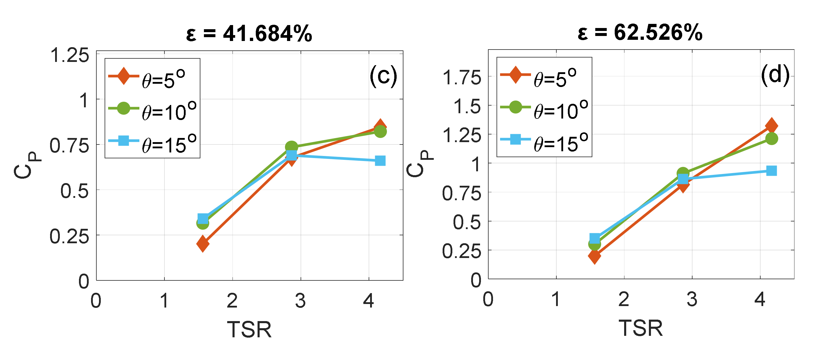
Figure 8.
Change in CP with varying the TSR and θ plotted at different ε of (a) 4.168%, (b) 20.842%, (c) 41.684%, and (d) 62.526% for rotor with the highest solidity (σ = 0.191).
Figure 8.
Change in CP with varying the TSR and θ plotted at different ε of (a) 4.168%, (b) 20.842%, (c) 41.684%, and (d) 62.526% for rotor with the highest solidity (σ = 0.191).


Figure 9.
Effect of θ on how ε alters CP of the highest solidity rotor (σ = 0.191) operating at different TSRs of (a) 1.563, (b) 2.865, and (c) 4.167.
Figure 9.
Effect of θ on how ε alters CP of the highest solidity rotor (σ = 0.191) operating at different TSRs of (a) 1.563, (b) 2.865, and (c) 4.167.

Figure 10.
Surface streamlines on the suction side of the highest solidity rotor (σ = 0.191) operating at TSR = 2.865: (a) ε = 20.842% & θ = 5°, (b) ε = 20.842% & θ = 15°, (c) ε = 62.533% & θ = 5°, and (d) ε = 62.533 & θ = 15°.
Figure 10.
Surface streamlines on the suction side of the highest solidity rotor (σ = 0.191) operating at TSR = 2.865: (a) ε = 20.842% & θ = 5°, (b) ε = 20.842% & θ = 15°, (c) ε = 62.533% & θ = 5°, and (d) ε = 62.533 & θ = 15°.

Figure 11.
Effect of TSR on how ε alters CP of the highest solidity rotor (σ = 0.191) that pitched to different θ values of (a) 5°, (b) 10°, and (c) 15°.
Figure 11.
Effect of TSR on how ε alters CP of the highest solidity rotor (σ = 0.191) that pitched to different θ values of (a) 5°, (b) 10°, and (c) 15°.

Figure 12.
Effect of σ on how ε alters CP at: (a) TSR = 2.865 & θ = 5°, (b) TSR = 2.865 & θ = 10°, (c) TSR = 2.865 & θ =15°, (d) TSR = 4.167 & θ = 5°, (e) TSR = 4.167 & θ = 10°, and (f) TSR = 4.167 & θ = 15°.
Figure 12.
Effect of σ on how ε alters CP at: (a) TSR = 2.865 & θ = 5°, (b) TSR = 2.865 & θ = 10°, (c) TSR = 2.865 & θ =15°, (d) TSR = 4.167 & θ = 5°, (e) TSR = 4.167 & θ = 10°, and (f) TSR = 4.167 & θ = 15°.

Figure 13.
The main effects of factors’ levels on the response variables (a) ∆CP, and (b) ∆CT.


Table 1.
Geometrical dimensions and operational specifications.
| Geometry/Operation Type | Specification |
|---|---|
| Hydrofoil | Eppler 395 |
| Number of blades (N) | 3 blades |
| Rotor radius (R) | 15.557 cm (6.125 in.) |
| Chord length (c) | 1.676, 3.81, 6.35 cm (0.66, 1.5, 2.5 in.) |
| Rotor solidity () | 0.0504, 0.115, 0.191 |
| Pitch angle (θ) | 5°, 10°, 15°, |
| Flow domain circular cross-section radius | 0.197, 0.241, 0.341, 0.762 m (7.746, 9.487, 13.416, 30 in.) |
| Flow velocity (U) | 1.5 m/s |
Table 2.
Independent variables with their magnitudes.
| Levels | Parameters | |||
|---|---|---|---|---|
| ε (%) | TSR | |||
| Low | 20.842 | 0.0504 | 5 | 1.563 |
| Medium | 41.684 | 0.115 | 10 | 2.865 |
| High | 62.533 | 0.191 | 15 | 4.167 |
Table 3.
Analysis of variance table for the effects of selected parameters on the ∆CP.
| Source | Degrees of Freedom | Adjusted Sum of Squares | Adjusted Mean Squares | F-Value | p-Value |
|---|---|---|---|---|---|
| Model | 64 | 4.501 | 0.070 | 52.55 | 1.363 × 10⁻¹¹ |
| Linear | 8 | 2.974 | 0.372 | 277.74 | 1.100 × 10⁻¹⁵ |
| 2 | 1.454 | 0.727 | 543.22 | 2.000 × 10⁻¹⁵ | |
| ε (%) | 2 | 0.360 | 0.180 | 134.43 | 9.905 × 10⁻¹¹ |
| θ (°) | 2 | 0.015 | 0.007 | 5.58 | 0.015 |
| TSR | 2 | 1.145 | 0.572 | 427.73 | 1.290 × 10⁻¹⁴ |
| 2-Way Interactions | 24 | 1.253 | 0.052 | 39.02 | 4.059 × 10⁻¹⁰ |
| *ε (%) | 4 | 0.283 | 0.071 | 52.95 | 5.001 × 10−09 |
| *θ (°) | 4 | 0.050 | 0.013 | 9.40 | 4.163 × 10−04 |
| *TSR | 4 | 0.593 | 0.148 | 110.78 | 1.898 × 10⁻¹¹ |
| ε (%)*θ (°) | 4 | 0.002 | 0.000 | 0.35 | 0.838 ** |
| ε (%)*TSR | 4 | 0.266 | 0.067 | 49.77 | 7.879 × 10−09 |
| θ (°)*TSR | 4 | 0.058 | 0.015 | 10.89 | 1.858 × 10−04 |
| 3-Way Interactions | 32 | 0.274 | 0.009 | 6.40 | 1.379 × 10−04 |
| *ε (%)*θ (°) | 8 | 0.008 | 0.001 | 0.79 | 0.623 ** |
| *ε (%)*TSR | 8 | 0.178 | 0.022 | 16.61 | 2.178 × 10−06 |
| *θ (°)*TSR | 8 | 0.074 | 0.009 | 6.88 | 5.595 × 10−04 |
| ε (%)*θ (°)*TSR | 8 | 0.014 | 0.002 | 1.34 | 0.295 ** |
| Error | 16 | 0.021 | 0.001 | ||
| Total | 80 | 4.523 |
** Statistically insignificant.
Table 4.
Analysis of variance table for the effects of selected parameters on the ∆CT.
| Source | Degrees of Freedom | Adjusted Sum of Squares | Adjusted Mean Squares | F-Value | p-Value |
|---|---|---|---|---|---|
| Model | 64 | 10.661 | 0.167 | 58.46 | 5.916 × 10⁻¹² |
| Linear | 8 | 7.858 | 0.982 | 344.72 | 2.000 × 10⁻¹⁶ |
| 2 | 5.230 | 2.615 | 917.72 | 0.000 | |
| ε (%) | 2 | 1.158 | 0.579 | 203.11 | 4.253 × 10⁻¹² |
| θ (°) | 2 | 0.333 | 0.167 | 58.44 | 4.420 × 10−08 |
| TSR | 2 | 1.138 | 0.569 | 199.60 | 4.863 × 10⁻¹² |
| 2-Way Interactions | 24 | 2.325 | 0.097 | 34.00 | 1.169 × 10−09 |
| *ε (%) | 4 | 0.892 | 0.223 | 78.26 | 2.691 × 10⁻¹⁰ |
| *θ (°) | 4 | 0.384 | 0.096 | 33.72 | 1.303 × 10−07 |
| *TSR | 4 | 0.533 | 0.133 | 46.76 | 1.245 × 10−08 |
| ε (%)*θ (°) | 4 | 0.057 | 0.014 | 4.96 | 0.009 |
| ε (%)*TSR | 4 | 0.263 | 0.066 | 23.07 | 1.776 × 10−06 |
| θ (°)*TSR | 4 | 0.197 | 0.049 | 17.24 | 1.187 × 10−05 |
| 3-Way Interactions | 32 | 0.477 | 0.015 | 5.23 | 4.933 × 10−04 |
| *ε (%)*θ (°) | 8 | 0.066 | 0.008 | 2.87 | 0.034 |
| *ε (%)*TSR | 8 | 0.174 | 0.022 | 7.65 | 3.065 × 10−04 |
| *θ (°)*TSR | 8 | 0.196 | 0.024 | 8.58 | 1.553 × 10−04 |
| ε (%)*θ (°)*TSR | 8 | 0.042 | 0.005 | 1.84 | 0.143 ** |
| Error | 16 | 0.046 | 0.003 | ||
| Total | 80 | 10.707 |
** Statistically insignificant.
Publisher’s Note: MDPI stays neutral with regard to jurisdictional claims in published maps and institutional affiliations. |
© 2022 by the authors. Licensee MDPI, Basel, Switzerland. This article is an open access article distributed under the terms and conditions of the Creative Commons Attribution (CC BY) license (https://creativecommons.org/licenses/by/4.0/).
Share and Cite
MDPI and ACS Style
Abutunis, A.; Menta, V.G. Comprehensive Parametric Study of Blockage Effect on the Performance of Horizontal Axis Hydrokinetic Turbines. Energies 2022, 15, 2585. https://doi.org/10.3390/en15072585
AMA Style
Abutunis A, Menta VG. Comprehensive Parametric Study of Blockage Effect on the Performance of Horizontal Axis Hydrokinetic Turbines. Energies. 2022; 15(7):2585. https://doi.org/10.3390/en15072585
Chicago/Turabian StyleAbutunis, Abdulaziz, and Venkata Gireesh Menta. 2022. "Comprehensive Parametric Study of Blockage Effect on the Performance of Horizontal Axis Hydrokinetic Turbines" Energies 15, no. 7: 2585. https://doi.org/10.3390/en15072585
Note that from the first issue of 2016, this journal uses article numbers instead of page numbers. See further details here.