
An Analytical Heat Transfer Model in Oil Reservoir during Long-Term Production


1
Department of Petroleum Engineering, Texas A&M University, College Station, TX 77843, USA
2
Department of Energy Resources Engineering, Stanford University, Stanford, CA 94305, USA
*
Author to whom correspondence should be addressed.
Energies 2022, 15(7), 2544; https://doi.org/10.3390/en15072544
Submission received: 21 February 2022
/
Revised: 28 March 2022
/
Accepted: 29 March 2022
/
Published: 31 March 2022
(This article belongs to the Section H1: Petroleum Engineering)
Abstract
:Contrary to the assumption of previous researchers, the radial temperature in the petroleum reservoir during production is non-isothermal because several heat transfer mechanisms change the radial temperature in reservoirs. As there have been few studies, especially after long-term production, this work derives steady-state analytic solutions considering the long-term production. It also presents sensitivity analysis with the various production conditions to investigate heat transfer between the producing fluids and surrounding formations during fluids flowing (hereafter, system heat transfer) in a steady-state. For oil production, the system heat transfer induces a cooling effect on the radial temperature in the reservoir, reducing the temperature rise due to the Joule–Thomson (J–T) heating. This cooling effect increases with the larger Peclet number, however, the relative contribution of the cooling effect to the radial temperature change diminishes. The equations explain that the cooling effect is proportional to the temperature increase due to J–T heating. With a larger permeability, a more convective-dominant phase causes more heat transfer actively. Although the cooling effect itself is amplified with the larger permeability, its relative contribution to the temperature change decreases. From the analysis, the cooling effect of system heat transfer is significant in the low-permeability reservoirs with large drawdown. The system heat transfer is confirmed to be an essential factor in measuring the accurate productivity index of unconventional reservoirs.
1. Introduction
Most of the early investigators have assumed the fluid temperature in a reservoir is isothermal because the Joule–Thomson (J–T) coefficient is negligible compared to the specific heat of fluids [1]. Early studies modeled only heat conduction and convection as the primary heat transfer mechanisms in the isothermal reservoir [2,3,4,5]. However, this assumption of the constant fluid temperature during a flow may not be applicable to many modern wells, such as deep-water reservoirs with significant pressure drawdowns [6,7,8]. Steffensen and Smith introduced the pioneer study to discuss the influence of J–T cooling and heating on temperature interpretations [9]. They showed J–T heating occurred in water injection wells, and J–T cooling was observed in gas wells. Data from the 81 drill stem tests in the North Sea by Hermanrud et al. supported their findings [10]. Based on the equations of state, Kortekaas et al. represented the temperature increase of 10–30 °C during gas condensate production from the high-pressure-high-temperature reservoirs [11]. App demonstrated the significant J–T heating effect in their field examples with the high drawdown condition [12]. Therefore, it is crucial to model the fluid temperature with the J–T heat transfer mechanism during oil and gas production.
The numerical hydrothermal simulation model has been applied to analyze the reservoir temperature through the conduction and convection mechanisms but without the J–T effect [13,14,15]. App developed a transient numerical model to consider all heat transfer mechanisms in the reservoir, including the J–T effect, adiabatic expansion, and heat transfer (H.T.) with the over- and under-burden formations [16]. He emphasized considering fluid property variations due to J–T heating (or cooling) which can affect well productivity. Ramazanov et al. proposed a numerical model accounting for the convection, radial heat conduction and the J–T effect [17]. Their model showed the J–T effect dominates the heat transfer during the constant rate-control production, while the impact of the radial conduction on the fluid temperature is minimal. This result is consistent with Steffensen and Smith’s description; the radial conduction is usually insignificant during production while the J–T effect acts as the primary heat transfer mechanism [9,17].
While the numerical analysis is applicable to various simulation conditions, the computational cost increases with a highly refined simulation grid and a small time step. With modeling assumptions such as homogeneity or isotropy, many authors have proposed analytical models to analyze the effects of the heat transfer mechanisms in the reservoirs during oil and gas production [18,19,20,21,22,23,24,25,26,27,28,29]. Onur and Cinar, and Mao and Zeidouni presented a transient analytical solution considering the J–T effect and adiabatic expansion but neglected vertical heat exchange with over- and under-burden formations [18,19,20,21,22]. Additionally, Mao and Zeidouni involved the near-wellbore damage in their transient analytical solution [20,21,22]. Based on Onur and Cinar’s analytical solution, Galvao et al. proposed a transient temperature model with pressure build-up [23]. Panini et al. extended Onur and Cinar’s model into the two-zone reservoir [24]. Mathias et al. derived a transient solution with the assumption of negligible radial conduction [25]. Chevarunotai proposed a transient analytical formulation with heat exchange into surrounding formations [26]. Hashish and Zeidouni also presented a transient analytical model with the surrounding heat exchange into multiple layers but neglected the J–T effect [27]. For a steady-state, App and Yoshioka proposed an analytical solution with the convection, conduction and the J–T effect, but they ignored the heat exchange into surroundings as well [28,29].
These numerical and analytical solutions have been used to demonstrate the impact of the J–T effect on the reservoir temperature during oil and gas production. App revealed that the J–T effect is the dominant factor in determining the temperature in the near-wellbore region with the immense pressure difference [16]. App and Yoshioka represent the temperature sensitivity with respect to the J–T effect in a dimensionless form [28]. They demonstrated that the larger J–T expansion leads to a higher fluid temperature in the oil reservoir. Another noteworthy finding is the temperature sensitivity analysis with respect to the Peclet number (Pe) which represents the heat transfer ratio of convection to conduction:
where is the local velocity, is the characteristic length, and is the thermal diffusivity. They showed that the influence of the Peclet number on the fluid temperature change is significant under the condition . In contrast, the impact of the Peclet number becomes minimized where the Peclet number is more than 1000 (i.e., the effect of convection is 1000 times greater than that of the conduction). Moreover, Xu highlighted that J–T heating could occur even in the gas reservoirs at specific pressure ranges [1]. This paper showed the J–T effect induces heating in the gas reservoirs when the pressure is higher than 10,000 psia.
Another noting finding is the impact of the heat transfer between the target reservoir and its surrounding formations. This heat transfer mechanism across the system boundary is “system heat transfer” for clarity in this work. As the reservoir fluid reaches the wellbore, a part of the heat energy from the J–T effect is dissipated into the surroundings (over- and under-burden formations). Chevarunotai pointed out that if the vertical heat exchange with over- and under-burden formations is neglected, significant temperature estimation error can occur, especially in the long-term production; the lack of heat loss into the surrounding formations overestimates the fluid temperature [26].
As conventional oil and gas production has been usually continued for several years [30,31,32,33], it is essential to analyze the steady-state physics with the J–T effect and the system heat transfer during the long-term production. This paper suggests three steady-state analytical solutions for hydrothermal modeling with the J–T effect. At first, we revisit a steady-state solution consistent with the dimensionless formulation proposed by App and Yoshioka [4]. In addition, we will demonstrate a more simplified version of a steady-state solution without radial conduction, which can be utilized at the low Peclet number. As the first two solutions are lacking heat transfer into the surrounding formations, we derive a new steady-state analytical solution that considers the surrounding heat transfer. Table 1 depicts the heat transfer processes considered in the previous studies and this work. Then, we demonstrate sensitivity analysis with respect to the Peclet number varied by production rate and permeability. We also represent the influence of the heat transfer between surrounding formations with the two suggested analytical solutions.
2. Mathematical Models
2.1. Analytical Steady-State Model without System Heat Transfer
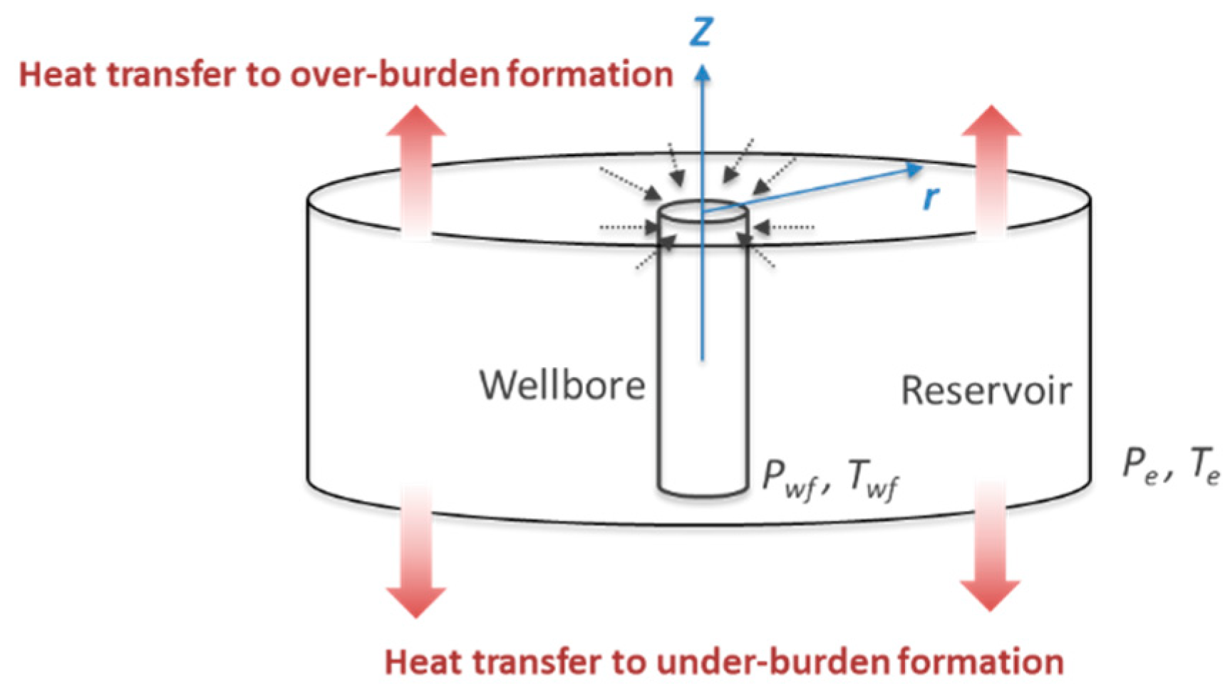
A single-phase fluid flows with no irreducible saturation from the outer reservoir boundary (re) toward the wellbore, as illustrated in Figure 1. The underlying assumptions in the model are: (1) Oil is the only flowing fluid in the reservoir (i.e., no free gas) and flows at a constant rate; (2) the fluid and formation temperature (Te) and pressure (Pe) in the reservoir are fixed as constant at the reservoir boundary; (3) all reservoir properties, such as porosity () and permeability (), are homogeneous, isotropic, and constant throughout the flow period; (4) the fluid density () and viscosity in the reservoir are constant.
The steady-state energy equation for this system considers the conservation of mass and energy. The comprehensive energy-balance equation for this system can be written to this partial-differential equation:
where is the saturation, is the fluid specific heat capacity, is the time, is the fluid velocity, is the Joule–Thomson throttling coefficient, is the fluid thermal conductivity, and subscripts f, wat, and e refer to the fluid, water and earth (formation), respectively. Here, is the net heat transfer between reservoirs which is assumed to be zero in this case. In Equation (2), the first and fourth terms on the left side are time-dependent and, thus, can be omitted because the steady-state is assumed. Since oil is the only fluid in the system, the subscript f can be replaced by o (oil), yielding Equation (3):
Equation (2) is the simplified, comprehensive energy-balance equation for the steady-state system. The terms on the left side of Equation (2) represent convection and energy change due to the J–T effect. The term on the right describes the change in energy from radial heat conduction. The volumetric flow rate, q, can be obtained from Darcy’s equation as follows:
where A is the cross-sectional area and h is the pay-zone height. The fluid velocity, , can be expressed, then,
Substituting Equations (4) and (5) to Equation (3), the second-order ODE form reads:
Arranging the above equation, the final form of the energy-balance equation can be the following second-order ordinary differential equation.
The two BCs are: (1) the initial temperature at the outer reservoir boundary; (2) thermal insulation at the wellbore wall:
The final form of the analytical solution is:
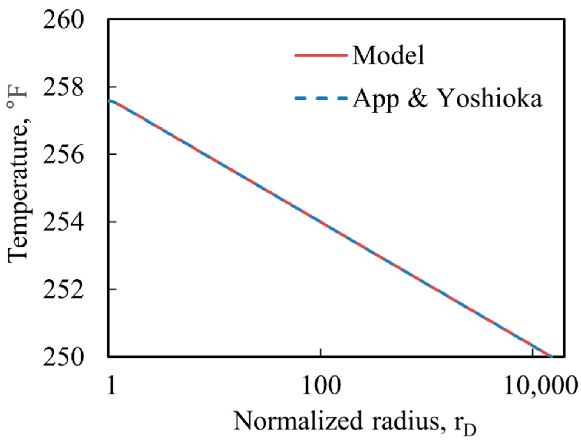
The analytic dimensional solution is compared with App and Yoshioka’s dimensionless solution to check consistency between the two solutions [28]. For the exact comparison, the same reservoir fluid and static properties data in their work are given in Table 2. The fluid conductivity is assumed as a single value to model conduction within the fluid and formation. Moreso, note that the fluid density value is evaluated at initial reservoir conditions. The variations of the J–T throttling coefficient are negligible, considering the pressure and temperature range in this work.
Figure 2 shows the comparison result. The derived model shows a consistent result with App and Yoshioka’s dimensionless solution, where the temperature difference between the two models is less than 0.1% throughout the whole dimensionless radial distance .
2.2. Analytical Steady-State Model without System Heat Transfer and Conduction
The radial conduction is usually negligible in heat transfer analysis with the constant flow injection or production rates [9,17,26]. With the insignificant conduction, Equation (7) is reduced to:
where we deploy the constants C and D in Equations (11) and (12). With the same boundary conditions in Equations (8) and (9), the reservoir temperature is derived as:
which is consistent with Mathias et al.’s analytical transient solution at [12]. Here, one notable finding is that Equation (14) is shown as a simplified version of Equation (10). Equation (14) neglects the second term of Equation (10) which accounts for the radial conduction.
2.3. Analytical Steady-State Model with System Heat Transfer
The reservoir is non-isothermal during the production period due to various heat transfer mechanisms. The most influential mechanism is the J–T effect [2,5,19,21]. Due to the J–T heating in the oil well, the fluid temperature in the reservoir rises as it flows, and almost reaches the maximum value where the fluids exit to the wellbore. Other representative mechanisms for temperature estimation include adiabatic expansion and heat transfer from a reservoir into over- and under-burden formations. Xu reported that the effect of the adiabatic expansion is negligible compared to that of the system heat exchange with the surrounding formations [1].
Chevarunotai investigated the system heat transfer impact on the radial reservoir temperature distribution [26]. The system heat transfer is related to the surrounding formation in a complex manner. Therefore, this paper approximated the heat transfer term using Newton’s law of cooling:
where hc is the heat transfer coefficient and subscript s represents the surrounding. Chevarunotai observed a significant temperature difference when considering the system heat transfer in a high-drawdown oil reservoir [26]. This model demonstrated a maximum of a 10 °F temperature when applied to the well data from App [16]. To identify the effect of system heat transfer at the steady-state, we derive the system heat transfer steady-state analytical solution from Chevarunotai’s transient analytical solution. With the assumption of the fixed and hc, and the negligible radial conduction, Chevarunotai’s transient solution is the following:
where the constants E, F, G, M and H are defined as:
To extend this transient solution into the steady-state, we introduce a constant n:
This transient solution is expected to reach the steady-state as and, thus, . Then, the integration part of the second term in Equation (16) can be rewritten for the steady-state as follows:
Implementing the L’Hopital’s formula, the exponential integral part is reduced to:
Therefore, the second term on the side of the transient solution is omitted. The steady-state solution is:
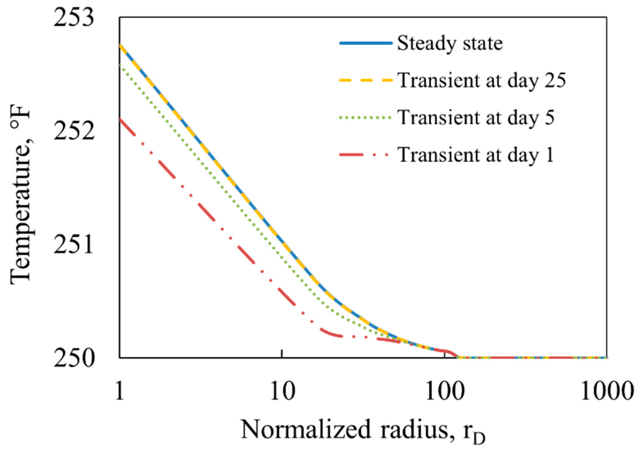
Using the data in Table 2, we evaluated three transient results on days 1, 5, and 25 with Equation (16) and the steady-state result with Equation (25). Figure 3 represents the convergence of transient results into the steady-state solution as time increases. This convergence pattern validates the accuracy of the derived steady-state solution.
3. Results
3.1. Identification of System Heat Transfer Effect
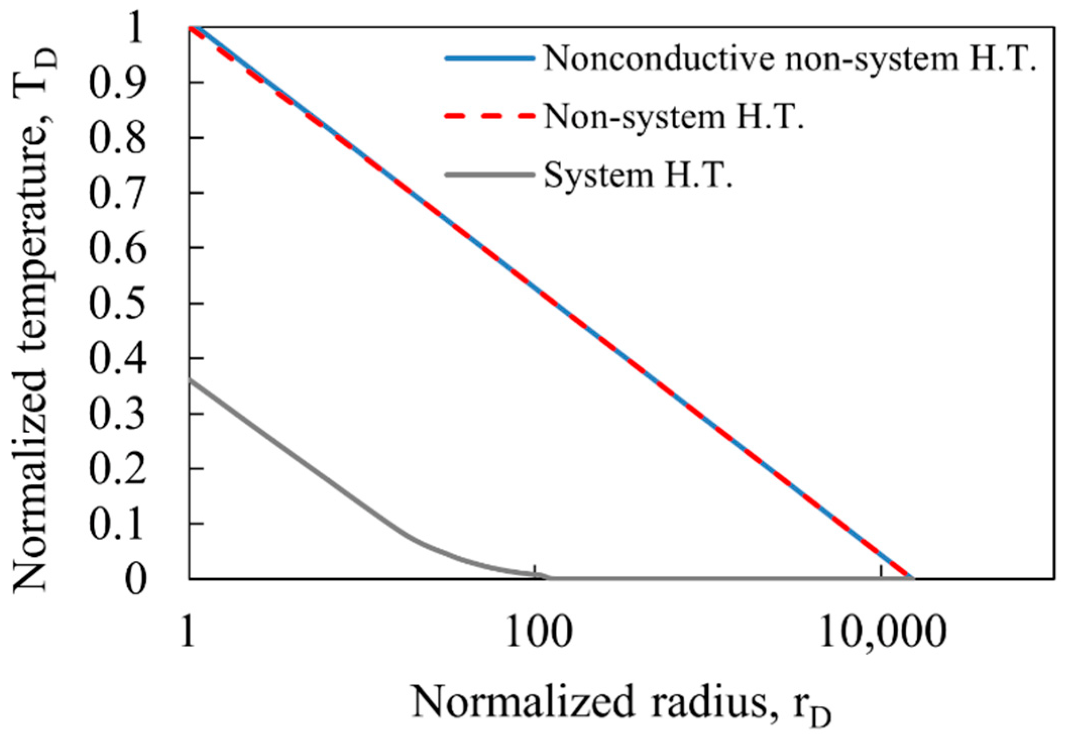
To identify the impact of system heat transfer, Table 3 presents the computed results by the three models: (1) the nonconductive non-system H.T. model in Equation (14), (2) the non-system H.T. model in Equation (10), and (3) the system H.T. model in Equation (25). The three models use the same reservoir and fluid heat properties presented in Table 2. Here, the production strategy is the constant rate control with 181.4 STB/day. The radius and temperature are dimensionless variables in Equations (26) and (27) where Tw is the wellbore wall temperature from the non-system H.T. model.
The reservoir fluid temperature increases as it approaches the wellbore radially due to the J–T effect. In this case, the most heating effect exists in the range from the wellbore to the radial distance of 350 ft (rD = 100). The estimated temperatures in this range are listed in Table 3. At first, the non-system H.T. model calculates the wellbore wall temperature (Tw) as 257.64 °F, which is 7.64 °F higher than the temperature at the outer boundary (Te) of 250 °F. This temperature increase is due to J–T heating, the most influential component in this system. Next, the conduction effect can be identified by comparing the non-system H.T. model with the nonconductive non-system H.T. model. The nonconductive non-system H.T. model computes 257.72 °F at the wellbore wall, which shows a very slight increase when compared with the result of the non-system H.T. model. This little temperature difference indicates that the effect of radial conduction is observable but minimal. Thus, the J–T effect is a dominant mechanism for rising up the temperature during production.
On the other hand, the system H.T. model shows 252.76 °F as the wellbore temperature, which is 2.76 °F higher than the outer boundary temperature. Compared with the temperature difference of 7.64 °F, calculated by the non-system H.T. model, the system H.T. model evaluates around 4.88 °F lower than that. The difference between the two models is due to the cooling effect of the system heat transfer, offsetting some portion of the temperature rise by J–T heating in the current oil-producing system. The system heat transfer cools down the reservoir temperature by dissipating the heat to the surrounding formations.
To identify the contribution of each heat transfer mechanism to the temperature change, the graph in Figure 4 uses the normalized parameters in Equations (26) and (27). The three curves in Figure 4 represent the normalized radial temperature for the logarithmic normalized radius. The system H.T. model indicates a cooler temperature profile than the other two models over the radial distance. Compared to the temperature at the wellbore wall by the non-system H.T. model, the system H.T. model shows a 35% temperature increase from the outer reservoir boundary. It means that the system heat transfer cools down around 65% of the total temperature rise due to J–T heating.
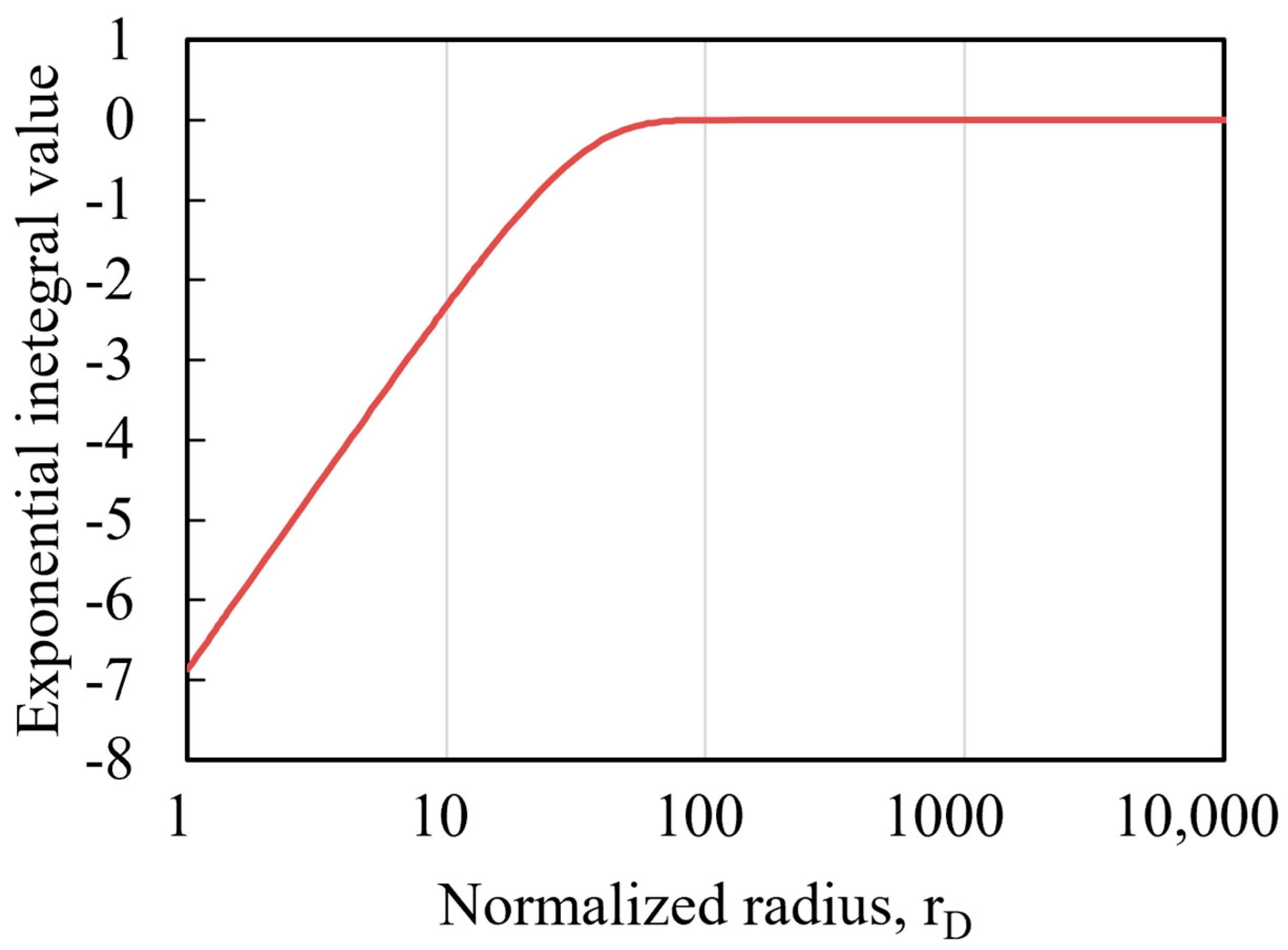
A key observation in Figure 4 is that the system H.T. model converges to the initial reservoir temperature (Te) at a certain radial distance between the normalized radius from 100 to 1000. From a mathematical point of view, this is due to the characteristic of the exponential integral function that is valid only within a limited range. A component in the solution converges to zero when the input value is less than −1. Figure 5 illustrates the output according to the radial distance in the current system. The Ei function output in this system converges at a radial distance of less than 100 of the normalized radius (i.e., 35 ft).
The steady-state condition may require an infinite flow period to complete the heat diffusion. The thermal diffusivity of the formation is typically very small compared to its hydraulic diffusivity. With the insignificant thermal diffusivity, an extremely long flow period can be required to end transient heat diffusion (i.e., reaching the steady-state). During the long flow period, the exponential integral in the system H.T. model is valid only within a limited radius in the steady-state (Figure 5). Therefore, we compare the temperature values only within the range of the normalized radius value of 100.
3.2. Sensitivity Analysis
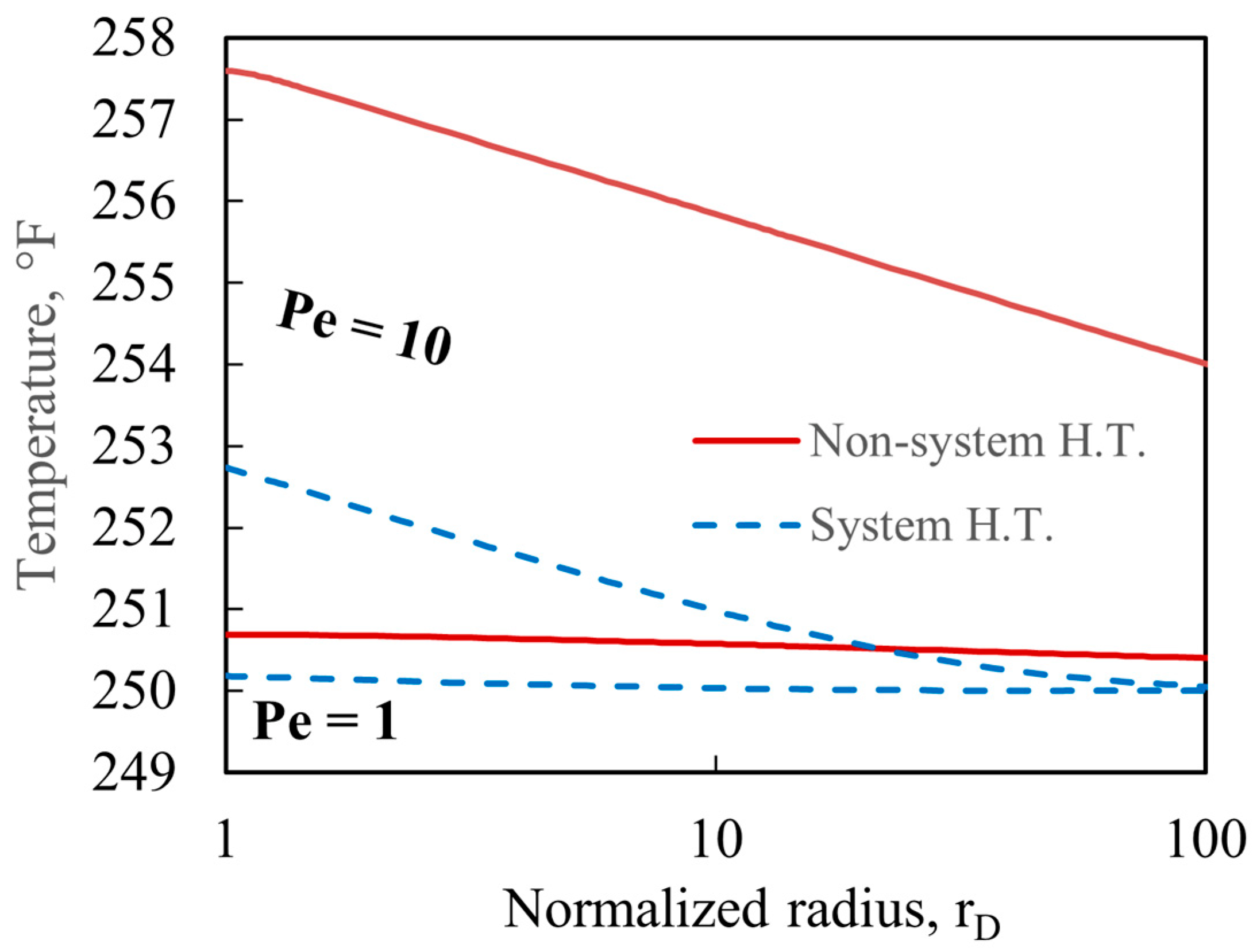
This section presents the sensitivity analysis of heat transfer parameters on temperature changes. From a physical standpoint, convection has a more significant heat transfer effect than conduction. Thus, the maximum temperature change can be shown when the convection occurs more dominantly. The Peclet number indicates the ratio of heat transfer by convection to heat transfer by conduction. Figure 6 illustrates the effect of each heat transfer mechanism with the varying Peclet numbers. The solid red line represents the radial temperature distribution computed by the non-system H.T. model, and the dotted blue line is derived from the system H.T. model. The Peclet numbers are 1 and 10, with corresponding flow rates of 18.1 STB/day and 181 STB/day, respectively.
In Figure 6, the magnitude of the system heat transfer can be interpreted as the radial temperature difference between the non-system H.T. model and the system H.T. model. When the Peclet number is one, the system heat transfer effect is minimal, less than 1 °F along with the whole radial distance. Meanwhile, when the Peclet number is 10, the effect becomes noticeable, as evidenced by the temperature difference at the wellbore wall of 4.5 °F. This is a reasonable result because this temperature difference from the J–T heating is proportional to the ratio of the two production flows. The bigger absolute effect is observed with the larger Peclet number.
From the drawdown, the J–T heating generates thermal energy, which can be transferred or/and distributed to a cooler region. The Peclet number is a ‘convection/conduction’ term, meaning the ratio of heat transfer is by convection to conduction. Because convection triggers J–T heating through the flow, the Peclet number indicates the amount of transferable thermal energy. As the Peclet number increases, the thermal energy generated by J–T heating and transferred by conduction is minimal because convection gradually dominates the whole heat transfer process. Conversely, the Peclet number converges to zero, implying that the thermal energy from the J–T heating is distributed or transferred by conduction. Due to the lower heat transfer speed of conduction than convection, the low Peclet number leads to the slow heat transfer and, thus, the smaller temperature increase. Thermodynamically, convection increases thermal internal energy with the J–T heating and kinetic energy with fluid flow. Therefore, the Peclet number is an effective measure to judge the degree of convection and energy increases.
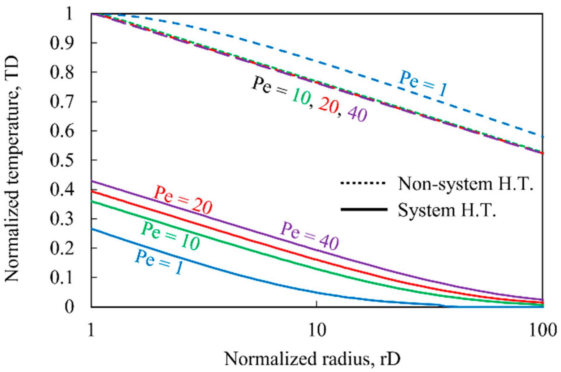
Figure 7 represents the relative contribution of system heat transfer by varying Peclet numbers 1, 10, 20, and 40. To show the relative contribution effectively, we normalize the temperature with respect to the wellbore wall temperature from the non-system H.T. model. When compared with the temperature at the wellbore wall (i.e., rD = 1), the system heat transfer induces around 73% of the total temperature rise when the Peclet number is one. A trend is observed that as the Peclet number increases, the relative cooling effect of the system heat transfer decreases. When the Peclet number is 40, the relative cooling effect is around 57% of the entire temperature change.
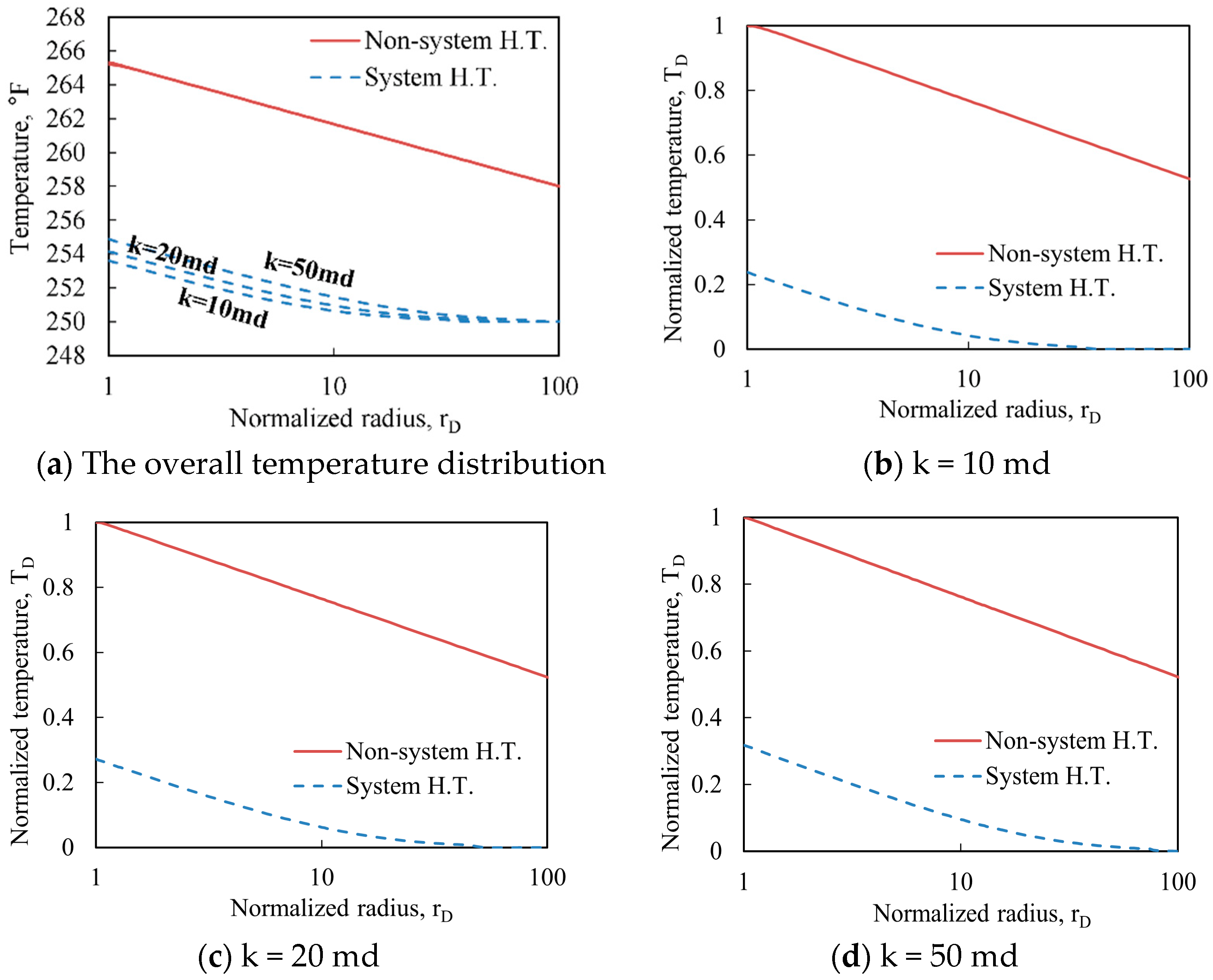
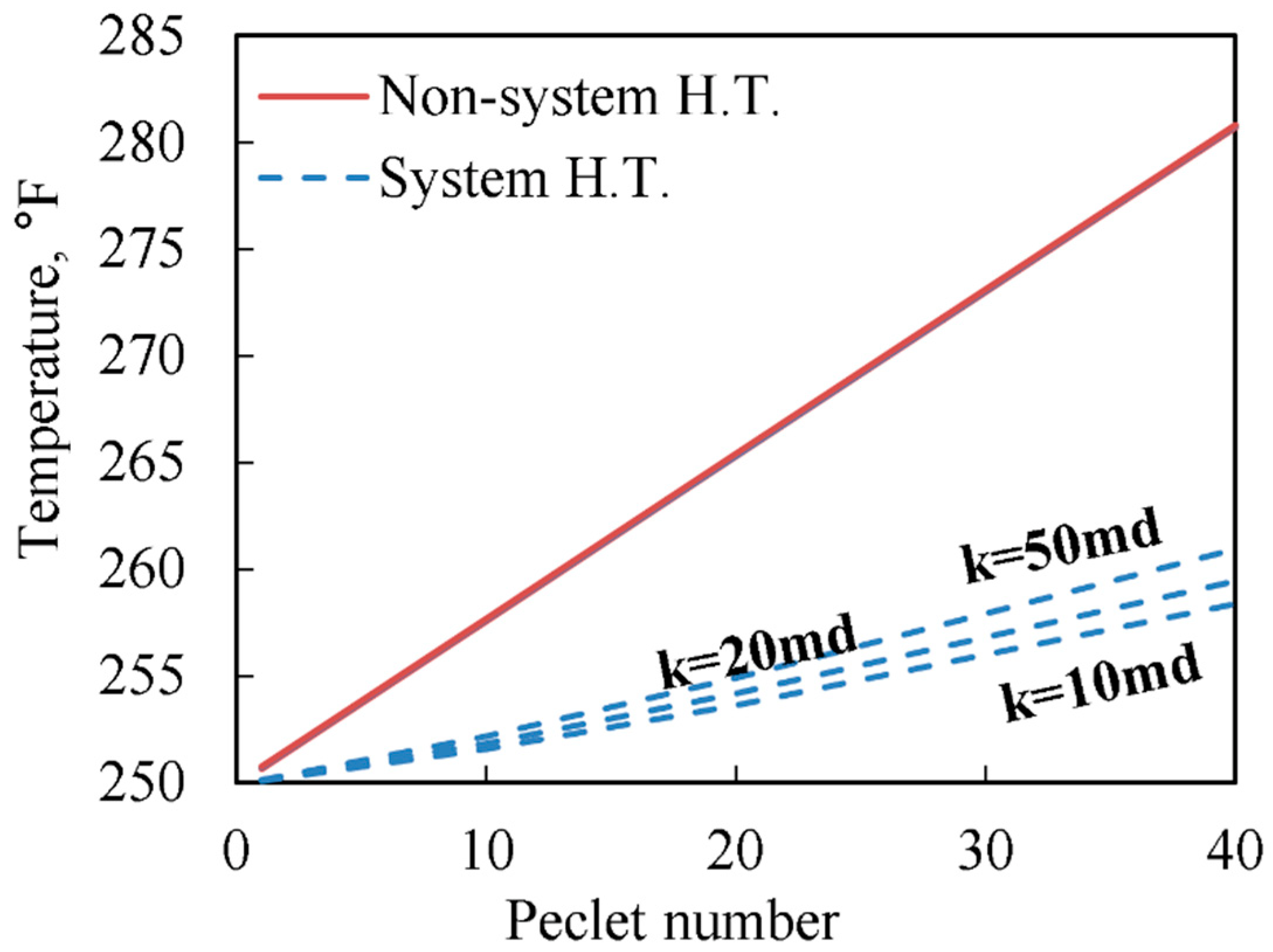
Figure 8 illustrates the radial temperature profiles of the two models with three different permeabilities. To ensure the same amount of pressure drawdown (i.e., a pressure difference between the wellbore and outer reservoir boundary), we adjust the production rate proportional to permeability: 90.5 STB/day, 181 STB/day, and 452.5 STB/day. The non-system H.T. model demonstrates almost the same radial temperature profiles regardless of the permeability difference (Figure 8a). The same drawdown condition here justifies little temperature difference among the three cases; the most contributing factor to the radial temperature change, J–T heating, is proportional to the drawdown. The slight temperature difference among the cases is observed mainly in the near-wellbore region (rD = 1). The only temperature difference near the wellbore indicates that the temperature change is primarily affected by other heat transfer mechanisms than the J–T effect.
On the other hand, the system H.T. model shows the different radial temperature profiles according to the permeability. Here, a bigger permeability leads to a higher radial temperature profile. Similar to the previous statement, the cooling effect of system heat transfer can be evaluated as the temperature difference between the non-system H.T. model and the system H.T. model. Therefore, less cooling impact from the system heat transfer is observed with the increased permeability.
In Figure 8b–d, we normalize the temperature to identify the relative contribution of the cooling effect from the system H.T. at each permeability. The relative contribution of the cooling effect diminishes as the permeability increases. Based on wellbore wall temperature, when the permeability is 10 md, the cooling effect is 76% of the entire radial temperature change. The relative ratio is lowered to 73% with the 20 md, and 68% with the 50 md. This observation for the relative contribution in Figure 8 is consistent with Figure 7. However, the absolute cooling effect shows a contrary trend between the two results. With the increasing Peclet number, Figure 6 demonstrates the rising absolute cooling effect while Figure 8 represents a decreasing absolute cooling effect. The Peclet number is proportional to the permeability (Equation (28)). The context of heat transfer can explain this observation. The higher Peclet number means that the convective heat transfer is more dominant over conduction. In the convective-dominant phase, the system heat loss is dissipated over the larger influx volume. This decreasing dissipation per unit fluid volume explains the lower relative contribution of system heat transfer at higher permeability.
Figure 9 describes the temperature change at the wellbore wall according to the Peclet number at different permeabilities. The temperature profiles of the non-system H.T. model show almost the same result in spite of the different Peclet numbers because of the same J–T heating, which is proportional to the pressure drawdown. On the contrary, the system H.T. model makes a slight difference in the temperature profiles according to the permeability, similarly to Figure 8a. As convection is dominant over conduction, the system heat loss is dissipated over the larger influx volume and, thus, drives to reduce the cooling effect.
Based on the aforementioned analysis, low permeability or/and high drawdown are the conditions in which the cooling effect of system heat transfer is significant. For example, tight oil is one of the representative unconventional resources featuring small permeability and a large drawdown for production. Predicting the temperature in these reservoirs without system heat transfer can lead to a significant error.
4. Discussion
Previous studies on reservoir heat transfer mainly focused on the temperature variation in the transient period, shown in Table 1. With the transient models, it is difficult to identify the effect of heat transfer mechanisms such as radial conduction and the system H.T. because the transient temperature update is mixed with other heat transfer processes. Moreover, because thermal diffusivity is usually much lower than hydraulic diffusivity, a few decades are required to reach the thermal steady-state: for example, about 13 years even in a small reservoir with 1500 ft of radius [34]. In this context, the previous transient models are not adequate tools for the steady-state due to the simulation with many time steps.
In this work, we presented two existing steady-state models without the system H.T.: one with conduction and the other without conduction. Then, we newly derived a steady-state model with the system H.T. The presented steady-state models can analyze each heat transfer process clearly after the long-term production by excluding the transient phenomena. Moreover, these models are computationally efficient because they require only one time step to reach the steady-state.
5. Conclusions
This study analyzed the contribution of heat transfer mechanisms influencing the radial temperature change in the oil reservoir during production. Key conclusions from this study are as follows:
- After long-term production and reaching a steady-state, a straight line is observed in the semi-log graph of radius and temperature.
- The system heat transfer induces a cooling effect on radial temperature in the oil reservoir, reducing some of the temperature rises due to J–T heating.
- As the Peclet number increases, the cooling effect of system heat transfer increases. However, its relative influence diminishes compared to J–T heating.
- Higher permeability causes the convection-dominating phase, which reduces the cooling effect of the system heat transfer.
Author Contributions
Conceptualization, M.J.; methodology, M.J. and J.A.; formal analysis, M.J., T.S.C. and J.A.; investigation, M.J.; writing—original draft preparation, M.J.; writing—review and editing, T.S.C. and J.A.; supervision, J.A. All authors have read and agreed to the published version of the manuscript.
Funding
This research received no external funding.
Institutional Review Board Statement
Not applicable.
Informed Consent Statement
Not applicable.
Data Availability Statement
The data presented in this study are available on request from the corresponding author.
Acknowledgments
We appreciate Rashid Hasan for his suggestions on this project.
Conflicts of Interest
The authors declare no conflict of interest.
Nomenclature
| J–T | Joule–Thomson |
| Pe | Peclet number |
| H.T. | heat transfer |
| STB | Barrel at the standard condition |
| A | cross-sectional area, |
| Formation volume factor, bbl/STB | |
| fluid specific heat capacity, Btu/(lbm·°F) | |
| h | pay-zone height, ft |
| heat transfer coefficient, Btu/(h··°F) | |
| permeability, md | |
| pressure, psi | |
| net heat transfer between reservoirs, Btu/(h·) | |
| q | volumetric well flow rate, STB/day |
| radius, ft | |
| saturation | |
| temperature, °F | |
| time, day | |
| fluid velocity, ft/day | |
| thermal diffusivity, /h | |
| fluid thermal conductivity, Btu/(h·ft·°F) | |
| viscosity, cp | |
| fluid density, lbm/ | |
| Joule-Thomson throttling coefficient, Btu/(lbm·psi) | |
| porosity | |
| Subscript | |
| D | dimensionless variable |
| earth (formation) | |
| f | fluid |
| o | oil |
| s | surrounding |
| w | well |
| wat | water |
| wellbore wall fluid |
References
- Xu, B. Modeling and Applications of Heat Transfer in Wellbore and Its Surrounding Formation. Ph.D. Thesis, Texas A&M University, College Station, TX, USA, 2018. [Google Scholar]
- Lauwerier, H.A. The Transport of Heat in an Oil Layer Caused by the Injection of Hot Fluid. Appl. Sci. Res. 1955, 5, 145–150. [Google Scholar] [CrossRef]
- Rubinshtein, L.I. The Total Heat Losses in Injection of a Hot Liquid into a Stratum. Neft’i Gaz 1959, 2, 41–48. [Google Scholar]
- Spillette, A.G. Heat Transfer during Hot Fluid Injection into an Oil Reservoir. J. Can. Pet. Technol. 1965, 4, 213–218. [Google Scholar] [CrossRef]
- Satman, A.; Brigham, W.E.; Zolotukhin, A.B. A New Approach for Predicting the Thermal Behavior in Porous Media during Fluid Injection. Trans. Geotherm. Resour. Counc. 1979, 3, 621–624. [Google Scholar]
- Sweet, M.L.; Sumpter, L.T. Genesis field, Gulf of Mexico: Recognizing Reservoir Compartments on Geologic and Production Time Scales in Deep-water Reservoirs. AAPG Bull. 2007, 91, 1701–1729. [Google Scholar] [CrossRef]
- Duan, S.; Lach, J.R.; Beadall, K.K.; Li, X. Water Injection in Deepwater, Over-Pressured Turbidites in the Gulf of Mexico: Past, Present, and Future. In Proceedings of the Offshore Technology Conference, Houston, TX, USA, 6–9 May 2013. [Google Scholar] [CrossRef]
- Dastkhan, Y.; Kazemi, A. The Impact of Isothermal Flow Assumption on Accuracy of Pressure Transient Analysis Results. Can. J. Chem. Eng. 2021, 1. [Google Scholar] [CrossRef]
- Steffensen, R.J.; Smith, R.C. The Importance of Joule-Thomson Heating (or Cooling) in Temperature Log Interpretation. In Proceedings of the Fall Meeting of the Society of Petroleum Engineers of AIME, Las Vegas, NV, USA, 30 September–3 October 1973. [Google Scholar] [CrossRef]
- Hermanrud, C.; Lerche, I.; Meisingset, K.K. Determination of Virgin Rock Temperature from Drillstem Tests. J. Pet. Technol. 1991, 43, 1126–1131. [Google Scholar] [CrossRef]
- Kortekaas, W.G.; Peters, C.J.; de Swaan Arons, J. Joule-Thomson Expansion of High-Pressure-High-Temperature Gas Condensates. Fluid Phase Equilib. 1997, 139, 205–218. [Google Scholar] [CrossRef]
- App, J.F. Field Cases: Nonisothermal Behavior Due to Joule-Thomson and Transient Fluid Expansion/Compression Effects. In Proceedings of the SPE Annual Technical Conference and Exhibition, New Orleans, LA, USA, 4–7 October 2009. [Google Scholar] [CrossRef]
- Naccache, P.F. A Fully-Implicit Thermal Reservoir. In Proceedings of the SPE Reservoir Simulation Symposium, Dallas, TX, USA, 8–11 June 1997. [Google Scholar] [CrossRef]
- Pao, W.K.S.; Lewis, R.W.; Masters, I. A Fully Coupled Hydro-Thermo-Poro-Mechanical Model for Black Oil Reservoir Simulation. Int. J. Numer. Anal. Meth. Geomech. 2001, 25, 1229–1256. [Google Scholar] [CrossRef]
- Yan, C.; Jiao, Y.; Yang, S. A 2D Coupled Hydro-Thermal Model for the Combined Finite-Discrete Element Method. Acta Geotech. 2019, 14, 403–416. [Google Scholar] [CrossRef]
- App, J.F. Nonisothermal and Productivity Behavior of High-Pressure Reservoirs. SPE J. 2010, 15, 50–63. [Google Scholar] [CrossRef]
- Ramazanov, A.S.; Nagimov, V.M.; Akhmetov, R.K. Analytical Model of Temperature Prediction for a Given Production History. Oil Gas Bus. 2013, 1, 537–546. [Google Scholar]
- Onur, M.; Çinar, M. Temperature Transient Analysis of Slightly Compressible, Single-Phase Reservoirs. In Proceedings of the 78th EAGE Conference and Exhibition, Vienna, Austria, 30 May–2 June 2016. [Google Scholar] [CrossRef]
- Onur, M.; Çinar, M. Analysis of Sandface-Temperature-Transient Data for Slightly Compressible, Single-Phase Reservoirs. SPE J. 2017, 22, 1134–1155. [Google Scholar] [CrossRef]
- Mao, Y.; Zeidouni, M. Accounting for Fluid-Property Variations in Temperature-Transient Analysis. SPE J. 2017, 23, 868–884. [Google Scholar] [CrossRef]
- Mao, Y.; Zeidouni, M. Analytical Solutions for Temperature Transient Analysis and Near Wellbore Damaged Zone Characterization. In Proceedings of the SPE Reservoir Characterisation and Simulation Conference and Exhibition, Abu Dhabi, United Arab Emirates, 8–10 May 2017. [Google Scholar] [CrossRef]
- Mao, Y.; Zeidouni, M. Transient and Boundary Dominated Flow Temperature Analysis under Variable Rate Conditions. In Proceedings of the SPE Trinidad and Tobago Section Energy Resources Conference, Port of Spain, Trinidad and Tobago, 25–26 June 2018. [Google Scholar] [CrossRef]
- Galvao, M.S.; Carvalho, M.S.; Barreto, A.B. A Coupled Transient Wellbore/Reservoir-Temperature Analytical Model. SPE J. 2019, 24, 2335–2361. [Google Scholar] [CrossRef]
- Panini, F.; Onur, M.; Viberti, D. An Analytical Solution and Nonlinear Regression Analysis for Sandface Temperature Transient Data in the Presence of a Near-Wellbore Damaged Zone. Transp. Porous Med. 2019, 129, 779–810. [Google Scholar] [CrossRef]
- Mathias, S.A.; Gluyas, J.G.; Oldenburg, C.M.; Tsang, C. Analytical Solution for Joule–Thomson Cooling during CO2 Geo-Sequestration in Depleted Oil and Gas Reservoirs. Int. J. Greenh. Gas Control. 2010, 4, 806–810. [Google Scholar] [CrossRef] [Green Version]
- Chevarunotai, N. Analytical Models for Flowing-Fluid Temperature Distribution in Single-phase Oil Reservoirs Accounting for Joule-Thomson Effect. Master’s Thesis, Texas A&M University, College Station, TX, USA, 2014. [Google Scholar]
- Hashish, R.G.; Zeidouni, M. Analytical Approach for Injection Profiling through Warm-Back Analysis in Multilayer Reservoirs. J. Pet. Sci. Eng. 2019, 182, 106274. [Google Scholar] [CrossRef]
- App, J.F.; Yoshioka, K. Impact of Reservoir Permeability on Flowing Sandface Temperatures: Dimensionless Analysis. SPE J. 2013, 18, 685–694. [Google Scholar] [CrossRef]
- App, J.F. Influence of Flow Geometry on Sandface Temperatures during Single-Phase Oil Production: Dimensionless Analysis. SPE J. 2016, 21, 928–937. [Google Scholar] [CrossRef]
- Anees, A.; Zhong, S.W.; Ashraf, U.; Abbas, A. Development of A Computer Program for Zoeppritz Energy Partition Equations and Their Various Approximations to Affirm Presence of Hydrocarbon in Missakeswal Area. Geosciences 2017, 7, 55–67. [Google Scholar] [CrossRef]
- Ashraf, U.; Zhang, H.; Anees, A.; Mangi, H.N.; Ali, M.; Zhang, X.; Imraz, M.; Abbasi, S.S.; Abbas, A.; Ullah, Z.; et al. A Core Logging, Machine Learning and Geostatistical Modeling Interactive Approach for Subsurface Imaging of Lenticular Geobodies in a Clastic Depositional System, SE Pakistan. Nat. Resour. Res. 2021, 30, 2807–2830. [Google Scholar] [CrossRef]
- Jiang, R.; Zhao, L.; Xu, A.; Ashraf, U.; Yin, J.; Song, H.; Su, N.; Du, B.; Anees, A. Sweet Spots Prediction through Fracture Genesis Using Multi-Scale Geological and Geophysical Data in the Karst Reservoirs of Cambrian Longwangmiao Carbonate Formation, Moxi-Gaoshiti Area in Sichuan Basin, South China. J. Petrol. Explor. Prod. Technol. 2021. [Google Scholar] [CrossRef]
- Ullah, J.; Luo, M.; Ashraf, U.; Pan, H.; Anees, A.; Li, D.; Ali, M.; Ali, J. Evaluation of the Geothermal Parameters to Decipher the Thermal Structure of the Upper Crust of the Longmenshan Fault Zone Derived from Borehole Data. Geothermics 2022, 98, 102268. [Google Scholar] [CrossRef]
- Palabiyik, Y.; Onur, M.; Tureyen, O.I.; Cinar, M. Transient Temperature Behavior and Analysis of Single-Phase Liquid-Water Geothermal Reservoirs during Drawdown and Buildup Tests: Part I. Theory, New Analytical and Approximate Solutions. J. Pet. Sci. Eng. 2016, 146, 637–656. [Google Scholar] [CrossRef]
Figure 1.
Schematic heat transfer of reservoir and formation where r is the radius from the wellbore, P_wf is the wellbore wall fluid pressure, T_wf is the wellbore wall fluid temperature.
Figure 1.
Schematic heat transfer of reservoir and formation where r is the radius from the wellbore, P_wf is the wellbore wall fluid pressure, T_wf is the wellbore wall fluid temperature.

Figure 2.
The comparison result of the radial temperature distribution between the two models; App and Yoshioka‘s model (blue) and our derived model (red).
Figure 2.
The comparison result of the radial temperature distribution between the two models; App and Yoshioka‘s model (blue) and our derived model (red).

Figure 3.
Transient and steady-state results with the system heat transfer.

Figure 4.
Comparison of the normalized radial temperature distribution among the three steady-state cases: the nonconductive non-system H.T. model, the non-system H.T. model, and the system H.T. model.
Figure 4.
Comparison of the normalized radial temperature distribution among the three steady-state cases: the nonconductive non-system H.T. model, the non-system H.T. model, and the system H.T. model.

Figure 5.
Exponential integral value throughout the reservoir radius.

Figure 6.
Comparison of radial temperature distribution with varying Peclet numbers.

Figure 7.
Comparison of system heat transfer at different Peclet numbers: Pe = 1 (blue); Pe = 10 (green); Pe = 20 (red); Pe = 40 (purple).
Figure 7.
Comparison of system heat transfer at different Peclet numbers: Pe = 1 (blue); Pe = 10 (green); Pe = 20 (red); Pe = 40 (purple).

Figure 8.
Comparison of radial temperature profiles of the two models at different permeability: (a) the overall temperature distribution: (b) k = 10 md; (c) k = 20 md; (d) k = 50 md.
Figure 8.
Comparison of radial temperature profiles of the two models at different permeability: (a) the overall temperature distribution: (b) k = 10 md; (c) k = 20 md; (d) k = 50 md.

Figure 9.
Wellbore wall temperature with Peclet number at different permeabilities.


Table 1.
Heat transfer mechanism of each model (AE: adiabatic expansion).
| Transient State | Steady-State | |
|---|---|---|
| App (2010) [16] | J–T, AE, System H.T. | |
| Mathias et al. (2010) [25] | J–T | |
| Ramazanov (2013) [17] | J–T, Radial conduction | |
| App and Yoshioka (2013) [28] | J–T, Radial conduction | |
| Chevarunotai et al. (2014) [26] | J–T, System H.T. | |
| Onur and Cinar (2016) [18,19] | J–T, AE | |
| Mao and Zeidouni (2017) [20,21,22] | J–T, AE | |
| Hashish and Zeidouni (2019) [27] | AE, System H.T. | |
| Our proposed model | J–T, System H.T. |
Table 2.
Well, formation, and fluid data (STB: barrel at the standard condition) [28].
Table 2.
Well, formation, and fluid data (STB: barrel at the standard condition) [28].
| Parameters | Value |
|---|---|
| , ft | 5325 |
| , ft | 0.35 |
| Pay-zone height, h, ft | 10 |
| 0.18 | |
| Permeability, k, md | 20 |
| , Btu/(h·°F·ft) | 1.93 |
| , lbm/ft3 | 51.19 |
| , Btu/(lbm·°F) | 0.53 |
| , cp | 1 |
| , Btu/(lbm·psi) | 0.00313 |
| , bbl/STB | 1.05 |
| Well flow rate, q, STB/day | 181.95 |
| , °F | 250 |
| , psi | 10,000 |
| ·°F) [26] | 0.92 |
Table 3.
Radial temperature results from the three steady-state models: the nonconductive non-system H.T. model, the non-system H.T. model, and the system H.T. model.
Table 3.
Radial temperature results from the three steady-state models: the nonconductive non-system H.T. model, the non-system H.T. model, and the system H.T. model.
| Radius, ft | rD | Temperature, °F Nonconductive Non-System H.T. | Temperature, °F Non-System H.T. | Temperature, °F System H.T. |
|---|---|---|---|---|
| 0.35 (=rw) | 1 | 257.72 | 257.64 | 252.76 |
| 3.5 | 10 | 255.87 | 255.84 | 250.99 |
| 35 | 100 | 254.03 | 254.03 | 250.06 |
| 350 | 1000 | 252.18 | 252.18 | 250.00 |
Publisher’s Note: MDPI stays neutral with regard to jurisdictional claims in published maps and institutional affiliations. |
© 2022 by the authors. Licensee MDPI, Basel, Switzerland. This article is an open access article distributed under the terms and conditions of the Creative Commons Attribution (CC BY) license (https://creativecommons.org/licenses/by/4.0/).
Share and Cite
MDPI and ACS Style
Jang, M.; Chun, T.S.; An, J. An Analytical Heat Transfer Model in Oil Reservoir during Long-Term Production. Energies 2022, 15, 2544. https://doi.org/10.3390/en15072544
AMA Style
Jang M, Chun TS, An J. An Analytical Heat Transfer Model in Oil Reservoir during Long-Term Production. Energies. 2022; 15(7):2544. https://doi.org/10.3390/en15072544
Chicago/Turabian StyleJang, Minsoo, Troy S. Chun, and Jaewoo An. 2022. "An Analytical Heat Transfer Model in Oil Reservoir during Long-Term Production" Energies 15, no. 7: 2544. https://doi.org/10.3390/en15072544
Note that from the first issue of 2016, this journal uses article numbers instead of page numbers. See further details here.