
Effects of Automated Vehicle Models at the Mixed Traffic Situation on a Motorway Scenario


1
Department of Control for Transportation and Vehicle Systems, Faculty of Transportation Engineering and Vehicle Engineering, Budapest University of Technology and Economics, Műegyetem rkp. 3., H-1111 Budapest, Hungary
2
Institute of Automotive Engineering, TU Graz, 8010 Graz, Austria
3
Institute of Highway Engineering and Transport Planning, TU Graz, 8010 Graz, Austria
*
Author to whom correspondence should be addressed.
Energies 2022, 15(6), 2008; https://doi.org/10.3390/en15062008
Submission received: 30 January 2022
/
Revised: 24 February 2022
/
Accepted: 7 March 2022
/
Published: 9 March 2022
(This article belongs to the Special Issue Advances in Automated Driving Systems)
Abstract
:There is consensus in industry and academia that Highly Automated Vehicles (HAV) and Connected Automated Vehicles (CAV) will be launched into the market in the near future due to emerging autonomous driving technology. In this paper, a mixed traffic simulation framework that integrates vehicle models with different automated driving systems in the microscopic traffic simulation was proposed. Currently, some of the more mature Automated Driving Systems (ADS) functions (e.g., Adaptive Cruise Control (ACC), Lane Keeping Assistant (LKA), etc.) are already equipped in vehicles, the very next step towards a higher automated driving is represented by Level 3 vehicles and CAV which show great promise in helping to avoid crashes, ease traffic congestion, and improve the environment. Therefore, to better predict and simulate the driving behavior of automated vehicles on the motorway scenario, a virtual test framework is proposed which includes the Highway Chauffeur (HWC) and Vehicle-to-Vehicle (V2V) communication function. These functions are implemented as an external driver model in PTV Vissim. The framework uses a detailed digital twin based on the M86 road network located in southwestern Hungary, which was constructed for autonomous driving tests. With this framework, the effect of the proposed vehicle models is evaluated with the microscopic traffic simulator PTV Vissim. A case study of the different penetration rates of HAV and CAV was performed on the M86 motorway. Preliminary results presented in this paper demonstrated that introducing HAV and CAV to the current network individually will cause negative effects on traffic performance. However, a certain ratio of mixed traffic, 60% CAV and 40% Human Driver Vehicles (HDV), could reduce this negative impact. The simulation results also show that high penetration CAV has fine driving stability and less travel delay.
1. Introduction
With the rapid development of autonomous driving technology, Autonomous Vehicles (AV) have entered the operational stage in the road transport system. It is foreseeable that, in the near future, the proportion of AV will gradually increase. However, extensive autonomous driving is still out of reach. Considering the enormous possession of conventional vehicles, the first possibility of autonomous driving to implement on the road is the mixed traffic flow. This possibility will first appear in the motorway scenario, which is much simpler than urban roads. The mixing of AV and conventional vehicles will definitely have a significant impact on the performance of motorway traffic.
AV refer to the vehicles that can achieve the environment perception, route planning, decision making, and vehicle control functions in a highly intelligent and safe manner through the advanced on-board sensors, controllers, and actuators. The Society of Automotive Engineers (SAE) divides autonomous driving into six levels from Level 0 to Level 5 according to the need of the amount of driver intervention [1]. Level 0–Level 2 are defined as Advance Driver Assistant System (ADAS) while Level 3–Level 5 are defined as high-level automatic driving system. As high-level autonomous vehicles carry massive electronic devices, they are usually based on electric vehicles [2,3]. Connected and Automated Vehicles (CAV) refer to autonomous vehicles with integrated communication systems and network technologies to realize intelligent information transfer, exchange, and sharing between vehicles and everything (other vehicles, transport infrastructure, passersby, clouds, etc.). CAV have the capability of complex environment perception, intelligent decision making, and collaborative control, which can realize safe, efficient, comfortable, and energy-saving driving.
In this paper, we mainly focus on the Highly Autonomous Vehicles (HAV) and CAV simulation where HAV are defined as autonomous vehicles with Level 3 automation technology introduced in [4]. Vehicles with increasing levels of automation will fuse information from on-board multi-sensors and systems, allowing the vehicle to perceive the surrounding traffic and to locate itself precisely. Meanwhile, systems can enable the piloting of the vehicle with little or no human intervention during highly automated driving. Furthermore, the CAV model in this paper refers to vehicles with dedicated short-range communication technologies based on highly automated driving function, which allows vehicles to communicate with their surroundings, including infrastructure and other vehicles. In addition, it can provide drivers with real-time information about road and traffic conditions, as well as a wide range of connectivity services.
According to the market forecast of [5], the share of HAV and CAV in new car sales will increase from about 10% in 2025 to about 50% in 2035. Therefore, it is particularly important to evaluate the existing traffic scenario, driven by the huge market prospect.
Vehicle automation and communication technologies are considered promising approaches to improve the efficiency, safety, and environmental protection of traffic systems. Numerous studies have investigated the impacts of autonomous vehicles on traffic with simulation technology. However, the current Traffic Analysis, Modeling, and Simulation (TAMS) tools are not adequate for evaluating CAV or HAV driving behavior. Changes of the driving behavior parameter even had the opposite effect in different microscopic traffic simulation tools [6]. The reasons for this are as follows. First, for the CAV model, most TAMS tools cannot simulate vehicle inter-connectivity, i.e., V2V communication information sharing. Additionally, the majority of driving models are unrealistic, and many existing models require parameter calibration. Refs. [7,8,9] introduce the approaches to use empirical data to calibrate Wiedemann 99 model in Vissim in order to replicate CAV and HAV driving behavior. This method requires much time for collecting road data, which reduce the cost of modeling but require a lot of effort in training the samples as well as data statistics. In addition, most of them did not systematically evaluate the lateral/longitudinal control model, and [10,11] apply a linearized ACC model to perform speed control while considering only the following distance. To real driving conditions, the driver’s desired speed should also be considered as a significant input to the system. Finally, Ref. [12] introduces HAV and CAV simulation models where control strategy is simplified. Although this approach reduces the difficulty of modeling, it does not reflect the actual vehicle driving behavior. In order to realistically reflect the driving behavior of HAV and CAV on the highway, we propose a driving model based on the Highway Chauffeur (HWC) function, which is introduced and defined in [13].
2. Methodology
For the HAV model, the proposed functionality (HWC) is defined as conditional automated driving function (SAE level 3—Conditional Automation) for standard driving, that is based on requirements and conditions defined by PEGASUS in [13]. PEGASUS is a research project which aims for a definition of a standardized procedure for the testing and experimenting of automated vehicle systems in simulation and real environments. Regarding the conditional automation on the guidance level, HWC function shall be capable of controlling the vehicle in longitudinal and lateral direction if the current vehicle state allows it. Additionally, the CAV model is defined by a lane change warning system on the basis of HWC, which ascertains the surrounding vehicle motion states based on V2V communication. The safe distance between ego vehicle and rear vehicle in the target lane is analyzed according to the goal of both collision avoidance and vehicle following safety.
2.1. Simulation Platform
Traffic analysis, modeling, and simulation is a mature field; several simulators are available. Each simulator has its own advantages in simulating real-world traffic based on a different car-following model. Typical TAMS tools applied by traffic engineers are PTV VISSIM [14], Simulation of Urban MObility (SUMO) [15], CORSIM [16], and Paramics [17]. Vissim is a microscopic road traffic simulator developed by PTV Group. Due to the comprehensive simulation diversity (motor vehicle module, bicycle module, pedestrian module, public transportation module, traffic timing module, etc.), as well as multi-dimension and efficiency of traffic simulation parameters, it is widely used in consulting firms, academia, and the public sector in the field of road traffic simulation.
Vissim provides a user-friendly Graphical User Interface (GUI), which means the user does not need to write programs manually to call different simulation modules and set up simulations. In addition to visual applications, Vissim also offers script-based modeling, which is very useful when users aim to dynamically access and control Vissim objects during simulation. This can be achieved through the COM (Component Object Model) interface, a technology that realizes inter-process communication between software with various programming language (e.g., C++, Phyton, Visual Basic, Java, Matlab, etc.).
The Vissim COM interface defines a hierarchical model with a head called IVissim, which represents the Vissim object. Under IVissim, there are different objects in which the functions and parameters of the simulator originally provided by the GUI can be controlled by programming. The Vissim-COM programming is introduced through Matlab Script for the co-simulation framework. For this Vissim-COM interface, [18] introduced a detailed development of the simulation environment. It is capable of performing all simulation sequences with the flexibility to allow the user to calibrate parameters and finally generate statistical plots automatically.
2.2. External Driving Model
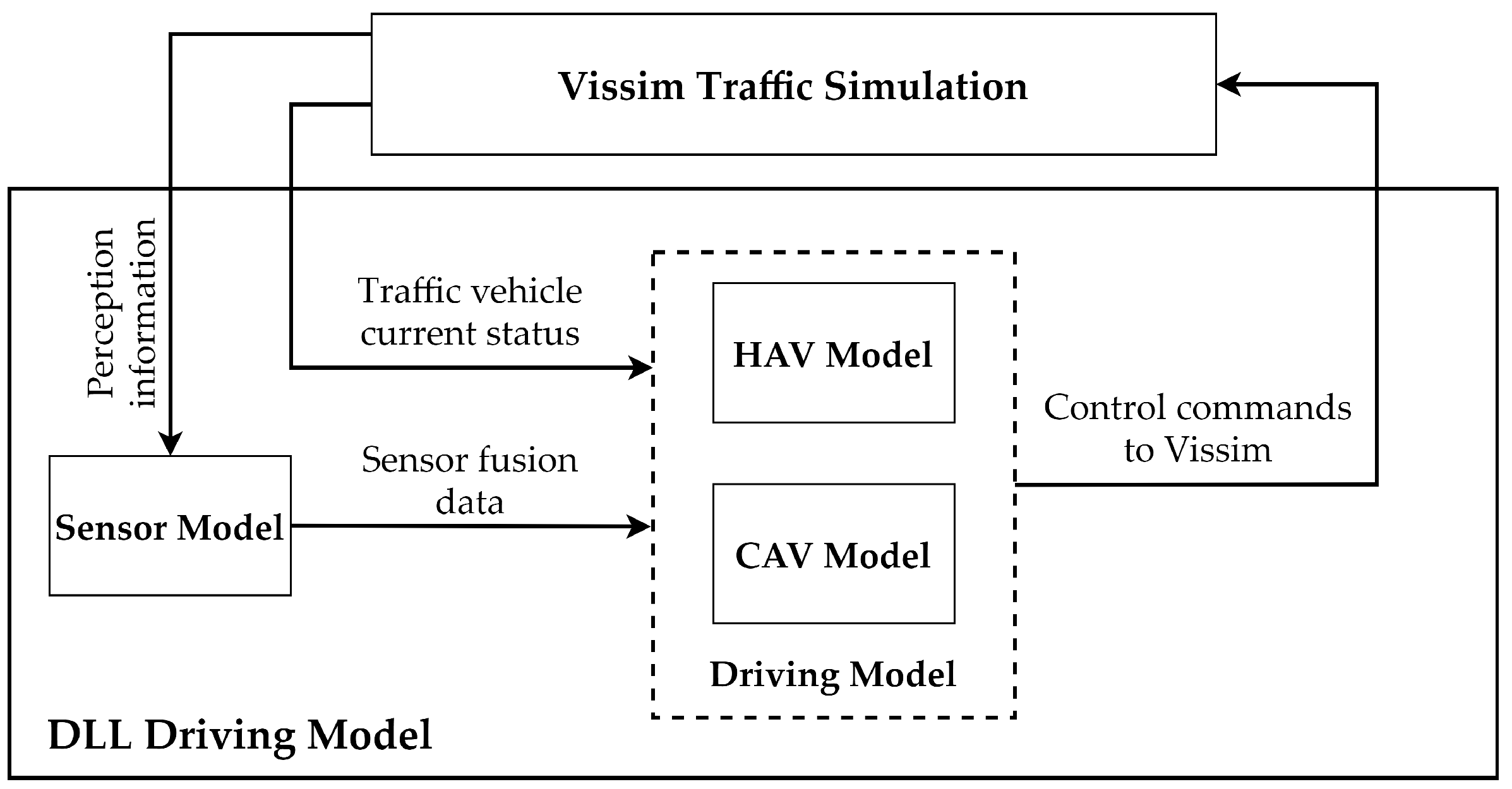
The models are implemented in Vissim described in [18,19] using the External Driving Model interface (DLL). This interface provides the possibility to implement driver models with defined driving behavior. Similar functions are available through a Python interface called Traffic Control Interface (TraCI) in SUMO [20]. The whole DLL driving model is illustrated in Figure 1, which consists of three models. Considering that the traffic participants in Vissim cannot individually set up a sensor model to perceive the surrounding obstacles, DLL provides a possibility to obtain specific parameters of the surrounding vehicles (e.g., relative distance and velocity, heading angle, etc.) passed from Vissim. As a consequence, this perception information is gathered in the sensor model then sent to the driving model (HAV and CAV) as input. In parallel, driving models receive sensor fusion data and current vehicle dynamics data from Vissim to calculate lateral and longitudinal control commands, which are fed back to Vissim and the movement of the traffic vehicle is completed in the loop. The three models are described in more detail in the following subsections.
2.3. Sensor Model
There are several different sensors built in a modern car supported to assist the driver or even drive autonomously. Therefore, the sensor model plays an important role in the adaptive control of the ego car and objects perception. Due to the limitations of Vissim, it is not possible to provide sensor models, a simplified sensor model is therefore presented here. In [21], an advanced driver assistance system is introduced from Toyota, which has been commercially realized in Japan in 2021. This system has multi-modal sensors covering the complete periphery of 360 degrees. Hence, the sensor model should have the ability to detect the surrounding objects, especially traffic participants upstream and downstream of the adjacent lane. Additionally, the most important parameter is to set the effective range of the sensor detection. Namely, only traffic participants within the detection range are considered. With the development of sensor technology, long-range radar is a range capability up to 150–200 m, presented in [22]. Therefore, a maximum detection range of 200 m is defined in the sensor model. The main function of the sensor model is to receive the specific parameters of the traffic participants from Vissim and transmit them to the driving function model by combining sensory data and fusion algorithms. Hence, Time to Collision (TTC), the lane change decision, and other perception signals are introduced in the subsequence.
2.3.1. Time to Collision Calculation
TTC is used to determine the time difference between the current time to a future moment when a potential crash will happen. It is a snapshot of the currently prevailing conditions and is only valid if the conditions stay stable. Nevertheless, it is useful for the prediction of potential crashes and for classifying the time-based safety distance to other traffic participants. The calculation of the TTC starts with the position of a car in dependency of the driving velocity, and the acceleration is described by Equation (1), where s and v are relative distance and velocity between ego and target car acquired from Vissim, respectively, and a is collected based on current ego car driving dynamics. The calculation of TTC t is therefore, the solution (Equation (2)) to Equation (1).
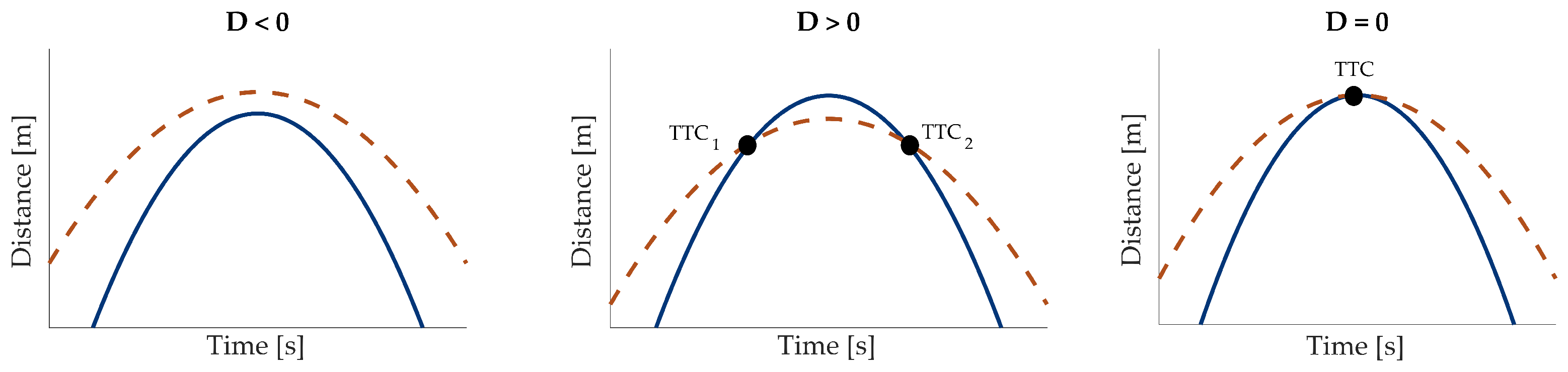
Decisive for the solution of the equation for is the term under the square root, also called determinant D in Equation (3). There are three possible cases shown in Figure 2.
- : there is no collision expected. For example, if a car is traveling behind another car with the same speed and both start braking at the same moment, but the ego car decelerates more than the target car so that a collision does not occur.
- : in comparison, if the ego vehicle decelerates much less than the target vehicle, a crash will theoretically happen at TTC1 and TTC2. Due to the quadratic function, there are two solutions, however, only one of them is valid as the other one is a theoretical moment in the past in most cases.
- : there is only one result for the TTC calculation.
When the TTC calculation is positive, it means that the velocity of the ego car is faster than that of the target car. Namely, the ego car is accelerating relative to the target car. Conversely, the TTC is negative, which means the ego car is decelerating relative to the target vehicle. In addition, the TTC is assumed to be the maximum value when there is no vehicle within the front detection distance or maintaining the same speed as the target car. Finally, When the TTC is towards zero, this is a very hazardous situation, meaning that the distance between vehicles is decreasing and a potential collision may occur. Therefore, TTC, as an important output of the sensor model, will be used as an essential condition to determine the occurrence of the lane change.
2.3.2. Decision Making
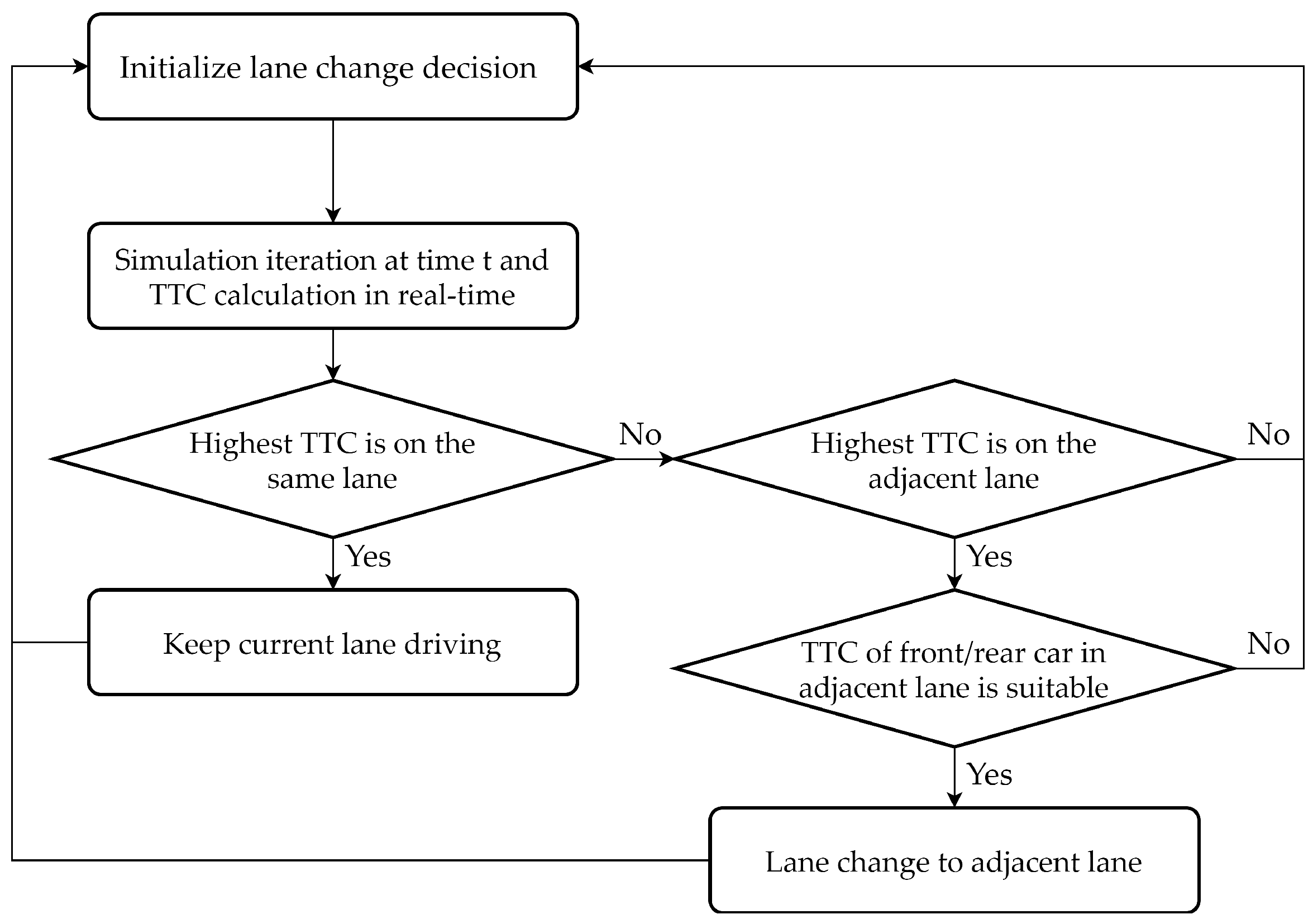
Decision making is another important function in the sensor model. In the previous section, TTC has been determined. The decision to change lanes based on the left-hand overtaking rule of the road is therefore initialized according to the TTC, which are predefined by the decision-making algorithm. Figure 3 illustrates a decision-making process to decide lane change direction. These commands will be as an internal signal transmitted to the driving function model. Before the vehicle reaches cruising speed, if the TTC detected in the same lane is highest, it means the target vehicle is far enough away to be safe. Therefore, the ego car can continue to drive on the current lane unless the adjacent lane TTC is higher and the lane change condition is satisfied; in this case, the sensor model will send a lane change decision signal to the driving model. Even during the lane change execution, the sensor model continues the TTC calculation between the surrounding cars in simulation iteration and the ego car in order to change the lane change decision at any time.
2.3.3. Other Relevant Signals
Other signals related to sensor sensing can be read directly from the Vissim simulation environment via the DLL interface, without additional computation. These signals will be used in the driving function model as well. These signals include:
- The relative speed, acceleration, and distance of the surrounding vehicles are used to adjust longitudinal and lateral control.
- Adjacent lane detection free space is used to determine lane change conditions.
- The position information of adjacent lanes for the multiple-lane road; according to the highway overtaking rules, overtaking on the right hand should be prohibited.
- For CAV, the sensor model is responsible for receiving the broadcasted V2V information and transmitting it to the control module.
2.4. Highly Automated Vehicle Model
The HAV model is implemented based on HWC function defined in [13], which is the most advanced vehicle automation technology, operating on motorways only. The HAV model should adapt to all types of traffic conditions. The physical environment and driving function is virtually reconstructed and simulated in Vissim. In addition, the vehicles can carry out maneuvers in a fully autonomous and safe manner. The HAV model is primarily responsible for the longitudinal and lateral control of the ego car, which are introduced respectively in the subsequence.
2.4.1. Longitudinal Control
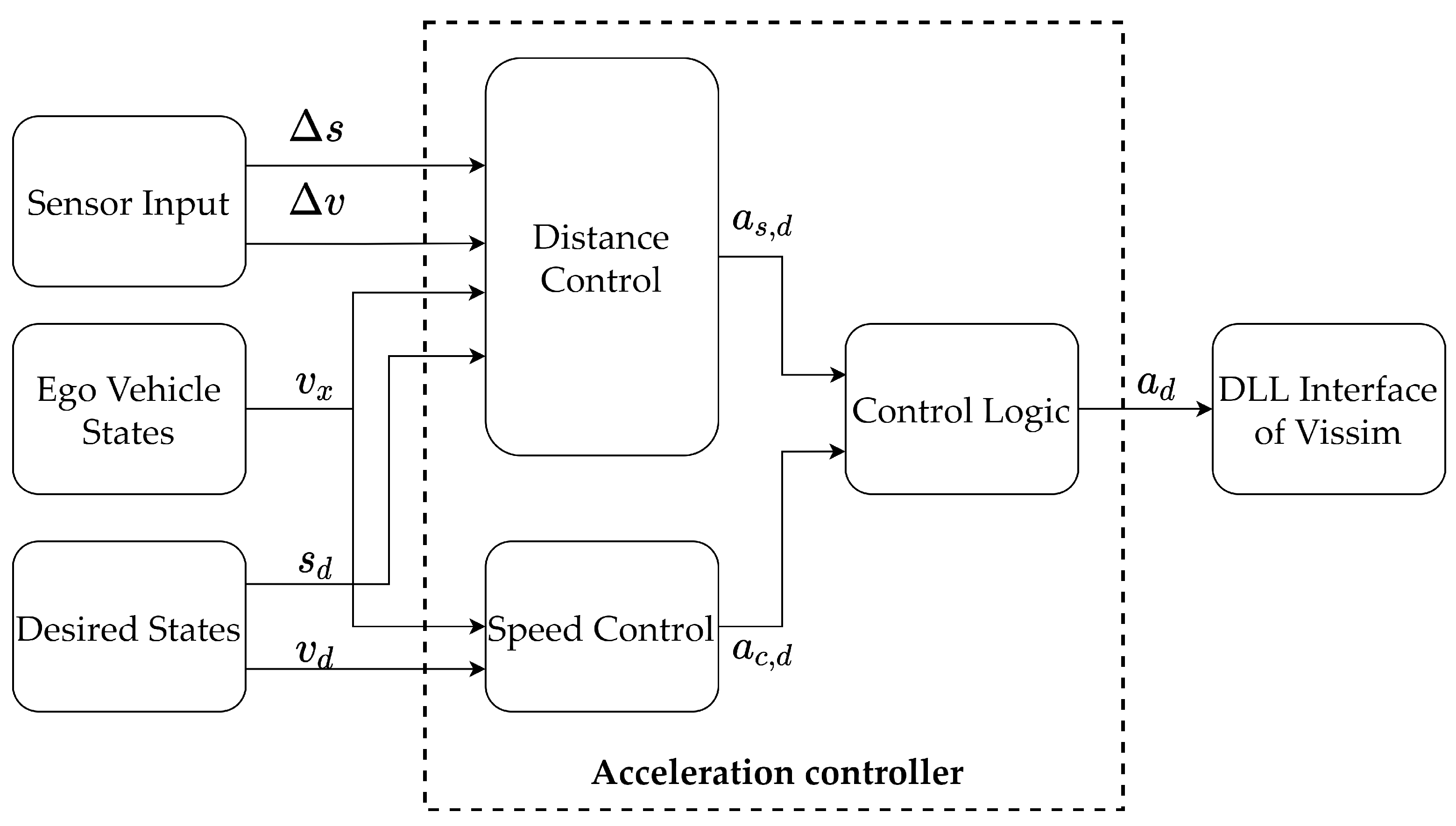
As one of the already serialized and common longitudinal controllers, the Adaptive Cruise Control (ACC) has the task to maintain a desired longitudinal speed or distance to a preceding vehicle. The norm International Organization for Standardization (ISO) 22179:2009 [23] defines the Full Speed Range Adaptive Cruise Control (FSRA), which allows control not only while free-flowing but also for congested traffic conditions. The system regulates the velocity of the ego vehicle depending on the vehicles in front and other traffic objects. Furthermore, if the FSRA-type system is used, the controller attempts to stop behind an already tracked vehicle within limited deceleration capabilities. The presented FSRA algorithm is developed based on a longitudinal vehicle model, the speed and distance controller introduced in [24]. The overall control scheme of the FSRA implementation process is depicted in Figure 4. The input signal is separated into three types, sensor inputs, ego vehicle states, and desired vehicle states. For the sensor input, they are relative speed and distance to a target vehicle provided, respectively, by the sensor model and transmitted to the distance control. As shown in Figure 1, the current traffic vehicle states can be read directly from Vissim. Therefore, the longitudinal ego vehicle velocity is transmitted to the distance controller and speed controller. For the desired states, the desired velocity and safe distance are predefined by the user. Additionally, an acceleration controller is used for developing longitudinal control algorithms, which means that the distance and speed controller generates the desired acceleration and , respectively. The control logic calculates a final desired acceleration, , which is forwarded to control a Vissim traffic vehicle through a DLL interface. All the values of model parameters are set according to [25], which depends on reasonable literature.
2.4.2. Lateral Control
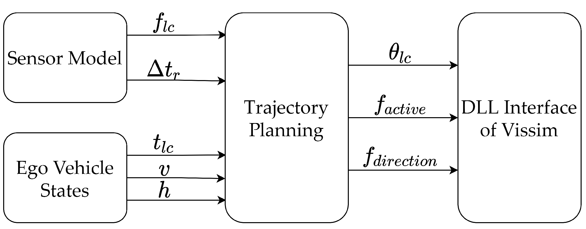
The lateral control of the HAV mainly simulates the lane change function for a vehicle. For an autonomous lane change on SAE level 3, there is still no ISO norm defined. However, the ISO 21202:2020 [26] norm deals with Partially Automated Lane Change Systems (PALS). It describes basic control strategies, basic driver interface elements, minimum requirements for reaction to failure, minimum functionality requirements, and performance test procedures for a PALS. However, this will only be possible on a road where no pedestrian or other non-motorized vehicle is taking part in the traffic. For autonomous lane change of HAV, it has to observe the position of the car within the lane as well as the adjacent lanes and obstacles in the vicinity. Meanwhile, the ego vehicle can initiate a lane change on its own, as defined by PEGASUS [13]. Figure 5 presents a complete lateral control logic. The sensor model determines lane change decision based on the target car in front of the ego car on the same lane and the surrounding driving situation in the adjacent lane. It thus sends a fused calculation of the TTC and lane change indication from sensor model to Trajectory Planning Block (TPB). Meanwhile, TPB receives the time consumed for the whole process of lane change , vehicle speed at the moment the lane change is triggered, and the lateral displacement h in real-time from Vissim. However, consider a corner case where an accelerating car may suddenly drive from behind during a lane change. In this case, TPB should abort the lane change action and re-plan back to the initial lane based on the rear TTC provided by the sensor model. In the end, TPB converts the inputs to the heading angle of the vehicle, lane change active command and lane change direction. These signals are transmitted to the DLL interface to control the Vissim traffic vehicles until lane change action is finished. Therefore, lane change trajectory and the back-planning trajectory generation in TPB are described as two important functions in the following:
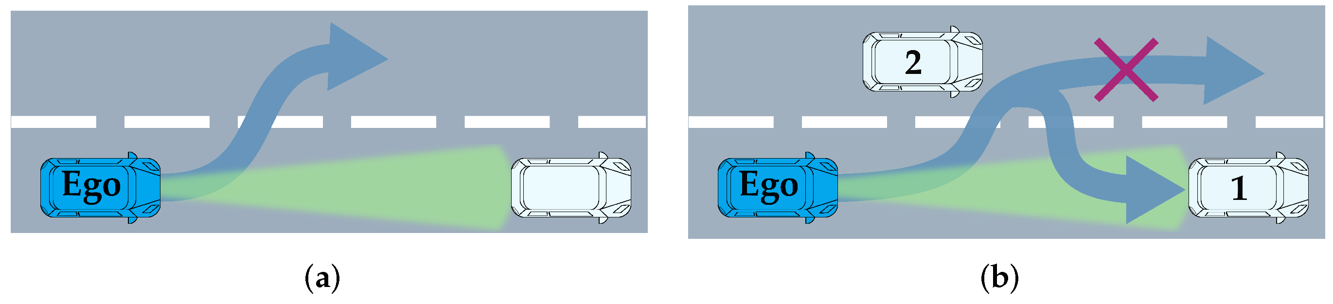
Regarding the lane change trajectory generation, the algorithm for the lane change behavior and the simulation implementation are presented in [27,28]. Based on these investigations, it is then known that the lane change is a time-based behavior. Therefore, the displacement of the vehicle from the center of the road can be derived in the trajectory equation for the lane change. The lateral and longitudinal trajectories are calculated by the polynomial Equations which are determined in Equations (4) and (5), respectively. With this method, a smooth trajectory is composed of only a few points. Meanwhile, the acceleration profile is calculated by Equation (6) in order to better and realistically match the lateral motion, where is maneuver time and calibrated to , which corresponds to an average time according to [27]. Referring to the description of the longitudinal behavior in [28], the maximum acceleration value can be set to = 1.2 m/s . For a complete lane change action = 3.5 m, which represents the displacement from one center line to the other (lane width). The entire process of lane change has an acceleration at the beginning phase and a gradual decrease in speed after the maneuver is completed. As shown in Figure 6a, the ego car detects a slower car ahead and that the adjacent lane is available for a lane change. Thus, a trajectory is generated.
In back-planning trajectory generation, is continuously checked as a safety standard until the lane change is completed. Lane change is aborted if the safety criterion fails to be met. Figure 6b presents a typical scenario. In this scenario, the ego car plans to change lane to pass the slower Car 1 in front of it, but a fast approaching Car 2 forces the ego car to abandon the lane change and move back to the initial lane. At this moment, h in Equation (4) is adjusted according to the lateral displacement between the current vehicle position and the initial point. Therefore, the lane change abortion path is generated by Equations (4)–(6). The HAV drives back to its original lane following the abortion path. With the lane change abortion mechanism, lane change safety of HAV can be guaranteed.
2.5. Connected and Automated Vehicle Model
Based on the HAV model introduced in the previous section, the CAV model is proposed to simulate a realistic environment with a V2V cooperative lane change function. Wireless technologies are rapidly evolving. This evolution provides opportunities to use these technologies in support of advanced vehicle safety applications and crash avoidance countermeasures [29]. Compared to the HAV model, CAV share their positions, speeds, accelerations, and states with each other, which has a greater impact on the upstream vehicles in the adjacent lane. Therefore, in this section, the CAV model focuses more on the cooperation and communication between vehicles. The preliminary application communication scenario requirements are defined in [30]. Lane change warning function should support a maximum distance of up to 150 m.
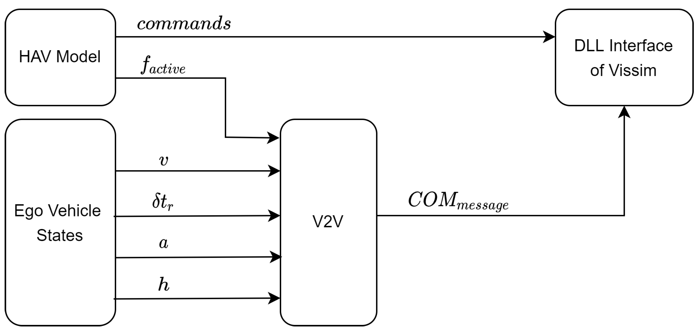
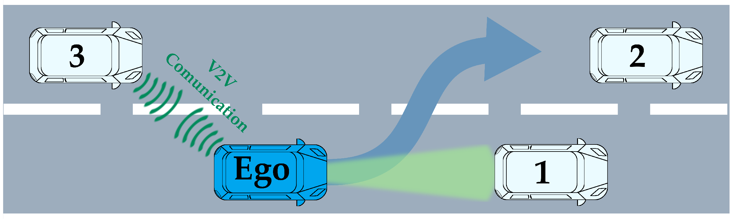
As the CAV has the basic functions of the HAV illustrated in Figure 7, it has the same lateral and longitudinal control mechanism and commands signals sent to DLL interface. Meanwhile, the V2V block receives state signals from HAV model and Vissim (i.e., current ego car speed v and acceleration a, rear TTC and lateral displacement h). Additionally, in order to simulate communication between vehicles, the ego car will broadcast an encapsulated lane change warning messages once lane change flag is triggered, with a radius of 150 m around the current ego car. Therefore, all CAV within the signal coverage area will receive this signal, and the relevant vehicle will be able to adjust its speed based on received encapsulated information. A typical scenario is shown in Figure 8; Car 3 is a CAV with V2V communication and follows Car 2. When the ego car detects Car 1 ahead, and the adjacent lane meets the lane change conditions, a lane change warning messages are broadcast before the lane change is triggered. After Car 3 receives the warning messages from the ego car, it will change the target car from Car 2 to ego car in longitudinal control. The ego car V2V broadcast communication messages to Car 3 in real-time during the lane change. Car 3 changes longitudinal movement according to V2V signals to reserve safe space for the ego car during the lane change.
3. Simulation
The emerging AV will definitely change the travel demand; however, whether this change is positive or negative is still under research. To simulate the current realistic traffic conditions, traffic flow was generated based on the data measured by KIRA (Transportation Information System Database of Hungary). Based on historical information provided by this database, the volume on the main road was set to 1440 vehicles/h, and the volume on the ramp was set to 312 vehicles/h, with eight percent of them Heavy Goods Vehicles (HGV). As mentioned above, the HAV and CAV will be introduced to the road system gradually. Based on this view, 31 scenarios representing different vehicle model combinations were simulated. Scenarios 1–11 contain CAV and Human Drive Vehicles (HDV), the penetration rates of CAV ranging from 0% to 100% with 10% step. HDV are represented by the calibrated Wiedemann 99 model in Vissim. Similarly, scenarios 12–21 contain the HAV model and HDV, the penetration rates of HAV ranging from 0% to 100% with 10% steps. Scenario 22–31 are a mix of three vehicle models with 20% steps. Each simulation involves a 1 h period, from 480 s to 4080 s with the first 480 s as warm-up time.
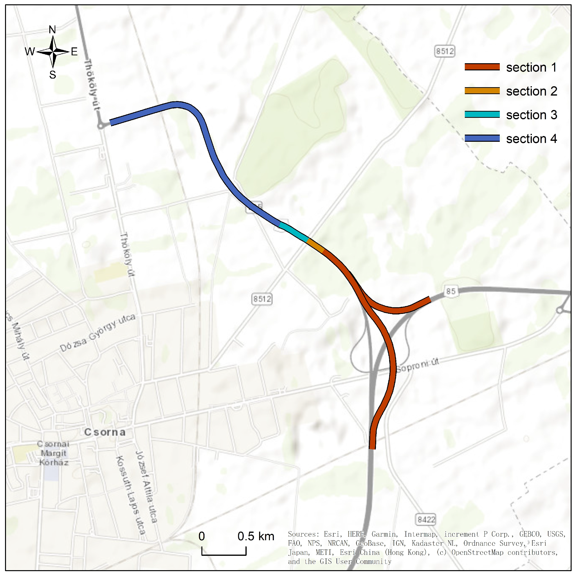
The test scenario is the upstream part of the M86 motorway. This road is close to the town of Csorna in northwestern Hungary (Győr-Moson-Sopron County, West Transdanubia region), connecting Szombathely with Győr, towards Budapest. The M86 is part of the TEN-T network [31] and also part of Hungarian State Public Road Network. Currently, the M86 is only in service between Szombathely and Csorna, with plans to extend north and south. This road is constructed to support the development and testing of autonomous vehicles. Figure 9 illustrates the overall 3.4 km profile of the M86 where the four sections of the road are marked:
- Section 1: two 3.50 m wide lanes are available for vehicles to travel. However, this section is connected to other roads. Thus, there is a ramp, which allows traffic from another motorway to merge into the main M86 road. Additionally, there are additional acceleration lanes connected to the ramp. Each vehicle can adjust vehicle speed in order to safely merge into the traffic. Therefore, this section of road has a great impact on the traffic speed in the simulation due to the complex traffic environment, which also proposes a challenge to the driving model.
- Section 2: This is a common two-lane section of approximately 300 m long, with two 3.50 m wide lanes. There will be some traffic merging into the main road from the acceleration lane coming out of the ramp extension.
- Section 3: At the end of the extended acceleration section, the dual carriageway will merge into a single carriageway, so there will be a lot of lane changes generated in this section.
- Section 4: The last section is a single lane with 3.5 m width up to the roundabout. This section of the road is relatively simple and has no lane changing behavior.
In order to make the simulation scenario reproduce the real road conditions and environment, a digital twin-based M86 motorway is generated, including every detail of test environments at high accuracy. Ref. [32] introduced high precision mapping to build an ultra-high definition map based on the road geometry. Meanwhile, the M86 road network has been used in [33] as virtual test scenarios, and its accuracy can reach ±2 cm, this accuracy is enough to ensure the effectiveness of the test and verification. As consequence, our simulation results are more realistic.
4. Result and Discussion
Through the presented comprehensive simulation system, the operation process of different proportions of autonomous vehicle models were simulated. The simulated data over the whole network are collected every 60 s interval. As the most indicative and intuitive parameters for the network status, the average speed of the network, the total travel time, and the average delay are used to evaluate traffic efficiency. The average speed is calculated by dividing total distance vehicles traveled by total travel time. The average delay is calculated by dividing total delay by the number of vehicles in the network plus the number of vehicles that have arrived. This delay is obtained by subtracting the actual distance traveled in the time step and desired speed from the duration of the time step.
Table 1 shows the simulation results of the mix of three vehicle models. The negative impact of the introduction of SAE level 3+ AV on traffic efficiency is evident observed from the simulated data. Compared to CAV, this negative effect is worse when HAV isintroduced to the network. This can be explained by an over perfect Wiedemann 99 model and as, compared to the human drivers that may take aggressive driving behavior, SAE level 3+ AV will not take any risky behavior when changing lane. Furthermore, SAE level 3+ AV require much larger gaps to perform a lane change than human drivers, which causes congestion at the merging area.
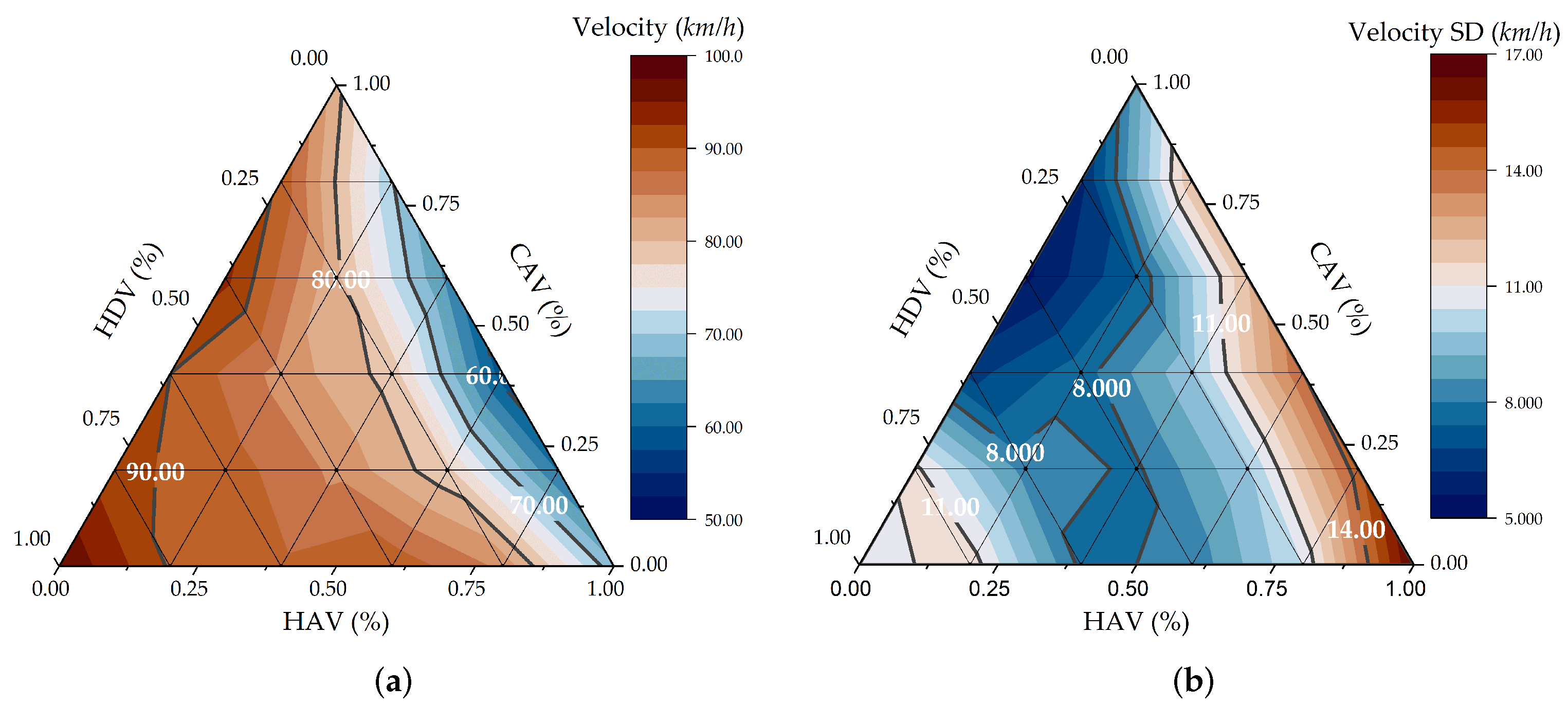
To intuitively present the relationship between the penetration rate of the three vehicle models and the average speed, Figure 10a was drawn in ternary plots. It graphically depicts the penetration rate of the three vehicle models from 0% to 100% as the three sides in an equilateral triangle. The color inside the triangle indicates the average speeds over the network. At every point within the triangle, the ratio of each combination is inversely proportional to the distance from the corner. Combining Table 1 and Figure 10a, it can be known that in the mixed flow, 40% CAV and 60% HDV show the best traffic efficiency, with the highest travel speed and the shortest travel time. Although the introduction of SAE level 3+ AV has a negative impact on total travel time and average speed, average delays in mixed traffic flow are significantly reduced. Especially in 100% CAV scenarios, the average delay dropped from 7.32 s to 0.51 s. The standard deviation plot of average speed in Figure 10b demonstrated the huge advantage of mixed flow consisting of CAV and HDV on the traffic stability. A smaller standard deviation means that the speed measurements are closer to the mean speed, which represents that the vehicles on the network can travel at a relatively uniform speed.
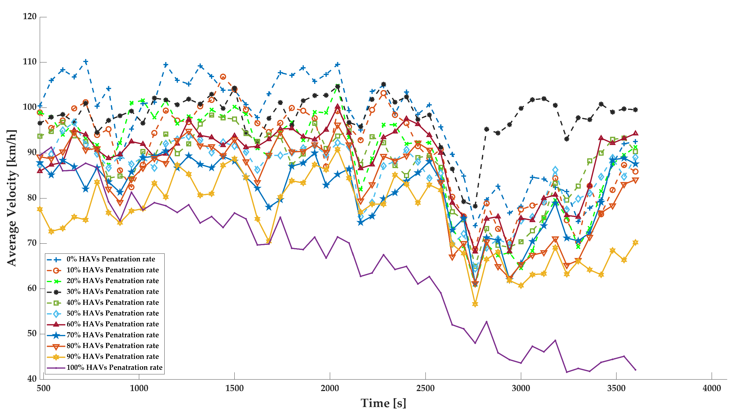
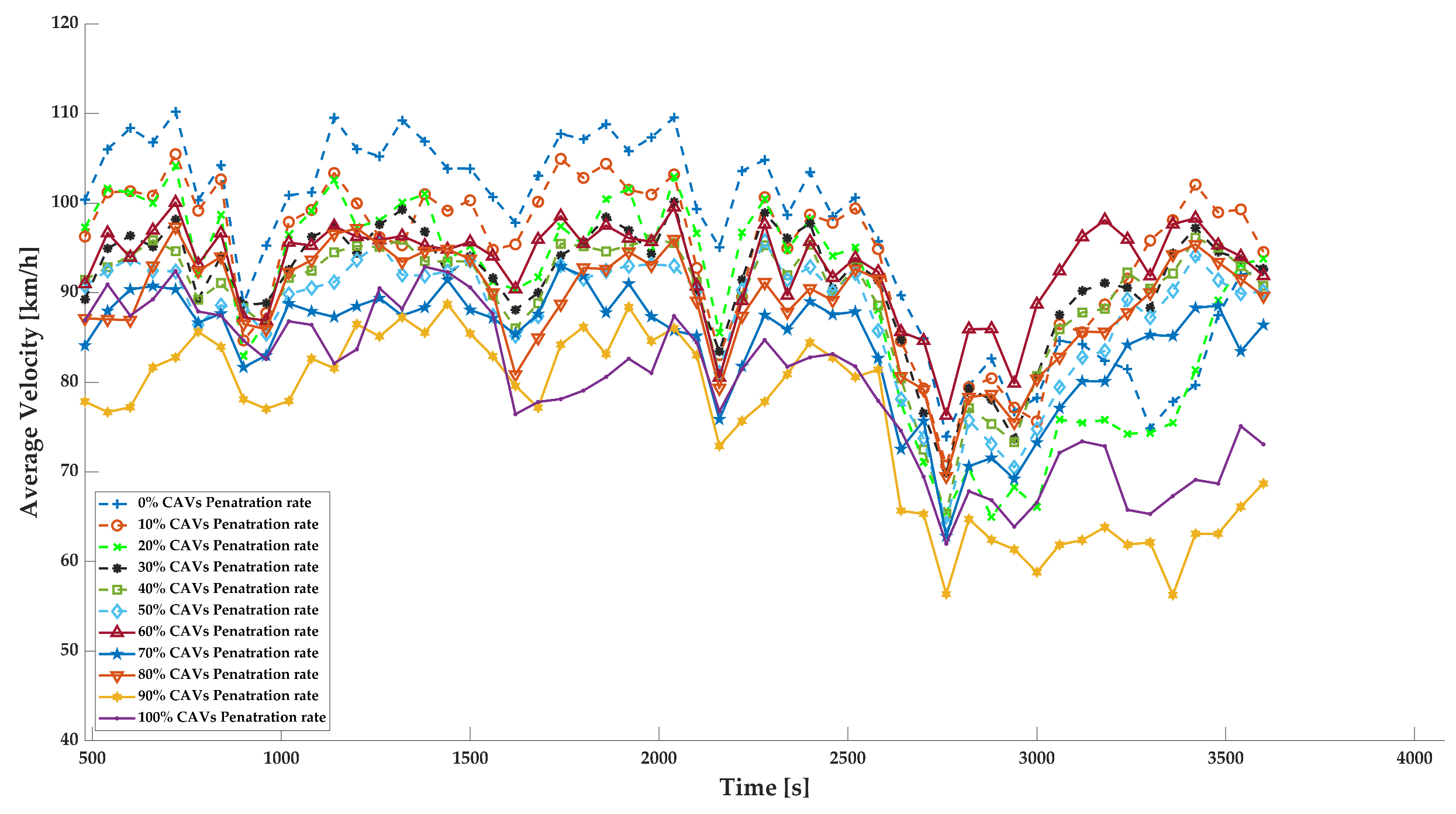
Figure 11 and Figure 12 present the changes of average speed with simulation time for various penetration rates of HAV and CAV, respectively. Overall, the introduction of HAV or CAV individually will cause the speed drop. For mixed traffic flow of HAV and HDV, 30% HAV with 70% HDV can generally keep the average speed at 100 km/h. Congestion can be observed at the end of simulation on the 100% HAV scenario; the average speed drops down to 40 km/h. It is foreseeable that, as the simulation time increases, the network will be fully blocked. This phenomenon can be explained by the much larger gap required by the HAV than human drivers when changing lanes. In addition, due to comfort considerations, the maximum acceleration of HAV is smaller than that of HDV, which results in the fact that when the network is full of HAV, the traffic downstream of the bottleneck decreases, and the upstream situation deteriorates.
Although the introduction of CAV individually also has a negative impact on the road network performance, due to the connection and cooperation functionality of CAV, the distribution of average speed is more concentrated than that of HAV. In the later stages of the simulation, as the penetration rate of CAV in the network increases, they can make full use of their connectivity to travel with small gaps, change lane faster, and absorb shock wave. Focusing on speed change, we see that under a high CAV penetration rate, the speed of the network shows a continuous growth tendency.
5. Conclusions
This paper demonstrates the potential effects of the introduction of HAV and CAV on a real-world network. A microscopic traffic simulation framework that integrates vehicle models with different automated driving functions was constructed. These functions were implemented as an external driver model in the microscopic traffic simulator PTV Vissim. The framework was tested in a detailed digital twin based on the M86 motorway located in the southwest of Hungary. A case study consisting of different scenarios was performed to declare the effects of various combinations of HDV, HAV, and CAV. The traffic demand was obtained from real traffic counts. The possible combinations in 10% and 20% steps of the variable penetration rates per vehicle model formed 31 simulations. Each simulation was performed within a 1 h time period. Simulation results indicate the introduction of HAV and CAV deteriorating network performance. HDV outperformed HAV and CAV because HDV may take aggressive driving behaviors and is able to function over the speed limit. This characteristic is magnified by the presence of the ramp in the network. Among multitude scenarios with mixed traffic flow, the combination of 60% CAV and 40% HDV possess the optimal traffic performance in terms of average speed, total travel time, and average delay.
Due to the connectivity between CAV, the uniformity of speed was better in scenarios with high CAV penetration rates, which led to the excellent driving stability and the inhibition of the formation of traffic oscillations. In addition, the high CAV penetration rates in the network result in a significant reduction in traffic delays.
Author Contributions
Conceptualization, X.F. and H.L.; methodology, H.L.; simulation, X.F.; validation, X.F. and H.L.; writing—original draft preparation, X.F. and H.L.; writing—review and editing, X.F., H.L., T.T. and A.E.; supervision, T.T. and A.E; project administration, T.T., A.E. and M.F. All authors have read and agreed to the published version of the manuscript.
Funding
The research was supported by the Hungarian Government and co-financed by the European Social Fund through the project “Talent management in autonomous vehicle control technologies” (EFOP-3.6.3-VEKOP-16-2017-00001).
Institutional Review Board Statement
Not applicable.
Informed Consent Statement
Not applicable.
Data Availability Statement
Not applicable.
Acknowledgments
The research was supported by the Hungarian Government and co-financed by the European Social Fund through the project “Talent management in autonomous vehicle control technologies” (EFOP-3.6.3-VEKOP-16-2017-00001).
Conflicts of Interest
The authors declare no conflict of interest.
References
- Sayer, J. Adaptive Cruise Control (ACC) Operating Characteristics and User Interface: Standard J2399; Society of Automotive Engineers: Warrendale, PA, USA, 2003. [Google Scholar]
- Wróblewski, P.; Drożdż, W.; Lewicki, W.; Miązek, P. Methodology for assessing the impact of aperiodic phenomena on the energy balance of propulsion engines in vehicle electromobility systems for given areas. Energies 2021, 14, 2314. [Google Scholar] [CrossRef]
- Wróblewski, P.; Kupiec, J.; Drożdż, W.; Lewicki, W.; Jaworski, J. The economic aspect of using different plug-in hybrid driving techniques in urban conditions. Energies 2021, 14, 3543. [Google Scholar] [CrossRef]
- Norm. SAE J3016_2016; Taxonomy and Definitions for Terms Related to Driving Automation Systems for On-Road Motor Vehicles. SAE International: Warrendale, PA, USA, 2016.
- Catapult Connected Places. Market Forecast for Connected and Autonomous Vehicles; Technical Report; Department for Transport and Centre for Connected and Autonomous Vehicles, Smart Transport: Peterborough, UK, 2021. [Google Scholar]
- Fang, X.; Tettamanti, T. Change in Microscopic Traffic Simulation Practice with Respect to the Emerging Automated Driving Technology. Period. Polytech. Civ. Eng. 2022, 66, 86–95. [Google Scholar] [CrossRef]
- Goodall, N.J.; Lan, C.L. Car-following characteristics of adaptive cruise control from empirical data. J. Transp. Eng. Part A Syst. 2020, 146, 04020097. [Google Scholar] [CrossRef]
- Leyn, U.; Vortisch, P. Calibrating VISSIM for the German highway capacity manual. Transp. Res. Rec. 2015, 2483, 74–79. [Google Scholar] [CrossRef]
- Lu, Z.; Fu, T.; Fu, L.; Shiravi, S.; Jiang, C. A video-based approach to calibrating car-following parameters in VISSIM for urban traffic. Int. J. Transp. Sci. Technol. 2016, 5, 1–9. [Google Scholar] [CrossRef] [Green Version]
- Li, Q.; Li, X.; Huang, Z.; Halkias, J.; McHale, G.; James, R. Simulation of Mixed Traffic with Cooperative Lane Changes. Comput Aided Civ Inf. 2021. [CrossRef]
- Milanés, V.; Shladover, S.E. Modeling cooperative and autonomous adaptive cruise control dynamic responses using experimental data. Transp. Res. Part C Emerg. Technol. 2014, 48, 285–300. [Google Scholar] [CrossRef] [Green Version]
- Papadoulis, A.; Quddus, M.; Imprialou, M. Evaluating the safety impact of connected and autonomous vehicles on motorways. Accid. Anal. Prev. 2019, 124, 12–22. [Google Scholar] [CrossRef] [PubMed] [Green Version]
- The Highway-Chauffeur. Requirements and Conditions—Booth No. 04. Pegasus. In Proceedings of the PEGASUS Symposium 2019, Glasgow, UK, 10–12 April 2019; PEGASUS: Braunschweig, Germany, 2019. [Google Scholar]
- Fellendorf, M. VISSIM: A microscopic simulation tool to evaluate actuated signal control including bus priority. In Proceedings of the 64th Institute of Transportation Engineers Annual Meeting, Dallas, TX, USA, 16–19 October 1994; Springer: Berlin/Heidelberg, Germany, 1994; Volume 32, pp. 1–9. [Google Scholar]
- Behrisch, M.; Bieker, L.; Erdmann, J.; Krajzewicz, D. SUMO—Simulation of urban mobility: An overview. In Proceedings of the SIMUL 2011, the Third International Conference on Advances in System Simulation, ThinkMind, Barcelona, Spain, 23–29 October 2011. [Google Scholar]
- Halati, A.; Lieu, H.; Walker, S. CORSIM-corridor traffic simulation model. In Proceedings of the Traffic Congestion and Traffic Safety in the 21st Century: Challenges, Innovations, and Opportunities Urban Transportation Division, ASCE; Highway Division, ASCE; Federal Highway Administration, USDOT; and National Highway Traffic Safety Administration, USDOT, Chicago, IL, USA, 8–11 June 1997. [Google Scholar]
- Cameron, G.D.; Duncan, G.I. PARAMICS—Parallel microscopic simulation of road traffic. J. Supercomput. 1996, 10, 25–53. [Google Scholar] [CrossRef]
- Tettamanti, T.; Varga, I. Development of road traffic control by using integrated VISSIM-MATLAB simulation environment. Period. Polytech. Civ. Eng. 2012, 56, 43–49. [Google Scholar] [CrossRef] [Green Version]
- Fellendorf, M.; Vortisch, P. Microscopic Traffic Flow Simulator VISSIM. In Fundamentals of Traffic Simulation; Springer: Berlin/Heidelberg, Germany, 2010; pp. 63–93. [Google Scholar]
- Szoke, L.; Aradi, S.; Becsi, T.; Gaspar, P. Vehicle Control in Highway Traffic by Using Reinforcement Learning and Microscopic Traffic Simulation. In Proceedings of the 2020 IEEE 18th International Symposium on Intelligent Systems and Informatics (SISY), Subotica, Serbia, 17–19 September 2020; IEEE: Piscataway, NJ, USA, 2020; pp. 21–26. [Google Scholar]
- Kawasaki, T.; Caveney, D.; Katoh, M.; Akaho, D.; Takashiro, Y.; Tomiita, K. Teammate Advanced Drive System Using Automated Driving Technology; Technical Report; SAE International: Warrendale, PA, USA, 2021. [Google Scholar]
- Schneider, M. Automotive radar-status and trends. In Proceedings of the German Microwave Conference, Ulm, Germany, 5–7 April 2005; pp. 144–147. [Google Scholar]
- ISO 22179:2009; Intelligent Transport Systems—Full Speed Range Adaptive Cruise Control (FSRA) Systems–Performance Requirements and Test Procedures. Norm, International Organization for Standardization: Geneva, Switzerland, September 2009.
- Bernsteiner, S. Integration of Advanced Driver Assistance Systems on Full-Vehicle Level-Parametrization of an Adaptive Cruise Control System Based on Test Drives; Technical University Graz: Graz, Austria, 2016. [Google Scholar]
- Li, Y.; Wang, H.; Wang, W.; Xing, L.; Liu, S.; Wei, X. Evaluation of the impacts of cooperative adaptive cruise control on reducing rear-end collision risks on freeways. Accid. Anal. Prev. 2017, 98, 87–95. [Google Scholar] [CrossRef] [PubMed]
- ISO 21202:2020; Intelligent Transport Systems—Partially Automated Lane Change Systems (PALS)—Functional/Operational Requirements and Test Procedures. Norm, International Organization for Standardization: Geneva, Switzerland, April 2020.
- Samiee, S.; Azadi, S.; Kazemi, R.; Eichberger, A. Towards a decision-making algorithm for automatic lane change manoeuvre considering traffic dynamics. PROMET-Traffic Transp. 2016, 28, 91–103. [Google Scholar] [CrossRef] [Green Version]
- Nalic, D.; Li, H.; Eichberger, A.; Wellershaus, C.; Pandurevic, A.; Rogic, B. Stress Testing Method for Scenario-Based Testing of Automated Driving Systems. IEEE Access 2020, 8, 224974–224984. [Google Scholar] [CrossRef]
- Ždánsky, P.; Balák, J.; Rástočnỳ, K. Safety Integrity Evaluation of Safety Function. In Proceedings of the 2018 International Conference on Applied Electronics (AE), Pilsen, Czech Republic, 11–12 September 2018; IEEE: Piscataway, NJ, USA, 2018; pp. 1–6. [Google Scholar]
- Shulman, M.; Deering, R. Vehicle safety communications in the United States. In Proceedings of the Conference on Experimental Safety Vehicles, Wahshington, DC, USA, 18–21 June 2007. [Google Scholar]
- Gutiérrez, J.; Condeço-Melhorado, A.; López, E.; Monzón, A. Evaluating the European added value of TEN-T projects: A methodological proposal based on spatial spillovers, accessibility and GIS. J. Transp. Geogr. 2011, 19, 840–850. [Google Scholar] [CrossRef]
- Tihanyi, V.; Tettamanti, T.; Csonthó, M.; Eichberger, A.; Ficzere, D.; Gangel, K.; Hörmann, L.B.; Klaffenböck, M.A.; Knauder, C.; Luley, P.; et al. Motorway measurement campaign to support R&D activities in the field of automated driving technologies. Sensors 2021, 21, 2169. [Google Scholar] [CrossRef]
- Li, H.; Makkapati, V.P.; Nalic, D.; Eichberger, A.; Fang, X. A Real-time Co-Simulation Framework for Virtual Test and Validation on a High Dynamic Vehicle Test Bed. In Proceedings of the 32nd IEEE Intelligent Vehicle Symposium, Nagoya, Japan, 11–15 July 2021; IEEE Press: Piscataway, NJ, USA, 2021. [Google Scholar]
Figure 1.
Overview of the DLL driving model.

Figure 2.
TTC outcome possibility.

Figure 3.
Process of decision making based on TTC calculation.

Figure 4.
Longitudinal control schema in the driving model.

Figure 5.
Lateral control schema in the driving model.

Figure 6.
Lane change trajectory generation (a) a complete lane change trajectory planning; (b) an abortion trajectory generation.
Figure 6.
Lane change trajectory generation (a) a complete lane change trajectory planning; (b) an abortion trajectory generation.

Figure 7.
CAV model in the driving model.

Figure 8.
Cooperative lane change for CAV.

Figure 9.
The upstream network of the M86 motorway.

Figure 10.
(a) Average speed over the network with mixed traffic; (b) Standard deviation of average speed over the network with mixed traffic.
Figure 10.
(a) Average speed over the network with mixed traffic; (b) Standard deviation of average speed over the network with mixed traffic.

Figure 11.
Average speed over the network for the various HAV penetration rates.

Figure 12.
Average speed over the network for the various CAV penetration rates.


Table 1.
Traffic performance evaluation of the simulated network.
| Vehicle Composition | Average Speed over the Network (km/h) | Total Travel Time (s) | Average Delay (s) | ||
|---|---|---|---|---|---|
| HAV | CAV | HDV | |||
| 0% | 0% | 100% | 97.33 | 3462.04 | 7.32 |
| 0% | 20% | 80% | 90.69 | 3721.97 | 7.33 |
| 0% | 40% | 60% | 90.00 | 3699.27 | 5.36 |
| 0% | 60% | 40% | 93.20 | 3577.72 | 3.38 |
| 0% | 80% | 20% | 89.25 | 3738.47 | 2.13 |
| 0% | 100% | 0% | 81.02 | 4133.17 | 0.51 |
| 20% | 0% | 80% | 89.70 | 3776.68 | 7.12 |
| 40% | 0% | 60% | 87.98 | 3793.02 | 5.18 |
| 60% | 0% | 40% | 89.35 | 3756.64 | 3.46 |
| 80% | 0% | 20% | 84.44 | 3997.94 | 2.21 |
| 100% | 0% | 0% | 68.13 | 5085.81 | 1.03 |
| 20% | 20% | 60% | 88.82 | 3774.40 | 5.32 |
| 20% | 40% | 40% | 84.07 | 3967.40 | 4.43 |
| 20% | 60% | 20% | 80.65 | 4125.98 | 2.70 |
| 20% | 80% | 0% | 70.21 | 4125.98 | 0.78 |
| 40% | 20% | 40% | 84.41 | 3941.23 | 4.03 |
| 40% | 40% | 20% | 78.98 | 4223.81 | 2.87 |
| 40% | 60% | 0% | 64.31 | 5221.23 | 1.04 |
| 60% | 20% | 20% | 78.19 | 4253.08 | 2.62 |
| 60% | 40% | 0% | 58.58 | 5834.29 | 1.35 |
| 80% | 20% | 0% | 62.22 | 5496.21 | 1.08 |
Publisher’s Note: MDPI stays neutral with regard to jurisdictional claims in published maps and institutional affiliations. |
© 2022 by the authors. Licensee MDPI, Basel, Switzerland. This article is an open access article distributed under the terms and conditions of the Creative Commons Attribution (CC BY) license (https://creativecommons.org/licenses/by/4.0/).
Share and Cite
MDPI and ACS Style
Fang, X.; Li, H.; Tettamanti, T.; Eichberger, A.; Fellendorf, M. Effects of Automated Vehicle Models at the Mixed Traffic Situation on a Motorway Scenario. Energies 2022, 15, 2008. https://doi.org/10.3390/en15062008
AMA Style
Fang X, Li H, Tettamanti T, Eichberger A, Fellendorf M. Effects of Automated Vehicle Models at the Mixed Traffic Situation on a Motorway Scenario. Energies. 2022; 15(6):2008. https://doi.org/10.3390/en15062008
Chicago/Turabian StyleFang, Xuan, Hexuan Li, Tamás Tettamanti, Arno Eichberger, and Martin Fellendorf. 2022. "Effects of Automated Vehicle Models at the Mixed Traffic Situation on a Motorway Scenario" Energies 15, no. 6: 2008. https://doi.org/10.3390/en15062008
Note that from the first issue of 2016, this journal uses article numbers instead of page numbers. See further details here.