Robust Sliding Mode Fuzzy Control of Industrial Robots Using an Extended Kalman Filter Inverse Kinematic Solver

Abstract

This paper presents a sliding mode fuzzy control approach for industrial robots at their static and near static speed (linear velocities less than 5 cm/s). The extended Kalman filter with its covariance resetting is used to translate the coordinates from Cartesian to joint angle space. The translated joint angles are then used as a reference signal to control the industrial robot dynamics using a sliding mode fuzzy controller. The stability and robustness of the proposed controller is proven using an appropriate Lyapunov function in the presence of parameter uncertainty and unknown dynamic friction. The proposed controller is simulated on a 6-DOF industrial robot, namely the Universal Robot-UR5, considering the maximum allowable joint torques. It is observed that the proposed controller can successfully control UR5 under uncertainties in terms of unknown dynamic friction and parameter uncertainties. The tracking performance of the proposed controller is compared with that of the sliding mode control approach. The simulation results demonstrate superior performance of the proposed approach over the sliding mode control method in the presence of uncertainties.

1. Introduction

Industry 4.0 is the fourth generation of industry. It has accommodated advanced machine learning approaches as well as artificial intelligence into the core of manufacturing to improve production [1,2]. This has resulted in more intelligent factory floors that can respond to customer needs through increasingly customizable products [3,4]. Robots serve as an indispensable part of industrial environments, increasing productivity and reducing design-to-market time through their ability to efficiently improve production in highly repetitive tasks [5]. Precision of the factory elements is a primary issue that must be improved to increase manufacturing performance [6,7]. Industrial tasks on a factory floor, such as object handling [8] and manipulation [9], require ahigh level of precision while maintaining safe operation. Industrial robots are serial architectures, with several joints making up their construction. Their architecture results in high coupling between different link dynamics. Modelling uncertainties include simplifications, dead zones, backlashes [5], and variable load for industrial robots. In particular, operating at or near static conditions can cause dynamic control problems due to changes in motion state. We believe that a sliding mode control approach is a robust control method that can be used to guarantee the tracking behavior of industrial robots in finite time in the presence of matched uncertainties [10].

The sliding mode control approach is a nonlinear and robust control approach. In this controller, the desired behavior of the robot is defined in terms of a sliding surface [11,12]. The Lyapunov stability theorem is used to design the control signal to guarantee reaching the sliding surface [13,14,15,16]. When the states of the robot reach the sliding surface, the high frequency switching law maintains sliding mode for a stable reference signal [13,14]. The most prominent features of sliding mode control for industrial robots are robustness to unmodelled dynamic and unknown variable loads [17].

To track a desired Cartesian space coordinate, an inverse kinematic solver is required to translate industrial robot motion in a Cartesian space to its desired joint space motion. There exist different approaches to solve the inverse kinematic of industrial robots. Geometric approaches are used to find the inverse kinematic of the robot in a closed form [18]. Geometrical approaches to solve inverse kinematic have already been used for planar hyper-redundant manipulators [18,19], the 7R 6-DOF Robot-Manipulator [20], and hybrid parallel-serial five-axis machine tools [21]. Neural networks [22,23,24], neuro-fuzzy approaches [25], and deep neural networks [26,27] can be put in the second category of inverse kinematic solvers. The third category is the one that uses estimation algorithms to solve the inverse kinematic. Although the kinematic model of industrial robots is highly nonlinear, it can be linearized using Taylor expansions. Estimation algorithms such as Levenberg–Marquardt [28], least squares [29,30], recursive least square, and extended Kalman filter [30,31] may also be utilized to find the corresponding joint angles of robots. The second and third categories of inverse kinematic solvers can be identified as machine learning approaches. Among the listed estimation algorithms, the extended Kalman filter is used in [32,33] for the accurate inverse kinematic and calibration of industrial robots. This method has previously outperformed least squares for solving the inverse kinematic problem of the Kawasaki RS10N industrial robot and a 4-DOF laboratory setup in terms of accuracy as well as number of iterations [32,33].

Fuzzy systems are effective approaches to deal with uncertainty in control systems. They can effectively approximate any smooth nonlinear function, provided enough rules are used in their structure. Fuzzy systems have been used to enhance the performance of classical control approaches such as the model reference control method and sliding mode controllers [34]. The combination of fuzzy systems and sliding mode approaches results in a robust adaptive control approach, which benefits from the rigorous mathematical backbone of sliding mode control theory and the adaptation capabilities of fuzzy systems. Such approaches have been used to control induction servomotors, anti-lock braking systems [35,36], and active suspension systems for vehicles [37,38].

In this paper, a sliding mode fuzzy control (SMFC) approach is used to control an industrial robot in its low-speed motion (linear velocity less than 5 cm/s). The reference signal is given in terms of Cartesian position and orientation, which is then translated to the joint space using the inverse kinematic approach. The inverse kinematic approach used in this paper uses an extended Kalman filter for joint angle estimation. This approach has been shown to find the desired robot joint angles in a smaller number of iterations compared to the least square method [32]. In this paper, the sample time considered for the inverse kinematic solver and the controller are both equal to $1\mathrm{msec}$. Different from the sliding mode controller, which was designed for UR5 in [39], the control signal designed in this paper does not include angular acceleration, which makes it easier to implement. The desired behavior of the industrial robot is defined in terms of a sliding mode, and the parameter update rules for the fuzzy system in the SMFC are derived from Lyapunov stability theorem. The robustness of the controller in the presence of unknown friction torques and parameter uncertainty is analyzed using the Lyapunov function. Simulations are performed under MATLAB/Simulink^® software. The Cartesian space reference signal is given with slow changes to ensure results are tracked at near static speeds (up to 5 cm/s). The results demonstrate the implementability, showing the satisfactory performance of the overall controller in the presence of unknown friction and parameter uncertainties in the robot dynamics. Comparison is made to a previous sliding mode control approach, used to control UR5 [39]. The comparison results show a smaller tracking error value as compared to the sliding mode control approach used in [39] to control UR5. In summary, the contributions of the proposed approach over approaches in the literature are

• Use of an extended Kalman filter as an inverse kinematic solver along with SMFC to control industrial robots;
• Elimination of the necessity to include a second order time derivative of joint angles in the control law;
• Superior performance over the sliding mode controller for UR5 as presented in [39].

This rest of this paper is organized as follows. The dynamic model of the industrial robot and its kinematics are given in Section 2. The overall control architecture is proposed in Section 3, where the overall control architecture, adaptation laws, and the stability analysis of the system are discussed. The simulation results are given in Section 4, and concluding remarks are presented in Section 5.

2. Industrial Robot Dynamic and Kinematics

2.1. Industrial Robot Dyanmics

The general dynamic of a rigid link 6-DOF industrial robot can be formulated in terms of ordinary differential equations composed of interacting forces on the robot, as follows [40,41]:

$$M\left(q\right)\ddot{q}+C\left(q,\dot{q}\right)\dot{q}+G\left(q\right)+F\left(\dot{q}\right)=\tau ,$$

(1)

where $q\in {ℝ}^{6\times 1}$ is the robot joint angle vector, $M\left(q\right)\in {ℝ}^{6\times 6}$ represents the inertial forces in the industrial robot, $C\left(q,\dot{q}\right)\in {ℝ}^{6\times 6}$ represents the Coriolis and centrifugal forces, $G\left(q\right)\in {ℝ}^{6\times 1}$ presents the robot gravitational force terms, $F\left(\dot{q}\right)\in {ℝ}^{6\times 1}$ represents the dynamic friction terms of the robot, and $\tau \in {ℝ}^{6\times 1}$ presents the input torque vector to control the robot. The matrix $M\left(q\right)$ satisfies the following equation for the kinetic energy of the robot.

$$K=\frac{1}{2}{\dot{q}}^{T}M\left(q\right)\dot{q}$$

(2)

The elements of the vector $G\left(q\right)$, the gravitational forces of the robot, are partial derivatives of potential energy with respect to the corresponding robot joint angles.

$$g_k=\frac{\partial P}{\partial q_k},k=1,\dots ,6$$

(3)

where $P$ is the potential energy of the robot and $g_k$ represents the elements of the $G\left(q\right)$ vector such that $G\left(q\right)={\left[\begin{array}{ccc}{g}_1& \dots & g_6\end{array}\right]}^T.$ Furthermore, the elements of the matrix $C\left(q,\dot{q}\right)$, the Coriolis and centrifugal force matrix, satisfy the following equation:

$$c_{kj}={\displaystyle \sum }_{i=1}^n{c}_{ijk}\left(q\right){\dot{q}}_i$$

(4)

where $c_{ijk}\left(q\right)$ represents the Christoffel symbols [41]:

$$c_{ijk}\left(q\right)=\frac{1}{2}\left\{\frac{\partial d_{kj}}{\partial q_i}+\frac{\partial d_{ki}}{\partial q_j}-\frac{\partial d_{ij}}{\partial q_k}\right\}$$

(5)

Finally, $F\left(\dot{q}\right)$ represents the dynamic friction terms of the robot [42].

2.2. Inverse Kinematic Calculation for Industrial Robots

The forward kinematic is a function that finds the Cartesian coordinates of robot within 3D space as a function of its joint angles. The inverse kinematic is the reverse procedure to assign appropriate joint angles to industrial robots to maintain the desired position and orientation. There exist different solutions for the inverse kinematic for industrial robots at a given pose/alignment of the end-effector and many solutions to determine optimal results. Among them, an algorithm was recently investigated in [32] that uses an extended Kalman filter approach to estimate the joint angles of industrial robot. This approach contributes to a higher degree of precision as compared to least squares approaches to estimate the joint angles of industrial robots. Because of the high precision of this algorithm, we selected it for use in this paper. The link transformation matrix from the link $i$−1 to the link $i$ using the Denavit–Hartenberg (D–H) parameters of the robot depends on joint angles, as follows [43]:

$$\begin{array}{c}{}_1{}^{0}T=\left[\begin{array}{cccc}cos{\theta }_1& 0& sin{\theta }_1& 0\\ sin{\theta }_1& 0& -cos{\theta }_1& 0\\ 0& 0& 0& 0.08916\\ 0& 0& 0& 1\end{array}\right],{}_2{}^{1}T=\left[\begin{array}{cccc}cos{\theta }_2& -sin{\theta }_2& 0& -0.425cos{\theta }_2\\ sin{\theta }_2& cos{\theta }_2& 0& -0.425sin{\theta }_2\\ 0& 0& 0& 0\\ 0& 0& 0& 1\end{array}\right]\\ {}_3{}^{2}T=\left[\begin{array}{cccc}cos{\theta }_3& -sin{\theta }_3& 0& -0.392cos{\theta }_3\\ sin{\theta }_3& cos{\theta }_3& 0& -0.392sin{\theta }_3\\ 0& 0& 0& 0\\ 0& 0& 0& 1\end{array}\right],{}_4{}^{3}T=\left[\begin{array}{cccc}cos{\theta }_4& 0& sin{\theta }_4& 0\\ sin{\theta }_4& 0& -cos{\theta }_4& 0\\ 0& 1& 0& 0.1092\\ 0& 0& 0& 1\end{array}\right]\\ {}_5{}^{4}T=\left[\begin{array}{cccc}cos{\theta }_5& 0& -sin{\theta }_5& 0\\ sin{\theta }_5& 0& cos{\theta }_5& 0\\ 0& -1& 0& 0.0947\\ 0& 0& 0& 1\end{array}\right],{}_6{}^{5}T=\left[\begin{array}{cccc}cos{\theta }_6& -sin{\theta }_6& 0& 0\\ sin{\theta }_6& cos{\theta }_6& 0& 0\\ 0& 0& 1& 0.0823\\ 0& 0& 0& 1\end{array}\right]\end{array}$$

(6)

The industrial robot end effector position and orientation in the fixed world coordinate attached to the base of the industrial robot is calculated as the multiplication of all link transformation matrices.

$$T_e={}_6{}^{0}T={}_1{}^{0}T{}_2{}^{1}T{}_3{}^{2}T{}_4{}^{3}T{}_5{}^{4}T{}_6{}^{5}T$$

(7)

The overall end-effector position and orientation error can be approximated by linear superpositions of the joint angle deviations weighted by their sensitivity function.

$$\Delta T_e=\frac{\partial T_e}{\partial {\theta }_1}\Delta {\theta }_1+\dots +\frac{\partial T_e}{\partial {\theta }_6}\Delta {\theta }_6+H.O.T.$$

(8)

The parameter $\frac{\partial T_e}{\partial {\theta }_i}$ is the sensitivity function of the end-effector transformation matrix with respect to i-th joint angle of the robot and can be calculated analytically.

Remark 1. 

It is noted that in the industrial robot investigated in this paper, the only changeable D–H parameter is the joint angles of the robot ${\theta }_i$’s. However, in a more general case where other D–H parameters of the robot are changeable, the matrix $\Delta T_e$ is approximated as a linear superposition of all deviations in all D–H parameters, weighted by their corresponding sensitivity matrix.

According to [32], the extended Kalman filter estimation method results in a more precise positioning of the robot than the least squares solution. The EKF estimation iteratively estimates the joint angles of the robot as follows [36]:

$${\theta }^{k+1}={\theta }^k+K^k\left[T^d-h^k\left({\theta }^k\right)\right]$$

$$P^k=P^k{H}^k{\left(R+H^{kT}{P}^k{H}^k\right)}^{-1}$$

$$P^{k+1}=P^k-P^k{H}^{kT}{P}^k+Q^k$$

(9)

where ${\theta }^k={\left[\begin{array}{ccc}{\theta }_1^k& \dots & {\theta }_6^k\end{array}\right]}^T$ is the vector of the unknown joint angles of the robot at the k-th iteration, $P^k\in {ℝ}^{6\times 6}$ is the parameter covariance matrix at the k-th iteration, $R\in {ℝ}^{12}$ is the measurement noise covariance matrix, and $Q^k\in {ℝ}^{6\times 6}$ is the process noise covariance matrix. $H^k$ is defined as follows:

$$H^k={\left[\begin{array}{ccc}\frac{\partial h}{\partial {\theta }_1^k}& \dots & \frac{\partial h}{\partial {\theta }_6^k}\end{array}\right]}^T$$

(10)

and the function $h$ is a vector function of ${\theta }^k$, defined as follows:

$$h^k={\left[\begin{array}{ccc}\begin{array}{ccc}{T}_{e11}^k& \dots & T_{e14}^k\end{array}& \dots & \begin{array}{ccc}{T}_{e31}^k& \dots & T_{e34}^k\end{array}\end{array}\right]}^T$$

(11)

where $T_e$ is obtained from Equation (7). The function $T^d$ is the desired position and orientation of the robot in a vector form, as follows:

$$T_d={\left[\begin{array}{ccc}\begin{array}{ccc}{T}_{de11}& \dots & T_{de14}\end{array}& \dots & \begin{array}{ccc}{T}_{de31}& \dots & T_{de34}\end{array}\end{array}\right]}^T$$

(12)

where $T_{de}$ includes the desired position and orientation of the robot.

3. Control Architecture

3.1. Overall Control Structure

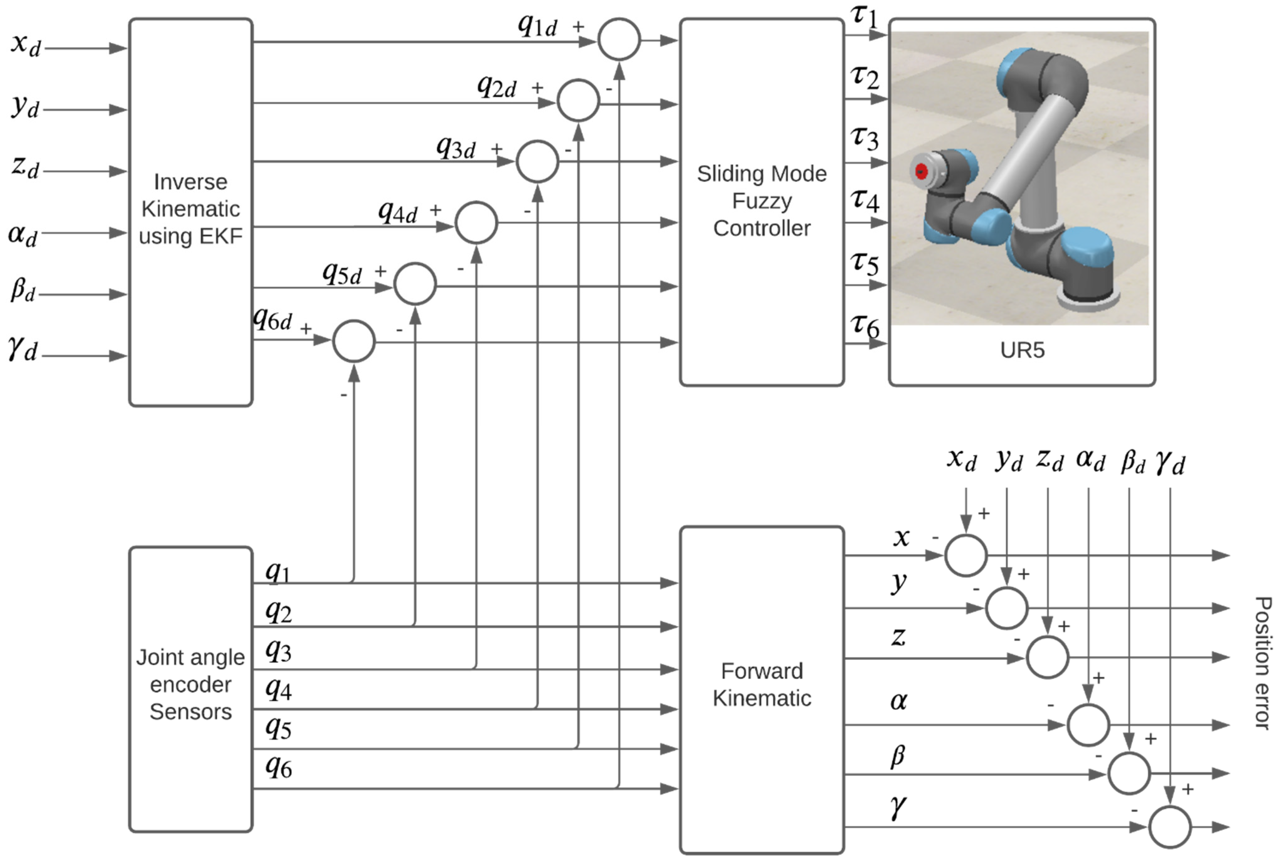
The overall control structure is denoted in Figure 1. The desired position of the robot end effector is denoted by ${\left[\begin{array}{ccc}{x}_d& y_d& z_d\end{array}\right]}^T$, and its desired orientation is represented by ${\left[\begin{array}{ccc}{\alpha }_d& {\beta }_d& {\gamma }_d\end{array}\right]}^T$. Using the inverse kinematic of the robot as explained in Section 2.2, it is possible to find the desired joint angles of the robot ${\left[\begin{array}{ccc}{q}_{1d}& \dots & q_{6d}\end{array}\right]}^T$. In the next stage, the sliding mode fuzzy controller is responsible for controlling the robot and pushing the joint angles of the robot towards their desired value. Joint angles of the robot are measured using the joint encoders on the shafts of the robot. The SMFC approach and its stability analysis are explained in the next subsection. The proposed SMFC is responsible uses measured joint angles and their desired values to generate the torque values to control UR5. The Cartesian space coordinate of the robot is calculated using its forward kinematic in Equation (6). The position and orientation error of the robot is calculated as the difference between the desired coordinate of the robot and its real coordinate, as the output of its forward kinematics.

3.2. Sliding Mode Fuzzy Controller

3.2.1. Fuzzy System Structure

Two fuzzy systems are considered in the control structure of each joint. The j-th fuzzy IF-THEN rule of the first controller to control the i-th joint is in the following form:

$$j-\mathrm{th}\mathrm{rule}:\mathrm{IF}{e}_i\mathrm{is}{A}_{1ij}\mathrm{and}{\dot{e}}_i\mathrm{is}{B}_{1ij}\mathrm{Then}{\tau }_{f_{1}ij}\mathrm{is}{\psi }_{ij}sgn\left(s_i\right)$$

(13)

where ${\tau }_{f_{1}i}$ is an additive part of the control signal for the i-th joint. The mathematical formulation of this fuzzy system output is as follows:

$${\tau }_{f_{1}ij}={\displaystyle \sum }_{j=1}^M{h}_{ij}{\psi }_{ij}sgn\left(s_i\right)$$

(14)

where ${\psi }_{ij}$ represents the consequent part parameters of the fuzzy system, and $h_{ij}$ represents the weights associated with the j-th fuzzy rule, which can be calculated as follows:

$$h_{ij}=\frac{{\mu }_{ij}\left(e\right){\mu }_{ij}\left(\dot{e}\right)}{{{\displaystyle \sum }}_{j=1}^M{\mu }_{ij}\left(e\right){\mu }_{ij}\left(\dot{e}\right)},j=1,\dots ,M$$

(15)

and ${\mu }_{ij}(.)$ represents the membership functions considered for the inputs of the fuzzy system $e$ and $\dot{e}$. The fuzzy IF-THEN rules of the second fuzzy system are in the following form:

$$j-\mathrm{th}\mathrm{rule}:\mathrm{IF}{e}_i\mathrm{is}{A}_{2ij}\mathrm{and}{\dot{e}}_i\mathrm{is}{B}_{2ij}\mathrm{Then}{\tau }_{f_{2}ij}\mathrm{is}{\beta }_{ij}{s}_i$$

(16)

The mathematical formulation of the fuzzy system is as follows:

$${\tau }_{f_{2}i}={\displaystyle \sum }_{j=1}^M{w}_{ij}{\beta }_{ij}{s}_i$$

(17)

where ${\beta }_{ij}$ represents the consequent part parameters of the fuzzy system, and $w_{ij}$ represents the weights associated with the jth fuzzy rule, which can be calculated as follows:

$$w_{ij}=\frac{{\pi }_{ij}\left(e\right){\pi }_{ij}\left(\dot{e}\right)}{{{\displaystyle \sum }}_{j=1}^M{\pi }_{ij}\left(e\right){\pi }_{ij}\left(\dot{e}\right)},j=1,\dots ,M$$

(18)

and ${\pi }_{ij}(.)$ represents the membership functions considered for the inputs of the fuzzy system.

3.2.2. Sliding Mode Fuzzy Controller

The joint space controller of the robot is a robust sliding mode fuzzy controller. The general dynamic model of industrial robots is as in (1) [44,45]. SMFC is a robust control approach that can control a wide range of robots in the presence of unmodelled dynamic and variable loads for the robot [46]. The tracking error for the industrial robot is defined as follows:

$$e=q_d-q$$

(19)

where $q_d\in {ℝ}^6$ is the desired joint angles of the robot and $e\in {ℝ}^6$ is the tracking error for the industrial robot. The sliding surface defines the desired trajectory of the robot and needs to be stable. In the case of the 6-DOF industrial robot, it is defined in a vector form.

$$s=\dot{e}+\lambda e,\lambda \ge 0$$

(20)

where $s\in {ℝ}^6$ and $\lambda$ define the decay ratio for the tracking error in the sliding mode. The time derivative of the sliding surface is obtained as follows:

$$\dot{s}=\ddot{e}+\lambda \dot{e}={\ddot{q}}_d-\ddot{q}+\lambda \left({\dot{q}}_d-\dot{q}\right)$$

(21)

Applying the robot dynamic Equation (1) to (21), the following equation is obtained.

$$\dot{s}={\ddot{q}}_d+M^{-1}\left(C\left(q,\dot{q}\right)\dot{q}+G\left(q\right)+F\left(\dot{q}\right)-\tau \right)+\lambda \left({\dot{q}}_d-\dot{q}\right)$$

(22)

To analyze the stability of the overall control system, the following Lyapunov function is considered.

$$V=\frac{1}{2}{s}^{T}Ms+{\displaystyle \sum }_i\frac{1}{2{\gamma }_i}{\tilde{\theta }}_i^T{\tilde{\theta }}_i+{\displaystyle \sum }_i\frac{1}{2{\rho }_i}{\tilde{\psi }}_i^T{\tilde{\psi }}_i$$

(23)

where the parameters ${\tilde{\theta }}_i$ and ${\tilde{\psi }}_i$ are defined as follows:

$${\tilde{\theta }}_i={\theta }_i-{\theta }_i^{*}$$

$${\tilde{\psi }}_i={\psi }_i-{\psi }_i^{*}$$

(24)

and the parameters ${\gamma }_i$ and ${\rho }_i$ are positive parameters.

$$\dot{V}=\frac{1}{2}{s}^T\dot{M}\left(q\right)s+s^{T}M\left(q\right)\dot{s}+{\displaystyle \sum }_i\frac{1}{2{\gamma }_i}{\tilde{\theta }}_i^T{\dot{\theta }}_i+{\displaystyle \sum }_i\frac{1}{2{\rho }_i}{\tilde{\psi }}_i^T{\dot{\psi }}_i$$

(25)

The input control torque is defined as follows:

$$\tau =M_n\left(q\right){\ddot{q}}_d+C_n\left(q,\dot{q}\right)\dot{q}+G_n\left(q\right)+{\left[\begin{array}{ccc}{\tau }_{f_{1}1}& \dots & {\tau }_{f_{1}6}\end{array}\right]}^T+{\left[\begin{array}{ccc}{\tau }_{f_{2}1}& \dots & {\tau }_{f_{2}6}\end{array}\right]}^T$$

(26)

where $M_n\left(q\right)$, $C_n\left(q,\dot{q}\right)$, and $G_n\left(q\right)$ are the nominal and known parts of $M\left(q\right)$, $C\left(q,\dot{q}\right)$, and $G\left(q\right)$, which satisfy

$$\begin{gathered} \Delta M\left(q\right)=M\left(q\right)-M_n\left(q\right), \\ \Delta C\left(q,\dot{q}\right)=C\left(q,\dot{q}\right)-C_n\left(q,\dot{q}\right), \\ \Delta G\left(q\right)=G\left(q\right)-G_n\left(q\right), \end{gathered}$$

(27)

and $\Delta M\left(q\right)$, $\Delta C\left(q,\dot{q}\right)$, and $\Delta G\left(q\right)$ are the unknown uncertainties in the dynamic model of the industrial robot. Considering the control signals as in Equations (26), (14), and (17), we have the following equation for industrial robot control signal.

$$\tau =M_n{\ddot{q}}_d+C_n\left(q,\dot{q}\right)\dot{q}+G_n\left(q\right)$$

$$+{\left[\begin{array}{ccc}{h}_1^T{\psi }_{1}sgn\left(s_1\right)& \dots & h_6^T{\psi }_{6}sgn\left(s_6\right)\end{array}\right]}^T$$

$$+{\left[\begin{array}{ccc}{w}_1^T{\theta }_1{s}_1& \dots & w_6^T{\theta }_6{s}_6\end{array}\right]}^T$$

(28)

Remark 2. 

To implement the control signal in Equation (28), the desired joint angles of the system $q_d$ need to be a sufficiently smooth function of time so that ${\ddot{q}}_d$ exists.

Considering the dynamic equation of industrial robot in Equation (1), the time derivative of the Lyapunov function can be rewritten as follows:

$$\dot{V}=\frac{1}{2}{s}^T\dot{M}\left(q\right)s+s^{T}M\left(q\right)\left({\ddot{q}}_d+M^{-1}\left(q\right)\left(C\left(q,\dot{q}\right)\dot{q}+G\left(q\right)-\tau \right)+\lambda \left({\dot{q}}_d-\dot{q}\right)\right)$$

$$+{\displaystyle \sum }_i\frac{1}{2{\gamma }_i}{\tilde{\theta }}_i^T{\dot{\theta }}_i+{\displaystyle \sum }_i\frac{1}{2{\rho }_i}{\tilde{\psi }}_i^T{\dot{\psi }}_i$$

(29)

By inserting the torque control signal of Equation (28) to the time derivative equation of the Lyapunov function in Equation (29), the following equation is obtained.

$$\dot{V}=\frac{1}{2}{s}^T\dot{M}\left(q\right)s+s^T\left(\Delta M{\ddot{q}}_d+\Delta C\left(q,\dot{q}\right)+\Delta G\left(q\right)+F\left(\dot{q}\right)\right)-s^T{\tau }_r-$$

$$s^T{\left[\begin{array}{ccc}{h}_1^T{\psi }_{1}sgn\left(s_1\right)& \dots & h_6^T{\psi }_{6}sgn\left(s_6\right)\end{array}\right]}^T-$$

$$s^T{\left[\begin{array}{ccc}{w}_1^T{\theta }_1{s}_1& \dots & w_6^T{\theta }_6{s}_6\end{array}\right]}^T+{\displaystyle \sum }_i\frac{1}{2{\gamma }_i}{\tilde{\theta }}_i^T{\dot{\theta }}_i+{\displaystyle \sum }_i\frac{1}{2{\rho }_i}{\tilde{\psi }}_i^T{\dot{\psi }}_i$$

(30)

By adding and subtracting the term ${\displaystyle \sum }_i{h}_i^T{\theta }_i^{*}{s}_i^2+{\displaystyle \sum }_i{h}_i^T{\psi }_i^{*}\left|s_i\right|$ to the time derivative of the Lyapunov function in Equation (30), the following equation is obtained.

$$\begin{gathered} \dot{V}=\frac{1}{2}{s}^T\dot{M}\left(q\right)s+s^T\left(\Delta M{\ddot{q}}_d+\Delta C\left(q,\dot{q}\right)+\Delta G\left(q\right)+F\left(\dot{q}\right)\right) \\ -s^T{\tau }_r-s^T{\left[\begin{array}{ccc}{h}_1^T{\tilde{\psi }}_{1}sgn\left(s_1\right)& \dots & h_6^T{\tilde{\psi }}_{6}sgn\left(s_6\right)\end{array}\right]}^T \end{gathered}$$

$$-s^T{\left[\begin{array}{ccc}{w}_1^T{\tilde{\theta }}_1{s}_1& \dots & w_6^T{\theta }_6{s}_6\end{array}\right]}^T+{\displaystyle \sum }_i\frac{1}{{\gamma }_i}{\tilde{\theta }}_i^T{\dot{\theta }}_i$$

$$+{\displaystyle \sum }_i\frac{1}{{\rho }_i}{\tilde{\psi }}_i^T{\dot{\psi }}_i-{\displaystyle \sum }_i{h}_i^T{\theta }_i^{*}{s}_i^2-{\displaystyle \sum }_i{h}_i^T{\psi }_i^{*}\left|s_i\right|$$

(31)

The adaptation laws for the parameters ${\psi }_i$ and ${\theta }_i$ are taken as follows:

$${\dot{\psi }}_i={\rho }_i{h}_i\left|s_i\right|,i=1,\dots ,6$$

(32)

$${\dot{\theta }}_i={\gamma }_i{w}_i{s}_i^2,i=1,\dots ,6$$

(33)

This results in the following equation for the time derivative of the Lyapunov function $V$.

$$\begin{array}{cc}\dot{V}=\frac{1}{2}{s}^T\dot{M}\left(q\right)s& +s^T\left(\Delta M{\ddot{q}}_d+\Delta C\left(q,\dot{q}\right)+\Delta G\left(q\right)+F\left(\dot{q}\right)\right)-{\displaystyle {\displaystyle \sum }_i}{h}_i^T{\psi }_i^{*}{s}_i^2\\ & -{\displaystyle {\displaystyle \sum }_i}{h}_i^T{\theta }_i^{*}\left|s_i\right|\end{array}$$

(34)

Using the upper bound for uncertainty as $\left|\right|\Delta M{\ddot{q}}_d+\Delta C\left(q,\dot{q}\right)\dot{q}+\Delta G\left(q\right)+F\left(\dot{q}\right)\left|\right|\le N$, and considering the fact that $\left|\right|s\left|\right|\le {\sum }_i\left|s_i\right|$, the time derivative of the Lyapunov function in Equation (34) can be further manipulated as

$$\dot{V}\le \frac{1}{2}{s}^T\dot{M}\left(q\right)s+N{\displaystyle \sum }_i\left|s_i\right|-{\displaystyle \sum }_i{h}_i^T{\psi }_i^{*}{s}_i^2-{\displaystyle \sum }_i{h}_i^T{\theta }_i^{*}\left|s_i\right|$$

(35)

Considering the following nonequality for the norm of time derivative of $M\left(q\right)$:

$$\left|\right|\dot{M}\left(q\right)\left|\right|\le {\lambda }_{max}\left(\dot{M}\left(q\right)\right)$$

(36)

the time derivative of the Lyapunov function is obtained as follows:

$$\dot{V}=\frac{1}{2}{\lambda }_{max}\left(\dot{M}\left(q\right)\right){\left|\right|s\left|\right|}^2+N{\displaystyle \sum }_i\left|s_i\right|-{\displaystyle \sum }_i{h}_i^T{\psi }_i^{*}{s}_i^2-{\displaystyle \sum }_i{h}_i^T{\theta }_i^{*}\left|s_i\right|$$

(37)

Let $min\left({\psi }_i^{*}\right)$ and $min\left(h_i\right)$ be the minimum values of the elements of vectors ${\psi }_i^{*}$ and $h_i$, respectively. Provided that

$$\frac{{\lambda }_{max}\left(\dot{M}\left(q\right)\right)}{2min\left(h_i\right)}\le min\left({\psi }_i^{*}\right)$$

(38)

we have the following equation for $\dot{V}$:

$$\dot{V}\le N{\displaystyle \sum }_i\left|s_i\right|-{\displaystyle \sum }_i{h}_i^T{\psi }_i^{*}\left|s_i\right|$$

(39)

It is further possible to consider the minimum element value of ${\psi }_i^{*}$ such that

$$\frac{{\eta }_1}{min\left(h_i\right)}\le min\left({\psi }_i^{*}\right)$$

(40)

This results in the following inequality for the time derivative of the error.

$$\dot{V}\le N{\displaystyle \sum }_i\left|s_i\right|-{\displaystyle \sum }_i{\eta }_1\left|s_i\right|$$

(41)

which further guarantees the finite time convergence of the sliding surfaces to zero if it is further modified as

$$\dot{V}\le -{\displaystyle \sum }_i\eta \left|s_i\right|$$

(42)

where the parameter $\eta$ is chosen as $\eta ={\eta }_1-N$. This finite time can be calculated as follows:

$$t_{max}\le \frac{1}{\eta }{\displaystyle \sum }_i\left|s_i\left(0\right)\right|$$

(43)

Remark 3. 

To avoid the drift in the parameters of the fuzzy system, it is necessary to use the $\delta$-modification rule for the adaptation laws for the parameters of the fuzzy system [47,48].

$${\dot{\psi }}_i={\rho }_i{h}_i\left|s_i\right|-{\rho }_i\delta {\psi }_i,i=1,\dots ,6$$

$${\dot{\theta }}_i={\gamma }_i{w}_i{s}_i^2-{\gamma }_i\delta {\theta }_i,i=1,\dots ,6$$

(44)

The $\delta$-modification avoids too-high parameter values for the adaptable parameters of ${\psi }_i$ and ${\theta }_i$ by pushing these parameters towards zero. However, it is necessary to choose a small value for $\delta$ to avoid disturbing the adaptation law.

4. Simulation Results

The proposed controller as demonstrated in Figure 1 is simulated on a UR5 robot model. The model of UR5 and its parameter values are given in https://github.com/kkufieta/force_estimate_ur5/ (accessed on 14 January 2022). The URLs of the file associated with $M\left(q\right),C\left(q,\dot{q}\right)\dot{q},G\left(q\right),$ $\mathrm{and}T\left(q\right)$ under this repository are presented in

Table 1. URLs of the github repository files containing $M\left(q\right),C\left(q,\dot{q}\right)\dot{q},G\left(q\right),\mathrm{and}T\left(q\right)$ under https://github.com/kkufieta/force_estimate_ur5/ (accessed on 14 January 2022).

Parameter	Value
$\mathit{M}\left(\mathit{q}\right)$	JointSpaceControl_Model_C_ForceEstim/D_Matrix.m
$\mathit{C}\left(\mathit{q},\dot{\mathit{q}}\right)\dot{\mathit{q}}$	JointSpaceControl_Model_C_ForceEstim/C_Matrix.m
$\mathit{G}\left(\mathit{q}\right)$	JointSpaceControl_Model_C_ForceEstim/G_Vector.m
$\mathit{T}\left(\mathit{q}\right)$	ur5_modeling_force_estimate/Derive_Dyn_Equations_Model_C/get_rotation_matrices.m

.

The parameters of dynamic friction in this robot are obtained from [42]. The sliding surface dynamics taken for the sliding mode controller are as follows:

$$s=\dot{e}+50e$$

(45)

As soon as the states of the robot converge to this sliding surface, the sliding mode controller guarantees the exponential convergence of the error to zero. The sample time considered for the sliding mode fuzzy controller is 1 msec, and the same sample time is taken for the inverse kinematic solver of the robot. However, 200 epochs are required at each step for the inverse kinematic solver to find the desired joint angles. Simulations are performed in the MATLAB/Simulink^® environment. Other parameters taken for the adaptation laws and the covariance matrix are listed in

Table 2. Values of adaptation parameters.

Parameter	Value
${\mathit{\rho }}_1,{\mathit{\rho }}_2,{\mathit{\rho }}_3,{\mathit{\rho }}_4,{\mathit{\rho }}_5,{\mathit{\rho }}_6$	0.1
${\mathit{\gamma }}_1,{\mathit{\gamma }}_2,{\mathit{\gamma }}_3,{\mathit{\gamma }}_4,{\mathit{\gamma }}_5,{\mathit{\gamma }}_6$	0.1
$\mathit{\delta }$	0.01
$\mathit{\lambda }$	50
${\mathit{P}}_{\mathbf{0}}$	$I_6$

. These parameters are the design parameters that were selected after trial and error.

The simulations are performed in the presence of unknown dynamic friction for the robot. The reference signal is a ramp signal for the position in $x$ and $y$ dimensions and zero for the z dimension and robot orientations.

$$Desiredtrajectory\#1=\{\begin{array}{c}\begin{array}{l}{x}_d=0.37+0.05t\\ y_d=0.37-0.05t\\ z_d=0\\ {\alpha }_d=0\\ {\beta }_d=0\\ {\gamma }_d=0\end{array}\end{array}$$

(46)

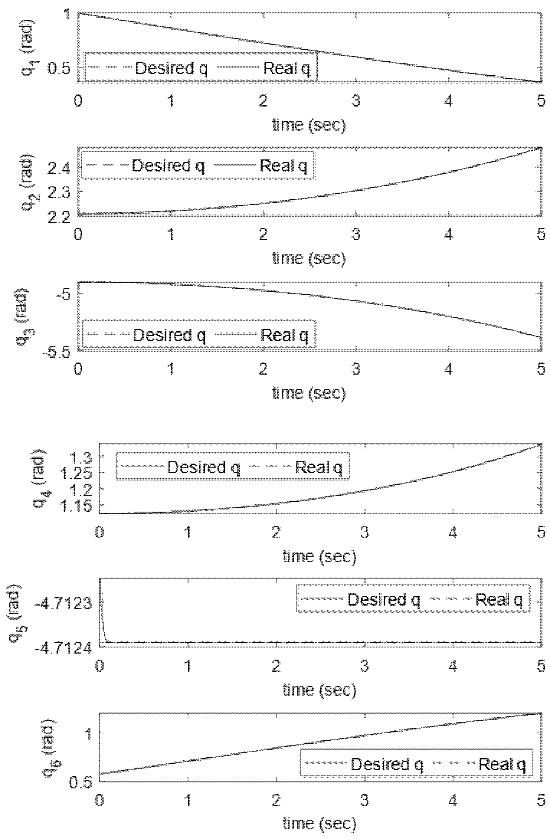
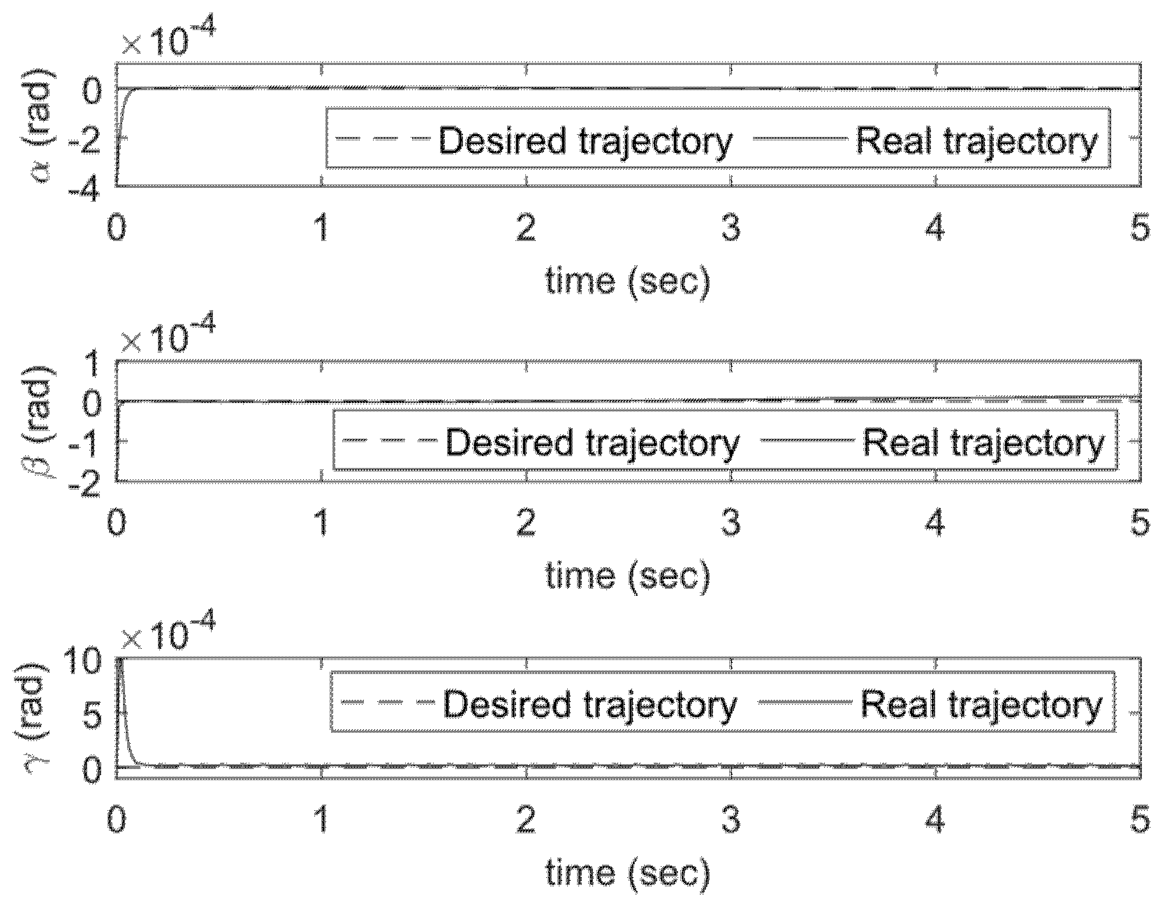
The SMFC is responsible for controlling the robot using the reference joint angles of the robot (see Figure 1). While the maximum applicable torque for the first three joints of UR5 is equal to 150 N.m., it is equal to 28 N.m. for the next three joints. These limitations are due to the motors used to control UR5 by the manufacturer. A maximum of 10% uncertainty is added to each element of $M\left(q\right),C\left(q,\dot{q}\right)\dot{q},\mathrm{and}G\left(q\right)$ used in the controller structure to test its robustness. The time response of the industrial robot in terms of real joint angles versus time is presented in Figure 2. The parameters $q_1,\dots ,q_6$ refer to the joint angles #1–#6 of UR5. As can be seen from the figure, the controller is performing well, and joint angle position errors are very small. The 3D orientation tracking of the UR5 end-effector is illustrated in Figure 3. As can be seen from the figure, the steady-state errors of the industrial robot for $\alpha ,\beta ,$ and $\gamma$ coordinates are small.

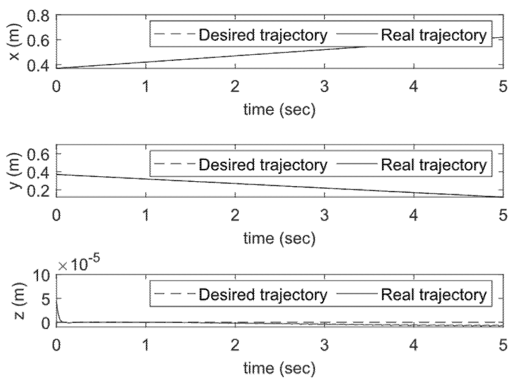
The position tracking of the UR5 is illustrated in Figure 4, which demonstrates a very small tracking error in the UR5 end-effector position.

To have a comparison with a state-of-the-art control algorithm for UR5, the proposed approach is compared with sliding mode control approach, which was previously applied to a UR5 in [39]. The trajectory given for the robot is the same as the one given in [39], as follows:

$$Desiredtrajectory\#2=\{\begin{array}{c}\begin{array}{l}{x}_d=0.37+cos\left(1.26t\right)\\ y_d=0.37+sin\left(1.26t\right)\\ z_d=0.05t\\ {\alpha }_d=0.01\\ {\beta }_d=-1\\ {\gamma }_d=-0.01\end{array}\end{array}$$

(47)

The same controller parameters as in Table 1 are used to track this trajectory. The same maximum 10% uncertainty is added to the elements of $M\left(q\right),C\left(q,\dot{q}\right)\dot{q},\mathrm{and}G\left(q\right)$ used in the controller structure to test its robustness. To find the position error, the overall position error is calculated as the average value of the normed error at each individual sample, using the following equation.

$$||E_p||=\frac{1}{N}{\displaystyle \sum }_{i=1}^N||e_p^i||,$$

(48)

where $e_p^i$ is the individual sample error for position, and $N$ is the total number of the samples. The orientation error is calculated as follows.

$$||E_o||=\frac{1}{N}{\displaystyle \sum }_{i=1}^N||e_o^i-\langle 1,\mathbf{0}\rangle ||$$

(49)

where $e_o^i$, the error for each individual sample, is calculated as $e_o^i=x_{do}^i\otimes {(x_{ro}^i)}^{-1}$, and $\otimes$ and ${(.)}^{-1}$ represent the quaternion product and quaternion conjugate, respectively. Moreover, $x_{do}^i$ and $x_{ro}^i$ represent the desired quaternion and real quaternion orientation of the object. Using the indexes as introduced in Equations (48) and (49), a comparison can be made between the proposed approach and the approach previously introduced in [39]. As presented in Table 2, while $||E_p||$ is equal to 8.255 × 10⁻⁵ m in the case of the proposed approach in this paper, it is equal to 0.0068 m in the sliding mode control approach presented in [39]. This means that the proposed controller in this paper is capable of controlling the UR5 with a considerably lower error value. Moreover, while $||E_o||$ is equal to 2.086 × 10⁻⁴ rad in this paper, it is equal to 0.0035 rad in the sliding mode control approach investigated in [39]. Hence orientational error is considerably lower for the proposed approach.

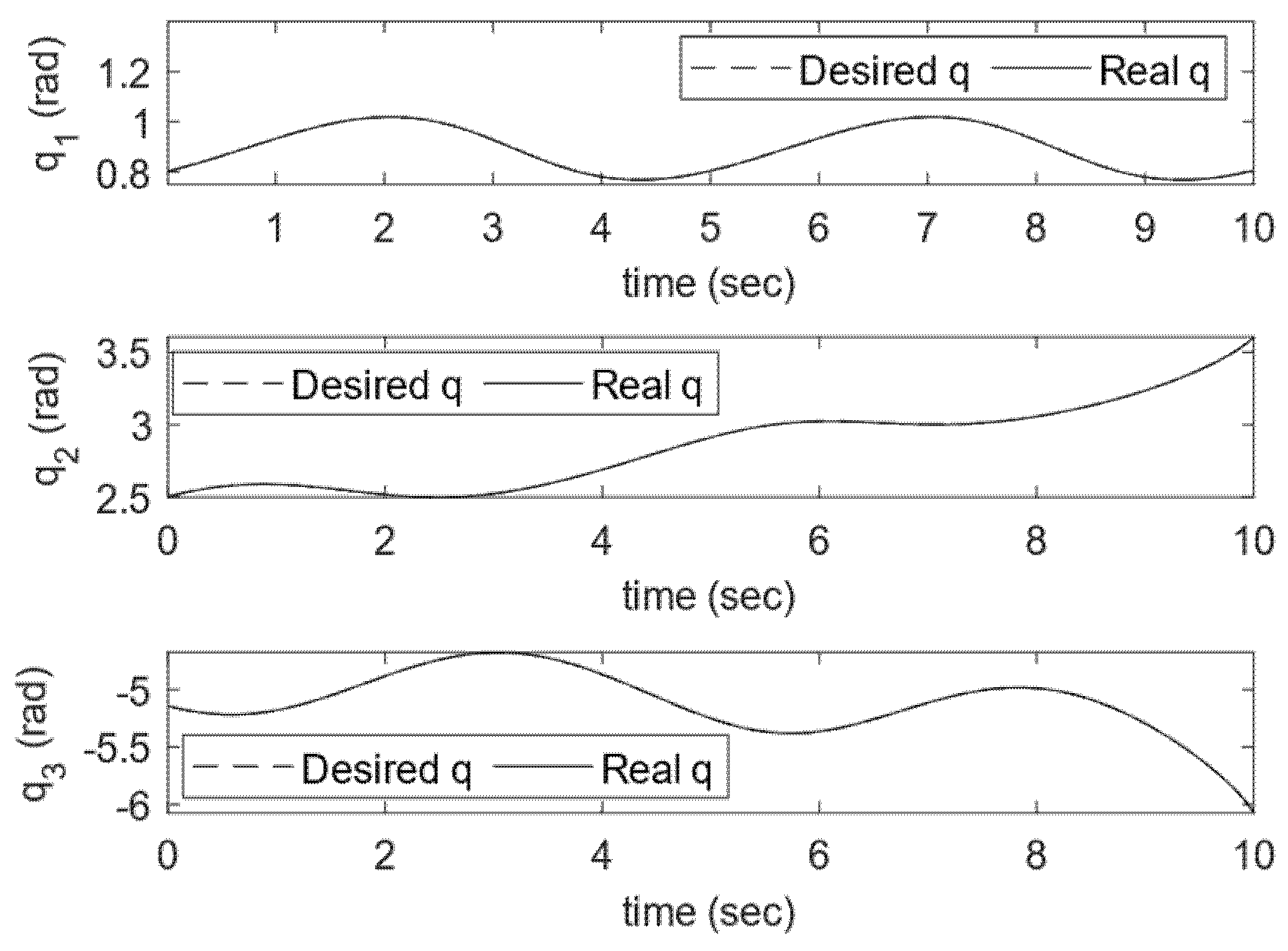
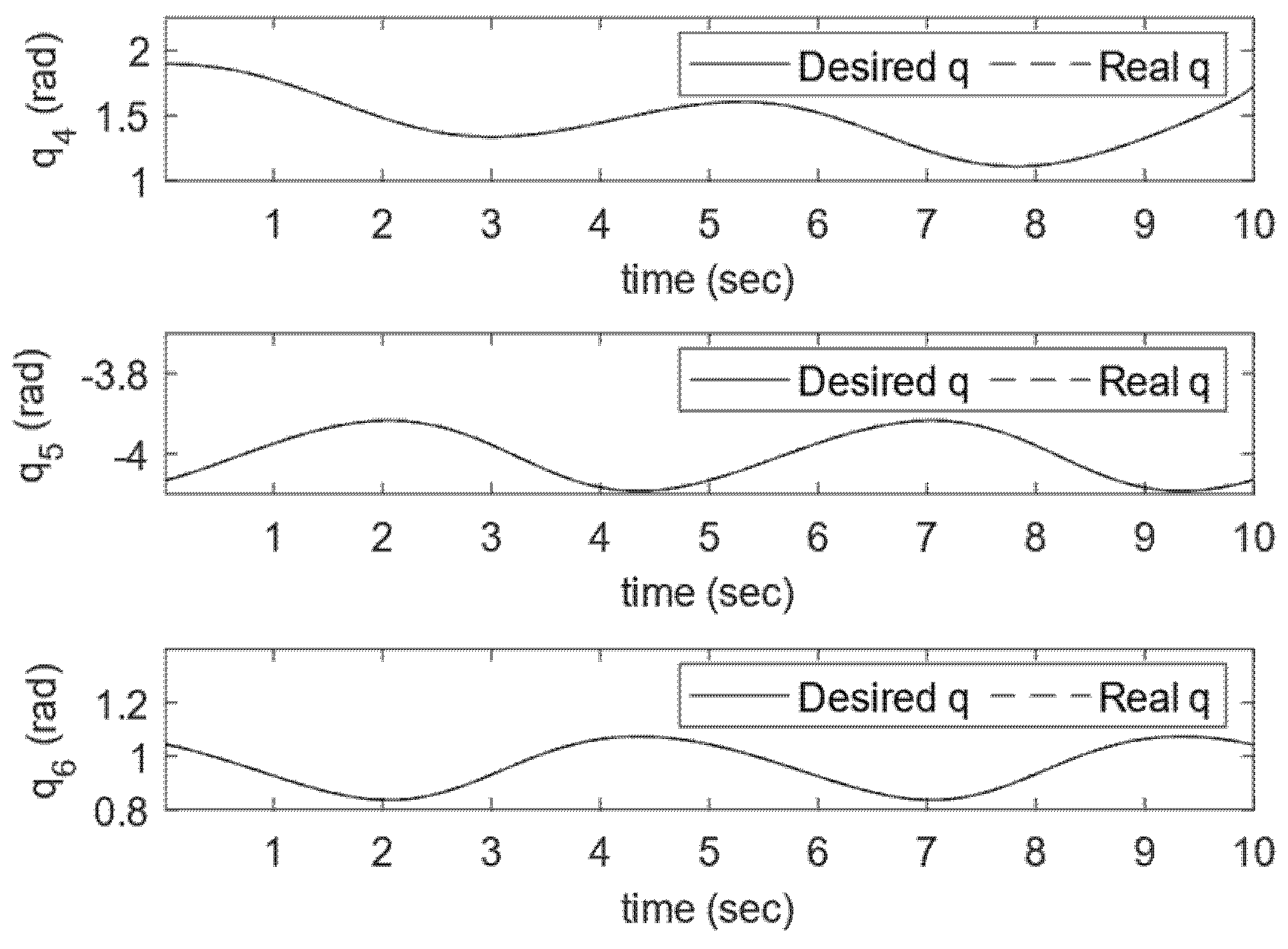
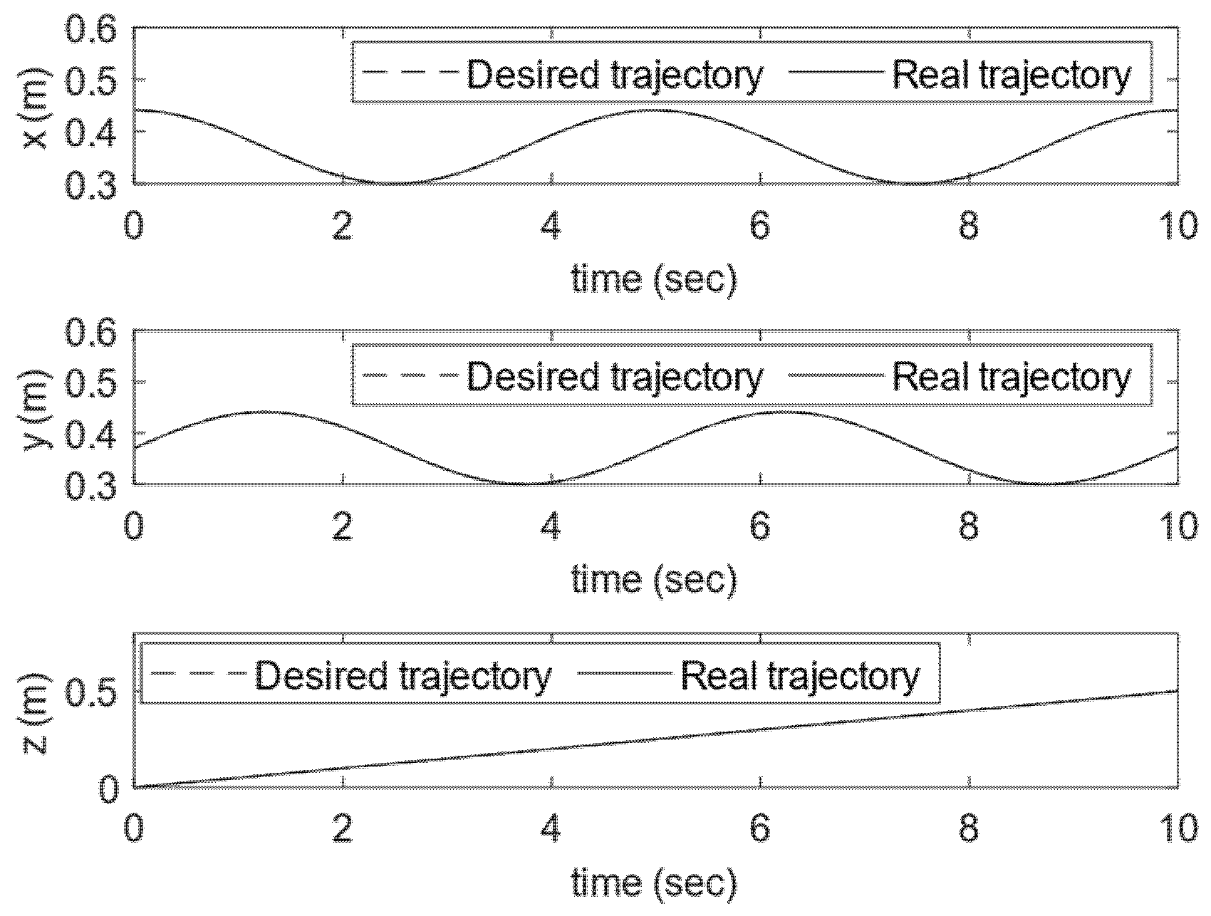
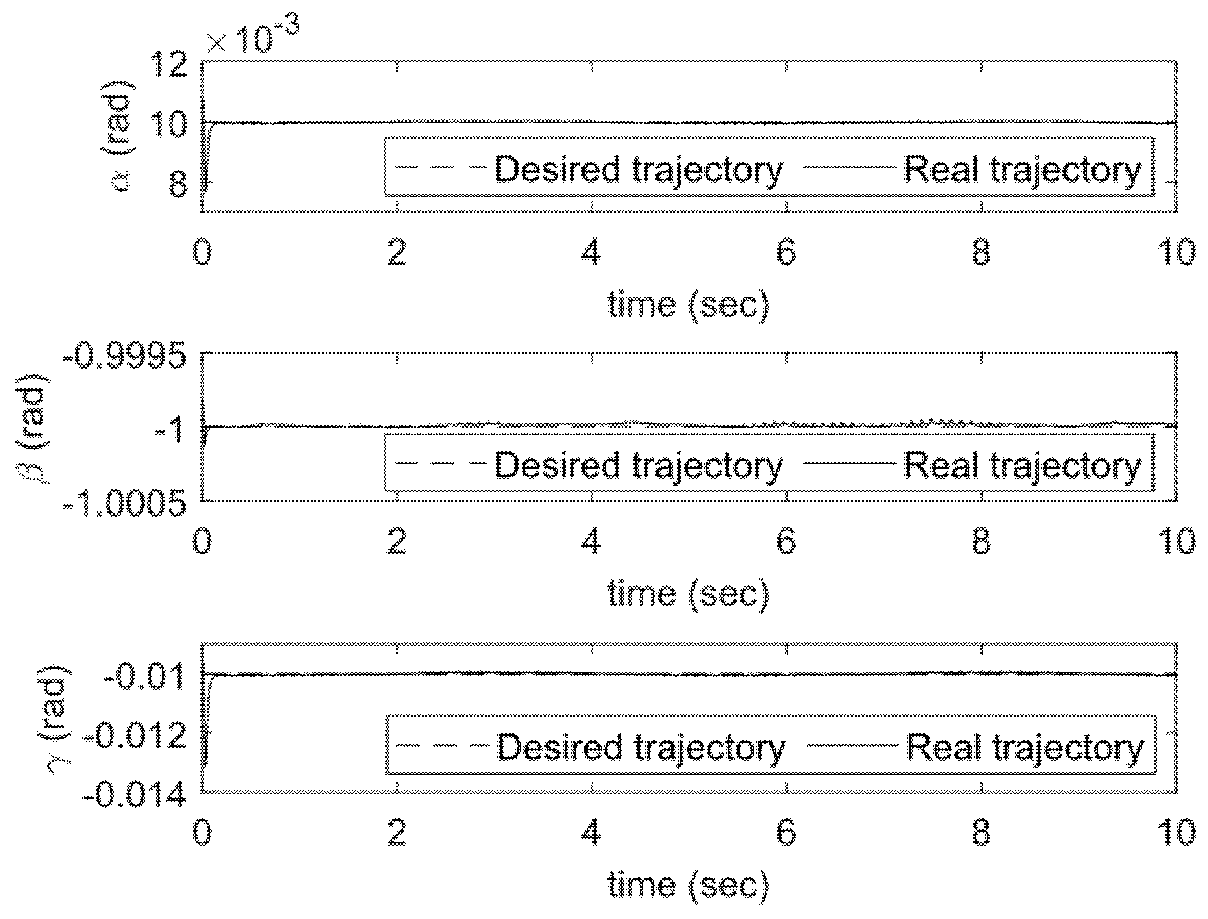
The trajectory tracking of the proposed controller in terms of joint angles is presented in Figure 5 and Figure 6. As can be seen from the figures, the initial conditions of UR5 selected based on the desired trajectory and applying the control law of Equation (28) resulted in the real trajectory for robot joint angles $q$s to be very close to the desired robot joint angles $q_{\mathrm{d}}$s. Moreover, the trajectory tracking performance of the proposed approach in terms of position and orientation is presented in Figure 7 and Figure 8, respectively. The result shows that the desired joint angles are followed with high performance.

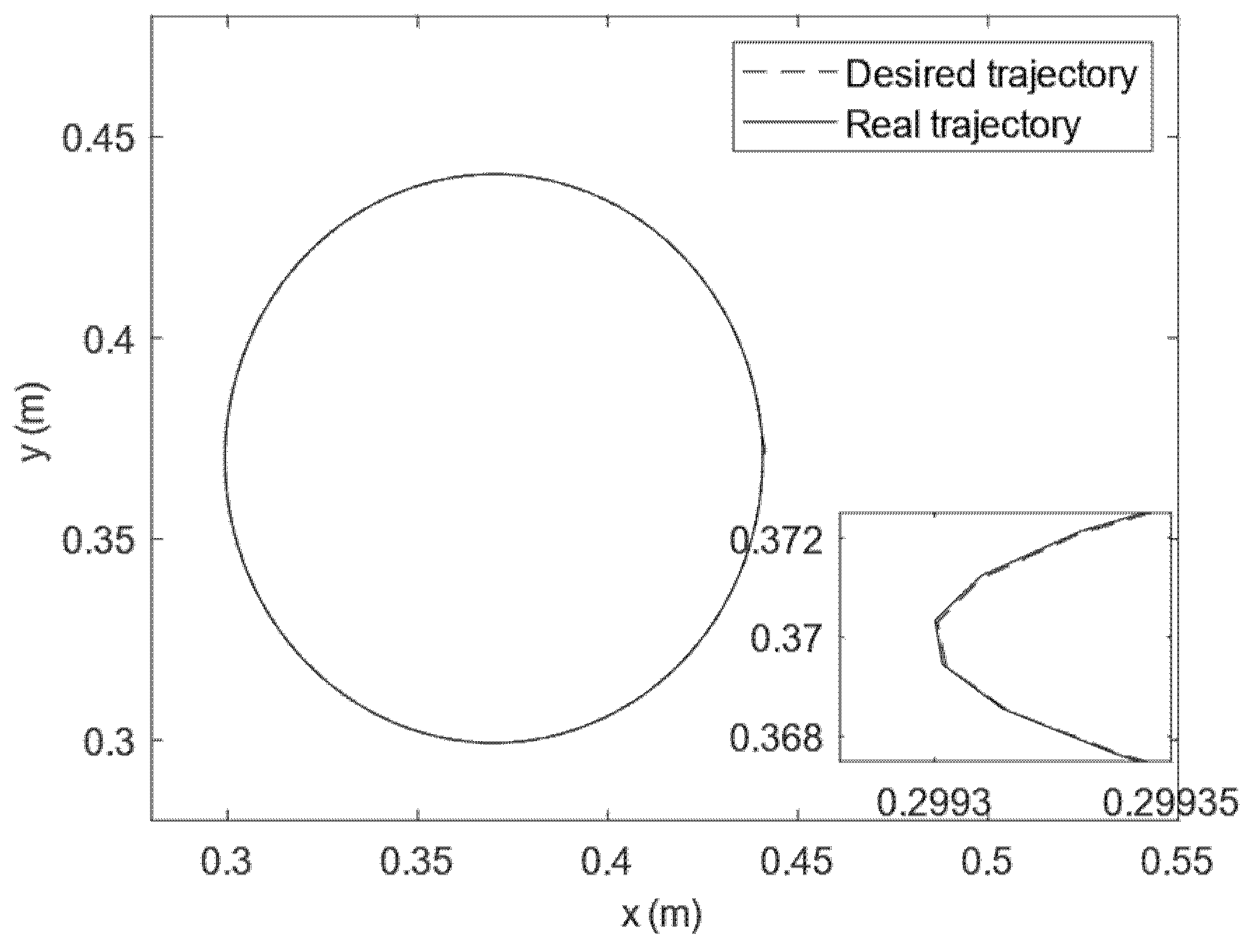
Figure 9 demonstrates the trajectory tracking behavior of UR5 in the xy-plane. For a better comparison between the real trajectory of the robot and its desired values, a zoomed-in version of the graph is presented. This figure shows that the proposed controller is capable of tracking the trajectory defined in Equation (47) with high performance in the presence of dynamic friction and parameter uncertainty. The numerical comparison between the desired Cartesian coordinate and real coordinate of the robot is given in

Table 3. Tacking position and orientation errors in the case of the second trajectory.

Method	$||{\mathit{E}}_{\mathit{p}}||\left(\mathbf{m}\right)$	$||{\mathit{E}}_{\mathit{o}}||\left(\mathbf{rad}\right)$
PD controller [39]	0.0104 m	0.0049
SMC method [39]	0.0068 m	0.0035
The proposed Approach	8.255 × 10−5 m	2.086 × 10−4

.

5. Conclusions

The prominent requirements of an advanced manufacturing environment for precision control of industrial robots motivates the usage of advanced control techniques. Sliding mode controllers have been proven, in particular, to be an ideal control approach to deal with modeling uncertainties. To control an industrial robot in a Cartesian space, it is necessary to translate 3D Cartesian coordinates to desired joint angles values. The EKF inverse kinematic solver is a successful algorithm to deal with the inverse kinematic problems employed in this paper. This inverse kinematic solver has been previously compared, in [29], with the recursive least square method and demonstrated its superior performance. Covariance resetting as a robust modification to the original version of EKF is employed to avoid covariance bursting in its structure. The SMFC approach is responsible for dynamic stabilization and tracking control of the industrial robot. The Lyapunov stability theory is used to analyze the stability of the proposed control structure as well as the adaptation laws for the fuzzy system parameters. Robustness of the controller in the presence of dynamic friction, which inherently exists in the UR5 at low speeds, is analyzed using the same Lyapunov function. The proposed controller is compared with a previous controller investigated in [39] on a UR5 model. It is shown that the proposed controller in this paper outperforms the controller designed in [39] in terms of positional and orientation accuracies. During these simulations, the robustness of the proposed controller against uncertainty in terms of dynamic friction and parameter uncertainties in the UR5 structure is observed. It is shown that the proposed controller is capable of controlling the system with high performance in the presence of uncertainties in a robot model.

6. Future Works

In future, the proposed controller will be implemented on a real robot with an advanced metrology system (WFSI, photogrammetry, IMU, and position-fused sensor system) to measure and control the real-time position of the robot. Comparison of performance to further improved controllers, including ones that use non-quadratic Lyapunov functions, will be considered.

References

- Wanasinghe, T.R.; Gosine, R.G.; James, L.A.; Mann, G.K.I.; de Silva, O.; Warrian, P.J. The Internet of Things in the Oil and Gas Industry: A Systematic Review. IEEE Internet Things J. 2020, 7, 8654–8673. [Google Scholar] [CrossRef]
- Garg, S.; Kaur, K.; Kaddoum, G.; Choo, K.-K.R. Toward Secure and Provable Authentication for Internet of Things: Realizing Industry 4.0. IEEE Internet Things J. 2020, 7, 4598–4606. [Google Scholar] [CrossRef]
- Burnap, P.; Branson, D.; Murray-Rust, D.; Preston, J.; Richards, D.; Burnett, D.; Edwards, N.; Firth, R.; Gorkovenko, K.; Khanesar, M.A.; et al. Chatty factories: A vision for the future of product design and manufacture with IoT. In Proceedings of the IET Conference, Online, 1–2 May 2019; pp. 4–6. [Google Scholar] [CrossRef]
- Lakoju, M.; Ajienka, N.; Khanesar, M.A.; Burnap, P.; Branson, D.T. Unsupervised Learning for Product Use Activity Recognition: An Exploratory Study of a "Chatty Device". Sensors 2021, 21, 4991. [Google Scholar] [CrossRef]
- Slamani, M.; Nubiola, A.; Bonev, I.A. Modeling and assessment of the backlash error of an industrial robot. Robotica 2012, 30, 1167–1175. [Google Scholar] [CrossRef]
- Hoang, M.L.; Carratu, M.; Paciello, V.; Pietrosanto, A. A new Orientation Method for Inclinometer based on MEMS Accelerometer used in Industry 4.0. In Proceedings of the 2020 IEEE 18th International Conference on Industrial Informatics (INDIN), Warwick, UK, 21–23 July 2020; pp. 177–181. [Google Scholar]
- Mishra, D.; Roy, R.B.; Dutta, S.; Pal, S.K.; Chakravarty, D. A review on sensor based monitoring and control of friction stir welding process and a roadmap to Industry 4.0. J. Manuf. Processes 2018, 36, 373–397. [Google Scholar] [CrossRef]
- Ahmadieh Khanesar, M.; Bansal, R.; Martínez-Arellano, G.; Branson, D.T. XOR Binary Gravitational Search Algorithm with Repository: Industry 4.0 Applications. Appl. Sci. 2020, 10, 6451. [Google Scholar] [CrossRef]
- Luo, H.; Zhao, F.; Guo, S.; Yu, C.; Liu, G.; Wu, T. Mechanical performance research of friction stir welding robot for aerospace applications. Int. J. Adv. Robot. Syst. 2021, 18, 1729881421996543. [Google Scholar] [CrossRef]
- Utkin, V.; Guldner, J.; Shi, J. Sliding Mode Control in Electro-Mechanical Systems; CRC press: Boca Raton, FL, USA, 2017. [Google Scholar]
- Lin, J.; Zhao, Y.; Zhang, P.; Wang, J.; Su, H. Research on Compound Sliding Mode Control of a Permanent Magnet Synchronous Motor in Electromechanical Actuators. Energies 2021, 14, 7293. [Google Scholar] [CrossRef]
- Pietrala, M.; Leśniewski, P.; Bartoszewicz, A. Sliding Mode Control with Minimization of the Regulation Time in the Presence of Control Signal and Velocity Constraints. Energies 2021, 14, 2887. [Google Scholar] [CrossRef]
- Khalil, H.K. Nonlinear Control; Pearson: Englewood Cliffs, NJ, USA, 2015. [Google Scholar]
- Slotine, J.J.E.; Li, W. Applied Nonlinear Control; Pearson Education Taiwan: Upper Saddle River, NJ, USA, 2005. [Google Scholar]
- Ullah, S.; Khan, Q.; Mehmood, A.; Bhatti, A.I. Robust backstepping sliding mode control design for a class of underactuated electro–mechanical nonlinear systems. J. Electr. Eng. Technol. 2020, 15, 1821–1828. [Google Scholar] [CrossRef]
- Ullah, S.; Khan, Q.; Mehmood, A.; Kirmani, S.A.M.; Mechali, O. Neuro-adaptive fast integral terminal sliding mode control design with variable gain robust exact differentiator for under-actuated quadcopter UAV. ISA Trans. 2021, 120, 293–304. [Google Scholar] [CrossRef]
- Ullah, S.; Mehmood, A.; Khan, Q.; Rehman, S.; Iqbal, J. Robust integral sliding mode control design for stability enhancement of under-actuated quadcopter. Int. J. Control Autom. Syst. 2020, 18, 1671–1678. [Google Scholar] [CrossRef]
- Liu, Y.; Kong, M.; Wan, N.; Ben-Tzvi, P. A geometric approach to obtain the closed-form forward kinematics of h4 parallel robot. J. Mech. Robot. 2018, 10, 051013. [Google Scholar] [CrossRef] [Green Version]
- Yahya, S.; Moghavvemi, M.; Mohamed, H.A. Geometrical approach of planar hyper-redundant manipulators: Inverse kinematics, path planning and workspace. Simul. Model. Pract. Theory 2011, 19, 406–422. [Google Scholar] [CrossRef]
- Vasilyev, I.; Lyashin, A. Analytical solution to inverse kinematic problem for 6-DOF robot-manipulator. Autom. Remote Control 2010, 71, 2195–2199. [Google Scholar] [CrossRef]
- Lai, Y.-L.; Liao, C.-C.; Chao, Z.-G. Inverse kinematics for a novel hybrid parallel–serial five-axis machine tool. Robot. Comput. Integr. Manuf. 2018, 50, 63–79. [Google Scholar] [CrossRef]
- Jiang, G.; Luo, M.; Bai, K.; Chen, S. A precise positioning method for a puncture robot based on a PSO-optimized BP neural network algorithm. Appl. Sci. 2017, 7, 969. [Google Scholar] [CrossRef]
- Hassan, A.A.; El-Habrouk, M.; Deghedie, S. Inverse kinematics of redundant manipulators formulated as quadratic programming optimization problem solved using recurrent neural networks: A review. Robotica 2020, 38, 1495–1512. [Google Scholar] [CrossRef]
- Jiménez-López, E.; de la Mora-Pulido, D.S.; Reyes-Ávila, L.A.; de la Mora-Pulido, R.S.; Melendez-Campos, J.; López-Martínez, A.A. Modeling of Inverse Kinematic of 3-DoF Robot, Using Unit Quaternions and Artificial Neural Network. Robotica 2021, 39, 1230–1250. [Google Scholar] [CrossRef]
- Lazarevska, E. A neuro-fuzzy model of the inverse kinematics of a 4 DOF robotic arm. In Proceedings of the 2012 UKSim 14th International Conference on Computer Modelling and Simulation, Cambridge, UK, 28–30 March 2012; pp. 306–311. [Google Scholar]
- Wang, X.; Liu, X.; Chen, L.; Hu, H. Deep-learning damped least squares method for inverse kinematics of redundant robots. Measurement 2021, 171, 108821. [Google Scholar] [CrossRef]
- Mohamed, N.A.; Azar, A.T.; Abbas, N.E.; Ezzeldin, M.A.; Ammar, H.H. Experimental Kinematic Modeling of 6-DOF Serial Manipulator Using Hybrid Deep Learning. In Proceedings of the AICV, Cairo, Egypt, 8–10 April 2020; pp. 283–295. [Google Scholar]
- Luo, G.; Zou, L.; Wang, Z.; Lv, C.; Ou, J.; Huang, Y. A novel kinematic parameters calibration method for industrial robot based on Levenberg-Marquardt and Differential Evolution hybrid algorithm. Robot. Comput. Integr. Manuf. 2021, 71, 102165. [Google Scholar] [CrossRef]
- Veitschegger, W.K.; Wu, C.-H. Robot calibration and compensation. IEEE J. Robot. Autom. 1988, 4, 643–656. [Google Scholar] [CrossRef]
- Omodei, A.; Legnani, G.; Adamini, R. Three methodologies for the calibration of industrial manipulators: Experimental results on a SCARA robot. J. Robot. Syst. 2000, 17, 291–307. [Google Scholar] [CrossRef]
- Habibullah, M.; Lu, D.D.-C. A speed-sensorless FS-PTC of induction motors using extended Kalman filters. IEEE Trans. Ind. Electron. 2015, 62, 6765–6778. [Google Scholar] [CrossRef] [Green Version]
- Jiang, Z.; Zhou, W.; Li, H.; Mo, Y.; Ni, W.; Huang, Q. A New Kind of Accurate Calibration Method for Robotic Kinematic Parameters Based on the Extended Kalman and Particle Filter Algorithm. IEEE Trans. Ind. Electron. 2018, 65, 3337–3345. [Google Scholar] [CrossRef]
- Park, I.-W.; Lee, B.-J.; Cho, S.-H.; Hong, Y.-D.; Kim, J.-H. Laser-based kinematic calibration of robot manipulator using differential kinematics. IEEE/ASME Trans. Mechatron. 2011, 17, 1059–1067. [Google Scholar] [CrossRef]
- Hosseinzadeh, M.; Yazdanpanah, M.J. Performance enhanced model reference adaptive control through switching non-quadratic Lyapunov functions. Syst. Control Lett. 2015, 76, 47–55. [Google Scholar] [CrossRef]
- Sun, J.; Xue, X.; Cheng, K.W.E. Fuzzy Sliding Mode Wheel Slip Ratio Control for Smart Vehicle Anti-Lock Braking System. Energies 2019, 12, 2501. [Google Scholar] [CrossRef] [Green Version]
- Khanesar, M.A.; Kayacan, E.; Teshnehlab, M.; Kaynak, O. Extended Kalman Filter Based Learning Algorithm for Type-2 Fuzzy Logic Systems and Its Experimental Evaluation. IEEE Trans. Ind. Electron. 2012, 59, 4443–4455. [Google Scholar] [CrossRef]
- Golouje, Y.N.; Abtahi, S.M. Chaotic dynamics of the vertical model in vehicles and chaos control of active suspension system via the fuzzy fast terminal sliding mode control. J. Mech. Sci. Technol. 2021, 35, 31–43. [Google Scholar] [CrossRef]
- Ovalle, L.; Ríos, H.; Ahmed, H. Robust Control for an Active Suspension System via Continuous Sliding-Mode Controllers. Eng. Sci. Technol. Int. J. 2021, 28, 101026. [Google Scholar] [CrossRef]
- Charaja, J.; Muñoz-Panduro, E.; Ramos, O.E.; Canahuire, R. Trajectory Tracking Control of UR5 Robot: A PD with Gravity Compensation and Sliding Mode Control Comparison. In Proceedings of the 2020 International Conference on Control, Automation and Diagnosis (ICCAD), Paris, France, 7–9 October 2020; pp. 1–5. [Google Scholar]
- Yin, X.; Pan, L. Direct adaptive robust tracking control for 6 DOF industrial robot with enhanced accuracy. ISA Trans. 2018, 72, 178–184. [Google Scholar] [CrossRef] [PubMed]
- Gravdahl, J.T. Force Estimation in Robotic Manipulators: Modeling, Simulation and Experiments. Ph.D. Thesis, Citeseer. NTNU, Trondheim, Norway, 2014. [Google Scholar]
- Kovincic, N.; Müller, A.; Gattringer, H.; Weyrer, M.; Schlotzhauer, A.; Brandstötter, M. Dynamic parameter identification of the Universal Robots UR5. In Proceedings of the ARW & OAGM Workshop, Steyr, Austria, 9–10 May 2019; pp. 44–53. [Google Scholar]
- Kufieta, K. Force Estimation in Robotic Manipulators: Modeling, Simulation and Experiments. In Department of Engineering Cybernetics NTNU Norwegian University of Science and Technology; Norwegian University of Science and Technology: Trondheim, Norway, 2014. [Google Scholar]
- Kebria, P.M.; Al-Wais, S.; Abdi, H.; Nahavandi, S. Kinematic and dynamic modelling of UR5 manipulator. In Proceedings of the 2016 IEEE international conference on systems, man, and cybernetics (SMC), Budapest, Hungary, 9–12 October 2016; pp. 4229–4234. [Google Scholar]
- Chen, Y.; Luo, X.; Han, B.; Luo, Q.; Qiao, L. Model Predictive Control With Integral Compensation for Motion Control of Robot Manipulator in Joint and Task Spaces. IEEE Access 2020, 8, 107063–107075. [Google Scholar] [CrossRef]
- Khanesar, M.A.; Kaynak, O.; Kayacan, E. Sliding-Mode Fuzzy Controllers; Springer International Publishing: Cham, Switzerland, 2021. [Google Scholar]
- Farrell, J.A.; Polycarpou, M.M. Adaptive Approximation Based Control: Unifying Neural, Fuzzy and Traditional Adaptive Approximation Approaches; Wiley: Hoboken, NJ, USA, 2006. [Google Scholar]
- Ioannou, P.A.; Sun, J. Robust Adaptive Control; Courier Corporation: Mineola, NY, USA, 2012. [Google Scholar]
Figure 1.
Overall block diagram of the proposed controller.
Figure 2.
Joint angle behavior of UR5 using the proposed control approach.
Figure 3.
3D orientation behavior of UR5 in the presence of the proposed controller.
Figure 4.
3D position behavior of UR5 in the presence of the proposed controller.
Figure 5.
Trajectory tracking behavior of the robot using the proposed approach for the first three joints.
Figure 6.
Trajectory tracking behavior of the robot using the proposed approach for the last three joints.
Figure 7.
Figure 8.
Figure 9.
3D position behavior of UR5 using the proposed controller in the x-y plane.