Evaluation of Drive Cycle-Based Traction Motor Design Strategies Using Gradient Optimisation

Abstract

In this paper, two design optimisation methods are evaluated using gradient-based optimisation for electric vehicle traction applications. A driving cycle-based approach is used to evaluate specific operational points for the design optimisation procedure. To determine the operational points, an energy centre of gravity (ECG) approach is used. Both optimisation methods are described, namely the point based method and the flux mapping method, with a focus on the flux mapping procedure. Within the flux mapping approach, an inner optimisation loop is defined in order to maintain the stability of gradient calculation for the gradient-based optimisation. An emphasis is placed on the importance of how the optimisation problem is defined, in terms of the objective function and constraints, and how it affects a gradient based optimisation. Based on a design case study conducted in the paper, it is found that the point-based strategy realised motor designs with a slightly lower overall cost (5.66% lower than that of the flux mapping strategy with 8 ECG points), whereas the flux mapping strategy found motor designs with a lower input energy (1.48% lower than that of the point-based strategy with 8 ECG points). This may be attributed to the difference in the definition and interpretation of constraints between these two methods. It is also shown that including more operational points from the driving cycle in the design optimisation leads to designs with reduced total input energy and thus better drive-cycle energy efficiency. This paper further illustrates the significant computational advantages of a gradient-based optimisation over a global optimisation method as it can be completed within a fraction of the time while still finding a global optimum, as long as the problem definition is correctly determined.

1. Introduction

There is a global increase in the use of electrified power trains within the transportation sector. Electric motors are one of the critical components in electric vehicle (EV) power trains. The design of these electric motors can be a challenging task as it involves multiple design considerations such as the efficiency, cost, size, weight, and torque quality or a combination of them [1,2,3,4]. Traditionally, the EV motor design mainly focuses on one or two key working points of the torque–speed envelope [5,6,7]. In recent years, driving cycle-based motor design optimisation, where the efficiency of the machine over the entire driving cycle is considered, has become increasingly popular. Several works have been carried out utilising finite element analysis (FEA) and driving cycle-based techniques to maximise the efficiency of the motor over a driving cycle. In [2], a system level design optimisation is conducted over multiple driving modes for a synchronous reluctance machine, while in [3], a design optimisation is undertaken which optimises the efficiency of the permanent magnet (PM) motor over a given driving cycle. The research conducted in these papers shows the significance of using equivalent working points from the driving cycle analysis, as well as how a design optimisation can be conducted for a driving-cycle based design.

As it is not feasible to optimize a motor design for every speed and torque point of the driving cycle, certain data segmentation and clustering techniques are required. There are many different methods to consider when determining these representative points. In [8], the equivalent representative points from the driving cycle are determined through a centre of gravity means. This method determines these points by breaking the driving cycle up into equivalent grids and using the equivalent centre of gravity for these points over the grid space. With this method, it was shown that an increase in overall efficiency is obtained compared to a key working point optimisation technique. However, this method has also a weakness—i.e., it may not fully encapsulate the primary working points at which the motor operates during the driving cycle.

In [1,9,10,11,12], the energy representative points are defined through an energy center of gravity approach from the driving cycle, which is used to maximise the energy efficiency of an EV’s traction motor over the driving cycle. The energy centre of gravity is similar to the center of gravity method; however, it uses the equivalent energy distribution over the driving cycle instead of the speed–torque points. In [9], the maximum energy efficiency of an EV was defined and presented. A total of 12 equivalent operating points were used from the driving cycle with different energy distributions. The proposed design technique was further validated by a design case and measurement results. In [10], the influences of different driving cycles on design optimisations for PM motors are analysed. From the research conducted, it was shown that for all different driving cycles used, a high efficiency is achieved over a wide torque–speed range. This further proves the validity of the energy center of gravity approach.

In [11], an optimised torque distribution strategy of maximising the motor efficiency for a front and rear-wheel driven EV is described. By using the energy center of gravity method, an understanding was developed of the energy consumption during the low-torque region for a particular driving cycle. In [12], a hybrid approach of combining a data clustering and energy center approach was implemented. It was found in the research that the energy center of gravity and hybrid approaches both converged to similar results, which shows that either can be used when a drive cycle-based optimisation is required. These papers show the validity of the energy center of gravity approach and its use in determining equivalent working points from a driving cycle.

In [4,13], a k-means clustering algorithm is used in order to determine the most relevant points from an energy distribution of the driving cycle. From both papers, the k-means algorithm helped to locate the key areas where the greatest amount of energy is consumed from the driving cycle using a data mining algorithm. This method helps to define the most important working points that the motor operates at compared to a segmented approach. Further, an evaluation is conducted in [1] for different clustering and grouping methods of representative points from the driving cycle. It was shown that by considering these representative operating points, an improved efficiency can be found over a single operating point method. There is clearly an advantage for the drive cycle-based motor design approaches when compared with the traditional design approach.

It is further noted that using different optimisation and design techniques plays a vital role as well. Methods are used where the representative points of the driving cycle are simulated through finite element (FE) analysis, where the specified voltage and current are determined for each particular point. One method that can be taken into consideration is a simple point-based method. DQ currents of the motor for specific operating points are used to determine the output parameters of the motor at specified speed points. These parameters include the voltage, torque, current density, and flux-linkage. This is seen to be one of the easier methods to implement for design techniques. One other method which is considered is the use of flux-linkage mapping. This method simulates a flux-linkage map for a motor design. The map is then searched over in order to find the best operational parameters for the specified operating point [4,10,14,15,16,17]. An area that is not always clear for EV motor designers is the choice of suitable design strategies to use for FEA-based design optimisation procedures. An understanding is required of the differences between the two methods, as well as their respective implementations.

In the above-discussed literature, global optimisation algorithms are almost exclusively used in machine design optimisations, which shows the popularity of the global optimisation algorithms in engineering designs [18]. Despite the advantages of these global optimisation algorithms, they are known to be computationally expensive when compared with their gradient-based counterparts. Gradient-based optimisation has been shown to be more computationally efficient than global optimisation methods, especially when many variables are being considered. Yet, the latter also suffers from finding local minima and its dependence of the starting values of variables [19]. In [20], a gradient-based optimisation was used for a grid-connected wound-rotor induction motor. It was shown that for the gradient based optimisation problem, the gradient-based algorithm needs to be carefully formulated to ensure a global minimum is found. Success was also shown in [21] using gradient-based optimisation; however, only a two-point method was used instead of the full driving cycle analysis. Furthermore, in [22], it was determined that the gradient-based optimisation method used was comparable to a global optimisation solution with the gradient method converging in a faster time.

In this paper, an evaluation is conducted of the two design techniques for traction motors—namely, the point-based design and the flux-linkage map methods—through gradient-based design optimisation. This is conducted in order to show the differences between both design techniques and to help to choose a technique to implement for traction design. Further, this paper shows that gradient-based design optimisation is still an attractive method for traction motor designs as it is computationally efficient and effective in locating a global optimum, provided that the design optimisation is carefully configured. The remaining part of the paper is organised as follows: in Section 2, the driving cycle is analysed and the equivalent representative points are determined. In Section 3, the different design optimisation techniques are elaborated on. In Section 4, an evaluation is conducted for both techniques, and the design and simulation of a case study machine is conducted. Lastly, relevant conclusions are drawn in Section 5.

2. Drive Cycle Analysis

In this section, the motor torque–speed envelope based on the specifications of the studied electric vehicle and the world-wide harmonised light-duty vehicle test procedure (WLTP) drive cycle for a class 3 vehicle is described. The motor energy consumption distribution over the WLTP drive cycle is analysed and is then used to determine certain representative points through clustering techniques. These representative points are important for formulating a drive cycle-based optimisation process.

2.1. Electric Vehicle and Motor Design Specifications

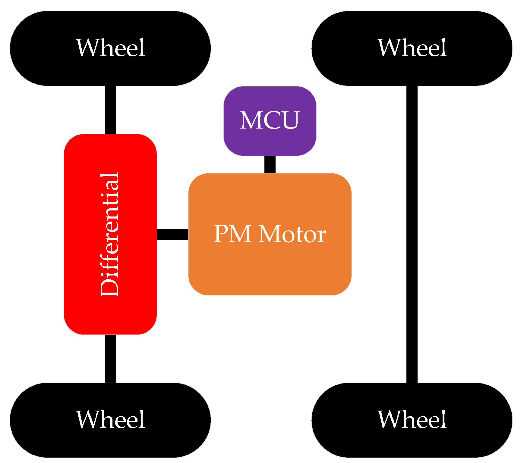
An electric vehicle with the capabilities of being able to operate in suburban areas is investigated for a drive cycle-based optimisation in this paper. The power train topology of the vehicle is shown in Figure 1, where a PM motor is coupled to the front axial of the vehicle via a differential. The power and torque capabilities of the motor are derived through fundamental analytical vehicle load equations, which take into account the vehicle’s resistances and acceleration [23,24]. The specifications and properties of the investigated EV and motor are given in

Table 1. Specifications of proposed EV Design.

	Parameters	Value
Electric	Wheel radius (m)	0.27
Vehicle	Vehicle frontal area (m ${}^2$)	2.5
	Aerodynamic drag coefficient ($C_d$)	0.3
	Rolling resistance coefficient ($C_r$)	0.013
	Vehicle mass (kg)	1000
	Differential gear ratio	6:1
	Maximum vehicle speed (km/h)	131.3

, with wind resistance being regarded as negligible for this case study.

2.2. Determining Representative Points from the Driving Cycle

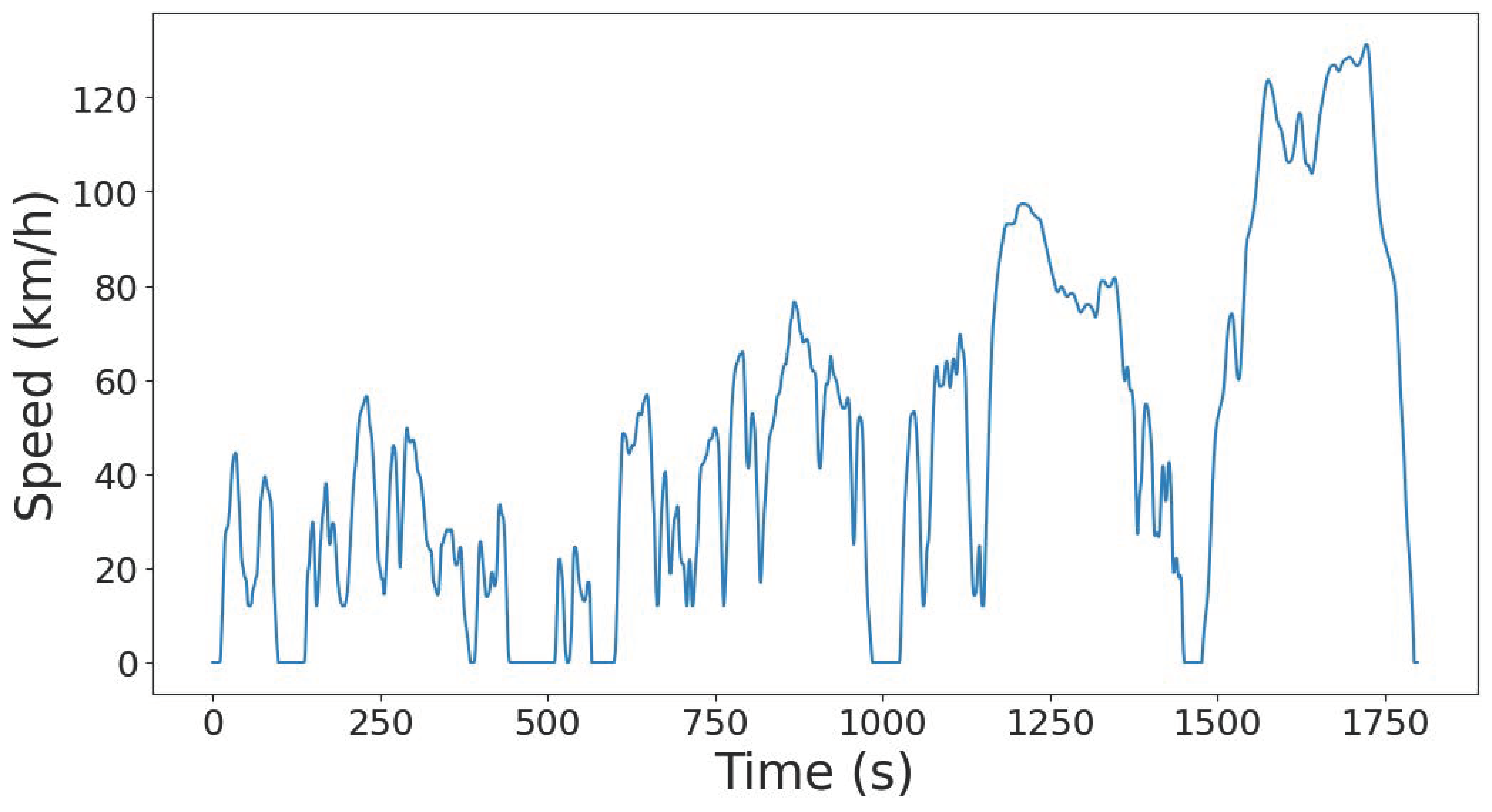
The torque and speed demand required by the vehicle is analysed over the WLTP drive cycle. This driving cycle procedure is predominately used to measure fuel consumption, CO ${}_2$ emissions, pollutant emissions, and the energy consumption of alternative power trains such as electric vehicles [25]. The driving cycle has a duration of 1800 s, with a distance of 23,266 m. The driving cycle is divided up into four different sub-systems, with each simulating an urban, suburban, rural, and highway driving scenario, respectively. The maximum speed required by the cycle is 131.3 km/h. The speed profile of the WLTP is shown in Figure 2.

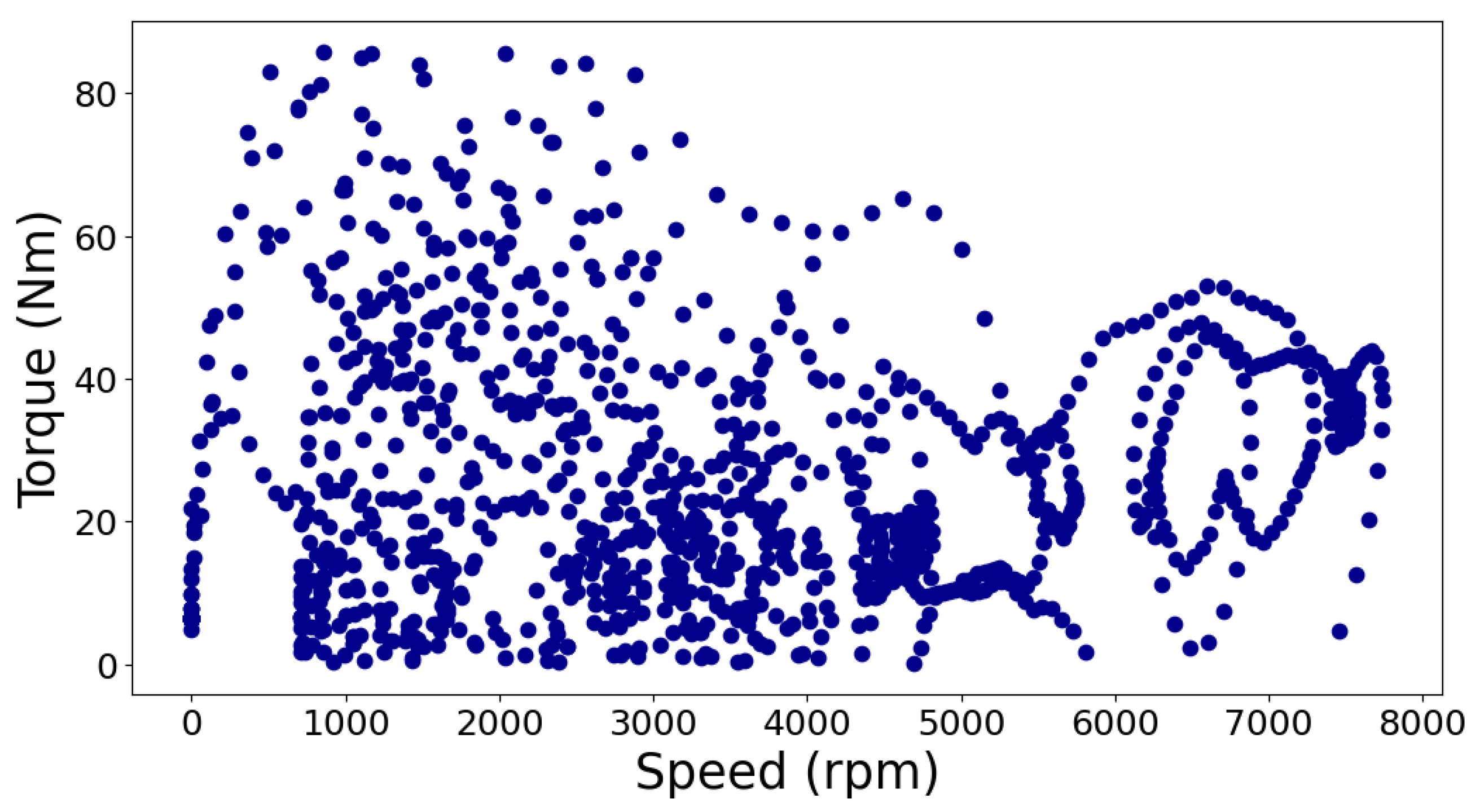
Using the vehicle dynamics model in [23,24], the required traction efforts for the given wheel radius and differential gear ratio can be determined [3,8]. The torque requirements over the driving cycle range can be readily calculated and mapped as shown in Figure 3. As the motor is designed and optimised for motor operation, regenerative braking is not considered. The torque distributions over the entire motor speed range (constant torque and constant power) for the WLTP driving cycle are given in Figure 4.

Several different methods are used to determine the representative operating points from a driving cycle for the design optimisation process. In [8,26], the geometric center of gravity method is used, which is based on the geometric representation of torque distribution points within an area of the driving cycle. Essentially, this method focuses on the greatest amount of time for which the motor operates within a given area specified by the user. Another method used to determine the operating points for a driving cycle is the use of the distribution of energy consumed during a driving cycle. Figure 5 shows the energy load profile of the motor in joules, which is determined from the product of torque and speed in Figure 4 over a time period for each torque and speed point. Determining the representative points from the load energy distribution can be done in multiple ways. In [1,9,10,11,12,27], the energy center of gravity (ECG) method is used, which is based on the energy distribution of points within a region of the driving cycle. This method considers the amount of energy used within each region and the weight of the energy for the representative points. Another method is the use of clustering methods. Different types of clustering techniques can be used in order to determine the representative points [1,4,12,13,28]. An evaluation of different methods of choosing the representative points and their respective impact on the design optimisations is reported in [1,12].

For this study, the ECG method is used. The load energy density of the drive cycle is divided up into i clusters. The energy, $E_i$, of the ith cluster or region is calculated as

$$E_i=\sum _{j=1,2\dots }^{N_i}{E}_{j,i}$$

(1)

where $N_i$ is the number of operating points within each ith cluster and j is the number of clusters chosen. The calculated representative torque and speed points within each region, $T_{eq,i}$ and ${\omega }_{eq,i}$, are given as follows:

$$T_{eq,ij}=\frac{1}{E_i}\sum _j^{N_i}{E}_{ij}{T}_{ij}$$

(2)

$${\omega }_{eq,i}=\frac{1}{E_i}\sum _{j=1}^{N_i}{E}_{ij}{\omega }_{ij}$$

(3)

In order to account for the magnitude of each representative point calculated, a weighting factor is required for the optimisation design. These weighting factors are determined according to the amount of required energy during the driving cycle process. These weighting factors of the representative points are calculated according to the ratio of energy consumed by all the operating points during the driving cycle, given as [1]

$$W_{E,i}=\frac{E_i}{{\sum }_{k=1,2\dots }{E}_k}$$

(4)

where k is each operating point of the drive cycle. By using Equations (1)–(4) and specifying the number of clusters to be 8, the representative points shown in Figure 6 are defined in

Table 2. Summary of representative points.

Region	Point	Weighting of Energy ${\mathit{W}}_{\mathit{E}}$
0–2000 rpm 0–42.8 Nm	1345.9 rpm 26.01 Nm	4.64%
0–2000 rpm 42.8–85.8 Nm	1351 rpm 60.1 Nm	10.15%
2001–4000 rpm 0–42.8 Nm	3182.5 rpm 24.69 Nm	20.93%
2001–4000 rpm 42.8–85.8 Nm	2806.6 rpm 56.27 Nm	15.1%
4001–6000 rpm 0–42.8 Nm	4861.8 rpm 26.02 Nm	14.36%
4001–6000 rpm 42.8–85.8 Nm	4601.7 rpm 53.5 Nm	5.88%
6001–8000 rpm 0–42.8 Nm	7014.1 rpm 29.42 Nm	19.42%
6001–8000 rpm 42.8–85.8 Nm	6897.2 rpm 44.48 Nm	9.53%
Base Speed Maximum Torque	3000 rpm 118.7 Nm	N/A
Maximum Speed Torque	8000 rpm 44.5 Nm	N/A

. The motor parameters can be deduced and are given in

Table 3. Specifications of proposed motor design.

Parameters	Value
Nominal power (kW)	37.28
Motor base speed (r/min)	3000
Motor maximum speed (r/min)	8000
Maximum torque (maximum speed) (Nm)	44.5
Peak torque (base speed) (Nm)	118.7
CPSR	2.66

.

3. Design Optimisation Procedure

The motor topology considered for this study is a 24-slot, 8-pole V-shaped interior permanent magnet (IPM) machine. For the finite element based design, a parametric 2D model is shown in Figure 7 with the relevant design parameters that are used for the design optimisation. For each design consideration, a rather conservative slot fill factor of 0.35 is assumed with the temperature of the stator windings and the PM being 120 ${}^{\circ }$C and 80 ${}^{\circ }$C, respectively. Further, given the power rating and the space constraints of the motor, the maximum current density allowed is set to be 10 A/mm${}^2$ in the design, which means that the motor is required to be water cooled. More detailed motor design specifications are tabulated in

Table 4. Motor design specifications.

Parameters	Value
Number of pole pairs	4
Number of slots	24
Air-gap length	1 mm
Winding fill factor	0.35
Lamination steel	M19_26G
PM material and grade	NdFeB N48H
Maximum Line voltage	310  V
Maximum phase current	75  A
Maximum current density	10 A/mm${}^2$

.

To evaluate the motor capabilities for the optimisation procedures, the torque and voltage are required for each operating point as given by (5)–(7), where $v_d$, $v_q$, $i_d$, $i_q$, $L_d$, and $L_q$ are the d and q-axis voltages, currents, and inductances, respectively, $R_s$ is the phase resistance, ${\lambda }_{PM}$ is the PM’s flux-linkage, ${\omega }_e$ is the electric angular speed, p is the number of pole pairs, and $T_e$ is the electromagnetic torque, as described in [29].

$$T_e=\frac{3}{2}p[{\lambda }_{PM}+(L_d-L_q)i_d]i_q$$

(5)

$$v_d=R_s{i}_d-{\omega }_e{L}_q{i}_q$$

(6)

$$v_q=R_s{i}_q+{\omega }_e(L_d{i}_d+{\lambda }_{PM})$$

(7)

Further, in order to calculate the efficiency of all the representative points of the driving cycle, Equations (8)–(10) can be used, where the windage and friction losses are not considered. The core losses ($P_{core}$) in Equation (9) are computed by employing time-step FE solutions and the Steinmetz-based equation [30]. The copper losses are calculated using the finite element mesh in the copper area on a per element basis.

$$P_{copper}=\sum _{e=1}^n\frac{J^2{k}_f{A}_{e}L(1+k_{ew})}{\sigma }$$

(8)

where n is the number of elements in the copper area, J is the RMS current density, $k_f$ is the copper fill factor, $A_e$ is the area of element e, L is the active stack length of the machine, $k_{ew}$ is the ratio of end-winding length to stack length, and $\sigma$ is the conductivity of copper.

$$\eta =\frac{T_e·\omega }{T_e·\omega +P_{copper}+P_{core}}$$

(9)

$${\eta }_{eng}=\sum _{i=1}^N{\eta }_i·{\omega }_{eq,i}$$

(10)

By using the ${\eta }_{eng}$ value as the average efficiency, which takes into account the weighting of energy, and ensuring a constraint is added to this, an overall high efficiency can be maintained for the motor’s operating range. Within the optimisation methods discussed further, the minimum constraint of ${\eta }_{eng}$ is chosen to be 94% due to the allowed cooling capabilities and loss restrictions for the specified case study motor.

3.1. Optimisation Strategies

The optimisation algorithm used within each method of this study is the sequential least squares programming algorithm (SLSQP) [31], which is a gradient-based optimisation method. The SLSQP algorithm minimises a single objective function of multiple variables, subject to both equality and inequality constraints. Both optimisation strategies implemented are conducted using an in-house 2D FE package. Although gradient-based algorithms are more efficient than global methods for electrical machine design with many design variables, they are susceptible to becoming trapped into a local optimum and numerical noise [32]. While the former can be mitigated by using different starting points, the latter can still affect the accuracy and stability of the gradient evaluation for gradient-based optimisation. For this study, a unique implementation of a gradient-based optimisation procedure is applied, which employs a mesh reshaping technique described in [33]. This technique shows significant improvements on the performance of gradient-based optimisation, as it helps with the stability of the gradient calculation while maintaining the mesh quality over a large design space.

3.1.1. Point Based Optimisation Strategy

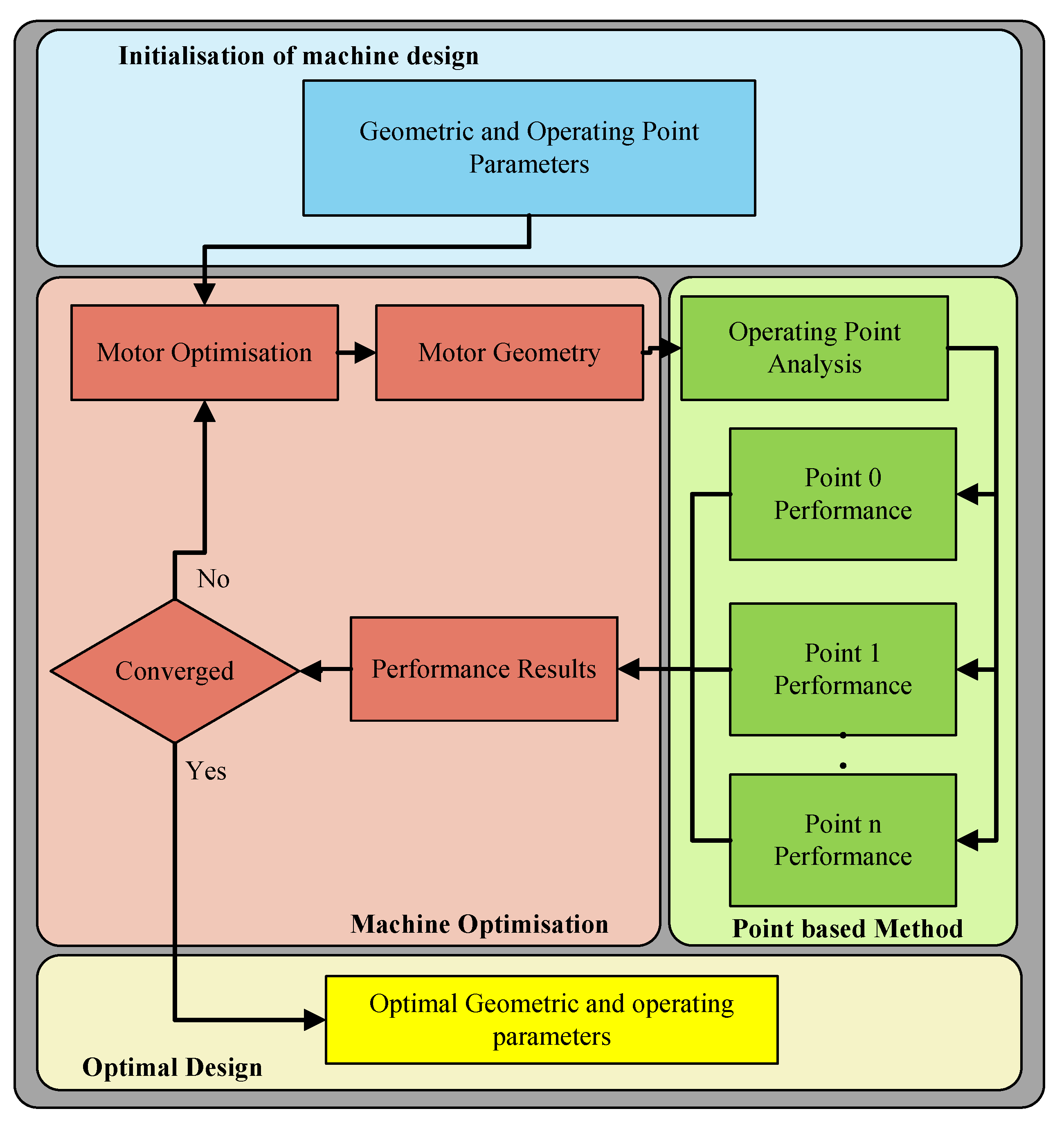
The first optimisation method considered is the point-based optimisation strategy. This method evaluates the motor design along $-n$ points specified from the driving cycle. By evaluating the motor along these design points, it ensures the motor is within the constant power speed range (CPSR) limits set by the user. The motor design is evaluated through an optimisation loop which adjusts both the rotor and stator geometric variables, as well as the dq-currents at each operating point, inherently adjusting the optimal current angle. This process is shown in Figure 8. This method begins by the user setting the initial geometric and operating point parameters. The geometric parameters are given boundaries, and constraints are assigned to the operating point parameters. It is possible to include a relatively large number of design points in the optimisation loop within an efficient time span.

The optimisation problem is formulated as

$$\begin{array}{cc}\hfill \mathrm{Minimise}:& F\left(\mathbf{X}\right)=C_{\mathrm{total}}\hfill \\ \hfill \mathrm{Subject}\mathrm{to}:& T_x\ge T_{min}\left(\mathrm{Nm}\right)\hfill \\ \hfill & V_{LLx}\le V_{max}\left(\mathrm{V}\right)\hfill \\ \hfill & I_{\varphi x}\le I_{max}\left(\mathrm{A}\right)\hfill \\ \hfill & {\eta }_{\mathrm{eng}}\ge {\eta }_{engmin}\hfill \\ \hfill & B_{MMx}\ge B_{max}\left(\mathrm{T}\right)\hfill \\ \hfill & J_x\le J_{max}(\mathrm{A}/\mathrm{mm}{}^2)\hfill \end{array}$$

(11)

where $\mathbf{X}$ represents the vector of design variables, which includes the geometric variables and $dq$-currents for each operating point of the machine. $C_{\mathrm{total}}$ is the cost of the active material of the machine, which includes PM material, copper, and steel. The costs of materials used are given in

Table 5. Costs of materials.

Material	Cost
PM	$50/kg
Silicon steel	$2/kg
Copper	$6.67/kg

. T ${}_{min}$ is the minimum torque for each operating point, $V_{LLx}$ and $I_{\varphi x}$ are the maximum allowable voltage and current for each operating point, respectively, $B_{MMx}$ is the demagnetisation margins of the magnets at each operating point, and $J_{max}$ is the maximum current density allowed. The intrinsic value of this method is the rapid computational time when few points are selected from the driving cycle, as well as the simplicity of the optimisation process.

3.1.2. Flux Mapping Optimisation Strategy

The second optimisation strategy considered is the flux mapping strategy. The process of using flux maps for the optimisation is where the flux linkages on the $dq$-axis are formulated across multiple points, and an interpolation of these points is mapped out. The flow diagram of this method is shown in Figure 9 and Figure 10. A single geometric design is evaluated over multiple points set by the user, similar to the point-based method. However, a look up map of the entire $dq$-parameters is generated. The formulation of a flux map is seen to be less computationally efficient compared to the point-based method due to each $dq$-current point being simulated. However, it has the advantage of the algorithm determining the best fit current curve for each geometric design on all operating points specified, known as the maximum torque per ampere (MTPA) curve. This further allows the user to discern the full capabilities of the motor. An example of the d- and q-axis flux-linkage map of a motor design is shown in Figure 11, which is used to determine the torque map in Figure 12.

In order to evaluate the MTPA on the flux map for each of the operating points, the SLSQP is used once more. This method searches along the flux map while keeping to the specifications set for the $dq$-currents, as shown in Figure 10. The bound and constraints for each operating point on the outer optimisation loop (where the geometric parameters of the machine are optimised) are defined as

$$\begin{array}{cc}\hfill \mathrm{Minimise}:& F\left(\mathbf{X}\right)=C_{\mathrm{total}}\hfill \\ \hfill \mathrm{Subject}\mathrm{to}:& T_x\ge T_{point}\left(\mathrm{Nm}\right)\hfill \\ \hfill & V_{LLx}\le V_{max}\left(\mathrm{V}\right)\hfill \\ \hfill & I_{\varphi x}\le I_{max}\left(\mathrm{A}\right)\hfill \\ \hfill & {\eta }_{\mathrm{eng}}\ge {\eta }_{engmin}\hfill \\ \hfill & B_{MMx}\ge B_{max}\left(\mathrm{T}\right)\hfill \\ \hfill & J_x\le J_{max}(\mathrm{A}/{\mathrm{mm}}^2)\hfill \end{array}$$

(12)

where $\mathbf{X}$ represents the vector of design variables of the machine. $T_{point}$ is the minimum torque for each operating point.

For the inner optimisation loop, where the operating point is evaluated according to the MTPA point on the flux map, the optimisation problem is formulated as

$$\begin{array}{cc}\hfill \mathrm{Minimise}:& F\left(\mathbf{X}\right)=I_{\varphi }\left(\mathrm{A}\right)\hfill \\ \hfill \mathrm{Subject}\mathrm{to}:& T_x\ge T_{point}\left(\mathrm{Nm}\right)\hfill \\ \hfill & V_{LL}\le V_{max}\left(\mathrm{V}\right)\hfill \end{array}$$

(13)

where $\mathbf{X}$ represents the vector of the $dq$-currents as well as the constant of the specified speed for the evaluated operating point. $T_x$ is the set torque value for each operating point. By finding the MTPA point, the output parameters and $dq$-currents are returned to the outer optimisation loop for the geometric design, as shown in Figure 9 and Figure 10.

However, during the design optimisation process, certain outcomes may arise during the outer optimisation process. When a design with certain geometric parameters is simulated, various parameters, such as $V_{L{L}_x}$, may not be within the constraints of $V_{max}$ for any $dq$-currents specified. This may occur when the magnet thickness is sizeable and a large flux linkage is evident. This generates a significant back-EMF in the motor. From this, the inner optimisation algorithm (MTPA) may not able to satisfy the constraints being violated for these points, which either results in the optimisation algorithm failing and terminating or resulting in large gradients occurring during the outer optimisation loop. This further causes the gradient-sensitive optimisation to be incapable of finding the correct minimum cost. In [17], the voltage constraints were handled by formulating an optimisation objective function using Lagrange multipliers. However, the applied on–off gate function may negatively impact the accuracy and stability of the gradient calculations, which is not ideal for gradient-based optimisations. To ensure that the objective and constraints are relatively smooth functions, an optimisation inner-loop shown in Figure 10 has been formulated to deal with these non-convergence cases; i.e.,

$$\begin{array}{cc}\hfill \mathrm{Minimise}:& F\left(\mathbf{X}\right)={\alpha }^2\hfill \\ \hfill \mathrm{Subject}\mathrm{to}:& V_{LL}\le V_{L{L}_{max}}{(1+\alpha )}^2\left(\mathrm{V}\right)\hfill \\ \hfill & T_x\ge T_{point}\left(\mathrm{Nm}\right)\hfill \\ \hfill & I_{\varphi }\le I_{max}\left(\mathrm{A}\right)\hfill \end{array}$$

(14)

where $\mathbf{X}$ represents the vector of the $dq$-currents, as well as the constant of the specified speed for the evaluated operating point. $\alpha$ is chosen as a variable parameter that adjusts the maximum voltage constraint during each iteration of the optimisation loop. During the inner optimisation loop search across the flux map, the constraints given may be violated. From here, this variable parameter is adjusted, which shifts the maximum voltage of the design. Therefore, the constraints may be further improved with each iteration, until a valid design is found. The objective of this optimisation is still tasked with minimising the current on the flux map subject to the constraints; however, the added parameter is also required to be set at a minimum to ensure that the voltage constraint is not overly inflated. This allows the outer optimisation loop to have a smoother gradient for each iteration where a non valid design is found, which improves the gradient-based optimisation of the SLSQP.

4. Evaluation of Optimisation Strategies

A summary of the optimisation results for different numbers of ECG points is given in

Table 6. Evaluation of optimisation method results.

Number of ECGs	Parameters	Multi-Point	Flux Mapping
2	Total cost ($)	108.26	109.2
	Total mass (kg)	21.57	21.83
	PM mass (kg)	0.726	0.771
	Copper mass (kg)	6.48	6.11
	Steel mass (kg)	14.36	14.95
4	Total cost ($)	108.21	115.94
	Total mass (kg)	26.87	24.09
	PM mass (kg)	0.604	0.881
	Copper mass (kg)	5.45	5.46
	Steel mass (kg)	20.81	17.75
6	Total cost ($)	108.62	111.83
	Total mass (kg)	21.59	23.965
	PM mass (kg)	0.748	0.735
	Copper mass (kg)	6.32	6.13
	Steel mass (kg)	14.51	17.1
8	Total cost ($)	106.23	112.42
	Total mass (kg)	23.93	25.66
	PM mass (kg)	0.61	0.63
	Copper mass (kg)	6.26	6.66
	Steel mass (kg)	17.06	18.37

. For each design variation that is developed with different ECG points, the base speed and maximum speed points are also required to be evaluated to ensure that the correct operating parameters are able to be reached. From the results of Table 6, it is seen that the multi-point method generally has a better output result in terms of the objective function of costing when compared to the flux mapping method, with a note regarding the difference in cost for 8 ECG points, with the multi-point method being $5.66\%$ less than the flux mapping method. The number of ECG points included in the optimisation has a greater influence on the optimum results from the flux mapping method than those from the multi-point method.

Figure 13, Figure 14, Figure 15 and Figure 16 show the efficiency maps of the optimum designs, with two ECGs and eight ECGs for both optimisation methods. It is evident that the more ECG points are added, the greater the increase in the overall efficiency range. The flux mapping method has a slightly better performance in terms of the efficiency range for both two ECG and eight ECG cases. This is further elaborated upon in

Table 7. Comparison of drive-cycle energy consumption of the optimum motor designs.

Number of ECGs	Multi-Point	Flux Mapping
2	16.934 GJ	16.882 GJ
4	16.931 GJ	16.793 GJ
6	16.931 GJ	16.778 GJ
8	16.921 GJ	16.673 GJ

, which shows that the drive cycle energy consumption for the designs generated from the flux mapping method is invariably lower than that of the multi-point designs. The difference for the flux mapping method for two ECG points and eight ECG points is a reduction in total input energy by $1.25\%$, whereas for the multi-point method, it is only $0.07\%$. In contrast, the flux mapping method with eight ECG points is $1.48\%$ lower in terms of the total input energy for the eight ECG points. The total input energy given is determined by taking all the points of the driving cycle in Figure 5, and determining from the MTPA algorithm an efficiency map and the efficiency at each point. The total output energy from Equation (1) is used and the corresponding efficiency is incremented, allowing the total input energy required to be given. A pseudo-code is shown in Figure 17 of this process.

The reason that the flux mapping method realises more globally efficient designs when more ECG points are used may be explained as follows. For the multi-point method, the $dq$-currents are specified as variables in the optimisation loop. If these currents satisfy a constraint for an operating point, the optimisation determines this to be valid. This results in the optimisation finding a minimum costing machine, but not necessarily at the MTPA for each operating point. Further, the global ${\eta }_{eng}$ constraint defined is determined intrinsically by the $dq$-currents. This therefore means that if the constraint is met through the optimisation, the most optimal energy efficiency may not be found, but the ideal costing will be. For the flux mapping method, the MTPA for each operating point is determined. This causes the total input energy to be lower compared to the multi-point method, as the MTPA $dq$-current points are optimally determined for each iteration cycle. This leads to a more globally efficient machine design, but not necessarily the lowest-cost design.

The cross-sections of the optimum designs from both the multi-point and flux mapping methods with two ECG points and eight ECG points are shown in Figure 18 and Figure 19. Their respective optimised motor geometric parameters are summarised in

Table 8. Comparison of multi-point and flux mapping optimum designs with two and eight ECG points.

Parameter	Number of ECGs: 2		Number of ECGs: 8
	Multi-Point	Flux Mapping	Multi-Point	Flux Mapping
S1 (mm)	2.79	2.81	2.76	2.81
S2 (mm)	6.1	6.22	7.34	7.55
S3 (mm)	31.13	30.17	24.74	25.8
S4 (mm)	13.85	14.49	14.63	15.53
S5 (mm)	7.29	7.24	9.09	9.33
V1 (mm)	6.98	6.16	4.17	4.28
V2 (mm)	0.5	0.5	0.5	0.78
V3 (mm)	42.98	42.72	55.33	57.1
V4 (mm)	22.37	22.94	39.24	36.98
V5 (mm)	7.55	6.7	2.94	3.54
V$\theta$${}^{\circ }$	115.51	115.1	114.8	114.61
R (mm)	137.14	136.17	151.6	156.07
L (mm)	45.43	46.82	40.33	40.73
Coil turns	12	12	11	11

. Clearly, the optimum designs obtained from both methods are very similar to each other.

Figure 20 displays the computational time of both multi-point and flux mapping methods with different numbers of ECG points. It is observed that for the multi-point method, there is an increase of 8 times in time from 2 ECG points to 8 ECG points, whereas the flux mapping method only has an increase of $1.5$ times. Further, for 8 ECG points, the multi-point method took up to 7397 s whereas the flux mapping method took 3028 s. This shows that the flux mapping method has the potential of being $2.4$ times faster than the multi-point method when many ECG points are used. In order to show the rationale of selecting the gradient-based design optimisation procedure for this study, multi-point optimisation using the differential evolution (DE) method was also conducted. The time taken for the DE design is also shown on the same graph. It can be seen that the DE optimisation using only two ECG points takes weeks to complete, whereas the gradient-based design needs only a few minutes. This clearly shows the huge computational advantages that the gradient-based optimisation can offer.

It can also be seen that when the number of ECG points is greater than 4, the flux mapping method becomes computationally more efficient. This is because the multi-point method has an increase of two design variables, namely the $dq$-currents for each specific point, as the number of ECG points increases. This drastically increases the amount of time taken as the search space for the optimal design becomes much larger. However, for the flux mapping method, the search space remains the same, with only an increase in the amount of points to find on the actual interpolated map.

The multi-point method is relatively simple to implement for a designer compared to the flux mapping method. The flux mapping method requires the user to implement interpolation and MTPA analysis, while for the multi-point method, only the $dq$-currents are required in order to analyse the motor’s performance. Another issue of the flux mapping method is the search space of the flux map. By creating a large map that is densely populated and takes longer to generate, a more accurate MTPA search can be conducted. On the contrary, with a small and less densely populated flux map, the flux mapping technique is computationally faster with a reduced accuracy. This shows the flux mapping method is sensitive to the size of the flux map, and there is a trade-off between speed and accuracy.

A factor that also needs to be considered is the core losses of the machine. For larger machines, core losses have a much larger effect on the design of the motor. This would need to be included within the constraint function, dependent on the particular motor design. For traction applications, the torque ripple is also an important design consideration, which is not part of the design study in this paper. However, this can be easily included in the design optimisation with either method and further constrained according to the design specifications.

It is up to the designer to determine which method is best suited for their application. If the MTPA is required for each operating point, a more globally efficient machine design can be found when using the flux mapping method. However, if material costing is the goal of the design, the multi-point method is the best strategy, and few operating points are required.

5. Conclusions

An evaluation of design optimisation techniques for gradient-based optimisation is conducted in this paper. Using a drive cycle-based approach for motor design optimisation, an increase in overall efficiency can be achieved for the specified drive cycle. A weighting of energy method can be used when analysing the drive cycle, which is further implemented in the design strategies. The methods evaluated are the multi-point-based approach and a flux mapping method. The multi-point-based method is shown to have an advantage in terms of costing, computational efficiency, and ease of implementation when few operational points are used; however, it becomes less attractive when more operational points are used, due to the significantly increased time requirement to complete a design optimisation process. The other design optimisation technique, flux mapping, is more complicated to implement and use; however, when many operational points are used from the driving cycle, it is seen to be computationally more efficient, and a greater global efficiency can be found at the detriment of a slightly higher cost of the machine.

This paper shows how either methodology can be implemented and which may be more beneficial for the designer according to the design requirements. It further shows the importance of the problem definition for a gradient-based design optimisation problem. Compared with a global optimisation method, a gradient-based optimisation method is still very attractive because of its superior computational speed. This topic can be further researched in terms of adding more parameters to the design specifications, such as including core losses and torque ripple analysis. Given the scope of the work, the proposed optimisation strategies are only evaluated based on a typical design case study. It is necessary to further compare and verify the suitability of these design strategies with more case studies and even practical validations.

References

- Salameh, M.; Brown, I.P.; Krishnamurthy, M. Fundamental Evaluation of Data Clustering Approaches for Driving Cycle-Based Machine Design Optimization. IEEE Trans. Transp. Electrif. 2019, 5, 1395–1405. [Google Scholar] [CrossRef]
- Diao, K.; Sun, X.; Lei, G.; Bramerdorfer, G.; Guo, Y.; Zhu, J. System-Level Robust Design Optimization of a Switched Reluctance Motor Drive System Considering Multiple Driving Cycles. IEEE Trans. Energy Convers. 2021, 36, 348–357. [Google Scholar] [CrossRef]
- Li, Q.; Fan, T.; Wen, X.; Li, Y.; Wang, Z.; Guo, J. Design optimization of interior permanent magnet sychronous machines for traction application over a given driving cycle. In Proceedings of the IECON 2017—43rd Annual Conference of the IEEE Industrial Electronics Society, Beijing, China, 29 October–1 November 2017; pp. 1900–1904. [Google Scholar] [CrossRef]
- Fatemi, A.; Demerdash, N.A.; Nehl, T.W.; Ionel, D.M. Large-scale design optimization of PM machines over a target operating cycle. IEEE Trans. Ind. Appl. 2016, 52, 3772–3782. [Google Scholar] [CrossRef]
- Mai, H.; Dubas, F.; Chamagne, D.; Espanet, C. Optimal design of a surface mounted permanent magnet in-wheel motor for an urban hybrid vehicle. In Proceedings of the 2009 IEEE Vehicle Power and Propulsion Conference, Dearborn, MI, USA, 7–10 September 2009; pp. 481–485. [Google Scholar]
- Dutta, R.; Rahman, M. Design and analysis of an interior permanent magnet (IPM) machine with very wide constant power operation range. IEEE Trans. Energy Convers. 2008, 23, 25–33. [Google Scholar] [CrossRef]
- Jolly, L.; Jabbar, M.; Qinghua, L. Optimization of the constant power speed range of a saturated permanent-magnet synchronous motor. IEEE Trans. Ind. Appl. 2006, 42, 1024–1030. [Google Scholar] [CrossRef]
- Carraro, E.; Morandin, M.; Bianchi, N. Traction PMASR Motor Optimization According to a Given Driving Cycle. IEEE Trans. Ind. Appl. 2016, 52, 209–216. [Google Scholar] [CrossRef]
- Lazari, P.; Wang, J.; Chen, L. A computationally efficient design technique for electric-vehicle traction machines. IEEE Trans. Ind. Appl. 2014, 50, 3203–3213. [Google Scholar] [CrossRef]
- Chen, L.; Wang, J.; Lazari, P.; Chen, X. Optimizations of a permanent magnet machine targeting different driving cycles for electric vehicles. In Proceedings of the 2013 International Electric Machines & Drives Conference, Chicago, IL, USA, 12–15 May 2013; pp. 855–862. [Google Scholar]
- Yuan, X.; Wang, J. Torque distribution strategy for a front-and rear-wheel-driven electric vehicle. IEEE Trans. Veh. Technol. 2012, 61, 3365–3374. [Google Scholar] [CrossRef]
- Korta, P.; Iyer, L.V.; Lai, C.; Mukherjee, K.; Tjong, J.; Kar, N.C. A novel hybrid approach towards drive-cycle based design and optimization of a fractional slot concentrated winding SPMSM for BEVs. In Proceedings of the 2017 IEEE Energy Conversion Congress and Exposition (ECCE), Cincinnati, OH, USA, 1–5 October 2017; pp. 2086–2092. [Google Scholar] [CrossRef]
- Fatemi, A.; Ionel, D.M.; Popescu, M.; Chong, Y.C.; Demerdash, N.A. Design optimization of a high torque density spoke-type PM motor for a formula E race drive cycle. IEEE Trans. Ind. Appl. 2018, 54, 4343–4354. [Google Scholar] [CrossRef]
- Liu, K.; Feng, J.; Guo, S.; Xiao, L.; Zhu, Z.Q. Identification of flux linkage map of permanent magnet synchronous machines under uncertain circuit resistance and inverter nonlinearity. IEEE Trans. Ind. Inform. 2017, 14, 556–568. [Google Scholar] [CrossRef]
- Mohammadi, M.H.; Lowther, D.A. A computational study of efficiency map calculation for synchronous AC motor drives including cross-coupling and saturation effects. IEEE Trans. Magn. 2017, 53, 1–4. [Google Scholar] [CrossRef]
- Chen, L.; Chen, X.; Wang, J.; Lazari, P. A computationally efficient multi-physics optimization technique for permanent magnet machines in electric vehicle traction applications. In Proceedings of the 2015 IEEE International Electric Machines & Drives Conference (IEMDC), Coeur d’Alene, ID, USA, 10–13 May 2015; pp. 1644–1650. [Google Scholar]
- Wang, G.; Chen, X.; Xing, Y.; Liu, H.; Tian, D. Optimal design of an interior permanent magnet in-wheel motor for electric off-road vehicles. In Proceedings of the 2018 IEEE International Conference on Electrical Systems for Aircraft, Railway, Ship Propulsion and Road Vehicles & International Transportation Electrification Conference (ESARS-ITEC), Nottingham, UK, 7–9 November 2018; pp. 1–5. [Google Scholar]
- Menzel, G.; Och, S.H.; Mariani, V.C.; Moura, L.M.; Domingues, E. Multi-objective optimization of the volumetric and thermal efficiencies applied to a multi-cylinder internal combustion engine. Energy Convers. Manag. 2020, 216, 112930. [Google Scholar] [CrossRef]
- Raminosoa, T.; Rasoanarivo, I.; Sargos, F.; Andriamalala, R. Constrained optimization of high power synchronous reluctance motor using non linear reluctance network modeling. In Proceedings of the Conference Record of the 2006 IEEE Industry Applications Conference Forty-First IAS Annual Meeting, Tampa, FL, USA, 8–12 October 2006; Volume 3, pp. 1201–1208. [Google Scholar]
- Mabhula, M.; Kamper, M. Gradient-based Multi-objective Design Optimisation Formulation of Grid-connected Wound-rotor Induction Motors. In Proceedings of the 2020 International Conference on Electrical Machines (ICEM), Gothenburg, Sweden, 23–26 August 2020; Volume 1, pp. 163–169. [Google Scholar]
- Turker, H. Design optimization ofan interior permanent magnet synchronous machine (IPMSM) for electric vehicle application. In Proceedings of the 2016 IEEE International Conference on Renewable Energy Research and Applications (ICRERA), Birmingham, UK, 20–23 November 2016; pp. 1034–1038. [Google Scholar]
- Msaddek, H.; Mansouri, A.; Brisset, S.; Trabelsi, H. Design and optimization of PMSM with outer rotor for electric vehicle. In Proceedings of the 2015 IEEE 12th International Multi-Conference on Systems, Signals & Devices (SSD15), Mahdia, Tunisia, 16–19 March 2015; pp. 1–6. [Google Scholar]
- Ehsani, M.; Gao, Y.; Emadi, A. Modern Electric, Hybrid Electric, and Fuel Cell Vehicles: Fundamentals, Theory, and Design, 2nd ed.; Power Electronics and Applications Series; CRC Press: Boca Raton, FL, USA, 2010. [Google Scholar]
- Chau, K.T. Electric Vehicle Machines and Drives; Wiley: Hoboken, NJ, USA, 2015; Chapter 1–4. [Google Scholar]
- United Nations. Concerning the Adoption of Harmonized Technical United Nations Regulations for Wheeled Vehicles, Equipment and Parts Which Can Be Fitted and/or Be Used on Wheeled Vehicles and the Conditions for Reciprocal Recognition of Approvals Granted on the Basis of These United Nations Regulations; United Nations: New York, NY, USA, 2021. [Google Scholar]
- Li, Q.; Fan, T.; Li, Y.; Wang, Z.; Wen, X.; Guo, J. Optimization of external rotor surface permanent magnet machines based on efficiency map over a target driving cycle. In Proceedings of the 2017 20th International Conference on Electrical Machines and Systems (ICEMS), Sydney, Australia, 11–14 August 2017; pp. 1–5. [Google Scholar] [CrossRef]
- Wei, D.; He, H.; Li, J. A Computationally Efficiency Optimal Design for a Permanent Magnet Synchronous Motor in Hybrid Electric Vehicles. In Proceedings of the 2020 IEEE 9th International Power Electronics and Motion Control Conference (IPEMC2020-ECCE Asia), Nanjing, China, 29 November–2 December 2020; pp. 43–47. [Google Scholar]
- Sarigiannidis, A.G.; Beniakar, M.E.; Kladas, A.G. Fast adaptive evolutionary PM traction motor optimization based on electric vehicle drive cycle. IEEE Trans. Veh. Technol. 2016, 66, 5762–5774. [Google Scholar] [CrossRef]
- Pastellides, S.; Gerber, S.; Wang, R.J.; Kamper, M.J. Design of a Surface-Mounted PM Motor for Improved Flux Weakening Performance. In Proceedings of the 2020 International Conference on Electrical Machines (ICEM), Gothenburg, Sweden, 23–26 August 2020; Volume 1, pp. 1772–1778. [Google Scholar]
- Reinert, J.; Brockmeyer, A.; De Doncker, R. Calculation of losses in ferro- and ferrimagnetic materials based on the modified Steinmetz equation. IEEE Trans. Ind. Appl. 2001, 37, 1055–1061. [Google Scholar] [CrossRef]
- Kraft, D.; Schnepper, K. SLSQP—A nonlinear programming method with quadratic programming subproblems. DLR Oberpfaffenhofen 1989, 545. [Google Scholar]
- Venter, G. Review of optimization techniques. In Encyclopedia of Aerospace Engineering; Blockley, R., Shyy, W., Eds.; Wiley and Sons: New York, NY, USA, 2010. [Google Scholar]
- Gerber, S.; Wang, R.J. Traction Motor Optimization Using Mesh Reshaping for Gradient Evaluation. In Proceedings of the 2020 International Conference on Electrical Machines (ICEM), Gothenburg, Sweden, 23–26 August 2020; Volume 1, pp. 2546–2552. [Google Scholar] [CrossRef]
Figure 1.
The power train of the light EV.
Figure 2.
Motor speed over the WLTP range.
Figure 3.
Motor torque over the WLTP drive cycle.
Figure 4.
Vehicle torque profile for the WLTP speed range.
Figure 5.
Load energy consumption over the WLTP drive cycle.
Figure 6.
Representative points from ECG.
Figure 7.
Cross section of motor parameters.
Figure 8.
Point-based optimisation flow chart.
Figure 9.
Flux mapping optimisation flow chart.
Figure 10.
Flux mapping methodology.
Figure 11.
Flux-linkage maps with dq-axis currents (a) d-axis flux-linkage (b) q-axis flux-linkage.
Figure 12.
Torque flux map with -axis currents.
Figure 13.
Efficiency map of two ECG points with multi-point method.
Figure 14.
Efficiency map of two ECG points with flux map method.
Figure 15.
Efficiency map of eight ECG points with multi-point method.
Figure 16.
Efficiency map of eight ECG points with flux map method.
Figure 17.
Pseudo-code for drive cycle energy consumption calculation.
Figure 18.
Cross-section of optimum designs from (a) multi-point method and (b) flux map method, all with two ECG points.
Figure 19.
Cross-section of optimum designs from (a) multi-point method and (b) flux map method, all with eight ECG points.
Figure 20.
Computational time comparison of optimisation processes.