
Short-, Medium-, and Long-Duration Energy Storage in a 100% Renewable Electricity Grid: A UK Case Study


Department of Mechanical, Materials and Manufacturing Engineering, University of Nottingham, Nottingham NG7 2RD, UK
*
Author to whom correspondence should be addressed.
Energies 2021, 14(24), 8524; https://doi.org/10.3390/en14248524
Submission received: 17 November 2021
/
Revised: 11 December 2021
/
Accepted: 13 December 2021
/
Published: 17 December 2021
(This article belongs to the Section D: Energy Storage and Application)
Abstract
:Energy storage will be required over a wide range of discharge durations in future zero-emission grids, from milliseconds to months. No single technology is well suited for the complete range. Using 9 years of UK data, this paper explores how to combine different energy storage technologies to minimize the total cost of electricity (TCoE) in a 100% renewable-based grid. Hydrogen, compressed air energy storage (CAES) and Li-ion batteries are considered short-, medium-, and long-duration energy stores, respectively. This paper analyzes different system configurations to find the one leading to the lowest overall cost. Results suggest that the UK will need a storage capacity of ~66.6 TWh to decarbonize its grid. This figure considers a mix of 85% wind + 15% solar-photovoltaics, and 15% over-generation. The optimum distribution of the storage capacity is: 55.3 TWh in hydrogen, 11.1 TWh in CAES and 168 GWh in Li-ion batteries. More than 60% of all energy emerging from storage comes from medium-duration stores. Based on current costs, the storage capacity required represents an investment of ~£172.6 billion, or approximately 8% of the country’s GDP. With this optimum system configuration, a TCoE of ~75.6 £/MWh is attained.
1. Introduction
Replacing traditional fossil-fueled power plants by clean renewable generation is key to achieving a sustainable, zero-carbon economy. Considerable progress has been achieved in recent years. According to REN21, in 2019, renewables provided ~27.3% of the world’s electricity [1]. However, efforts across all sectors need to be scaled up to meet global decarbonization targets in time.
According to the International Renewable Agency, more than half of the renewable capacity added in 2019 achieved lower costs than the cheapest new fossil-fueled plants [2]. Thanks to sharp cost reductions, solar-PV and wind power have consistently been the fastest-growing forms of renewable generation in recent years, and they are likely to provide most of the world’s renewable electricity in the future [3].
Electricity grids need to maintain a balance between demand and generation to function [4]. Currently, electricity grids have enough flexibility to balance changes in demand thanks to the existing fossil-fueled power plants. The output of these conventional power plants (coal or gas fired) can be controlled depending on how much energy is required.
On the contrary, variable renewables such as solar-PV and wind power are inflexible. Their output is determined by the availability of the natural resource. Consequently, the grid loses flexibility as renewables replace fossil-fueled generation. As the penetration of renewables increases, matching energy supply and demand will become increasingly challenging. Without a solution, the integration of renewables into the grid could be capped [5].
Energy storage helps to correct the time mismatch between energy demand and availability by taking excess electricity from the grid, storing it, and returning it when there is not enough electricity to meet the demand [6]. To most people, ‘energy storage’ is synonymous with Li-ion batteries; however, several other well-studied technologies exist [7]. These include pumped hydro storage [8], compressed air energy storage (CAES) [9,10], liquid air energy storage [11], pumped thermal energy storage [12], flow batteries [13], and power-to-gas systems [14]. The solution to the global energy storage challenge will come from a combination of different approaches [15].
Considerable research has been devoted to quantifying the energy storage capacity that will be needed to support large amounts of renewable generation. Examples of this strand of work can be found in [16,17,18,19,20,21]. There is considerable disparity amongst the results published in the literature [22]. However, there is broad consensus on some key points:
- (A)
- The generation mix should be tuned so that its profile matches the profile of demand as closely as possible, to reduce the storage capacity required.
- (B)
- No energy storage is needed for renewable penetrations lower than ~25%. For penetrations up to ~80%, a relatively small storage capacity is needed. When the penetration of renewables approaches 100%, there is a very large increase in the storage capacity needed [23].
- (C)
- A small amount of over-generation (and curtailment) can reduce the requirement for energy storage and lead to a lower overall system cost. Based on present cost assessments, future systems that generate ~15% more renewable electricity than what is needed appear to be optimal. If generation costs continue to reduce, then higher proportions of over-generation will be appropriate.
In addition to quantifying how much storage capacity will be needed, we need to understand how to provide that capacity. In future zero-emission grids, energy storage will be required over a vast range of discharge times, from fractions of a second up to several months. There is no single technology capable of dealing with the complete spectrum. The range of discharge times can be divided into four main categories: (I) very-short-duration storage (<5 min), arguably handled best by flywheels and supercapacitors; (II) short-duration storage (5 min–4 h), which is dominated by electrochemical batteries; (III) medium-duration storage (4–200 h), where thermo-mechanical solutions comprise the main options; and (IV) long-duration storage (>200 h), which will require by far the largest storage capacity and is mainly achieved by storing fuels such as hydrogen, ammonia or bio-gas.
Objectives and Contribution
This paper is a continuation of previous work by Cardenas et al. [24], which estimated the energy storage capacity that the UK will need to decarbonize its electricity grid. This could happen as early as 2035. The previous study explored the effect of different mixes of renewables and different levels of over-generation.
In this study, we aim to determine the optimum mix of energy storage technologies to provide the storage capacity required at the lowest system cost. This study seeks to demonstrate that each of the three storage durations studied (short, medium, and long) have an important role to play in a future zero-emission electricity system and that the total cost of electricity can be minimized by using different storage technologies to serve each of the three functions. Very-short-duration storage is not included in this study due to the lack of historical data with a fine resolution.
We aim to provide some guidance to policy makers in the country regarding the best route—from an economic standpoint—towards a 100% carbon-free electricity supply. Although this study considers the UK as a reference case, the methodology followed is well described and could easily be used with data from other regions.
2. Electricity Demand and Renewable Generation in the UK
This section presents the profiles of electricity demand and renewable generation (wind and solar-PV) in the UK. These data are the basis for this study. These data were obtained from the ‘Balancing Mechanism Reporting Service’, which is the primary channel for operational data relating to the UK’s electricity grid. Therefore, the data are deemed reliable.
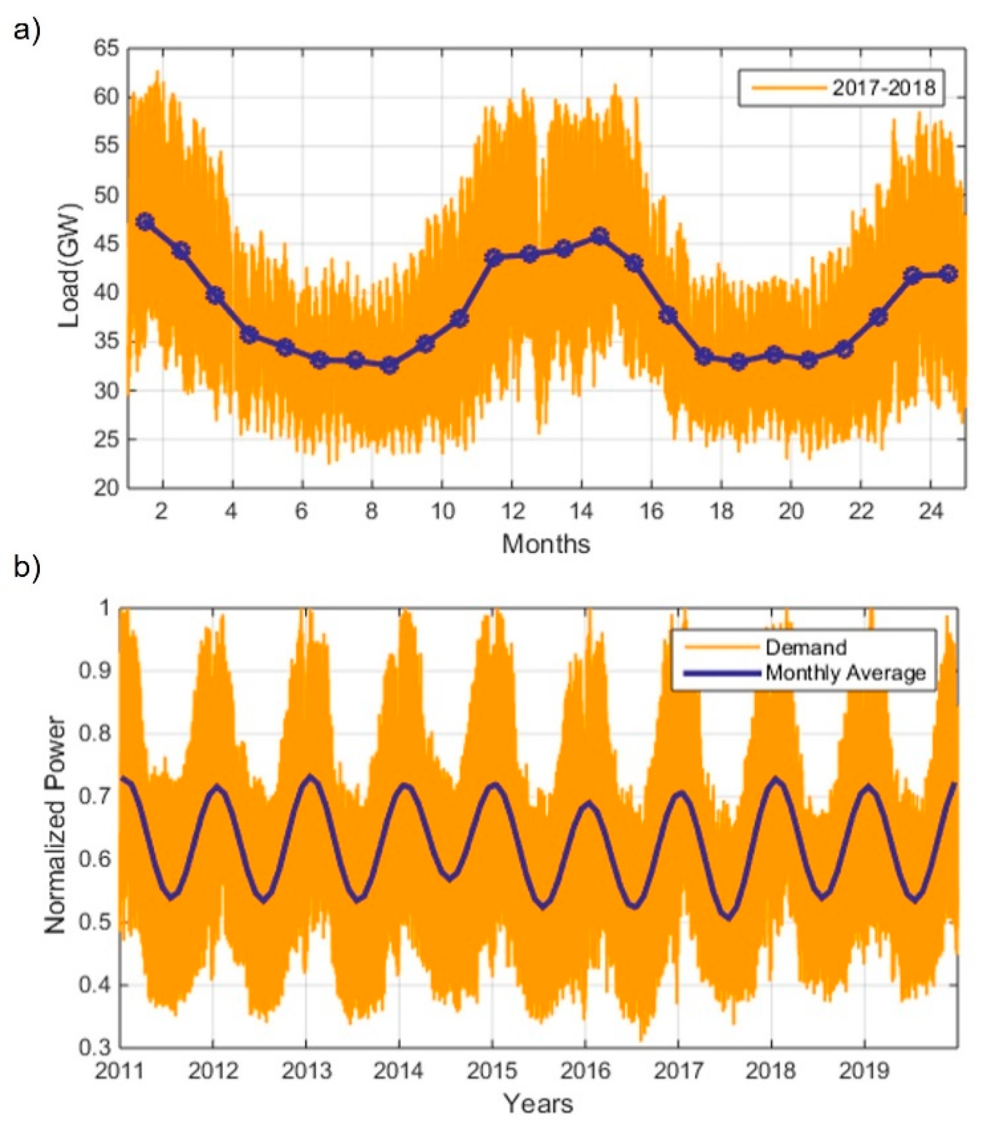
Figure 1a shows the profile of electricity demand in the UK in 2017 and 2018 [25]. In 2018, the country consumed approximately 335 TWh of electricity [26]. The maximum power seen by the grid at any one time is ~60 GW.
Figure 1b shows the profile of historical electricity demand in the UK from 2011 to 2019 [25,27]. This profile is used as one of the inputs for the model. The data shown in the figure have been normalized on an annual basis to facilitate their use. Details on the way the data are handled are discussed in Section 3.
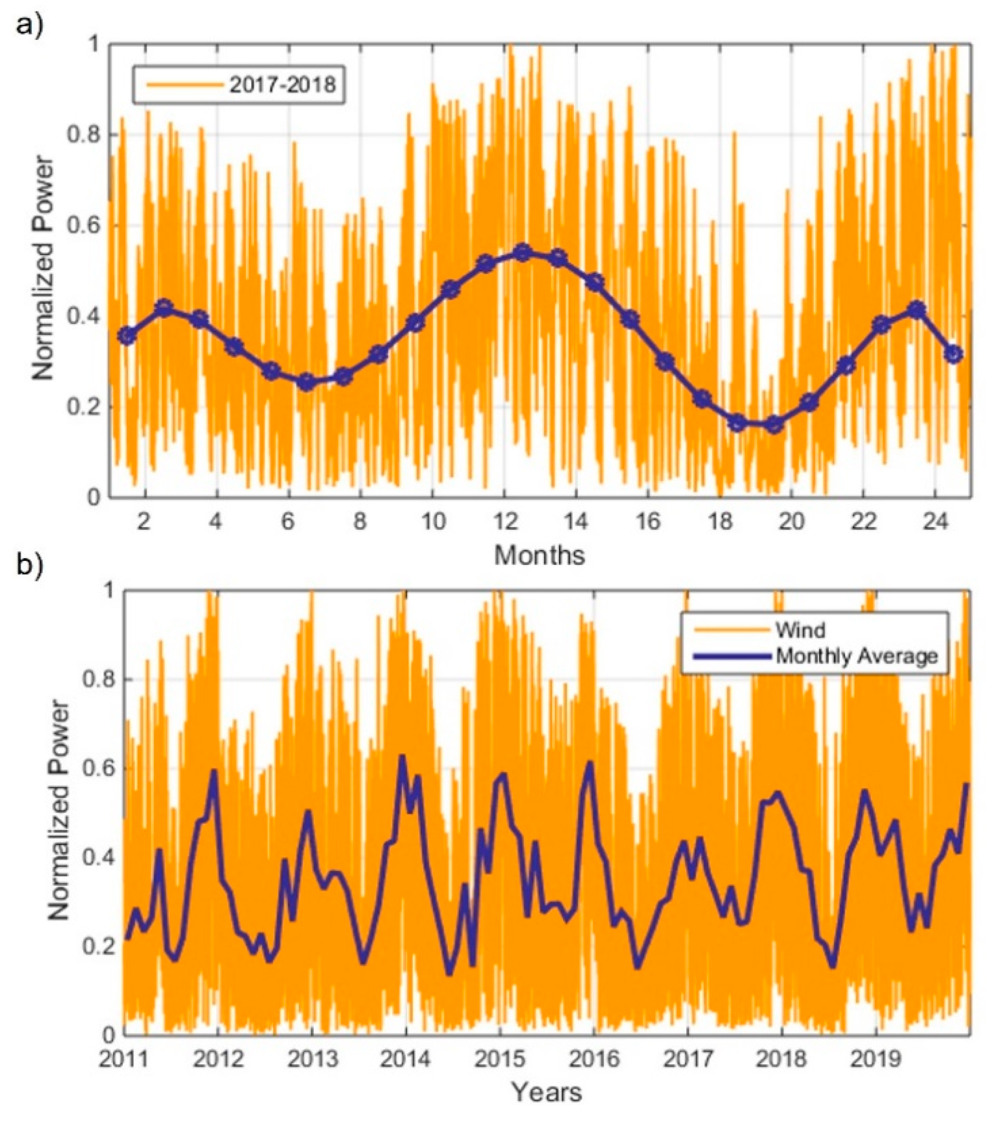
Figure 2 shows the profile of wind power generation in the UK in the period 2017–2018 [25,27]. We can see that there are marked diurnal, day-to-day, and seasonal variations [28]. In 2018, approximately two-thirds of the total wind output was produced during the colder months (October–March) [29]. Figure 2b shows the profile of wind power generation from 2011 to 2019 [25,27]. The normalized data account for the increase in installed capacity. The strong inter-annual variability of wind output can easily be seen here.
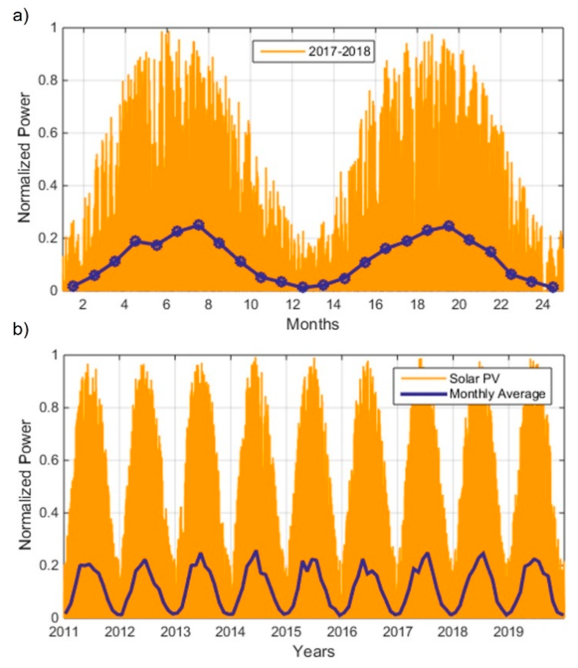
Figure 3a shows the profile of solar-PV power generation in the UK in the period 2017–2018 [30]. The inter-day variations in the solar resource are considerably smaller than in the case of wind power. However, solar-PV power generation in the UK has a stronger seasonality. Approximately 75% of all the electricity generated by PV panels in 2018 was produced between April and September [28].
Figure 3b shows of the profile of solar-PV generation data over the 9 year period [31]. This normalized profile shows the estimated power output of a 1 KW (rated) solar panel based on UK historical (measured) solar irradiation data.
Analyzing a single year of data has the risk of missing some of the potentially large inter-annual variations in renewable generation, which can lead to a severe underestimation of how much energy storage capacity is needed [32]. The actual storage capacity that is required to deal with the inter-annual variability of renewables is several times larger than what a single-year analysis may suggest.
3. Methodology
In a previous study, Cardenas et al. quantified the energy storage capacity that the UK will need to achieve a renewable penetration of 100% by 2035 [24]. Different mixes between wind and solar-PV power as well as different levels of over-generation were explored. It was found that for a renewable penetration of 100% and ~43 TWh of storage capacity are needed. This result considers a mix of 85% wind + 15% solar-PV, a storage efficiency of 70% and over-generation of 15% of the total electricity demand. The mix of renewables has a strong effect on the storage capacity required. Depending on the mix, the profile of generation may resemble to a greater or lesser extent the profile of demand. For example, a 100% wind-based supply would require ~74 TWh of storage whilst a 50% wind + 50% solar would require ~68 TWh. It was found that a mix of 85–15% is the optimum, requiring only ~43 TWh with a storage efficiency of 70%. A lower storage efficiency leads to a greater storage capacity requirement.
This paper assumes an 85/15% wind + solar-PV mix. Nuclear power is not considered in the mix because it is too expensive to achieve a significant uptake as the UK decarbonizes its generation fleet. Wind power has already achieved costs per MWh that are less than half of what nuclear can offer [33]. The costs of wind and solar-PV keep reducing at an accelerated pace. For this reason, the authors believe that nuclear will not play a significant role in the UK.
This paper explores mixes of different storage technologies (hydrogen, compressed air, and lithium ion) to find the most economical way of supplying the storage capacity that a 100% renewable-based electricity grid needs.
Hydrogen is excellent for long-duration (or bulk) energy storage as it is very cheap, but it is not ideal for frequent charging/discharging due to its low efficiency. Conversely, batteries are ideal for fast transactions but are not well suited for holding large amounts of energy due to their high cost per unit capacity. CAES bridges the gap between these two technologies, being an excellent alternative for medium-duration storage [34,35].
This study is divided into two phases. The first phase uses demand and generation data with a resolution of 1 h to determine the optimum split (from an economic standpoint) of the total energy storage capacity between H2 and CAES. The second phase focuses on the optimum H2/CAES mix found and uses data with a much finer resolution of 5 min to determine the duty of Li-ion batteries.
Batteries have a considerably higher cost per unit storage capacity than H2 and CAES systems. Therefore, their total installed capacity will be small compared to the other two technologies. Notwithstanding, they are key to dealing with short-duration imbalances in the grid as H2 and CAES not only have lower efficiencies but also have slower response times and ramping capabilities which impede them from reacting to fast changes in frequency in the grid [36].
The reason for having two datasets is pragmatic, as carrying out all the analyses using 9 years of data with a 5 min resolution (~1 million points per time series) is too computationally demanding for it to be feasible.
3.1. Splitting Net Demand into Work Cycles for Long- and Medium-Duration Stores
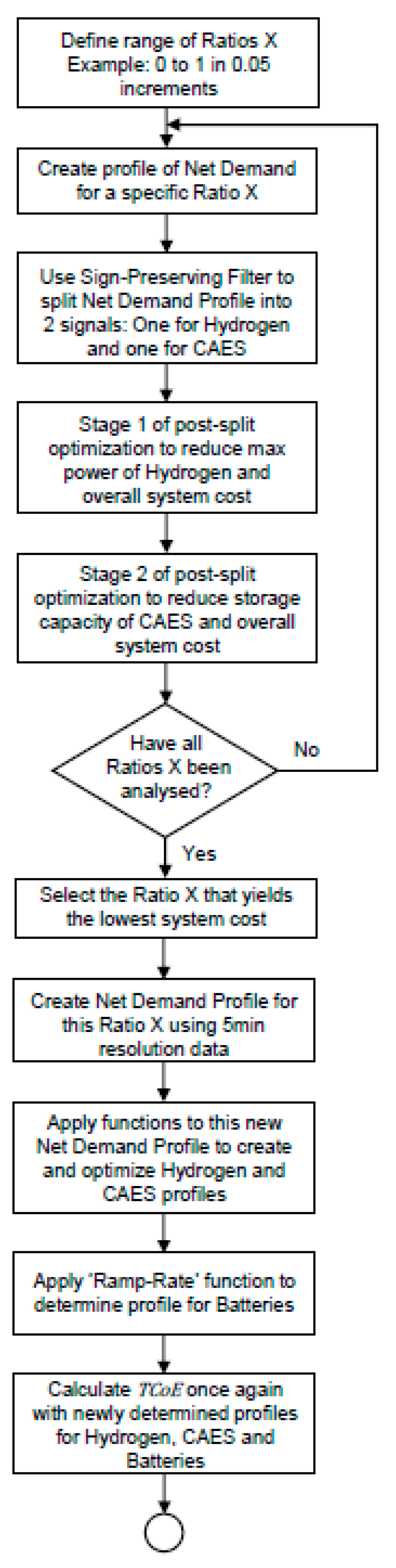
Figure 4 shows the general process followed. The split of the storage duty between H2 and CAES is characterized by a ratio called X. This ratio indicates the proportion of the energy that is put into CAES with respect to the total energy that will be put into storage. The fraction of the storage duty that is provided by H2 is the remainder (i.e., 1 − X). A ratio X = 0 indicates that hydrogen is providing all the storage capacity while a ratio X = 1 indicates that CAES provides all the storage capacity.
A one-dimensional analysis is carried out by varying X. For each value of X, a profile of net demand is created. Net demand refers to the difference between electricity demand and renewable generation. The periods when net demand is negative are times when electricity should be stored. The periods when net demand is positive are times in which the electricity stored is discharged to meet demand.
Determining the profile of net demand is an iterative calculation. The process starts by estimating how much renewable energy is needed (). This is done by means of Equation (1), where is the total energy demand over the period analyzed, Ω is the percentage of allowable over-generation and L are the total storage losses. The first guess for L takes a value of zero.
The normalized profiles of wind and solar generation are amplified so that the energy that each resource produces over the 9 year period corresponds to its penetration level (85% for wind, 15% for solar). The profile of net demand () is created by subtracting the amplified wind and solar profiles from the profile of electricity demand ().
The next step is to integrate to determine the energy content below zero () and above zero (). includes the energy that will be put into storage as well as the energy that will be curtailed. is the energy that the store will return to the grid.
The energy that comes out of the store should be equal to the energy that went into the store multiplied by the storage efficiency. The combined efficiency () of the two types of energy stores is used.
A check variable is calculated as Equation (3) shows. The iterative process concludes when ‘check’ equals the combined efficiency of the two stores. The amount of renewable generation required to meet demand and to compensate for storage losses has been calculated and the profile of net demand is now known.
The profile of net demand will change as the value of X varies, because H2 and CAES have different efficiencies. As X becomes smaller, more energy is put into the H2 store, which represents increased losses. The output of renewables is amped up to compensate for the increased losses and this changes the shape of the net-demand profile.
Before proceeding to split the net-demand profile into two separate work cycles (for H2 and CAES), it is necessary to remove the energy that was over-generated. This is still embedded in the negative part of the profile.
To avoid prescribing the times where curtailment occurs, a time-stepping algorithm is adopted [24]. The process begins by making a guess for the capacity (‘size’) of a single store. The algorithm models the operation of the store throughout the work cycle. If the energy store is too small, there will be excessive curtailment of energy. The guess for the storage capacity is updated and a new iteration is carried out. The process concludes when at the end of the work cycle, only the correct amount of energy has been curtailed. Curtailment has occurred where it was necessary rather than at prescribed times. Three important things are revealed: (1) the minimum storage capacity (provided by a single store) required to handle the duty, (2) the profile of curtailment and (3) the profile of net demand without any ‘excess’ energy.
Determining the optimum amount of over-generation is a decision based on economics. Small percentages of over-generation lead to a reduction in the cost of the energy store. These savings exceed the increase in the cost of generation. It has been found that the optimum level of over-generation for the UK is ~15% [24]. However, this figure depends on the storage efficiency considered. In this study, the overall efficiency varies with X.
A parallel analysis was carried out to determine the optimum level of over-generation (Ω) for each ratio X. For values of X close to 1 the optimum, Ω is ~17% of total demand, while for values of X close to 0, the optimum Ω is ~7%. This is discussed in further detail in Section 4.1. The values found are used to produce the different net-demand profiles for the different values of X.
Figure 5 shows some of the different net-demand profiles created. In the figure, we can see the portion of over-generated energy that has been removed.
After having curtailed the over-generated energy from the profile of net demand, we can proceed to create the work profiles for the H2 and CAES stores. This is done by splitting the profile of net demand into two separate profiles using a ‘sign-preserving filter’. This filter will be used as the primary tool for creating the work cycles for the different system configurations explored. A comprehensive explanation of the mechanics of the filter’s operation can be found in [37].
The filter takes a curtailed profile of net demand (A) and splits it into two work cycles, a mostly low-frequency one (B) which is assigned to H2 and a mostly high-frequency one (C) which is assigned to CAES. The key feature of the filter is that both work cycles created always have the same sign. This prevents energy counter-flow (i.e., discharging one store to charge the other), which is undesirable due to the stack up of inefficiencies.
The signal splitting or ‘filtering’ is an iterative process. The process stops when the energy content of C (profile for CAES) corresponds to the value defined for X. As mentioned, the proportion of energy that the hydrogen store will receive is 1 − X. After the splitting the net-demand profile, the energy content of signal (profile for H2) corresponds to the value of 1 − X.
Figure 6 shows the different splits created for different ratios X. This is the result of passing the net-demand profiles through the sign-preserving filter. For simplicity, not all ‘splits’ are shown.
3.2. Post-Split Optimization of the Work Cycles
The two profiles produced by the filter for any given ratio X (shown in Figure 6) could be used directly as inputs for the techno-economic assessment. However, each pair or ‘split’ can be optimized to achieve a lower overall system cost. This post-split optimization is done in two stages. The first stage focuses on flattening hydrogen’s charging/discharging power, as it has a higher cost per kW than CAES. The second stage focuses on reducing CAES’ storage capacity (without reducing the energy that passes through it) as it is more expensive per kWh than H2.
For the first stage, we make use of a simple script which identifies the maximum charging power in the hydrogen profile (negative side) and creates a cut-off line at a given Δ from it. The function identifies all the negative points in the H2 profile below the cut-off line. All these points are removed from the H2 profile and added to the CAES profile.
In order to keep the ratio X constant, the function needs to carry out the inverse operation (compensation) as well. It finds others points in the profiles where power can be added to the H2 profile and removed from CAES. Choosing where to perform the compensation requires evaluating the overall cost of the system to ensure that the overall system cost is indeed reducing.
The function keeps moving the cut-off line by Δ until no further reallocation of points is possible. Then, a similar process is carried out for the positive part of the H2 profile, which represents the discharge power of the store.
The second stage of the post-split optimization focuses on reducing the storage capacity of CAES. The storage capacity of both energy stores can be calculated by integrating the work cycles and looking at the curve of accumulated energy over time. The storage capacity required is given by the difference between the maximum and minimum values of the curve of accumulated energy.
A script like the one used in the first stage of post-split optimization is launched. This function focuses first on the positive side of the profiles. It reduces the discharge power of CAES at a given time t by an amount Δ and increases the discharge power of H2 at that same time t by the same Δ. The function needs to carry out a balancing operation somewhere else in the profiles to keep the ratio X constant.
The objective of these rearrangements is to reduce the difference between the maximum and minimum values of the CAES’ profile of accumulated energy, which directly reduces the storage capacity of CAES. The capacity of H2 will increase because of this re-arrangement.
Several iterations are carried out with a decreasing Δ. The iterations end when there are no more points whose reallocation yields a reduction in the storage capacity of CAES and the overall system cost. A similar procedure is carried out with the negative side of the profiles. Figure 7 shows a comparison of the work profiles for CAES and hydrogen (for X = 0.5) after the sign-preserving filter and after the post-split optimization.
Figure 8 shows the work profiles created for different splits after having been processed through the two stages of post-signal optimization. This concludes the first phase of this study, which uses data with a resolution of 1 h to determine the optimum split of the storage duty between H2 and CAES. With the profiles shown in Figure 8, an economic assessment is carried out to find which split leads to the lowest overall system cost. Section 4.1 provides a discussion on this preliminary techno-economic assessment.
The second phase of this study takes the H2/CAES split that yields the lowest system cost and repeats all the calculations for this specific ratio X using data with a resolution of 5 min. After the profiles have been optimized, an additional ‘ramp-rate’ function is used to determine the duty of Li-ion batteries, which will be the high-frequency (short-duration) energy store of the system. Section 4.2 discussed in detail the ramp-rate function as well as the economics seen after the introduction of batteries to the storage mix.
4. Results and Discussion
4.1. Preliminary Assessment Based on Hourly Data
Using the splits of net demand shown in Figure 8, this section analyzes how different system parameters vary with respect to the mix of storage technologies. An economic assessment is carried out to determine the value of X that yields the lowest possible total cost of electricity (TCoE).
This study assumes that renewables supply 100% of the country’s electricity, which could happen as early as 2035. A mix of 85% wind + 15% solar-PV is considered. This generation mix was determined to be optimal for the UK in a previous study by Cardenas et al. [24]. Different proportions of wind and solar will cause a greater mismatch between the profiles of generation and demand, which leads to an increased energy storage capacity requirement.
This study does not consider nuclear as it is too expensive in comparison to renewables in the UK. Nuclear has a cost of ~92 £/MWh [38] while wind and solar-PV power have already achieved costs as low as 40 £/MWh [39,40] and 60 £/MWh [41,42], respectively. The cost of renewables is reducing at a fast rate and is unlikely that nuclear will achieve similar cost reductions. For this reason, we think the contribution of nuclear to the UK’s energy mix in a 2035 or even a 2050 scenario will be minimal.
The analysis presented in this paper is based on current demand levels. Forecasting what the electricity consumption will be in the coming years is an important but broad area of research, which is out of the scope of this study. Nevertheless, the results of this work will provide valuable information.
Electricity demand is expected to increase with time as the population and economy of the country grows. The installed renewable capacity will also increase with time to follow demand and to meet decarbonization targets. After we achieve a renewable penetration of 100%, an increase in demand will prompt a proportional increase in renewable generation. What determines the energy storage capacity needed is not so much the magnitude of demand or generation, but the penetration of renewables and how closely the profile renewable generation matches that of electricity demand.
Electric vehicle (EV) charging is an interesting future load to consider. Currently their uptake is small, but it will grow rapidly in the coming years. We do not know with certainty what the charging patterns will be. However, a reasonable assumption is that EV charging will have very well-defined daily patterns and little seasonality: people return from work at the same time every day and they need to drive throughout the year. This means a proportional increase in the demand profile across the whole year. Renewable generation will also increase in order to supply the additional demand. This proportional increase in both quantities (demand and generation) may not affect dramatically the requirement for energy storage. As mentioned before, the amount of storage capacity required depends much more on the shape of the profiles and how well they match each other, rather than on their absolute magnitudes.
The storage capacity requirements presented in this paper can be seen as an assessment or estimation of the energy storage capacity that the country will need to decarbonize its electricity grid by 2035 if the future pattern (not magnitude) of consumption resembles the current pattern, and if the pattern of renewable generation resembles the behavior of the resources over the past 9 years.
In this study, regardless of the distribution of storage capacity between the two technologies (CAES and H2), renewables generate a ‘baseload’ of 3015 TWh over the 9 year period analyzed. An average annual demand of 335 TWh (similar to current level) is considered, but there are year-to-year differences in generation. Considering the aforementioned wind + solar mix, these inter-annual differences can be +11% or −16% with respect to the average value.
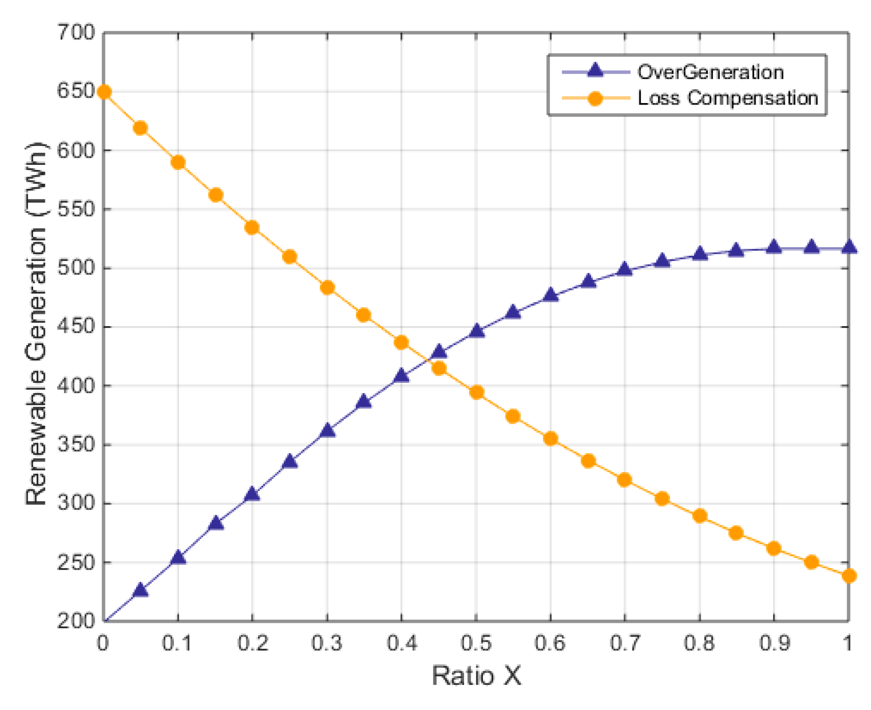
In addition to the baseload, there are two other components of renewable generation that do vary with respect to X; these are shown in Figure 9. The first component of additional generation relates to the storage losses. The amount of energy generated is calculated so that after losses there still is enough energy in the system to meet net demand. CAES has a higher efficiency than H2 storage; therefore, as X increases, the overall system losses reduce.
When all the storage capacity is provided by hydrogen (X = 0), the system sees losses of approximately 650 TWh, which is equivalent to ~21% of the total demand. On the other hand, when the storage capacity in the system is provided entirely by CAES, energy losses reduce to ~8% of the total demand.
The other component of variable renewable generation is ‘over-generation’, which is a small amount of additional generation calculated as a percentage () of the total demand. In this work, over-generation is independent of the extra-generation required to compensate for storage losses. Some over-generation in the system improves the match between the generation and demand profiles, which reduces the requirement for energy storage capacity. The ‘loss compensation’ generation has this effect too albeit to a lesser extent.
Figure 9 shows that greater values of X allow larger amounts of over-generation. This is because smaller X ratios require larger amounts of energy to compensate for storage losses, which leaves little room for any further extra generation. Generation costs start to counteract the economic benefits of a reduced storage capacity.
A preliminary assessment was carried out to determine the optimum level of over-generation for each one of the different values of X. This assessment used the economic figures shown further on in Table 1. The preliminary assessment explored several values of Ω for each specific ratio X. A profile of net demand was created for each combination of Ω and X. This net demand profile was split into two components using the sign-preserving filter and a TCoE was calculated. The optimum Ω for a given X is the one that minimizes TCoE. The blue curve in Figure 9 shows the optimum level of over-generation for each ratio X.
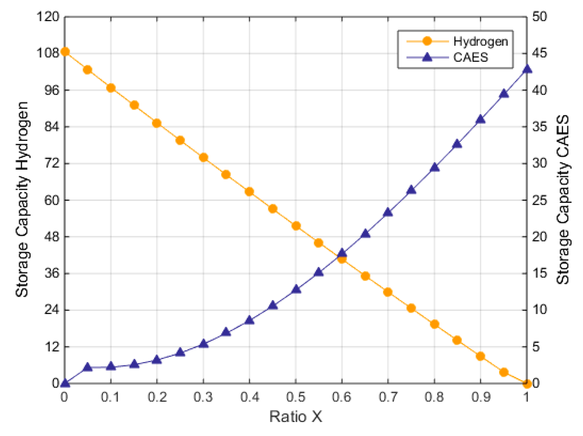
Figure 10 shows how the storage capacity varies with respect to X. The storage capacities shown in the figure are calculated based on the optimized profiles shown previously in Figure 8. In an X = 0 scenario, ~108 TWh of capacity in the form of H2 is needed. On the other hand, an X = 1 scenario requires ~42 TWh of CAES storage capacity, which is similar to previous findings in [24].
The considerable difference in capacities between the two ends of the X range is caused by the different efficiencies of the two storage technologies. H2 storage has a roundtrip efficiency of ~45% [43] (~80% electrolyzer and ~55% turbine [44]) whilst CAES can achieve a much higher efficiency of ~70% [9,10]. Consequently, for a given energy output, H2 will need a greater energy input and larger storage capacity than CAES.
This study treats the UK’s electricity grid as a single node and determines the amount of storage capacity required to balance the system. In this study, this storage capacity is provided by 2 large, centralized stores (H2 and CAES). In reality, the total storage capacity will be provided by an array of small energy stores distributed throughout the country.
The location of these stores is important to prevent grid congestion and avoid excessive transmission losses. Research effort should be devoted to understanding this, but it is out of scope for this paper. A reasonable assumption is that the small stores could be located next to generation sites. In any case, the location of the stores does not have a big effect on the amount or type of storage capacity that is required, which is the focus of this paper.
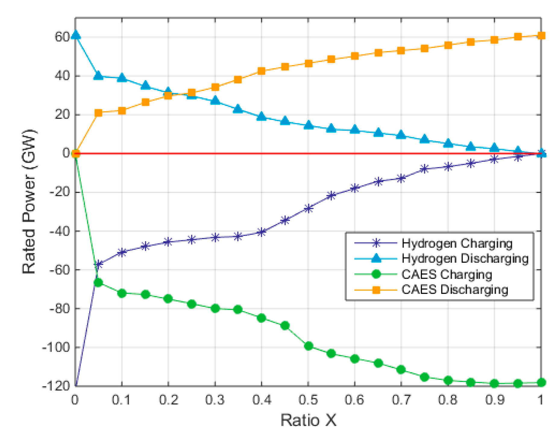
The rated powers of the two stores are another important set of parameters. H2 storage uses markedly different technologies for converting electricity into hydrogen (electrolysis) during the charging phase and for converting hydrogen back to electricity (combustion in turbines) during the discharge phase [45,46]. These two very different technologies have very different costs per unit power. Large-scale CAES also uses different sets of machinery for charging (compressors) and discharging (expanders) the system. The compression and expansion processes are similar to each other therefore the two sets of machinery have similar costs.
Figure 11 shows how the rated charging () and discharging () powers of H2 and CAES vary with respect to X. As expected, the charging and discharging powers of CAES increase with X whilst the rated charging and discharging powers of hydrogen increase as X reduces. The maximum rated discharge power of either store is ~60 GW as this is limited by the demand profile (See Figure 1).
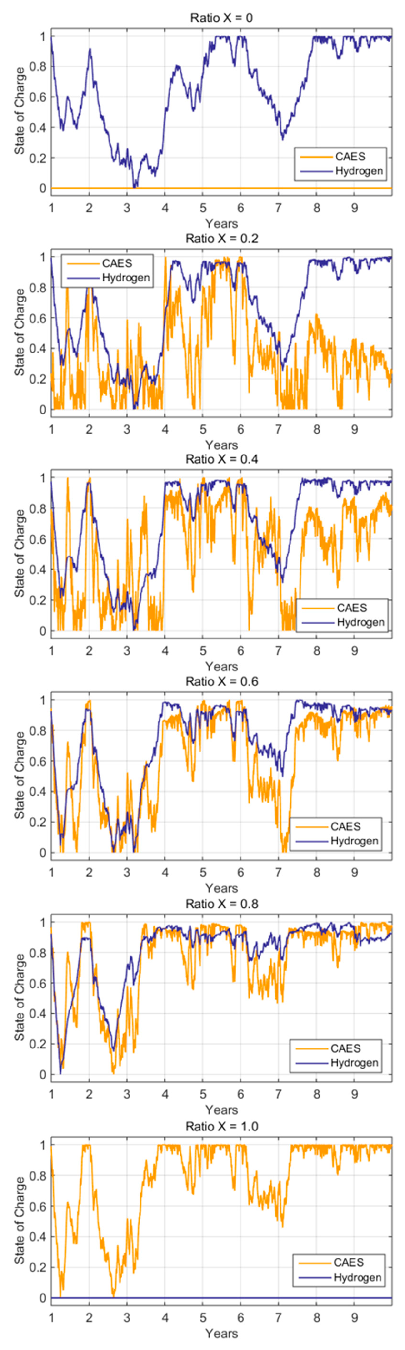
Figure 12 shows the evolution of the state of charge (SoC) of the two stores throughout the 9 year period analyzed. Regardless how net demand is split, the work profiles of the two stores are balanced. The energy that is put into a store throughout its work cycle is equal to the energy that comes out of that store (useful output + losses). Because of this, the stores start and finish their operation with the same SoC.
Figure 12 reveals an interesting aspect of the system’s operation. The state of charge of the H2 store moves at a much slower rate than that of CAES. Regardless of X, the hydrogen store becomes fully charged (SoC = 1) or discharged (SoC = 0) much less frequently than CAES. This is owed to the fact that the low-frequency component produced by the sign-preserving filter was assigned to hydrogen, while CAES was given the high-frequency profile.
As shown in the graphs, the low-frequency work cycle (assigned to H2) deals with the inter-annual variations in renewables. In this case, hydrogen helps shifting ‘excess’ energy from some years into other years in which renewable generation is not enough to meet demand. This task requires very large storage capacities. H2 storage is very well suited for this role due to its very low cost per kWh [36].
On the other hand, the high-frequency work profile (assigned to CAES) deals with the day-to-day and seasonal variations in renewables. This task requires much smaller storage capacities compared to inter-annual energy shifting. The work profile for CAES becomes a medium-frequency profile after batteries are added to the storage mix. Batteries take on the high-frequency (short-duration) energy storage duty.
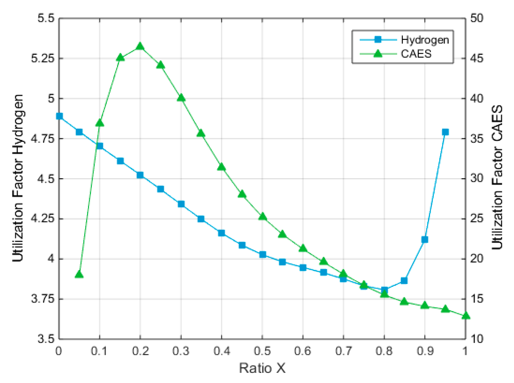
As shown in the graphs, CAES has a faster charging/discharging rate than H2, therefore its storage capacity is much better utilized. The storage capacity of CAES is ‘exercised’ more due to how much more energy passes through it with respect to its capacity. A utilization factor can be defined as the ratio between the energy output of a store with respect to its storage capacity.
Figure 13 shows how the utilization factor of both stores varies with respect to the ratio X. The utilization factor of hydrogen (left axis) takes values between 3.8 and 4.8 depending on the value of X. This reinforces what was seen in the state-of-charge plots; the H2 store accumulates large amounts of energy but it does not discharge often. The storage capacity is mostly used to shift energy to years with low renewable generation.
In contrast, the utilization factor of the CAES store (right axis) goes from 12.8 up to 46.5 depending on the value of X. At a ratio X = 0.5, the utilization factor of CAES is 25.2 while the utilization of H2 is only 4. The large utilization factors of CAES are owed to the frequency of its work cycles (i.e., how often the store is charged and discharged). A high-frequency profile allows a greater amount of energy to pass through storage in a given period of time.
The remainder of Section 4.1 focuses on the economics of the energy stores and the overall electricity system. The capital cost of either store () can be calculated by means of Equation (6). In the equation, α is the cost per unit of storage capacity (£/kWh) of the particular technology, β is the cost per unit power of the charging machinery (£/kW) and γ is the cost per unit power of the discharging equipment (£/kW).
In a CAES system, the storage capacity cost is linked to the provision for storing air at a high pressure, which for systems of relevant size is normally an underground solution-mined cavern [47]. The power costs are related to the compression/expansion machinery used to charge and discharge the system. According to figures available in the literature, the cost per unit capacity (α) of a CAES system is ~3.5 £/kWh and the costs per unit rated power β and γ are ~300 £/kW [48,49].
In a power-to-H2 storage system, the cost of storage capacity relates to the ability to store hydrogen. Similar to compressed air, hydrogen can also be stored in underground caverns [50,51]. According to some figures available in the literature, the cost per unit capacity of hydrogen storage is ~0.67 £/kWh [52]. This cost is lower than that of CAES because the volumetric energy density of hydrogen is higher in comparison to compressed air.
Electrolyzers are used during the charging phase to produce H2. Electrolyzers currently have costs of ~1100 £/kW [53]. There are two options for discharging the energy stored: (i) fuel-cells and (ii) burning hydrogen and using turbines to produce mechanical work. Fuel cells can achieve higher efficiencies than turbines but their costs would be too expensive for large-scale applications. Turbines have costs in the order of ~450 £/kW [54,55].
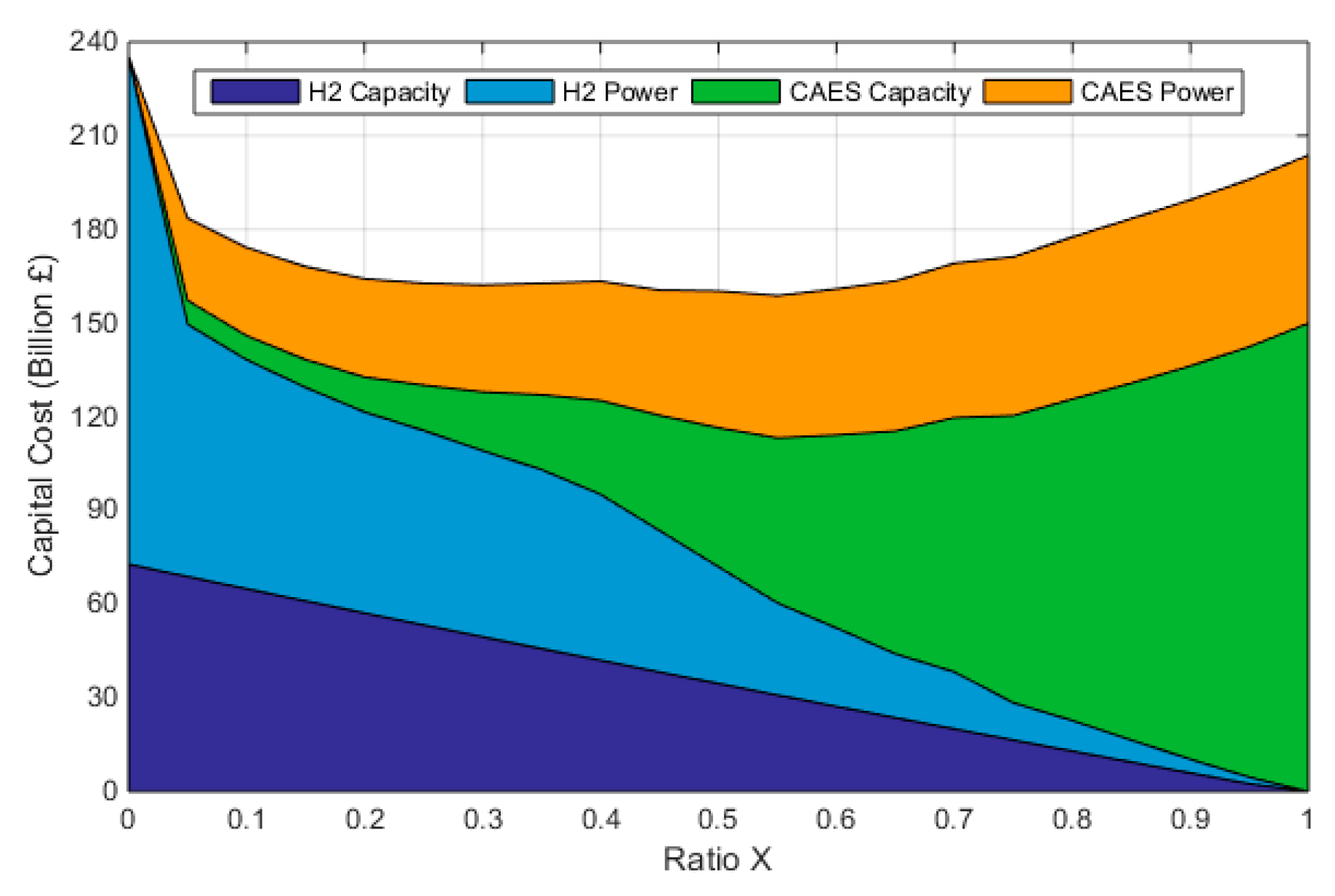
Figure 14 shows how the overall capital cost required for the energy stores varies with respect to X. The figure breaks down the total capex into storage capacity costs and power conversion costs. When all the storage capacity is provided by hydrogen, the capital cost adds to ~£235 bn. In this system configuration, the hydrogen storage capacity represents 31% of the cost while the power conversion machinery accounts for the other 69%. More than 80% of the power conversion cost is owed to the electrolyzers used for ‘charging’ the stores.
On the other hand, when CAES provides all the storage capacity for the system, the capital cost required reduces to ~£204 bn. In this configuration, 74% of the cost is owed to the storage capacity while the power conversion machinery (compressors/expanders) account for the remaining 26%.
The capital cost is minimized in the region 0.45 ≤ X ≤ 0.55. For a ratio X = 0.5, the total capex is £160.25 bn. CAES accounts for 55% of this cost while H2 makes up the other 45%.
The costs shown in Figure 14 represent the capital expenditure associated with the energy storage provision (capacity + power) required to support a 100% renewable electricity grid. These costs do not consider the cost of the generation capacity. The ‘total cost of electricity’ () or ‘total system cost’ is a metric that includes the two main contributors of cost: the capex of the energy stores and the cost of generating electricity. The represents the total average cost of producing and storing a unit of electricity. In this study, the transmission and distribution costs are not included in the calculation.
The cost of generating electricity is given by the levelized costs of wind and solar-PV. The levelized cost of electricity () is a lifetime cost that encompasses capital cost, load factors, efficiencies, operation costs, and other expenses associated with the generation of electricity. This paper uses economic figures available in the literature (provided in Table 1). The system’s is calculated through Equation (7):
In Equation (7), is the total electricity demand over the 9 year period (3015 TWh). is the total energy generated by renewables and comprises baseload generation, loss compensation, and over-generation. The penetrations of wind and solar ( and ) are 85% and 15%, respectively. is the total cost of the energy generated from wind while is the cost of the energy produced by solar panels.
The calculation of the TCoE considers a fraction of the capex of the stores that is proportional to the 9 year period (τ) that is being analyzed. A useful life (λ) of 30 years is assumed for both CAES and H2 [36,56,57].
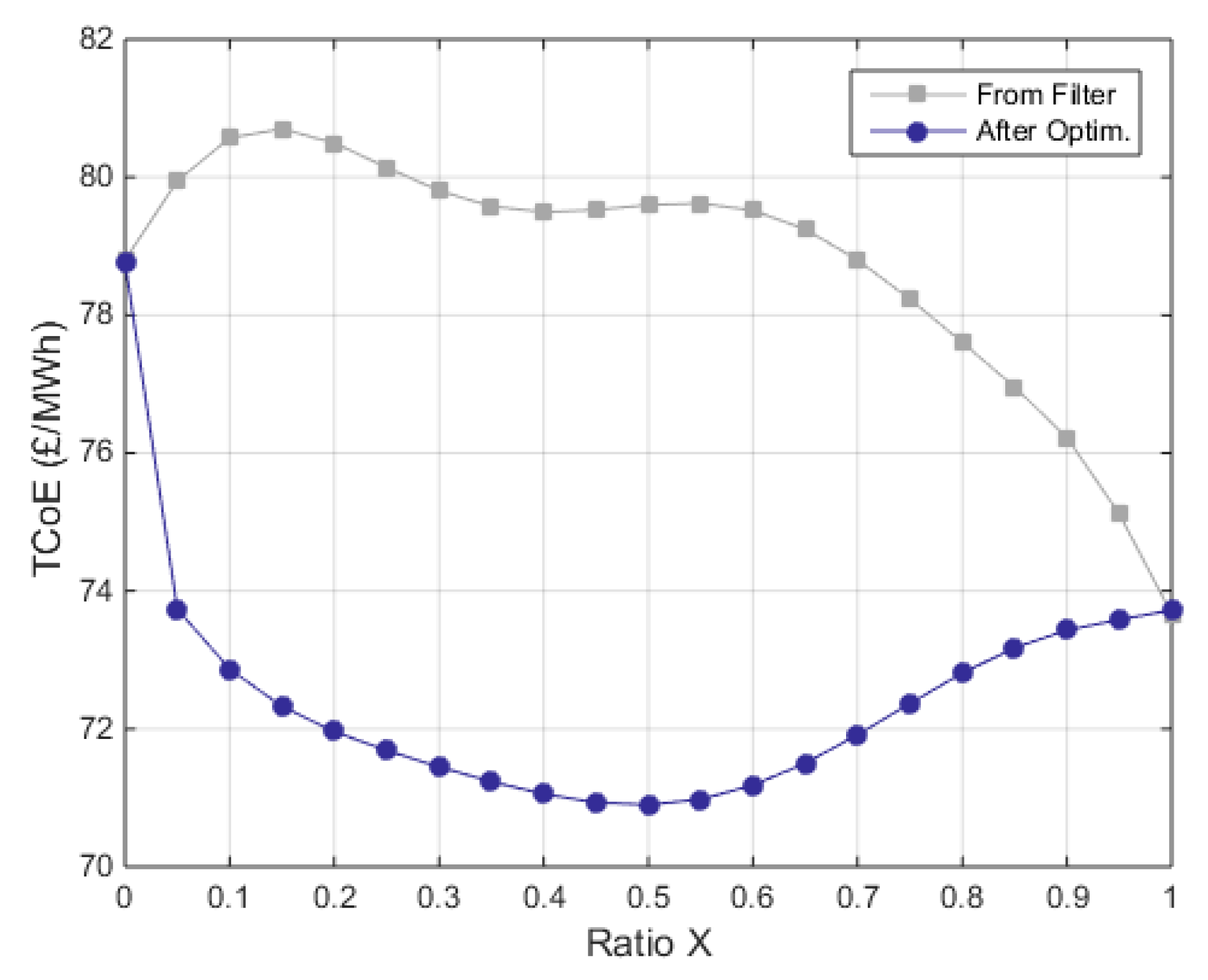
Figure 15 shows the total cost of electricity (generation + storage) for different values of X. Table 1 summarizes the economic figures used for the calculation. The figure shows 2 curves: grey and blue. The grey curve shows the costs calculated with basis on the profiles obtained from the filter (pre-optimization). Given that those profiles had not been optimized in any way, their costs are high.

Table 1.
Figures used for the calculation of the total cost of electricity.
| Value | Unit | Ref. | |
|---|---|---|---|
| LCOE of wind | 40 | £/MWh | [39,40] |
| LCOE of solar PV | 60 | £/MWh | [41,42] |
| CAES storage capacity cost (α) | 3.5 | £/kWh | [48,49] |
| CAES charging power cost (β) | 300 | £/kW | [48,49] |
| CAES discharge power cost (γ) | 300 | £/kW | [48,49] |
| H2 storage capacity cost (α) | 0.67 | £/kWh | [52] |
| H2 charging power cost (β) | 1100 | £/kW | [53] |
| H2 discharge power cost (γ) | 450 | £/kW | [54,55] |
| Lifetime of CAES (λ) | 30 | Years | [56,57] |
| Lifetime of H2 (λ) | 30 | Years | [36,57] |
It can be seen in the figure that a system that only uses CAES would achieve a TCoE of 73.7£/MWh, which is considerably lower than the 78.8 £/MWh that would be seen if all the storage capacity were provided by hydrogen.
The blue curve (post-split optimization) reveals that the system cost is minimized with X = 0.5. For clarity, a ratio X = 0.5 indicates that both stores (H2 and CAES) receive the same amount of energy throughout the 9 year period. However, their outputs are not the same due to their different efficiencies. Table 2 summarizes the technical parameters of the system configuration based on a ratio X = 0.5, which achieves the lowest TCoE.
At the optimum ratio X = 0.5, the system sees a TCoE of 70.9 £/MWh. A reduction of ~4% with respect to the cost that could be attained with X = 1 may seem small at a first glance. However, considering an annual demand of 335 TWh, this reduction in the TCoE translates into yearly savings of up to ~£938 million.
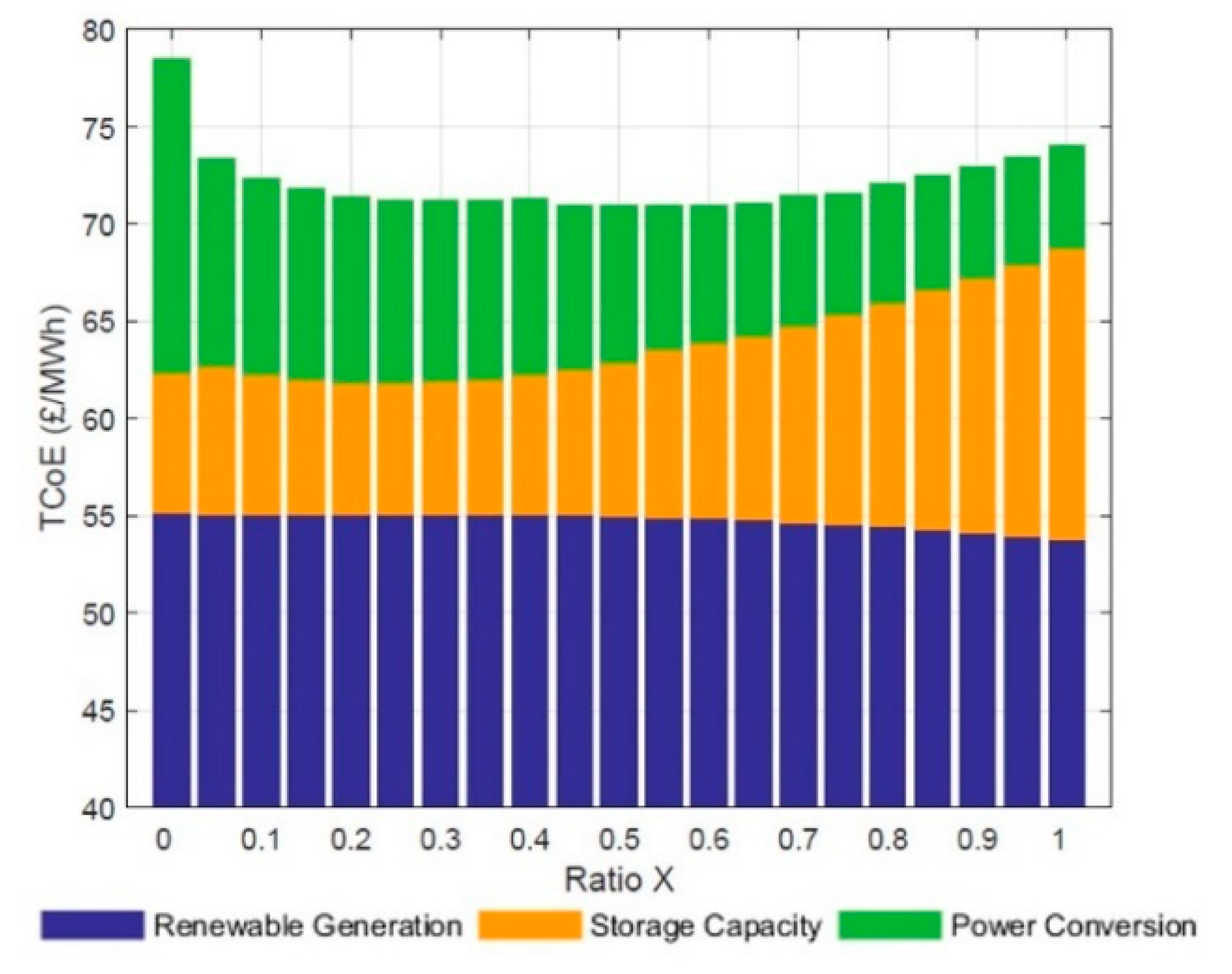
Figure 16 presents a simple decomposition of the TCoE for different values of X into three cost components: generation, storage capacity and power conversion equipment. Regardless of the value of X, generation accounts for more than 70% of the TCoE. Depending on X, storage capacity accounts for between 9% and 20% of the TCoE. The contribution of storage capacity to the overall system cost increases with X as CAES has a higher cost per kWh of storage capacity.
The cost of the power conversion machinery displays almost the opposite effect. The cost of power conversion reduces as X increases since CAES charging/discharging machinery is cheaper per kW than the equipment used to transform electricity into hydrogen and back into electricity. Power conversion costs account for between 7% and 21% of the total cost of electricity.
Figure 17 presents a sensitivity analysis of how the varies with respect to the cost of the two energy storage technologies. In all three figures, we see the same blue line that was shown in Figure 15. This line is the calculated with the values given in Table 1.
Figure 17a shows the effect that a change in the cost per unit storage capacity (£/kWh) of either technology has on the . Four cases are shown: a 25% increase and a 25% reduction in the storage cost of H2 and CAES. In each case, only 1 cost varies whilst every other cost stays constant. Figure 17b shows the effect of an increase and a reduction in the cost of power conversion of hydrogen. It should be noted that the increase/decrease applies to both sets of machinery (charging and discharging). Lastly, Figure 17c shows the effect that a +/−25% variation in the power conversion of CAES has on the seen by the grid.
For the optimum system configuration (X = 0.5), Table 3 provides a summary of the individual contributions of different system components to the TCoE. In this optimum scenario, 3855 TWh of electricity are generated over the course of 9 years. This amount encompasses a baseload of 3015 TWh to meet demand, 394 TWh to compensate for storage losses and 446 TWh of over-generation (Ω~15%), which are curtailed. A total of 85% of the total electricity produced comes from wind power, while solar-PV panels generate the other 15%.
Baseload generation accounts for 60.7% of the total electricity cost, while loss compensation and over-generation contribute 7.9% and 8.9% to the TCoE, respectively.
This configuration requires an overall storage capacity of 64.3 TWh. Hydrogen provides ~80% of the total storage capacity, which represents 4.9% of the TCoE. CAES contributes a much smaller capacity of 12.7 TWh to the system. However, it accounts for 6.3% of the TCoE.
Throughout the 9 years there are 927 TWh of electricity that need to be put into storage. As the ratio X = 0.5 indicates, each store receives exactly 50% of that. Having an efficiency of 70%, CAES loses 139 TWh whilst hydrogen, due its lower roundtrip efficiency loses ~255 TWh.
CAES has a rated charging power of −99.3 GW and a rated discharging power of 46.6 GW. These rated powers account for 4.2% and 1.9% of the TCoE, respectively. The rated charging power of H2 is −28.1 GW while its rated discharge power is 14.4 GW. The charging and discharging powers of the H2 store represent 4.3% and 0.9% of the TCOE, respectively.
Based on the capacity and rated power of an energy store, its storage duration can be calculated. This parameter indicates for how long a fully charged store can provide energy at its rated discharge power. In the optimum system configuration (X = 0.5), the hydrogen store has a storage duration of 3574 h (~149 days) while CAES has a much smaller duration of 273 h (~11 days).
4.2. Determining the Role of Li-Ion Batteries in the System
Up to this point, batteries have not been considered in this study. However, they do have a crucial role to play as part of the solution to the energy storage challenge [35,58].
Batteries will handle the constant (but small) energy imbalances in the grid, acting as the primary frequency response. Batteries will accumulate very small amounts of energy in comparison to H2 and CAES, but they will see a proportionally large energy throughput. The cost structure of Li-ion batteries positions them well for daily cycling applications, where their high energy capital cost can be paid for by frequent cycling [34]. Batteries are a good option for short-duration (high-frequency) energy storage because they have very fast response times and a low cost per unit rated (dis)charge power.
For practical reasons, the strategy taken was to approach the ‘optimum’ system configuration considering only H2 and CAES. Once the optimum split of net demand has been found (X = 0.5) we proceed to reproduce this signal split using data with a 5 min resolution to determine the batteries’ duty.
The profile of net demand is created in the same way as described in Section 3.1. The net-demand profile is split with the sign-preserving filter and the output profiles are optimized. The post-split optimization of a pair of work profiles with a 5 min resolution is very computationally expensive and takes a high-performance computer approx. 3 weeks to complete. Figure 18 shows the work cycles created for hydrogen and CAES using 5 min data; they are visually similar to the ones based on a data resolution of 1 h.
Table 4 provides a comparison between the profiles with a 5 min resolution and the profiles with hourly data. There are small differences in some parameters because hourly data capture less information than data with a 5 min resolution.
To determine the role of batteries a ‘ramp-rate function’ is used. The power conversion equipment used for charging and discharging both stores does not have the capability of ramping as fast as the work profiles dictate. Based on figures available in the literature, we will assume a real ramping rate of 25% of max. power per time step (5% per minute) for both stores [59,60].
The ramp-rate function receives a work cycle and determines all the points in time in which the store is not capable of following the work cycle. The shortcomings are supplied by batteries. The work cycle for batteries is composed by the shortcomings of H2 and CAES. Figure 19 shows the work profiles for the three different stores together. CAES is the dark blue profile, hydrogen is the green profile with capped charging and discharging powers, and Li-ion is represented by the smaller orange profile. As mentioned, the costs per unit power of batteries are very low compared to their costs per unit storage capacity, which makes them an excellent option to supply short-duration power peaks. Table 5 provides a summary of the technical specifications of the three energy stores based on the profiles shown in Figure 19.
Hydrogen sees a charging power of −26.5 GW and a discharging power of 16.7 GW. CAES has a much higher rated charging power of 97.3 GW and a rated discharge power of 46.4 GW. These rated powers are similar to what was obtained using data with a 1 h resolution. Batteries have the highest discharge power of all three technologies, with a rated power of ~56 GW. This is sensible given their low cost per kW. Their charging power is similar to that of hydrogen, ~24.6 GW.
The storage capacities of the hydrogen and CAES stores are 55.35 and 11.13 TWh, respectively. These values are very similar to what was initially estimated using 5 min data but before introducing batteries into the mix (See Table 4). The storage capacity provided by batteries is ~167.7 GWh, much smaller than that of CAES or H2. Batteries have a very different role to play; they are in charge of stabilizing the grid’s imbalances on a minute-to-minute basis rather than the time-shifting of substantial amounts of energy.
Hydrogen has a long duration of 3315.4 h (~138 days) due to its massive capacity and relatively low discharge power. CAES, as expected, falls in the middle with a duration of 240 h. Batteries, due to their small storage capacity and relatively high discharge power, have a short storage duration of ~3 h. This is in general alignment with other studies [34,35,61].
The authors believe that if data with a finer resolution were used, batteries would see a much larger energy throughput and consequently a much higher utilization factor. This would not necessarily entail an increase in their storage capacity.
Batteries have achieved costs of ~100 £/kWh [62,63]. In a Li-ion battery, the costs associated to capacity and power cannot be easily decoupled as both functions are performed by the same physical component (Li-ion cell). The cost associated to the power electronics needed for batteries is very small in comparison to the costs of the power conversion machinery used for CAES or H2 systems. In this study, we assume a cost of 0 £/kW for batteries. The power cost of batteries is embedded in their cost per unit capacity.
In comparison to the hardware used for CAES and H2 systems, batteries have a reduced useful life. The underground caverns and the power conversion machinery used for CAES and H2 systems have estimated service lives >30 years. Batteries on the other hand, have a useful life of ~10 years before they are not fit for the application anymore [15]. Ex-service batteries can have a second life in a different, less demanding application [64].
Considering all the above, it is possible to calculate the TCoE of the system using Equation (7) but with an additional term to account for the cost of the battery capacity. This system configuration, based on a ratio X = 0.5, achieves a total electricity cost of 75.62 £/MWh.
This cost represents an increase of 6.6% (5 £/MWh) with respect to what was calculated previously in Section 4.1. Due to the real-life limitations in terms of ramp rates and response times of CAES and H2 systems, the optimum configuration found in Section 4.1 is not practicable without including batteries.
The optimum configuration requires a total energy storage capacity of 66.65 TWh, out of which ~83% is provided by hydrogen, 16.7% is provided by CAES and the remaining 0.3% is supplied by Li-ion batteries. Table 6 provides a summary of the technical parameters of this system configuration.
The total capital cost for the 66.65 TWh of storage (inc. power conversion equip.) that the country will need is £172.6 bn. CAES accounts for £82.1 bn, hydrogen for £73.7 bn and Li-ion have a much smaller share of £16.8 bn. However, it should be noted that the lifespan of the investment in batteries is only one-third of that of CAES and H2.
Figure 20 provides a breakdown of the TCoE for the optimum system configuration. Generation accounts for 72.9% of the total cost. Energy storage capacity accounts for 16.6% of the total cost whilst the power conversion equipment constitutes the remaining 10.5% of the TCoE.
5. Policy Implementation
In the context of future zero-emission grids, energy storage will be required over a wide range of discharge times, from milliseconds up to several months. No single technology is well suited to cover the complete range.
This study explores how to combine three different storage technologies (hydrogen, CAES and Li-ion) to provide, at the lowest possible system cost, the overall storage capacity that the UK will need to decarbonize its electricity grid by 2035.
Following previous findings, an 85/15% mix between wind and solar-PV is assumed. This study is based on varying the amount of energy that is passed through each store to find the optimum split.
Based on the total cost of electricity (TCoE), this study reveals that the best way to provide the storage capacity that the grid will need is to have 55.3 TWh in the form of H2 storage, 11.1 TWh as CAES and 168 GWh in Li-ion batteries. This adds to a total of 66.6 TWh. The total storage capacity will be most likely be provided by an array of medium-sized stores distributed across the country, possibly collocated with generation sites. Considering currents costs, the total investment required is £172.6 bn.
The total storage capacity of 66.6 TWh factors in 15% over-generation. If the cost of renewables continues to reduce, then higher proportions of over-generation will be appropriate. The system configuration described, which is considered optimal from a techno-economical point of view, achieves a TCoE of 75.62 £/MWh.
The very large storage capacity and long duration (3315 h) provided by hydrogen are needed to deal with the inter-annual variation in renewables. The hydrogen store represents 42.7% of the total investment in energy storage.
CAES is the medium-duration store for the system, with a capacity of 11.1 TWh and a duration of 240 h. CAES only accounts for ~17% of the total storage capacity but represents 47.5% of the total investment required.
Although the above seems to suggest that CAES could be replaced by hydrogen; the latter has a lower roundtrip efficiency and a higher cost for the power conversion equipment. Trying to cover the medium-duration duty with hydrogen would only lead to an increased TCoE.
CAES does the heavy lifting for the system in the sense that ~61% of all the energy that emerges from storage comes from it. A utilization factor can be calculated dividing energy output by capacity. The hydrogen store sees a utilization of 3.8, while CAES achieves a much higher utilization of 29.4.
In the optimum system configuration found, batteries have a much smaller capacity of 168 GWh, but they see proportionally large charge and discharge powers. The storage duration of batteries is 3 h. Batteries are necessary in the mix as H2 and CAES do not have the ramping capabilities that are sometimes required to meet net demand. The 168 GWh of storage capacity provided by Li-ion batteries represent 9.8% of the overall investment required.
The present energy policy in the UK focuses almost exclusively on short- and long-duration storage. This study shows that medium-duration energy stores will do the heavy lifting in a future zero-carbon grid. We hope that this study helps in accelerating the UK’s transition to sustainable economy by providing policy makers and stakeholders information on the most cost-effective way to provide the energy storage capacity required for a 100% renewable grid.
6. Conclusions
The UK will need ~66.6 TWh of energy storage capacity to support a 100% renewable-based electricity grid. This figure considers current levels and trends of electricity demand, a mix of wind and solar-PV in the country of 85% + 15%, respectively, as well 15% over-generation and curtailment.
This study uses historical demand and generation data spanning 9 years to determine the mix of energy storage technologies for different storage durations (H2, CAES and Li-ion) that minimizes the total cost of electricity (TCoE). It was found that the cheapest way to provide the 66.6 TWh that the country will need is to have ~55 TWh in the form of H2 storage, ~11 TWh in CAES and ~0.17 TWh as Li-ion batteries. The hydrogen stores will balance the inter-annual variation in renewables whilst Li-ion batteries will smooth out high-frequency imbalances in the grid. The medium-duration store (CAES) will handle the day-to day variability of generation and will do the heavy lifting for the system. This combination of storage technologies can achieve a TCoE as low as 75.62 £/MWh.
The results of this study are in general agreement with outlooks published by other researchers, which point out that different storage technologies will be needed for different discharge durations. This study demonstrates that the total cost of electricity is reduced when a mix of different storage technologies is used to provide the total storage capacity needed.
Author Contributions
Conceptualization, B.C. and L.S.-S.; methodology, B.C., J.R. and S.D.G.; software, B.C.; validation, B.C., and S.D.G.; formal analysis, B.C. and S.D.G.; investigation, B.C.; resources, B.C.; data curation, B.C., L.S.-S. and J.R.; writing—original draft preparation, B.C.; writing—review and editing, L.S.-S. and J.R.; supervision, S.D.G.; project administration, B.C.; funding acquisition, S.D.G. All authors have read and agreed to the published version of the manuscript.
Funding
The authors would like to thank the United Kingdom’s Engineering and Physical Sciences Research Council (EPSRC) for funding this work through the following research grants: ‘Generation Integrated Energy Storage—A Paradigm Shift’ (EP/P023320/1) and ‘Multi-scale Analysis for Facilities for Energy Storage’ (EP/N032888/1).
Institutional Review Board Statement
Not applicable.
Informed Consent Statement
Not applicable.
Data Availability Statement
Data is available upon reasonable request to corresponding author.
Conflicts of Interest
The authors declare no conflict of interest.
Nomenclature
| Cost per unit of storage capacity (£/kWh) of an energy storage system | |
| A | Curtailed profile of net demand used by sign-preserving filter |
| Cost per unit power (£/kW) of the charging machinery of an energy storage system | |
| B | Low-frequency work profile produced by sign-preserving filter |
| C | High-frequency work profile produced by sign-preserving filter |
| Capital cost of a particular energy storage technology | |
| Total cost of the energy produced by solar PV panels | |
| Total cost of the energy generated from wind | |
| CAES | Compressed air energy storage |
| Profile of electricity demand | |
| Profile of net demand (electricity demand minus renewable generation) | |
| Total energy demand (TWh) over the period analyzed | |
| Total energy generated by renewables | |
| Total amount of renewable energy that is needed | |
| Energy content of net-demand profile that is below zero | |
| Energy content of net-demand profile that is above zero | |
| γ | Cost per unit power (£/kW) of the discharging machinery of an energy storage system |
| GDP | Gross domestic product |
| Combined efficiency of CAES and hydrogen storage | |
| H2 | Hydrogen |
| Lifetime in years of a particular energy storage system | |
| L | Total energy losses due to storage inefficiencies |
| Levelized cost of electricity (£/MWh) | |
| Ω | Percentage of allowable over-generation |
| Charging power of a particular energy storage system (GW) | |
| Discharging power of a particular energy storage system (GW) | |
| Percentage of total energy that is generated by solar PV | |
| Percentage of total energy that is generated by wind | |
| Storage capacity of a particular energy storage system (TWh) | |
| SoC | State of charge of an energy store |
| 9-year period analyzed | |
| Total cost of electricity (£/MWh) | |
| X | Ratio that indicates the proportion of the energy that is put into CAES with respect to the total energy that will be put into storage |
References
- REN21. Renewables 2020 Global Status Report; REN21 Secretariat: Paris, France, 2020; ISBN 978-3-948393-00-7. [Google Scholar]
- IRENA. Renewable Power Generation Costs in 2019; International Renewable Energy Agency: Abu Dhabi, United Arab Emirates, 2020. [Google Scholar]
- IRENA. Global Renewables Outlook: Energy Transformation 2050, Summary ed.; International Renewable Energy Agency: Abu Dhabi, United Arab Emirates, 2020; p. 22. [Google Scholar]
- Lund, P.D.; Lindgren, J.; Mikkola, J.; Salpakari, J. Review of energy system flexibility measures to enable high levels of variable renewable electricity. Renew. Sustain. Energy Rev. 2015, 45, 785–807. [Google Scholar] [CrossRef] [Green Version]
- Sinsel, S.R.; Riemke, R.L.; Hoffmann, V.H. Challenges and solution technologies for the integration of variable renewable energy sources—A review. Renew. Energy 2020, 145, 2271–2285. [Google Scholar] [CrossRef]
- Beaudin, M.; Zareipour, H.; Schellenberglabe, A.; Rosehart, W. Energy storage for mitigating the variability of renewable electricity sources: An updated review. Energy Sustain. Dev. 2010, 14, 302–314. [Google Scholar] [CrossRef]
- Rahman, M.M.; Oni, A.O.; Gemechu, E.; Kumar, A. Assessment of energy storage technologies: A review. Energy Convers. Manag. 2020, 223, 113295. [Google Scholar] [CrossRef]
- Barbour, E.; Wilson, I.A.G.; Radcliffe, J.; Ding, Y.; Li, Y. A review of pumped hydro energy storage development in significant international electricity markets. Renew. Sustain. Energy Rev. 2016, 61, 421–432. [Google Scholar] [CrossRef] [Green Version]
- Steinmann, W.D. Thermo-mechanical concepts for bulk energy storage. Renew. Sustain. Energy Rev. 2017, 75, 205–219. [Google Scholar] [CrossRef]
- Barbour, E.; Mignard, D.; Ding, Y.; Li, Y. Adiabatic compressed air energy storage with packed bed thermal energy storage. Appl. Energy 2015, 155, 804–815. [Google Scholar] [CrossRef] [Green Version]
- Szablowski, L.; Krawczyk, P.; Wolowicz, M. Exergy Analysis of Adiabatic Liquid Air Energy Storage (A-LAES) System Based on Linde–Hampson Cycle. Energies 2021, 14, 945. [Google Scholar] [CrossRef]
- Hovsapian, R.; Osorio, J.D.; Panwar, M.; Chryssostomidis, C.; Ordonez, J.C. Grid-Scale Ternary-Pumped Thermal Electricity Storage for Flexible Operation of Nuclear Power Generation under High Penetration of Renewable Energy Sources. Energies 2021, 14, 3858. [Google Scholar] [CrossRef]
- Gil-Posada, J.O.; Rennie, A.J.R.; Villar, S.P.; Martins, V.L.; Marinaccio, J.; Barnes, A.; Glover, C.F.; Worsley, D.A.; Hall, P.J. Aqueous batteries as grid scale energy storage solutions. Renew. Sustain. Energy Rev. 2017, 68, 1174–1182. [Google Scholar] [CrossRef] [Green Version]
- Gabrielli, P.; Poluzzi, A.; Kramer, G.J.; Spiers, C.; Mazzotti, M.; Gazzani, M. Seasonal energy storage for zero-emissions multi-energy systems via underground hydrogen storage. Renew. Sustain. Energy Rev. 2020, 121, 109629. [Google Scholar] [CrossRef]
- Castillo, A.; Gayme, D.F. Grid-scale energy storage applications in renewable energy integration: A survey. Energy Convers. Manag. 2014, 87, 885–894. [Google Scholar] [CrossRef]
- Cebulla, F.; Naegler, T.; Pohl, M. Electrical Energy Storage in highly renewable European Energy Systems: Capacity requirements, spatial distribution, and storage dispatch. J. Energy Storage 2017, 14, 211–223. [Google Scholar] [CrossRef] [Green Version]
- Grunewald, P.; Cockerill, T.; Contestabile, M.; Pearson, P. The role of large-scale storage in a GB low carbon energy future: Issues and policy challenges. Energy Policy 2011, 39, 4807–4815. [Google Scholar] [CrossRef]
- Denholm, P.; Hand, M. Grid flexibility and storage required to achieve very high penetration of renewable electricity. Energy Policy 2011, 39, 1817–1830. [Google Scholar] [CrossRef]
- Child, M.; Kemfert, C.; Bogdanov, D.; Breyer, C. Flexible electricity generation, grid exchange and storage for the transition to a 100% renewable energy system in Europe. Renew. Energy 2019, 139, 80–101. [Google Scholar] [CrossRef]
- Solomon, A.A.; Bogdanov, D.; Breyer, C. Curtailment-storage-penetration nexus in the energy transition. Appl. Energy 2019, 235, 1351–1368. [Google Scholar] [CrossRef]
- Maximov, S.A.; Harrison, G.P.; Friedrich, D. Long Term Impact of Grid Level Energy Storage on Renewable Energy Penetration and Emissions in the Chilean Electric System. Energies 2019, 12, 1070. [Google Scholar] [CrossRef] [Green Version]
- Cebulla, F.; Haas, J.; Eichman, J.; Nowak, W.; Mancarella, P. How much electrical energy storage do we need? A synthesis for the US, Europe and Germany. J. Clean. Prod. 2018, 181, 449–459. [Google Scholar] [CrossRef]
- Schill, W.P. Electricity storage and the renewable transition. Joule 2020, 4, 2059–2064. [Google Scholar] [CrossRef]
- Cardenas, B.; Swinfen-Styles, L.; Rouse, J.; Hoskin, A.; Xu, W.; Garvey, S.D. Energy Storage Capacity vs. Renewable Penetration: A Study for the UK. Renew. Energy 2021, 171, 849–867. [Google Scholar] [CrossRef]
- Gridwatch: GB National Grid Status. Available online: https://www.gridwatch.templar.co.uk/ (accessed on 10 November 2021).
- UK Department for Business, Energy and Industrial Strategy. Energy Trends: Electricity. In Availability and Consumption of Electricity (Table 5.5); UK Department for Business, Energy and Industrial Strategy: London, UK, 2019. [Google Scholar]
- Elexon: Balancing Mechanism Reporting Service. Available online: https://www.bmreports.com/bmrs/?q=actgenration/actualgeneration (accessed on 10 November 2021).
- UK Department for Business, Energy and Industrial Strategy. Energy Trends: Renewables. In Renewable Electricity Capacity and Generation (Table 6.1); UK Department for Business, Energy and Industrial Strategy: London, UK, 2019. [Google Scholar]
- UK Department for Business, Energy and Industrial Strategy. Energy Trends: Weather. In Average Wind Speed and Deviations from the Long Term Mean (Table 7.2); UK Department for Business, Energy and Industrial Strategy: London, UK, 2019. [Google Scholar]
- Grantham Centre for Sustainable Futures. Available online: https://www.solar.sheffield.ac.uk/pvlive/ (accessed on 10 November 2021).
- Renewables Ninja. Available online: www.renewables.ninja (accessed on 10 November 2021).
- Ziegler, M.S.; Mueller, J.M.; Pereira, G.D.; Song, J.; Ferrara, M.; Chiang, Y.; Trancik, J.E. Storage Requirements and Costs of Shaping Renewable Energy Toward Grid Decarbonization. Joule 2019, 3, 2134–2153. [Google Scholar] [CrossRef]
- Thomas, N. Hinkley Point C Nuclear Power Station Cost Rises by £500 m. Financial Times. Available online: https://www.ft.com/content/fbc43de5-d3ae-49fd-9f5f-9e84f1db508d (accessed on 10 November 2021).
- Albertus, P.; Manser, J.S.; Litzelman, S. Long duration electricity storage applications, economics, and technologies. Joule 2019, 4, 21–32. [Google Scholar] [CrossRef]
- Schmidt, O.; Melchior, S.; Hawkes, A.; Staffell, I. Projecting the future levelized cost of electricity storage technologies. Joule 2019, 3, 81–100. [Google Scholar] [CrossRef] [Green Version]
- Dowling, J.A.; Rinaldi, K.Z.; Ruggles, T.H.; Davis, S.J.; Yuan, M.; Tong, F.; Lewis, N.S.; Caldeira, K. Role of Long-Duration Energy Storage in Variable Renewable Electricity Systems. Joule 2020, 4, 1907–1928. [Google Scholar] [CrossRef]
- Cardenas, B.; Davenne, T.R.; Garvey, S. A sign-preserving filter for signal decomposition. Proceedings of the Institution of Mechanical Engineers, Part I. J. Syst. Control. Eng. 2018, 223, 1106–1126. [Google Scholar]
- Harvey, D. Hinkley C: Hundreds More Needed to Finish Nuclear Power Station. BBC News. Available online: https://www.bbc.co.uk/news/uk-england-somerset-57227918 (accessed on 10 November 2021).
- Chapman, B. Offshore Wind Energy Price Plunges 30 per Cent to a New Record Low. The Independent. Available online: https://www.independent.co.uk/news/business/news/offshore-wind-power-energy-price-falls-record-low-renewables-a9113876.html (accessed on 10 November 2021).
- Evans, S. Wind and Solar Are 30–50% Cheaper than Thought, Admits UK Government. Carbon Brief. Available online: https://www.carbonbrief.org/wind-and-solar-are-30-50-cheaper-than-thought-admits-uk-government (accessed on 10 November 2021).
- Department for Business, Energy, and Industrial Strategy. Electricity Generation Costs. Available online: https://assets.publishing.service.gov.uk/government/uploads/system/uploads/attachment_data/file/911817/electricity-generation-cost-report-2020.pdf (accessed on 10 November 2021).
- Hutchins, M. Solar ‘Could Soon be UK’s Cheapest Source of Energy. PV Magazine. Available online: https://www.pv-magazine.com/2018/12/12/solar-could-soon-be-uks-cheapest-source-of-energy/ (accessed on 10 November 2021).
- Victoria, M.; Zhu, K.; Brown, T.; Andresen, G.B.; Greiner, M. The role of storage technologies throughout the decarbonisation of the sector-coupled European energy system. Energy Convers. Manag. 2019, 201, 111977. [Google Scholar] [CrossRef] [Green Version]
- Lyseng, B.; Niet, T.; English, J.; Keller, V.; Palmer-Wilson, K.; Robertson, B.; Rowe, A.; Wild, P. System-level power-to-gas energy storage for high penetrations of variable renewables. Int. J. Hydrogen Energy 2018, 43, 1966–1979. [Google Scholar] [CrossRef]
- Brey, J.J. Use of hydrogen as a seasonal energy storage system to manage renewable power deployment in Spain by 2030. Int. J. Hydrog. Energy 2021, 46, 17447–17457. [Google Scholar] [CrossRef]
- Wolf, E. Large-scale hydrogen energy storage. In Electrochemical Energy Storage for Renewable Sources and Grid Balancing; Moseley, P.T., Garche, J., Eds.; Elsevier: Amsterdam, The Netherlands, 2015; pp. 129–142. [Google Scholar]
- Budt, M.; Wolf, D.; Span, R.; Yan, J. A review on compressed air energy storage: Basic principles, past milestones, and recent developments. Appl. Energy 2016, 170, 250–268. [Google Scholar] [CrossRef]
- Locatelli, G.; Palerma, E.; Mancini, M. Assessing the economics of large Energy Storage Plants with an optimisation methodology. Energy 2015, 83, 15–28. [Google Scholar] [CrossRef] [Green Version]
- Wang, J.; Lu, K.; Ma, L.; Wang, J.; Dooner, M.; Miao, S.; Li, J.; Wang, D. Overview of Compressed Air Energy Storage and Technology Development. Energies 2017, 10, 991. [Google Scholar] [CrossRef] [Green Version]
- Zivar, D.; Kumar, S.; Foroozesh, J. Underground hydrogen storage: A comprehensive review. Int. J. Hydrogen Energy 2021, 46, 23436–23462. [Google Scholar] [CrossRef]
- Dooner, M.; Wang, J. Potential Exergy Storage Capacity of Salt Caverns in the Cheshire Basin Using Adiabatic Compressed Air Energy Storage. Entropy 2019, 21, 1065. [Google Scholar] [CrossRef] [Green Version]
- Tarkowski, R. Underground hydrogen storage: Characteristics and prospects. Renew. Sustain. Energy Rev. 2019, 105, 86–94. [Google Scholar] [CrossRef]
- Blanco, H.; Faaij, A. A review at the role of storage in energy systems with a focus on Power to Gas and long-term storage. Renew. Sustain. Energy Rev. 2018, 81, 1049–1086. [Google Scholar] [CrossRef]
- UK Department of Energy and Climate Change. Electricity Generation Costs and Hurdle Rates Lot 3, Non-Renewable Technologies; UK Department of Energy and Climate Change: London, UK, 2016; p. 19. [Google Scholar]
- Breeze, P. The cost of Power Generation: The Current and Future Competitiveness of Renewable and Traditional Technologies. Bus. Insights p. 30. Available online: http://lab.fs.uni-lj.si/kes/erasmus/The%20Cost%20of%20Power%20Generation.pdf (accessed on 10 November 2021).
- Luo, X.; Wang, J.; Dooner, M.; Clarke, J. Overview of current development in electrical energy storage technologies and the application potential in power system operation. Appl. Energy 2015, 137, 511–536. [Google Scholar] [CrossRef] [Green Version]
- Jülch, V. Comparison of electricity storage options using levelized cost of storage (LCOS) method. Appl. Energy 2016, 183, 1594–1606. [Google Scholar] [CrossRef]
- Argyrou, M.C.; Christodoulides, P.; Kalogirou, S.A. Energy storage for electricity generation and related processes: Technologies appraisal and grid scale applications. Renew. Sustain. Energy Rev. 2018, 94, 804–821. [Google Scholar] [CrossRef]
- Ceccarelli, N.; van Leeuwen, M.; Wolf, T.; van Leeuwen, P.; van der Vaart, R.; Maas, W.; Ramos, A. Flexibility of low-CO2 gas power plants: Integration of the CO2 capture unit with CCGT operation. Energy Procedia 2014, 63, 1703–1726. [Google Scholar] [CrossRef] [Green Version]
- Heikkinen, J.; Baumgartner, R.; Baxter, A. The Need for Flexible Speed: 0–100 MW in Minutes. Power Engineering. Available online: https://www.powerengineeringint.com/news/the-need-for-flexible-speed-0-100-mw-in-minutes/ (accessed on 10 November 2021).
- Smith, C.L. The Need for Energy Storage in a Net Zero World. Presented at the Energy Research Accelerator Event on Medium Dura-tion Energy Storage. Available online: https://www.era.ac.uk/Medium-Duration-Energy-Storage (accessed on 10 November 2021).
- Beuse, M.; Steffen, B.; Schmidt, T.S. Projecting the competition between energy storage technologies in the electricity sector. Joule 2020, 4, 2162–2184. [Google Scholar] [CrossRef]
- Henze, V. Battery Pack Prices Fall as Market Ramps Up with Market Average At $156/kWh in 2019. BloombergNEF. Available online: https://about.bnef.com/blog/battery-pack-prices-fall-as-market-ramps-up-with-market-average-at-156-kwh-in-2019/ (accessed on 10 November 2021).
- Zhao, Y.; Pohl, O.; Bhatt, A.I.; Collis, G.E.; Mahon, P.J.; Rüther, T.; Hollenkamp, F.A. A Review on Battery Market Trends, Second-Life Reuse, and Recycling. Sustain. Chem. 2021, 2, 167–205. [Google Scholar] [CrossRef]
Figure 1.
Profiles of electricity demand in the UK: (a) in the period 2017–2018; (b) normalized historical data. Data from [25,27].

Figure 2.
Profile of wind power generation in the UK: (a) in the period 2017–2018; (b) normalized historical data. Data from [25,27].

Figure 3.
Profile of solar-PV power in the UK: (a) in the period 2017–2018; (b) normalized historical data. Data from [30,31].

Figure 4.
General algorithm followed to determine optimum split of storage duty between different storage technologies.
Figure 4.
General algorithm followed to determine optimum split of storage duty between different storage technologies.

Figure 5.
Examples of some profiles of net demand created for (a) X = 0 and (b) X = 1.

Figure 6.
Different signal splits created for different ratios X via the sign-preserving filter.

Figure 7.
Comparison of work profiles for a ratio X = 0.5 after the sign-preserving filter and after post-split optimization. (a) Work profiles for hydrogen; (b) work profiles for CAES.
Figure 7.
Comparison of work profiles for a ratio X = 0.5 after the sign-preserving filter and after post-split optimization. (a) Work profiles for hydrogen; (b) work profiles for CAES.

Figure 8.
CAES and H2 work cycles for different values of X, after modifications by post-split optimization functions.
Figure 8.
CAES and H2 work cycles for different values of X, after modifications by post-split optimization functions.

Figure 9.
Variable components of renewable generation: loss compensation and over-generation.

Figure 10.
Storage capacities of H2 and CAES with respect to X. Calculated based on profiles shown in Figure 8.
Figure 10.
Storage capacities of H2 and CAES with respect to X. Calculated based on profiles shown in Figure 8.

Figure 11.
Variation in the rated charging and discharging powers of both types of stores with respect to X.
Figure 11.
Variation in the rated charging and discharging powers of both types of stores with respect to X.

Figure 12.
Comparison of the state of charge of both energy stores for different ratios X.

Figure 13.
Comparison of the utilization factors for the two types of energy stores.

Figure 14.
Breakdown of total capital cost required for the energy stores.

Figure 15.
Effect of the ratio X (mix H2 + CAES) and the post-split signal optimization on the total cost of electricity.
Figure 15.
Effect of the ratio X (mix H2 + CAES) and the post-split signal optimization on the total cost of electricity.

Figure 16.
Breakdown of the TCoE achieved by different system configurations.

Figure 17.
Sensitivity of to cost of technologies. (a) Variation of +/−25% in cost of storage capacity of both technologies. (b) Variation of +/−25% in H2 cost of power conversion. (c) Variation of +/−25% in CAES cost of power conversion.
Figure 17.
Sensitivity of to cost of technologies. (a) Variation of +/−25% in cost of storage capacity of both technologies. (b) Variation of +/−25% in H2 cost of power conversion. (c) Variation of +/−25% in CAES cost of power conversion.

Figure 18.
Work cycles for hydrogen and CAES created with a data resolution of 5 min. Batteries not yet considered.
Figure 18.
Work cycles for hydrogen and CAES created with a data resolution of 5 min. Batteries not yet considered.

Figure 19.
Final profiles obtained for the three different energy stores: hydrogen, CAES, and Li-ion.
Figure 19.
Final profiles obtained for the three different energy stores: hydrogen, CAES, and Li-ion.

Figure 20.
Breakdown of the total cost of electricity (75.62 £/MWh) achieved by the optimum system configuration.
Figure 20.
Breakdown of the total cost of electricity (75.62 £/MWh) achieved by the optimum system configuration.

Table 2.
Technical parameters of the optimum system configuration, achieved with a ratio X = 0.5.
| Parameter | Quantity |
|---|---|
| Total renewable generation | 3854.8 TWh |
| Baseload generation | 3015 TWh |
| Loss compensation | 394 TWh |
| Over-generation (Ω ~ 15%) | 445.82 TWh |
| Ratio X | 0.5 |
| Total energy put into storage | 927 TWh |
| Total output of H2 | 208.6 TWh |
| Total output of CAES | 324.4 TWh |
| H2 storage capacity | 51.6 TWh |
| CAES storage capacity | 12.7 TWh |
| H2 rated charging power | 28.1 GW |
| H2 rated discharge power | 14.4 GW |
| CAES rated charging power | 99.3 GW |
| CAES rated discharge power | 46.6 GW |
| H2 utilization factor | 4 |
| CAES utilization factor | 25.5 |
| H2 storage duration | 3574 h |
| CAES storage duration | 273 h |
Table 3.
Individual contributions of different system components to the TCoE in the optimum system configuration (X = 0.5).
Table 3.
Individual contributions of different system components to the TCoE in the optimum system configuration (X = 0.5).
| £/MWh | % of TCoE | |
|---|---|---|
| Baseload generation | 43.00 | 60.63 |
| Over-generation | 6.35 | 8.96 |
| Loss compensation | 5.62 | 7.92 |
| Generation subtotal | 54.97 | 77.53 |
| H2 charge machinery | 3.07 | 4.33 |
| H2 discharge machinery | 0.65 | 0.91 |
| CAES charge machinery | 2.96 | 4.18 |
| CAES discharge machinery | 1.39 | 1.96 |
| Power conversion subtotal | 8.07 | 11.36 |
| H2 storage capacity | 3.44 | 4.85 |
| CAES storage capacity | 4.43 | 6.25 |
| Storage capacity subtotal | 7.87 | 11.1 |
| Total cost of electricity | 70.9 £/MWh | |
Table 4.
Comparison between work cycles created for X = 0.5 based on data with a resolution of 1 h and 5 min.
Table 4.
Comparison between work cycles created for X = 0.5 based on data with a resolution of 1 h and 5 min.
| 1 h Data | 5 min Data | Diff. | |
|---|---|---|---|
| H2 charge power (GW) | −28.1 | −26.49 | −1.61 |
| H2 discharge power (GW) | 14.4 | 16.69 | 2.29 |
| H2 storage capacity (TWh) | 51.6 | 55.4 | 3.8 |
| H2 output (TWh) | 208.6 | 210.14 | 1.54 |
| H2 input (TWh) | −463.5 | −466.97 | −3.47 |
| CAES charge power (GW) | −99.3 | −97.31 | 1.99 |
| CAES discharge power (GW) | 46.6 | 46.39 | −0.21 |
| CAES storage capacity (TWh) | 12.7 | 11.04 | −1.66 |
| CAES output (TWh) | 324.4 | 326.88 | 2.48 |
| CAES input (TWh) | −463.5 | −466.97 | −3.47 |
Table 5.
Technical specifications of the three types of energy store in the optimum system configuration.
Table 5.
Technical specifications of the three types of energy store in the optimum system configuration.
| H2 | CAES | Li-Ion | |
|---|---|---|---|
| Charging Power (GW) | −26.49 | −97.31 | −24.57 |
| Discharging Power (GW) | 16.69 | 46.39 | 55.98 |
| Storage Capacity (TWh) | 55.35 | 11.13 | 0.17 |
| Energy Output (TWh) | 210.22 | 326.90 | 0.93 |
| Energy Input (TWh) | −466.84 | −467.21 | −0.93 |
| Storage Duration (h) | 3315.37 | 239.91 | 2.99 |
| Utilization Factor | 3.80 | 29.37 | 5.52 |
Table 6.
Technical parameters of the system configuration that minimizes the total cost of electricity.
Table 6.
Technical parameters of the system configuration that minimizes the total cost of electricity.
| Parameter | Value | Unit | |
|---|---|---|---|
| Renewable Generation | Total generation | 3864.2 | TWh |
| Energy from wind | 3284.5 | TWh | |
| Energy from solar PV | 579.6 | TWh | |
| Baseload generation | 3015 | TWh | |
| Loss compensation | 396.9 | TWh | |
| Over-generation (Ω = 0.15) | 452.25 | TWh | |
| Energy Distribution | Ratio X | 0.5 | |
| Energy put into storage | 933 | TWh | |
| H2 energy input | −466.8 | TWh | |
| CAES energy input | −467.2 | TWh | |
| Li-ion energy input | −0.93 | TWh | |
| Storage Capacity and Rated Power | H2 storage capacity | 55.35 | TWh |
| CAES storage capacity | 11.13 | TWh | |
| Li-ion storage capacity | 167.7 | GWh | |
| H2 rated charging power | −26.5 | GW | |
| H2 rated discharge power | 11.7 | GW | |
| CAES rated charging power | −97.3 | GW | |
| CAES rated discharge power | 46.4 | GW | |
| Li-ion rated charging power | −24.6 | GW | |
| Li-ion rated discharge power | 55.98 | GW | |
| Other Parameters | H2 utilization factor | 3.8 | -- |
| CAES utilization factor | 29.4 | -- | |
| Li-ion utilization factor | 5.5 | -- | |
| H2 storage duration | 3315.4 | h | |
| CAES storage duration | 239.9 | h | |
| Li-ion storage duration | 2.99 | h | |
Publisher’s Note: MDPI stays neutral with regard to jurisdictional claims in published maps and institutional affiliations. |
© 2021 by the authors. Licensee MDPI, Basel, Switzerland. This article is an open access article distributed under the terms and conditions of the Creative Commons Attribution (CC BY) license (https://creativecommons.org/licenses/by/4.0/).
Share and Cite
MDPI and ACS Style
Cárdenas, B.; Swinfen-Styles, L.; Rouse, J.; Garvey, S.D. Short-, Medium-, and Long-Duration Energy Storage in a 100% Renewable Electricity Grid: A UK Case Study. Energies 2021, 14, 8524. https://doi.org/10.3390/en14248524
AMA Style
Cárdenas B, Swinfen-Styles L, Rouse J, Garvey SD. Short-, Medium-, and Long-Duration Energy Storage in a 100% Renewable Electricity Grid: A UK Case Study. Energies. 2021; 14(24):8524. https://doi.org/10.3390/en14248524
Chicago/Turabian StyleCárdenas, Bruno, Lawrie Swinfen-Styles, James Rouse, and Seamus D. Garvey. 2021. "Short-, Medium-, and Long-Duration Energy Storage in a 100% Renewable Electricity Grid: A UK Case Study" Energies 14, no. 24: 8524. https://doi.org/10.3390/en14248524
Note that from the first issue of 2016, this journal uses article numbers instead of page numbers. See further details here.