
Legitimacy of the Local Thermal Equilibrium Hypothesis in Porous Media: A Comprehensive Review
by
 , ,
, ,
Gazy F. Al-Sumaily
1,2,* ,
,
Amged Al Ezzi
3,
Hayder A. Dhahad
4,
Mark C. Thompson
2 and
Talal Yusaf
5
1
Energy and Renewable Energies Technology Centre, University of Technology, Baghdad 19006, Iraq
2
Department of Mechanical and Aerospace Engineering, Monash University, Clayton, VIC 3800, Australia
3
Department of Electrochemical Engineering, University of Technology, Baghdad 19006, Iraq
4
Mechanical Engineering Department, University of Technology, Baghdad 19006, Iraq
5
School of Engineering and Technology, Central Queensland University, Brisbane, QLD 4009, Australia
*
Author to whom correspondence should be addressed.
Energies 2021, 14(23), 8114; https://doi.org/10.3390/en14238114
Submission received: 26 October 2021
/
Revised: 22 November 2021
/
Accepted: 26 November 2021
/
Published: 3 December 2021
Abstract
:Local thermal equilibrium () is a frequently-employed hypothesis when analysing convection heat transfer in porous media. However, investigation of the non-equilibrium phenomenon exhibits that such hypothesis is typically not true for many circumstances such as rapid cooling or heating, and in industrial applications involving immediate transient thermal response, leading to a lack of local thermal equilibrium (). Therefore, for the sake of appropriately conduct the technological process, it has become necessary to examine the validity of the assumption before deciding which energy model should be used. Indeed, the legitimacy of the hypothesis has been widely investigated in different applications and different modes of heat transfer, and many criteria have been developed. This paper summarises the studies that investigated this hypothesis in forced, free, and mixed convection, and presents the appropriate circumstances that can make the hypothesis to be valid. For example, in forced convection, the literature shows that this hypothesis is valid for lower Darcy number, lower Reynolds number, lower Prandtl number, and/or lower solid phase thermal conductivity; however, it becomes invalid for higher effective fluid thermal conductivity and/or lower interstitial heat transfer coefficient.
1. Introduction
Porous media appeared as a persuasive passive cooling improver in several engineering applications such as chemical and catalytic packed beds, particle-bed reactors, packed-bed regenerators, solid-matrix heat exchangers, and fixed-bed nuclear propulsion systems. This is owing to it possesses great communication superficial districts and impressive intensive blending of fluid flow, and accordingly augments the energy transport. In spite of the study of hydrodynamic characteristics in porous media is an old topic in fluid mechanics, see for example Gadomski [1] and Hilfer [2], the convection heat transport within porous media has arisen relatively as a contemporary subject owing to new technologies, see Santamaria-Holek et al. [3]. In this context, the basic approach commonly used in modelling convection heat transfer in porous media is that assuming local thermal equilibrium amongst the involved phases at every instant of time. In fact the local thermal equilibrium (LTE) condition assumes that the local temperature difference between the fluid and solid phases of the porous system is negligible at any location within the bulk porous medium, which means that both fluid and solid phases have the same temperature at any location. Therefore, this numerically means that only a single-phase conductivity model is adopted to calculate the temperature distribution within the porous medium, but not for each individual phase. Indeed, such an assumption ignores the convective and radiative modes of heat transfer between the individual phases in the porous medium, which is expected to be a major resistance to the transfer of heat in the system. Frankly, this is a common practice for most numerical works in this area, as it facilitates solving the complicated coupled governing equations, as well as to shorten the time of the numerical runs. Therefore, the LTE assumption can be generally valid only when the thermal communication between the fluid and the solid phases is effective enough so that the local temperature difference between them is negligibly small. However, incorporating such an assumption makes the simulation literally inapplicable for systems when the local temperature difference between the fluid and the solid is crucial to the performance of the system. Indeed, depending on the nature of the transient process and the thermo-physical properties of the individual phases, the phase temperatures can be different. In several thermal applications such as nuclear fuel rods placed in a coolant fluid bath and thermal energy storage employing underground reservoirs, the temperature difference between the local fluid and solid phases is essential and the transport process is inherently unsteady, hence, the performance of the device depends on the degree of non-equilibrium between the two phases. Actually, the local temperature difference between the coolant and the fuel rods in nuclear reactors is strongly considered to be a critical design parameter from the safety standpoint. In addition, the deviation between the solid and fluid phase temperatures can be also caused by the significant difference between the advection and the conduction mechanisms in transferring heat, or when the particle size in the solid porous matrix is comparable to or exceeds the thermal boundary layer thickness.
As mentioned above that in the LTE case, merely one energy equation, which is commonly so-called the single-phase conductivity model, is required to predict the heat transfer behaviour. However, on the basis of the thermo-physical properties of phases and the type of the transient process, the phase temperatures might be not similar. In many thermal applications like regenerators, energy storages, nuclear fuel rods, see Rubi and Gadomski [4] and Nield and Kuznetsov [5] for more applications, this discrepancy in phase temperatures is crucial and the energy transport is naturally unsteady, thus, the system performance relies on the non-equilibrium level between the phases. In fact, it is evident that at any time the heat within porous media initiates to be accumulated, then the failure of the hypothesis becomes indisputable. Stoner and Maris [6] found that when the heat flows within a fibrous copper, which is saturated by a superfluid helium, a considerable development in the temperature step at the boundary interface is occurred, causing a thermal boundary resistance, which leads to the condition. They reported that this phenomenon occurs over entire interfaces, even in a double boundary of similar substance. However, Swartz and Pohl [7], Swartz and Pohl [8] revealed that this phenomenon might be greatly powerful for interfaces between two variant substances. P. Cheng and Hsu [9] reported that the case is true only when the tortuosity impact of porous media, caused by the wavy way across the solid-fluid interfaces, is trivial. In addition, Lloyd et al. [10] confirmed emerging of similar contact thermal resistance reported by Stoner and Maris [6] when they applied heat flux on a saturated porous substrate throughout a warm surface confining it. They mentioned that for such instance, the model of the temperature distribution presumes that the sensible heat passing through the interface surface-porous substrate is stored inside a slim macroscopic boundary layer beside the hot surface causing a temperature step. Moreover, Vadasz [11] showed that the condition can be applied typically for the boundary conditions of constant temperature or insulation. However, most of the heating processes in the thermal engineering applications are unsteady. Consequently, the state can be expected due to the model of heat flow throughout the porous matrix. Virto et al. [12] clarified the effects of porous structural properties and the existence of surfactant in the liquid phase saturating in the solid phase in quasi-steady or steady heat transfer operations. They also found that the major causes for the sate due to the heat accumulation are the non-Fourier heat transfer at the boundaries, the unsteady characteristic of the heating process, and the existence of surfactant in the saturating liquid phase. Thus, many evidences confirm that there are always diverse drives to the situation, therefore, the approximation of thermal equilibrium becomes not valid, and two energy equations, one for the fluid and another for the solid matrix, become necessarily to be considered, for giving more physical realism for accurate modelling of any practical problem.
There are some reasons and difficulties enforce the authors to avoid using the two-equation model. Indeed, the volume-averaging method is the often-used technique for analysing transport during porous media. The literature often cites two techniques attainable in implementing the volume-averaging method for energy transport analysis. The first technique is to average throughout a representative elementary volume () containing the two solid and fluid (Local volume average), whereas the second technique demands a split averaging throughout each individual phase (Intrinsic phase average). These two techniques are referred to as the one-equation model and the two-equation model, respectively. Schumann [13] established the first simple two-phase energy model for accounting the non-equilibrium circumstance for forced convective flows in porous media. In addition, the two equations of the two-phase model are coupled by a convection term between them. In reality, this additional term requires details about the fluid-to-particle convective coefficient. Many researchers have attempted, experimentally for example by Gamson et al. [14], Wakao et al. [15], Dixon and Cresswell [16], Achenbach [17] and numerically for instance by Moghari [18] and Kuwahara et al. [19], for developing correlations to calculate this quantity for packed beds utilising variant shapes, sizes, and packing particle arrangements. Furthermore, the macroscopic blending of fluid particles as a result of the tortuous path offered by the intricate solid structure of porous media is referred to as a mechanical dispersion. In general, the system thermal characteristics are influenced by this effect in both longitudinal and transverse orientations. The majority of the prevailing models consider the impact of thermal dispersion as a diffusive expression appended to the fluid static thermal conductivity. Indeed, the dispersion conductivity characterises the fluid conveyance by enforcing it to flow throughout tortuous routes around the solid matrix of porous media. Therefore, this dispersive conductivity relies strongly on the flow speed and the volume of solid matrix or particles. The experimental works of Yagi et al. [20], Yagi and Wakao [21], Yagi and Kunii [22] were the pioneering studies attempted to model the thermal dispersion, besides the other latter investigations reported by Cheng [23], Levec and Carbonell [24], Cheng and Vortmeyer [25], Kuo and Tien [26], Hsu and Cheng [27]. Hence, all of these empirical information required to correctly simulate the two-equation model have made it quite difficulty for several researchers to use this model, and instead they employ the assumption without verifying it priorly.
Importantly, the assessment of the validity of the assumption has become a very necessary topic and depends on many parameters controlling the physical problem under the study. There has been a big effort in the literature in checking the validation of this assumption for various modes of convection and thermal applications. Therefore, this article summaries the studies that investigated the validity of the assumption in different modes of convection heat transfer such as forced, natural, and mixed convection and in variant implementations, and abstracts their conclusions. This is an attempt to draw a clear green zone for researchers who will have an attention to use the approach in accurate and realistic circumstances.
2. Literature Review
2.1. In Forced Convection
A lot of works have been performed to identify the applicable precinct of the energy model for heat transfer by forced convection within porous media. Whitaker and his co-workers (Quintard and Whitaker [28], Quintard and Whitaker [29], Whitaker [30], Carbonell and Whitaker [31]) performed the pioneering work on the validity of assumption, and developed a criterion that was dependent on the order of magnitude analysis. Their criterion was stated as:
where, (t) is a time scale, (l) is the characteristic length in the pore scale, () and () are the thermal conductivities of solid and fluid phases, respectively, and () is the porosity. This criterion was suggested for the situation whenever the conductive heat transport is predominant in a representative elementary volume () containing the two solid and fluid phases. Their analysis considered the topological impacts of both the conduction transport term and the heat transfer coefficient in respect of solutions of uncomplicated closure problems. However, the influence of the interphase convective heat transfer between the solid and fluid phases was not included. Thus, their criterion becomes inapplicable for identifying the legitimacy of the assumption when the convection becomes predominant.
Next, Minkowycz et al. [32] conducted a parametric study to investigate the early departure from the local thermal equilibrium condition in the existence of a quickly transient altering wall heat flux , where, is the heat flux amplitude and is the frequency, in a fluidised bed, e.g., as in combustors and in laser heating applications, for two cases, i.e., with and without the presence of fluid flow, as shown in Figure 1. They found that for such case, the existence of circumstance relies on the magnitude of Sparrow number and the input wall heat flux. Therefore, they introduced a straightforward technique of Sparrow number (Sp) described in Equation (2) below for giving an indication on the presence of the state as follow:
as,
where, (Nu) is Nuseelt number in the pore, () is the equivalent thermal conductivity, (L) is the thickness of porous layer, () is a hydraulic radius, and () is the convective heat transfer coefficient in the pore. They mentioned that for the no flow (conduction) case, a high Sparrow number can be declarative and an indication to the presence of the . However, for the flow (convection) case, the reported criterion is valid merely when (Sp/Pe) is high, where, (Pe) is Péclet number. It is obvious that the magnitude of Sparrow number relies on the pore size, porous layer thickness, thermal conductivities, and interstitial convective heat transfer coefficient.
Kim and Jang [33] proposed a new criterion for the condition, which is expressed in the context of important engineering parameters namely; Prandtl (Pr), Reynolds (Re), and Darcy (Da) numbers, as follow:
and,
where, (Re) is Reynolds number in the pore scale, (Pr) is the effective Prandtl number as a function of the effective solid/fluid thermal conductivity ratio, and (Nu) is the interfacial heat transfer between the fluid and solid phases as a function of the interfacial convective coefficient. This criterion can be implemented in the convection and/or conduction modes of heat transfer in different porous structures such as packed beds, sintered metals, micro-channel heat sinks, and cellular ceramics, and therefore to being more general than that proffered by Whitaker and his co-workers. Besides, it can be seen that the effect becomes valid as Darcy, Reynolds, Prandtl, or the solid/fluid conductivity ratio decreases, or as the interfacial convective coefficient increases. Also, they used a percentage error qualitative equation to quantify the outcomes:
As shown in Figure 2 that this percentage error was reported based on the value of the left-hand side of the proposed criterion. It increases as the value of the left-hand side increases, e.g., when its value is of the order of , the percentage error is less than .
Later, Zhang and Liu [34] proposed a comprehensive criterion for the assumption for the problem of forced convection flow inside a porous channel packed with spheres, and under constant heat flux boundary condition, as follow:
where, () is the pore size, () is the wall heat source, () is the effective solid-to-fluid thermal conductivity ratio (), (S) is the cross-sectional area, () is the wall temperature, and () is the inlet fluid temperature. It can be seen that this criterion is more general than that suggested by Kim and Jang [33] because of it was presented in terms of many important engineering parameters, as well as it encompasses explicitly the impact of effective thermal solid-to-fluid conductivity ratio. They examined the legitimacy of their criterion versus numerical results, and they reported that the condition becomes valid when the effective solid-to-fluid thermal conductivity is decreased at fixed fluid conductivity, as illustrated in Figure 3a. The same conclusion was drawn by Kim and Jang [33]. Also, the effect of becomes significant with any reduction in either one of heat source of the solid phase, characteristic length for pore size, or the boundary heat flux. However, the condition becomes invalid for higher effective fluid thermal conductivity, particle Reynolds number, Prandtl number, as concluded Kim and Jang [33].
What is more, the assessment of the concept has been analytically examined in two-dimensional porous channel by (Kuznetsov [35], Nield [36], Nield and Kuznetsov [5], Lee and Vafai [37], Kim et al. [38], Marafie and Vafai [39], Nield et al. [40]). Kuznetsov [35] obtained analytical boundary layer solutions for the temperature difference between the solid and fluid phases of a forced convection problem in a horizontal conduit under fixed heat flux utilising a perturbation technique, as illustrated in Figure 4.
They presented temperature discrepancy profiles for various Darcy numbers (Da/) and inertial parameters (), as show in Figure 5. It was concluded that the local thermal equilibrium exists at the top hot wall of the conduit due to the no-slip boundary condition. While, in the channel centre, the temperature discrepancy increases as Darcy number increases or as the inertial parameter decreases. However, the opposite trend was found in the boundary layer region close to the hot walls, hence, the temperature discrepancy decreases as Darcy number increase or as the inertial parameter decreases.
After that, Nield [36] solved analytically the model within a porous channel by imposing a local thermal equilibrium condition at the global boundaries, and generated velocity and temperature fields within the channel. He reported that the assumption is necessary and justifiable only if,
where, () is the solid thermal conductivity, () is the channel half-height, and () is the interfacial convective coefficient. Indeed, it was once again to conclude that the influence of condition becomes predominant and prevailing in porous media for lower solid thermal conductivity, as concluded by Zhang and Liu [34], or by increasing the interstitial heat transfer coefficient (), as reported by Kim and Jang [33].
Then, Lee and Vafai [37] presented exact solutions for both fluid and solid phase temperature fields for the same physical case that was studied by Kuznetsov [35] and demonstrated in Figure 4. They checked the validity of state by calculating the phase temperature discrepancy using the two-equation model, for different parameters such as equivalent Biot number (Bi = ), representing the ratio between the thermal resistance to the interior convection heat interchange middle the two phases and the conduction resistance within the solid matrix, where is the specific surface area of the packed bed, as well as the fluid-to-solid effective thermal conductivity ratio (). It was found, as shown in Figure 6, that when the conductivity ratio is constant, the increase in Biot number reduces the temperature differential between the phases and causing the one-equation or the assumption to be legitimate. This finding was drawn by Nield [36] and Kim and Jang [33] with respect to the effect of the interfacial convective heat transfer coefficient (h). Also, it is shown that for a fixed fluid conductivity, increasing the fluid-to-solid effective thermal conductivity ratio by decreasing the solid conductivity decreases the temperature differential and resulting in a condition in the channel. This conclusion is agreed with this reported by Nield [36] and Zhang and Liu [34] regarding the effect of the solid phase thermal conductivity (k). Besides, the authors presented a practical criterion for this validation, which takes the following form,
where, (E) is the allowable error in using the one-equation model, and presented a qualitative error map demonstrated in Figure 7. Again, the map shows that the error in employing the model decreases causing this model to be valid as Biot number and/or fluid/solid conductivity ratio become larger.
Following, Nield and Kuznetsov [5] modified the investigation of Nield [36] for solving analytically the model inside a porous channel but with a conjugate case as shown in Figure 8. Their study included both the convection in the porous matrix and the conduction during the finite solid plates. The results showed that the presence of finite thermal resistance of the channel plate decreases the heat transfer from the environment to the porous medium, and then reduces the degree in the channel.
Kim et al. [38] checked analytically the usability of the assumption in a heat sink micro-channel modelled as a porous medium for boundary conditions when the lower wall is uniformly heated and the upper wall is adiabatic, as shown in Figure 9, utilising both one-equation and two-equation approximations. By using the two-equation model, exact solutions for the fluid and solid temperature distributions were obtained, whereas, the definition described in Equation (10) below, which represents the relative error for using the one-equation model, was used, to test the validity of condition.
where, () is the difference between the averaged-volume temperature inside the domain and the heated wall temperature. The effects of Darcy number and the porosity-scaled fluid-to-solid thermal conductivity ratio () were investigated. It was found that the assumption and the corresponding one-equation model are valid as the porosity-scaled fluid-to-solid thermal conductivity ratio goes to infinity and Darcy number approaches zero, as demonstrated in Figure 10 from using the one-equation relative error map, and in Figure 11 and Figure 12 from using the two-equation model.
Another analytical solution was achieved by Marafie and Vafai [39] who calculated the temperature fields of the solid and fluid phases in a porous channel under a forced convective flow, using the energy equation. Error maps for Nusselt number, which are based on a comparison between the one-equation and two-equation models as shown in Equation (12), were presented to test the validation of the model, including the influences of Biot number (Bi), Darcy number, inertia parameter (), and the effective fluid/solid thermal conductivity ratio (k), where,
and () is a geometric constant, (F) is an inertia coefficient.
where, (Nu) is Nusselt number for the one-equation model, and (Nu) is Nusselt number for the two-equation model. They found that the error map decreases, which leads to the applicability of model, with increasing Biot number and/or increasing the fluid/solid thermal conductivity ratio, as shown in Figure 13a–c, for different inertial parameters. It was also found that as the inertial parameter decreases, by comparing the Figure 13a–c, or as Darcy number decreases, as shown in Figure 14, the error in employing the model decreases slightly.
Nield et al. [40] investigated analytically whether the status is legal or not for a thermally-developing forced convective flow in a parallel-plate porous channel with walls held at constant temperature. They used the Brinkmann momentum model to present the flow field, whereas the temperature distribution was calculated by employing a simplifying two-equation energy approximation. They reported a correlation for the spatial Nusselt number as a function of solid-to-fluid thermal conductivity ratio (), Darcy number, Péclet number (Pe), solid/fluid heat exchange parameter (), and the porosity (). The results showed that the influence on the temperature variation between the phases becomes negligible once the solid-to-fluid thermal conductivity ratio is of order unity, and if,
and if,
They indicated that this finding is agreed with that one concluded by Minkowycz et al. [32] as the parameter H is affiliated to the Sparrow number (Sp) presented by them by (H = Sp/4).
By numerical modelling, Vafai and Sözen [41] analysed time-dependent forced convection of a gas flow within a horizontal channel filled with spherical particles under the thermal non-equilibrium condition in the packed bed. They qualitatively assessed the legality of the circumstance by plotting error contour maps in respect of Darcy number and particle Reynolds number. The assessment was on the basis of qualitative ratings throughout a local temperature comparison between the two phases, for three sorts of substances steel, sandstone, and lithium-nitrate-trihydrate. The results indicated that the condition is quite sensitive to Reynolds number and Darcy number, and it must not be considered for higher values of both or any one of them, as demonstrated in Figure 15. The dividing lines in this figure were configured by the ratio between the maximum temperature differential between the gas and solid phases and the overall temperature range. Thus, to rate qualitatively, the percentage ratio settles within the following ranges: very poor (>15%); poor (10–15%); fair (5–10%); good (1–5%); very good (<1%). However, the thermo-physical properties were found to be much less influential in determining the validity of the assumption. Hence, it can be seen that using lower thermal conductivity materials makes the condition to be predominant and prevailing during the packed bed.
Afterward, Amiri and Vafai [42], Amiri and Vafai [43] performed comprehensive numerical analyses of various influences on fluid flow and temperature distribution for steady and time-dependent forced convection, respectively, during a channel stuffed with spherical beads. Amiri and Vafai [42] tested the validity of by presenting similar error contour maps used by Vafai and Sözen [41] on the basis of Darcy number, particle Reynolds number, and solid/fluid thermal diffusivity ratio using the same qualitative ratings throughout comparing the local temperature between the phases using the following expression:
where, (, ) are the local dimensionless temperature of the fluid and solid phases, respectively. It was found that the assumption can be valid as either Darcy number or Reynolds number approaches zero, or as the diffusivity ratio increases. What is more, Amiri and Vafai [43] investigated the transient status by calculating the maximum absolute temperature discrepancy between the fluid and solid phases throughout the domain as follow:
Figure 16 displays the instantaneous circumstance for different ranges of Darcy number, Reynolds number, and solid/fluid thermal conductivity ratio. It is shown that the temperature difference between both phases raises at the early time because every phase reacts diversely to these changes. But, as the time processes, the temperature differential decreases as a result of the good mixing enabling for better energy exchange between the phases. It was revealed that the temperature differential goes to the smallest value for the thermal conductivity ratio closest to unity. Moreover, they found that the condition is satisfactory for small values of Darcy number, but interestingly for higher values of Reynolds number, as it is obvious in Figure 17. It was found that thermal conductivity ratio is a crucial parameter for assessing the hypothesis, but it is inadequate one for making the decision whether this condition satisfactory or not.
Furthermore, a numerical comparison between the one- and the two- equation energy formulations was performed by Singh et al. [44] for two different porous domains namely, water-glass of spheres and air-metal wire to examine the circumstances under which the thermal non-equilibrium condition becomes momentous for a large range of Reynolds number (Re ). They summarised that in the glass-water system, the difference between these two thermal models becomes smaller for higher values of Reynolds number due to the big fractional energy transferred between the fluid and solid phases. However, in the air-metal system, the discrepancy between the energy models is predominated by the metal thermal diffusivity. Therefore, the temperature discrepancy between the fluid and solid phases tends to be large for higher Reynolds numbers, pointing to that the assumption is significant and must be incorporated in the thermal model, specially for little time. Therefore, it was found that temperature discrepancy reduces for domains of larger length, where long time scales are involved.
The same authors Singh et al. [45] compared numerical results of one-equation and two-equation energy models for a tubular packed bed of spherical particles against experimental results, for glass–water and steel–water beds under step and oscillatory inlet thermal responses, as shown in Figure 18. For the step thermal response case, the porous medium is initially when () at the ambient temperature. At (), the inlet flow temperature rises to a hotter value. For the oscillatory thermal response case, a hot water steps inside the tube for a half cycle, and then a cold water is inserted for the residual half cycle, with remaining the flow velocity constant for the entire time instants. They found that the decrease in Péclet number, the extent of assumption increases. Also, the circumstance becomes the predominant within the transient cooling or heating of a porous bed. At the steady state, firstly for the step response boundary condition, and for the glass-water bed, the numerical results of both one-equation and two-equation models were close to the experimental results at zero Biot number (Bi = 0), representing the absence of inter-phase heat exchange. Increasing Biot number to a unity value (Bi = 1), the match between the experimental and numerical results by both models improves in the upstream locations and fails in the downstream locations, but with no big difference between both models, as shown in Figure 19. On the other hand, for the steel-water bed, generally, once again both numerical profiles are close to the experimental profiles at (Bi = 0); however, the one-equation model was entirely unsuccessful to predict similar experimental profiles for (Bi > 0), as demonstrated in Figure 20. In addition, for oscillatory response boundary condition, the results showed that the energy model is as close as practicable to experiments, where the energy model collapses in the steel–water bed. Also, the amplitude attenuation and the phase lag of the thermal oscillations are agreed well with the the energy model, whereas the one showed huge errors.
Al-Nimr and his co-workers conducted thorough studies to check the validation of the assumption. For example, Al-Nimr and Abu-Hijleh [46] presented analytically a criterion that insures this validation for a transient forced convection flow in a porous channel bounded by two insulated parallel boundaries, with a sudden change in the fluid inlet temperature. This case of an insulated porous channel represents the worst scenario under which the condition might be insured. This is because if the energy loss from the porous domain to the ambient is permitted, this shortens the time for approaching the . Their criterion was expressed as:
here,
where, (u) is axial velocity, (Bi) is volumetric Biot number, () is fluid/solid thermal capacity ratio, () is dimensionless axial coordinate, () dimensionless time, and () is the porosity. It was mentioned that the condition can be held if the thermal equilibrium relaxation time, defined as (), is much lower than the time scale of the physical case under examination. They also defined the thermal equilibrium relaxation time as the time required for the normalised quantity of the temperature difference between the two phases to be less than 0.05,
and consequently the condition can be satisfied. It was found that the thermal equilibrium relaxation time () decreases as Biot number increases or the capacity ratio decreases as shown in Figure 21a,b. The effect of the porosity on the thermal equilibrium relaxation time was found to be dependent on the values of Biot number and the capacity ratio. Thus, at small values of Biot number and large values of capacity ratio, the increase in the porosity decreases (), however, at large values of Biot number and small values of capacity ratio, the increase in the porosity increases (), as shown in Figure 21b,c. The impact of the channel length on the thermal equilibrium relaxation time was also examined and found that lengthy channels require extra time to satisfy the thermal equilibrium condition during the whole channel.
What is more, quantitative maps for and regions were presented by Khashan and Al-Nimr [47] to examine whether the assumption can or cannot be used for an non-Newtonian forced convective flow within a porous material confined by two parallel walls kept at constant temperature. They employed the following definition:
to declare the validity of the condition everywhere within the field, and for broad ranges of hydrodynamic and thermal operating circumstances. It was indicated to that using similar normalised criterion suggested by Al-Nimr and Abu-Hijleh [46] may exists misleading values when the temperatures of both phases are equal or nearly zero. Their results showed that every variable that drives the flow speed to reduce like lower Péclet number, higher macroscopic frictional coefficient, higher Forchheimer parameter, or higher power-law fluid index, as well as higher Biot number and higher fluid/solid thermal conductivity ratio enhance the condition, as illustrated in Figure 22.
After that, Khashan et al. [48] utilised the same criterion developed by Khashan and Al-Nimr [47] and produced similar mapping and regions, to assess the validity of state for a thermally and hydro-dynamically developing forced convective flow inside a heated tube filled with a fluid-saturated porous medium. They numerically simulated the two-equation energy model for accounting the spatial temperatures for fluid and solid phases separately. The validation was performed against many dimensionless parameters, namely; Darcy number, Reynolds number, Péclet number, Forchheimer coefficient, effective fluid-to-solid thermal conductivity ratio, and Biot-like number. The results showed that the decrease in Péclet number, Reynolds number, or Darcy number or the increase in Forchheimer coefficient was found to expands the validity region, as depressed flows are quite favourable for appropriate heat exchange between both phases. Moreover, the increase in Biot number or the decrease in the fluid/solid conductivity ratio was also found to extend the validity region. Interestingly, it was exposed that this assessment is extremely affected by the tube aspect ratio.
Al-Sumaily et al. [49] examined the legality of the assumption for steady and oscillating flows under forced convection from a hot circular cylinder immersed in a plate channel filled with spherical particles, as shown in Figure 23. For this target, they employed the energy model to predict the temperature fields of the solid and fluid phases. Then, they used the parameter, which is the average temperature difference between the fluid and solid phases, described by Wong and Saeid [50] as follow:
where, (N) is the entire nodes within the computational area, to evaluate the effect of many parameters on the validity of the state. These parameter are Prandtl number, Reynolds number, solid/fluid thermal conductivity ratio, Biot number, particle diameter, and porosity, for the steady flow, and the oscillating frequency (Strouhal number) and amplitude, for the pulsatile flow. Their results showed that for the steady flow, the conditions of greater Prandtl and Reynolds numbers or lesser Biot number, Darcy number, cylinder-to-particle diameter ratio, thermal conductivity ratio, and porosity, are identified to have unfavourable influences on the condition to hold, as illustrated in Figure 24. While, for the pulsatile flow, the level of non-equilibrium might be reduced by decreasing Strouhal number or by increasing the oscillating amplitude, see Figure 25.
Abdedou and Bouhadef [51] used two criteria to test the assumption of for a forced convective flow during a porous canal. The first criterion was in terms of the average of the local temperature differences between the solid and fluid phases, and it can be expressed mathematically as:
where, (N) is the entire nodes within the computational area. Whereas, the second criterion was on the basis of the maximum spatial temperature discrepancy between both phases as follow:
They indicated to that the condition of the can be established in the channel when the parameters used in Equations (22) and (23) are less than or equal to 0.05, and vice versa, the non-equilibrium condition is pronounced if (). They concluded that the condition cannot be satisfied at large values of solid/fluid thermal conductivity ratio, Prandtl number, and Reynolds number. However, large values of Biot number and porosity were shown to have favourable impacts for satisfying the condition, as demonstrated in Figure 26 and Figure 27.
Alomar et al. [52] conducted a numerical comparison between the and models to investigate the whole liquid-vapour phase change process of water throughout a horizontal porous channel heated partially from below, as shown in Figure 28. During the study, they merely changed the enforced surface heat flux, whereas all other properties and parameters of fluid and porous medium were kept constant. They found that the model is unrealistic for the predictions of phase change problems in porous media due to forming the superheated vapour phase in the vicinity of the heat source, whereas the highest temperature difference between the solid and fluid phases is expected to be large. However, with the model, its available mechanisms of the conduction heat transfer during the solid matrix as well as the interior convection heat exchange between the solid and fluid phases enabled the model to predict realistic temperature differences amongst the solid phase and the two-phase fluid mixtures near to the boiling front demonstrated in Figure 28.
Hassanpour and Saboonchi [53] performed another comparative study using both the and models to investigate the validity of the for a blood flow throughout a vascular tissue-like porous medium, illustrated in Figure 29, during a perivascular hyperthermia situation, for two counter- and co-current vascular networks.
The results showed that when the blood perfusion rate during the tissue increases, or the heat source intensity becomes higher, the error between the and predictions becomes greater. Figure 30 shows their predictions for the temperature distributions across the cylinder centre of blood after 5 min of two different heatings, (Q = 200 and 400 kW/m), and two various perfusion rates (w = 0.5 and 1.0 m/s). It can be seen that the disagreement between the two models becomes more evident for higher heating intensity or higher blood perfusion rate. They mentioned that this is because that as the perfusion rate increases, the blood velocity during the vessels increases, and consequently augments the advection terms. Also, the interior heat source, which is located inside the central area of the tissue with assumed insulating boundaries, has similar effectiveness as the interface hyperthermia applicator, and being the main reason for the temperature differences.
Gandomkar and Gray [54] solved analytically the transient and models and calculated instant temperature profiles within a water-saturated non-metallic porous medium like sandstones or rocks in radial coordinates, using the Laplace transform technique together with the Stehfest algorithm for developing transient exact solutions. They concluded that the weighted average temperatures of the model are permanently larger than these of the classical theory . Also, the temperatures of the rock matrix are always larger than the water temperatures owing to its greater thermal conductivity. In addition, it was found that the diversion between in the temperature graphs calculated by the two models increases, denoting to that the influence is more declared, as the dimensionless time progresses.This means that the model is not appropriate for the transient energy process in porous media as concluded by Singh et al. [45].
Parhizi et al. [55] analysed the model for fully developed flow in a horizontal plate channel stuffed with a porous medium in the form of Biot number varies spatially, including sinusoidal and parabolic variations during the channel. They investigated the influence of thermal conductivity ratio and interior heat generation on the temperature profiles for two boundary conditions: Model (A), which assumes the fluid and solid phases possess similar temperatures at the hot wall,
while, model (B) assumes that the wall heat flux is the same heat flux passing into each phase,
It was observed that if the solid and fluid thermal conductivities are similar (), the degree decreases, hence, the condition can be reduced to the one. This can be demonstrated by comparing the plots in Figure 31(i) for () with their peers in Figure 31(ii) for (). It is also observed that as the interior heat generation parameter increases, the system thermal characteristics departs further into the condition, which is demonstrated as () effect in Figure 32.
2.1.1. In Free Convection
Haddad et al. [56] assessed analytically the legitimacy of the presumption for the case of natural convective flow over a vertical flat hot plate immersed in porous medium. The study was achieved by comparing the results of the model with those obtained from the two-phase simple Schumann model for various Rayleigh number, Darcy number, Biot number, and the ratio of effective to dynamic viscosity. This assumption was supposed to be valid when the absolute difference in temperature between the solid and fluid phases is less than () as follows:
They concluded that the assumption is valid and can be considered in such application with enough precision for higher values of Biot number, Darcy number, and the viscosity, and for lower values of Rayleigh number.
Khadrawi et al. [57] examined analytically the validity of assumption inside a porous channel under a periodic free convection by imposing a thermal sinusoidal disturbance on the channel surfaces, as shown in Figure 33. They considered two cases: The first case is by ignoring the conductive term in the fluid and including only the transverse conductive term in the solid, and inversely for the second case. The criterion of the absolute temperature difference between the solid and fluid phases () was used against many dimensionless parameters, i.e., interfacial heat transfer parameter (), solid/fluid thermal diffusivity ratio (), solid/fluid thermal capacity ratio (), solid/fluid thermal conductivity ratio (), and amplitude and frequency of the thermal disturbance () and (), respectively, to investigate the security. They concluded that the assumption can be secured for higher values of interfacial heat transfer parameter, thermal capacity ratio, thermal conductivity ratio, thermal diffusivity ratio, as shown in Figure 34. However, it becomes not secured by increasing the amplitude and/or the frequency of the thermal disturbance, as shown in Figure 35.
What is more, Khashan et al. [58] solved numerically the two-equation model and used the following description:
to validate the presumption for a free convection in a rectangular enclosed enclosure filled with a high porosity () air-saturated porous substrate, and warmed isothermally from the bottom. The lower horizontal surface is heated at a constant temperature, but the upper one is kept cold, whereas the vertical boundaries are assumed to be adiabatic. The investigation was conducted for a wide range of dimensionless parameters like Darcy number, modified Biot number (), Rayleigh number, and the effective fluid/solid thermal conductivity ratio.
They reported that increasing Darcy number or Rayleigh number, which enhances the flow circulation intensity, enhances the , as shown in Figure 36. In contrast, it was revealed that higher values of modified Biot number or the fluid/solid thermal conductivity ratio depreciate the and improve the condition, as shown in Figure 37.
Tahat et al. [59] analysed numerically the same physical problem studied by Khadrawi et al. [57] to examine the possibility of adaption the model in a porous channel, but this time under periodic magneto- hydrodynamic () free convection flow. They found that the assumption can be adapted for large values of magnetic field parameter (M), see Figure 38, or for higher values of interphase convective heat transfer parameter, called in their paper as volumetric Nusselt number as shown in Figure 39, and/or for higher values of solid/fluid thermal conductivity ratio . However, it was found that this assumption should not be implemented for large values of thermal diffusivity ratio, see Figure 39, fluctuation amplitudes and frequencies.
Harzallah et al. [60] investigated the validation of presumption for the problem of double-diffusive natural convection inside a vertical porous enclosure confined by thick vertical walls having contrary concentration and temperature gradients. They simulated the temperature fields for the fluid phase and the solid phase together using the two-energy model for various controlling parameters like Lewis number, buoyancy ratio, anisotropic permeability ratio, interphase heat transfer coefficient, fluid-to-solid thermal conductivity ratio, wall thickness to its height, and solid-to-fluid heat capacity ratio. It was found that the two phases tend toward the condition for higher values of interphase convective coefficient, fluid/solid conductivity ratio, permeability ratio, and wall thickness, and/or for lower values of solid/fluid heat capacity ratio.
Al-Sumaily et al. [61] checked the validity of the assumption in free convection around a heated circular cylinder immersed in a packed bed of spheres by solving numerically the energy model using a spectral element method. It was reported that the assumption is true for higher values of solid/fluid conductivity ratio and cylinder/particle diameter ratio, as illustrated in Figure 40 and Figure 41, respectively; however, it is not true for higher values of Rayleigh number and porosity, as illustrated in Figure 41 and Figure 42, respectively. Also, it was found that the most significant effect on satisfying the condition comes from the solid conductivity; hence, at higher solid conductivity, this condition becomes entirely guaranteed in the packed bed for all flow and structural parameters, and inversely, at lower solid conductivity, this condition cannot be satisfied throughout the entire ranges of these parameters.
Bourouis et al. [62] tested the validation of the state for natural convection inside a square enclosure differentially heated and containing partially a porous layer with an interior heat generating under a local thermal non-equilibrium condition. They used the criterion of the maximum absolute temperature difference between the fluid and solid phases to check the validity. The results showed that for low external Rayleigh number (), the maximum temperature difference decreases as the internal Rayleigh number decreases confirming the validation of the status between both phases. For high values of external Rayleigh number (), the increase in the interior heat generation drives to a reduction in the maximum temperature difference, up to a certain value depending on , thereafter, the maximum temperature difference increases with , satisfying the in the system. This is demonstrated in Figure 43 (Top). Also, it was shown that the higher values of the interfacial heat transfer parameter () and/or the porosity scaled fluid/solid thermal conductivity ratio () decreases the temperature variation between both phases towards the state, as illustrated in Figure 43 (Bottom).
2.1.2. In Mixed Convection
The literature reveals that only Wong and Saeid [50] tested the legality of the in mixed convection. They conducted a numerical investigation on combined forced and free convection of a jet impinging and cooling a heat element embedded inside a bounded porous channel under the situation. They used their parameter, which is the mean temperature discrepancy between the solid and fluid over the computational domain, as follows:
where, (N) is the entire nodes within the computational area, to evaluate the influence of several parameters on the validity of the state. The results showed that increasing the interphase convective heat transfer parameter () between the fluid and solid phases and/or the porosity scaled fluid/solid thermal conductivity ratio () leads to the to diminish, and getting closer towards the condition both phases, as shown in Figure 44. This conclusion is agreed with that one concluded for the same parameters by Bourouis et al. [62] in free convection.
To sum up, for a major clarification, Table 1 summaries the range of characteristic porous media parameters within which the hypothesis is verified.
3. Conclusions
The analysis of energy transportation throughout porous media on the basis of the assumption is too complicated due to the additional radiative and convective interactions between the solid and fluid phases. These interactions require experimental data to calculate the interfacial solid/fluid convective coefficient () and the interfacial surface area (). In fact, such experimental data is not general, and should be available prior for each sort of porous medium. Therefore, and by the reason of these complications, the major part of research has considered the assumption for analysing energy transport in porous media in the absence of checking the validation of this assumption, which is so essential. On the other hand, there has been a considerable effort in the literature in examining the legality of using such assumption in different heat transfer modes. After reviewing the literature, it was found that the legitimacy of the assumption was examined thoroughly in the area of forced convection, and several criteria have been developed. The results of the most studies showed that the condition becomes valid as Darcy number, Reynolds number, Prandtl number, or the solid thermal conductivity decreases, or as the interfacial convective coefficient represented by Biot number increases. Also, it can be legitimate by reducing the heat source within the solid phase, the characteristic length for pore size, or the boundary heat flux, as well as when the solid-to-fluid thermal conductivity ratio is close to a unity. However, the condition turns to be invalid for higher effective fluid thermal conductivity. In addition, some studies were found to fairly examine the legality in free convection and they concluded that the assumption is valid for lower Rayleigh number, higher Biot number (volumetric Nusselt number), higher solid/fluid thermal capacity, conductivity, or diffusivity ratios. However, it is not secured by increasing the porosity or the particle diameter of packed beds, or by increasing the amplitude and/or the frequency when imposing a thermal disturbance on the system. In some physical cases, the results showed contradictory conclusions about the effects of some pertinent parameters. For example, Haddad et al. [56] found that increasing Darcy number extends the validity region of the , which is opposite to what was concluded in other studies in forced or free convection. Lastly, the literature reveals that only one study reported the results about the examination of the condition in mixed convection, which was conducted by Wong and Saeid [50], and their conclusions regarding the effects of fluid/solid thermal conductivity ratio and the interphase convective heat transfer coefficient, were coincided with these of other investigations, for instance Bourouis et al. [62].
Author Contributions
G.F.A.-S.: Conceptualization, Writing—Original draft preparation, Resources. A.A.E.: Resources, Writing—Original draft preparation. H.A.D.: Conceptualization, Formal analysis, Writing—reviewing and editing. M.C.T.: Supervision, Methodology, Project administration. T.Y.: Supervision, Methodology, Project administration. All authors have read and agreed to the published version of the manuscript.
Funding
This research received no external funding.
Institutional Review Board Statement
Not applicable.
Informed Consent Statement
Not applicable.
Acknowledgments
This research was supported in part by the Monash eResearch Centre and eSolutions-Research Support Services through the use of the MonARCH HPC Cluster.
Conflicts of Interest
The authors declare no conflict of interest.
Nomenclature
| specific interfacial surface area. | |
| A | oscillating amplitude. |
| Bi | Biot number. |
| specific heat capacity, (J/K). | |
| partical diameter, (m). | |
| D | cylinder diameter, (m). |
| Da | Darcy number. |
| allowable error. | |
| h | convective heat transfer coefficient, (W/(mK). |
| interfacial heat transfer coefficient, (W/(mK). | |
| channel height, (m). | |
| H | interfacial convective coefficient parameter. |
| equivalent thermal conductivity, (W/m·K). | |
| effective thermal conductivity, (W/m·K). | |
| fluid thermal conductivity, (W/m·K). | |
| solid thermal conductivity, (W/m·K). | |
| thermal conductivity ratio, (). | |
| l | characteristic length, (m). |
| L | thickness of porous layer, (m). |
| M | magnetic field parameter. |
| N | total nodes within computational region. |
| Nu | Nusselt number. |
| Nu | interfacial Nusselt number. |
| Pe | Péclet number, Pe = Re.Pr. |
| Pr | Prandtl number. |
| wall heat flux, (W/m). | |
| hydraulic radius, (m). | |
| Ra | Rayleigh number. |
| Re | Reynolds number. |
| S | cross-sectional area, (m). |
| S | Sparrow number. |
| St | Strouhal number. |
| t | time, (s). |
| temperature of solid phase, (C). | |
| temperature of fluid phase, (C). | |
| wall temperature, (C). | |
| inlet flow temperature, (C). | |
| dimensional Coordinates, (m). | |
| dimensionless Coordinates. | |
| Greek symbols | |
| thermal diffusivity, (m/s). | |
| oscillating frequency, (s). | |
| density, (kg/m). | |
| porosity. | |
| porosity scaled thermal conductivity ratio. | |
| dimensionless temperature. | |
| Subscripts | |
| effective. | |
| f | fluid. |
| s | solid. |
References
- Gadomski, A. Stretched exponential kinetics of the pressure induced hydration of model lipid membranes. A possible scenario. J. Phys. II Fr. 1996, 6, 1537–1546. [Google Scholar] [CrossRef] [Green Version]
- Hilfer, R. Transport and Relaxation Phenomena in Porous Media. Adv. Chem. Phys. 1996, 92, 299–424. [Google Scholar]
- Santamaria-Holek, I.; Gadomski, A.; Rubi, J.M. Controlling protein crystal growth rate by means of temperature. J. Phys. Condens. Matter 2011, 23, 235101. [Google Scholar] [CrossRef] [Green Version]
- Rubi, J.M.; Gadomski, A. Nonequilibrium thermodynamics versus model grain growth: Derivation and some physical implications. Physica A 2003, 326, 333–343. [Google Scholar] [CrossRef] [Green Version]
- Nield, D.A.; Kuznetsov, A.V. Local thermal non-equilibrium effects in forced convection in a porous medium channel: A conjugate problem. Int. J. Heat Mass Transf. 1999, 42, 3245–3252. [Google Scholar] [CrossRef]
- Stoner, R.J.; Maris, H.J. Kapitza conductance and heat flow between solids at temperatures from 50 to 300 K. Phys. Rev. B 1993, 48, 16373–16387. [Google Scholar] [CrossRef] [PubMed]
- Swartz, E.T.; Pohl, R.D. Thermal boundary at interfaces. Appl. Phys. Lett. 1987, 51, 2200–2202. [Google Scholar] [CrossRef]
- Swartz, E.T.; Pohl, R.D. Thermal boundary resistance. Rev. Mod. Phys. 1989, 61, 605–613. [Google Scholar] [CrossRef]
- Cheng, P.; Hsu, P.C.T. Heat conduction. In Transport Phenomena in Porous Media; Ingham, D.B., Pop, I., Eds.; Elsevier Science: Oxford, UK, 1999; pp. 57–76. [Google Scholar]
- Lloyd, G.M.; Rozani, A.; Kinn, K.J. Formulation and numerical solution of nonlocal thermal equilibrium equations for multiple gas/solid porous metal hydride reactors. J. Heat Transf. 2001, 123, 520–526. [Google Scholar] [CrossRef]
- Vadasz, P. On the paradox of heat conduction in media subject to lack of local thermal equilibrium. A paradox of heat conduction in porous media subject to lack of local thermal equilibrium. Int. J. Heat Mass Transf. 2007, 50, 4131–4140. [Google Scholar] [CrossRef]
- Virto, L.; Carbonell, M.; Castilla, R.; Gamez-Montero, P.J. Heating of saturated porous media in practice: Several causes of local thermal non-equilibrium. Int. J. Heat Mass Transf. 2009, 52, 5412–5422. [Google Scholar] [CrossRef]
- Schumann, T.E.W. Heat transfer: A liquid flowing through a porous prism. J. Frankl. Inst. 1929, 208, 405–416. [Google Scholar] [CrossRef]
- Gamson, B.W.; Thodos, G.; Hougen, O.A. Heat, mass and momentum transfer in the flow of gases through granular solids. Trans. AIChE 1943, 39, 1–35. [Google Scholar]
- Wakao, N.; Kaguei, S.; Funazkri, T. Effect of fluid dispersion coefficients on particle-to-fluid heat transfer coefficients in packed beds- correlation of Nusselt numbers. Chem. Eng. Sci. 1979, 34, 325–336. [Google Scholar] [CrossRef]
- Dixon, A.G.; Cresswell, D.L. Theoretical prediction of effective heat transfer parameters in packed beds. AIChE J. 1979, 25, 663–676. [Google Scholar] [CrossRef]
- Achenbach, E. Heat and flow characteristics of packed beds. Exp. Therm. Fluid Sci. 1995, 10, 17–27. [Google Scholar] [CrossRef]
- Moghari, M. A numerical study of non-equilibrium convective heat transfer in porous media. J. Enhanc. Heat Transf. 2008, 15, 81–99. [Google Scholar] [CrossRef]
- Kuwahara, F.; Shirota, M.; Nakayama, A. A numerical study of interfacial convective heat transfer coefficient in two-energy equation model for convection in porous media. Int. J. Heat Mass Transf. 2001, 44, 1153–1159. [Google Scholar] [CrossRef]
- Yagi, S.; Kunii, D.; Wakao, N. Studies on axial effective thermal conductivities in packed beds. AIChE J. 1960, 6, 543–546. [Google Scholar] [CrossRef]
- Yagi, S.; Wakao, N. Heat and mass transfer from wall to fluid in packed beds. AIChE J. 1959, 5, 79–85. [Google Scholar] [CrossRef]
- Yagi, S.; Kunii, D. Studies on effective thermal conductivities in packed beds. Chem. Eng. Prog. 1957, 3, 373–381. [Google Scholar] [CrossRef]
- Cheng, P. Thermal dispersion effects in non-Darcian convective flows in a saturated porous medium. Lett. Heat Mass Transf. 1981, 8, 267–270. [Google Scholar] [CrossRef]
- Levec, J.; Carbonell, R.G. Longitudinal and lateral thermal dispersion in packed beds. Part II: Comparsion between theory and experiment. AIChE J. 1985, 31, 591–602. [Google Scholar] [CrossRef]
- Cheng, P.; Vortmeyer, D. Transverse thermal dispersion and wall channelling in a packed bed with forced convective flow. Chem. Eng. Sci. 1988, 43, 2523–2532. [Google Scholar] [CrossRef]
- Kuo, S.M.; Tien, C.L. Transverse dispersion in packed-sphere beds. In Proceedings of the 1988 National Heat Transfer Conference, Houston, TX, USA, 24–27 July 1988; Volume 1, pp. 629–634. [Google Scholar]
- Hsu, C.T.; Cheng, P. Thermal dispersion in a porous medium. Int. J. Heat Mass Transf. 1990, 33, 1587–1597. [Google Scholar] [CrossRef]
- Quintard, M.; Whitaker, S. Theoretical analysis of transport in porous media. In Handbook of Heat Transfer in Porous Media; Vafai, K., Ed.; Marcel Dekker: New York, NY, USA, 2000; pp. 1–50. [Google Scholar]
- Quintard, M.; Whitaker, S. Local thermal equilibrium for transient heat conduction: Theory and comparison with numerical experiments. Int. J. Heat Mass Transf. 1995, 38, 2779–2796. [Google Scholar] [CrossRef]
- Whitaker, S. Improved constraints for the principle of local thermal equilibrium. Ind. Eng. Chem. Res. 1991, 30, 983–997. [Google Scholar] [CrossRef]
- Carbonell, R.G.; Whitaker, S. Heat and Mass Transfer in Porous Media. In Fundamentals of Transport Phenomena in Porous Media; Bear, J., Corapcioglu, M.Y., Eds.; NATO ASI Series (Series E: Applied Sciences); Springer: Dordrecht, The Netherlands, 1984; Volume 82, pp. 121–198. [Google Scholar]
- Minkowycz, W.J.; Haji-Sheikh, A.; Vafai, K. On departure from local thermal equilibrium in porous media due to a rapidly changing heat source: The Sparrow number. Int. J. Heat Mass Transf. 1999, 42, 3373–3385. [Google Scholar] [CrossRef]
- Kim, S.J.; Jang, S.P. Effects of the Darcy number, the Prandtl number, and the Reynolds number on local thermal non-equilibrium. Int. J. Heat Mass Transf. 2002, 45, 3885–3896. [Google Scholar] [CrossRef]
- Zhang, X.; Liu, W. New criterion for local thermal equilibrium in porous media. J. Thermophys. Heat Trans. 2008, 22, 649–653. [Google Scholar] [CrossRef]
- Kuznetsov, A.V. Thermal non-equilibrium, non-Darcian forced convection in a channel filled with a fluid saturated porous medium—A perturbation solution. Appl. Sci. Res. 1997, 57, 119–131. [Google Scholar] [CrossRef]
- Nield, D.A. Effects of local thermal non-equilibrium in steady convective processes in a saturated porous medium: Forced convection in a channel. J. Porous Media 1998, 1, 181–186. [Google Scholar]
- Lee, D.Y.; Vafai, K. Analytical characterisation and conceptual assessment of solid and fluid temperature differentials in porous media. Int. J. Heat Mass Transf. 1999, 42, 423–435. [Google Scholar] [CrossRef]
- Kim, S.J.; Kim, D.; Lee, D.Y. On the local thermal equilibrium in micro-channel heat sinks. Int. J. Heat Mass Transf. 2000, 43, 1735–1748. [Google Scholar] [CrossRef]
- Marafie, A.; Vafai, K. Analysis of non-Darcian effects on temperature differentials in porous media. Int. J. Heat Mass Transf. 2001, 44, 4401–4411. [Google Scholar] [CrossRef]
- Nield, D.A.; Kuznetsov, A.V.; Xiong, M. Effect of local thermal non-equilibrium on thermally developing forced convection in a porous medium. Int. J. Heat Mass Transf. 2002, 45, 4949–4955. [Google Scholar] [CrossRef]
- Vafai, K.; Sözen, M. Analysis of energy and momentum transport for fluid flow through a porous bed. J. Heat Transf. Trans- ASME 1990, 112, 690–699. [Google Scholar] [CrossRef]
- Amiri, A.; Vafai, K. Analysis of dispersion effects and non-thermal equilibrium, non-Darcian, variable porosity incompressible flow through porous media. Int. J. Heat Mass Transf. 1994, 37, 939–954. [Google Scholar] [CrossRef]
- Amiri, A.; Vafai, K. Transient analysis of incompressible flow through a packed bed. Int. J. Heat Mass Transf. 1998, 41, 4259–4279. [Google Scholar] [CrossRef]
- Singh, C.; Tathgir, R.G.; Muralidhar, K. Comparison of 1-equation and 2-equation models for convective heat transfer in saturated porous media. J. Inst. Eng. (India) Ser. C 2003, 84, 104–113. [Google Scholar]
- Singh, C.; Tathgir, R.G.; Muralidhar, K. Experimental validation of heat transfer models for flow through a porous medium. Heat Mass Transf. Wärme StoffüBertragung 2006, 43, 55–72. [Google Scholar] [CrossRef]
- Al-Nimr, M.A.; Abu-Hijleh, B.A. Validation of thermal equilibrium assumption in transient forced convection flow in porous channel. Transp. Porous Media 2002, 49, 127–138. [Google Scholar] [CrossRef]
- Khashan, S.A.; Al-Nimr, M.A. Validation of the local thermal equilibrium assumption in forced convection of non-Newtonian fluids through porous channels. Transp. Porous Media 2005, 61, 291–305. [Google Scholar] [CrossRef]
- Khashan, S.A.; Al-Amiri, A.M.; Al-Nimr, M.A. Assessment of the local thermal non-equilibrium condition in developing forced convection flows through fluid-saturated porous tubes. Appl. Therm. Eng. 2005, 25, 1429–1445. [Google Scholar] [CrossRef]
- Al-Sumaily, G.F.; John, S.; Mark, C.T. Validation of thermal equilibrium assumption in forced convection steady and pulsatile flows over a cylinder embedded in a porous channel. Int. Commun. Heat Mass Transf. 2013, 43, 30–38. [Google Scholar] [CrossRef]
- Wong, K.; Saeid, N. Numerical study of mixed convection on jet impingement cooling in a horizontal porous layer under local thermal non-equilibrium conditions. Int. J. Therm. Sci. 2009, 48, 860–870. [Google Scholar] [CrossRef]
- Abdedou, A.; Bouhadef, K. Comparison between two local thermal non equilibrium criteria in forced convection through a porous channel. J. Appl. Fluid Mech. 2015, 8, 491–498. [Google Scholar] [CrossRef]
- Alomar, O.R.; Mendes, M.A.A.; Trimis, D.; Ray, S. Numerical simulation of complete liquid-vapour phase change process inside porous media: A comparison between local thermal equilibrium and non-equilibrium models. Int. J. Therm. Sci. 2017, 112, 222–241. [Google Scholar] [CrossRef]
- Hassanpour, S.; Saboonchi, A. Validation of local thermal equilibrium assumption in a vascular tissue during interstitial hyperthermia treatment. J. Mech. Med. Biol. 2017, 17, 1750087. [Google Scholar] [CrossRef]
- Gandomkar, A.; Gray, K.E. Local thermal non-equilibrium in porous media with heat conduction. Int. J. Heat Mass Transf. 2018, 124, 1212–1216. [Google Scholar] [CrossRef]
- Parhizi, M.; Torabi, M.; Jain, A. Local thermal non-equilibrium (LTNE) model for developed flow in porous media with spatially-varying Biot number. Int. J. Heat Mass Transf. 2021, 164, 120538. [Google Scholar] [CrossRef]
- Haddad, O.M.; Al-Nimr, M.A.; Al-Khateeb, A.N. Validation of the local thermal equilibrium assumption in natural convection from a vertical plate embedded in porous medium: Non-Darcian model. Int. J. Heat Mass Transf. 2004, 47, 2037–2042. [Google Scholar] [CrossRef]
- Khadrawi, A.F.; Tahat, M.S.; Al-Nimr, M.A. Validation of the thermal equilibrium assumption in periodic natural convection in porous domains. Int. J. Thermophys. 2005, 26, 1633–1649. [Google Scholar] [CrossRef]
- Khashan, S.A.; Al-Amiri, A.M.; Pop, I. Numerical simulation of natural convection heat transfer in a porous cavity heated from below using a non-Darcian and thermal non-equilibrium model. Int. J. Heat Mass Transf. 2006, 49, 1039–1049. [Google Scholar] [CrossRef]
- Tahat, M.S.; Al-Ghamdi, A.S.; Al-Odat, M.Q. Validation of the thermal non-equilibrium model in periodic MHD free convection in a non-Darcy porous media. Recent Pat. Mech. Eng. 2012, 5, 144–149. [Google Scholar]
- Harzallah, H.S.; Jbara, A.; Slimi, K. Double-diffusive natural convection in anisotropic porous medium bounded by finite thickness walls: Validity of local thermal equilibrium assumption. Transp. Porous Med. 2014, 103, 207–231. [Google Scholar] [CrossRef]
- Al-Sumaily, G.F.; Hussen, H.M.; Mark, C.T. Validation of thermal equilibrium assumption in free convection flow over a cylinder embedded in a packed bed. Int. Commun. Heat Mass Transf. 2014, 58, 184–192. [Google Scholar] [CrossRef]
- Bourouis, A.; Omara, A.; Abboudi, S. Local thermal non-equilibrium natural convection in a cavity with heat-generating porous layer. J. Thermophys. Heat Trans. 2021, 35, 524–538. [Google Scholar] [CrossRef]
Figure 1.
Porous layer under constant heat flux; (a) without fluid flow, (b) with fluid flow, where, is the heat flux amplitude and is the frequency, considered by Minkowycz et al. [32].
Figure 1.
Porous layer under constant heat flux; (a) without fluid flow, (b) with fluid flow, where, is the heat flux amplitude and is the frequency, considered by Minkowycz et al. [32].

Figure 2.
The percentage error (%) based on the criterion proposed by Kim and Jang [33] in Equation (4).

Figure 3.
Profiles of average temperature difference between the solid and fluid phases for different (a) wall heat flux, (b) solid/fluid thermal conductivity ratio, (c) fluid thermal conductivity, and (d) particle diameter, reported by Zhang and Liu [34].
Figure 3.
Profiles of average temperature difference between the solid and fluid phases for different (a) wall heat flux, (b) solid/fluid thermal conductivity ratio, (c) fluid thermal conductivity, and (d) particle diameter, reported by Zhang and Liu [34].

Figure 4.
Physical problem solved by Kuznetsov [35].
Figure 4.
Physical problem solved by Kuznetsov [35].

Figure 5.
Profiles of local temperature difference () between solid and fluid phases inside a porous channel, for (Top) various Darcy numbers at ( = 10), and (Bottom) various inertial parameters at (Da/), reported by Kuznetsov [35].
Figure 5.
Profiles of local temperature difference () between solid and fluid phases inside a porous channel, for (Top) various Darcy numbers at ( = 10), and (Bottom) various inertial parameters at (Da/), reported by Kuznetsov [35].

Figure 6.
Profiles of local temperature difference () between the solid and fluid phases for different Biot numbers (Bi) and solid/fluid thermal conductivity ratio (), reported by Lee and Vafai [37].
Figure 6.
Profiles of local temperature difference () between the solid and fluid phases for different Biot numbers (Bi) and solid/fluid thermal conductivity ratio (), reported by Lee and Vafai [37].

Figure 7.
Nusselt number error map by using the model, presented by Lee and Vafai [37].
Figure 7.
Nusselt number error map by using the model, presented by Lee and Vafai [37].

Figure 8.
Physical problem considered by Nield and Kuznetsov [5].
Figure 8.
Physical problem considered by Nield and Kuznetsov [5].

Figure 9.
Kim et al. [38] modelled a (a) micro-channel as a (b) porous medium.
Figure 9.
Kim et al. [38] modelled a (a) micro-channel as a (b) porous medium.

Figure 10.
Error map based on porosity-scaled fluid-to-solid thermal conductivity ratio (C) and Darcy number (Da) using one-equation model, presented by Kim et al. [38].
Figure 10.
Error map based on porosity-scaled fluid-to-solid thermal conductivity ratio (C) and Darcy number (Da) using one-equation model, presented by Kim et al. [38].

Figure 11.
Distributions of fluid temperature (), solid temperature (), and average temperature (), using two-equation model, showing the effect of Darcy number for (a) Da = 0.1 and (b) Da = 0.001, at C = 1, reported by Kim et al. [38].
Figure 11.
Distributions of fluid temperature (), solid temperature (), and average temperature (), using two-equation model, showing the effect of Darcy number for (a) Da = 0.1 and (b) Da = 0.001, at C = 1, reported by Kim et al. [38].

Figure 12.
Distributions of fluid temperature (), solid temperature (), and average temperature (), using two-equation model, showing the effect of fluid/solid conductivity ratio for (a) C = 0.01 and (b) C = 1, at Da = 0.001, reported by Kim et al. [38].
Figure 12.
Distributions of fluid temperature (), solid temperature (), and average temperature (), using two-equation model, showing the effect of fluid/solid conductivity ratio for (a) C = 0.01 and (b) C = 1, at Da = 0.001, reported by Kim et al. [38].

Figure 13.
Error map of Nusselt number as a function of fluid/solid thermal conductivity ratio (k) and Biot number (Bi) for (a) = 0, (b) = 10, (c) = 100, reported by Marafie and Vafai [39].
Figure 13.
Error map of Nusselt number as a function of fluid/solid thermal conductivity ratio (k) and Biot number (Bi) for (a) = 0, (b) = 10, (c) = 100, reported by Marafie and Vafai [39].

Figure 14.
Error map of Nusselt number as a function of fluid/solid thermal conductivity ratio (k) and Biot number (Bi), for Darcy number of (Top) Da = and (Bottom) Da = , at = 10, reported by Marafie and Vafai [39].
Figure 14.
Error map of Nusselt number as a function of fluid/solid thermal conductivity ratio (k) and Biot number (Bi), for Darcy number of (Top) Da = and (Bottom) Da = , at = 10, reported by Marafie and Vafai [39].

Figure 15.
Qualitative assessment of the legality of assumption for steel, sandstone, and lithium-nitrate-trihydrate materials, reported by Vafai and Sözen [41].
Figure 15.
Qualitative assessment of the legality of assumption for steel, sandstone, and lithium-nitrate-trihydrate materials, reported by Vafai and Sözen [41].

Figure 16.
Instant assessment of the legality of condition for different Darcy number, Reynolds number, and thermal conductivity ratio for two times (), reported by Amiri and Vafai [43].
Figure 16.
Instant assessment of the legality of condition for different Darcy number, Reynolds number, and thermal conductivity ratio for two times (), reported by Amiri and Vafai [43].

Figure 17.
Instant influence of Reynolds number of the transient at Darcy number of (Da = ), and thermal conductivity ratio (), reported by Amiri and Vafai [43].
Figure 17.
Instant influence of Reynolds number of the transient at Darcy number of (Da = ), and thermal conductivity ratio (), reported by Amiri and Vafai [43].

Figure 18.
(a) Physical problem considered by Singh et al. [45] under (b) step and (c) oscillatory responses of boundary conditions.
Figure 18.
(a) Physical problem considered by Singh et al. [45] under (b) step and (c) oscillatory responses of boundary conditions.

Figure 19.
Local temperature profiles from experiments compared with numerical results from one-equation and two-equation models, for glass-water bed at (a) Bi = 0, and (b) Bi = 1.0, reported by Singh et al. [45].
Figure 19.
Local temperature profiles from experiments compared with numerical results from one-equation and two-equation models, for glass-water bed at (a) Bi = 0, and (b) Bi = 1.0, reported by Singh et al. [45].

Figure 20.
Local temperature profiles from experiments compared with numerical results from one-equation and two-equation models, for steel-water bed at (a) Bi = 0, and (b) Bi = 0.05, reported by Singh et al. [45].
Figure 20.
Local temperature profiles from experiments compared with numerical results from one-equation and two-equation models, for steel-water bed at (a) Bi = 0, and (b) Bi = 0.05, reported by Singh et al. [45].

Figure 21.
Effects of some controlling parameters on (), (a) effects of Bi and at , (b) effects of and Bi at , (c) effects of and Bi at , reported by Al-Nimr and Abu-Hijleh [46].
Figure 21.
Effects of some controlling parameters on (), (a) effects of Bi and at , (b) effects of and Bi at , (c) effects of and Bi at , reported by Al-Nimr and Abu-Hijleh [46].

Figure 22.
Influence of modified Péclet number (), volumetric Biot number (), fluid/solid thermal capacity ratio (), and Forchheimer parameter (F) on the validity maps, presented by Khashan and Al-Nimr [47].
Figure 22.
Influence of modified Péclet number (), volumetric Biot number (), fluid/solid thermal capacity ratio (), and Forchheimer parameter (F) on the validity maps, presented by Khashan and Al-Nimr [47].

Figure 23.
The physical problem considered by Al-Sumaily et al. [49] for convective flow over a hot cylinder embedded in a packed bed, under whether (a) steady or (b) pulsatile, inlet flow condition.
Figure 23.
The physical problem considered by Al-Sumaily et al. [49] for convective flow over a hot cylinder embedded in a packed bed, under whether (a) steady or (b) pulsatile, inlet flow condition.

Figure 24.
Influence of Reynolds number of a steady non-oscillating flow on the parameter, for various thermal conductivity ratios, presented by Al-Sumaily et al. [49].
Figure 24.
Influence of Reynolds number of a steady non-oscillating flow on the parameter, for various thermal conductivity ratios, presented by Al-Sumaily et al. [49].

Figure 25.
Influence of (Left) amplitude, and (Right) frequency (St), of an oscillating flow on the parameter, for various Reynolds numbers, reported by Al-Sumaily et al. [49].
Figure 25.
Influence of (Left) amplitude, and (Right) frequency (St), of an oscillating flow on the parameter, for various Reynolds numbers, reported by Al-Sumaily et al. [49].

Figure 26.
Profiles of parameter with solid/fluid thermal conductivity ratio, for various Biot numbers, presented by Abdedou and Bouhadef [51].
Figure 26.
Profiles of parameter with solid/fluid thermal conductivity ratio, for various Biot numbers, presented by Abdedou and Bouhadef [51].

Figure 27.
Profiles of parameter with Reynolds number, for various solid/fluid thermal conductivity ratio, presented by Abdedou and Bouhadef [51].
Figure 27.
Profiles of parameter with Reynolds number, for various solid/fluid thermal conductivity ratio, presented by Abdedou and Bouhadef [51].

Figure 28.
The phase change problem in a porous medium considered by Alomar et al. [52].
Figure 28.
The phase change problem in a porous medium considered by Alomar et al. [52].

Figure 29.
Blood flow throughout vascular tissue-like porous medium studied by Hassanpour and Saboonchi [53].
Figure 29.
Blood flow throughout vascular tissue-like porous medium studied by Hassanpour and Saboonchi [53].

Figure 30.
Profiles of temperature in the axial direction across the cylinder centre of blood, for two internal heat sources (Top) 200 kW/m, and (Bottom) 400 kW/m, and for two various perfusion rates (w = 0.5 and 1.0 m/s, investigated by Hassanpour and Saboonchi [53].
Figure 30.
Profiles of temperature in the axial direction across the cylinder centre of blood, for two internal heat sources (Top) 200 kW/m, and (Bottom) 400 kW/m, and for two various perfusion rates (w = 0.5 and 1.0 m/s, investigated by Hassanpour and Saboonchi [53].

Figure 31.
Temperature profiles of parabolic Biot number, for thermal conductivity ratio (i) k = 1 and (ii) k = 10, and for (a) model (A) and (b) model (B), of boundary conditions, reported by Parhizi et al. [55].
Figure 31.
Temperature profiles of parabolic Biot number, for thermal conductivity ratio (i) k = 1 and (ii) k = 10, and for (a) model (A) and (b) model (B), of boundary conditions, reported by Parhizi et al. [55].

Figure 32.
Distributions of Nusselt number with thermal conductivity ratio (k) for model (A), and for two interior heat generations (a) , and (b) , reported by Parhizi et al. [55].
Figure 32.
Distributions of Nusselt number with thermal conductivity ratio (k) for model (A), and for two interior heat generations (a) , and (b) , reported by Parhizi et al. [55].

Figure 33.
The physical problem studied by Khadrawi et al. [57].
Figure 33.
The physical problem studied by Khadrawi et al. [57].

Figure 34.
Absolute temperature difference () against (Top) interfacial heat transfer parameter (H) for two values of thermal capacity ratio (), and (Bottom) thermal diffusivity ratio () for two values of thermal conductivity ratio (), presented by Khadrawi et al. [57].
Figure 34.
Absolute temperature difference () against (Top) interfacial heat transfer parameter (H) for two values of thermal capacity ratio (), and (Bottom) thermal diffusivity ratio () for two values of thermal conductivity ratio (), presented by Khadrawi et al. [57].

Figure 35.
Absolute temperature difference () against (Top) amplitude () and (Bottom) frequency (), of the thermal disturbance, presented by Khadrawi et al. [57].
Figure 35.
Absolute temperature difference () against (Top) amplitude () and (Bottom) frequency (), of the thermal disturbance, presented by Khadrawi et al. [57].

Figure 36.
Profiles of parameter with Rayleigh number, for two Darcy numbers, presented by Khashan et al. [58].
Figure 36.
Profiles of parameter with Rayleigh number, for two Darcy numbers, presented by Khashan et al. [58].

Figure 37.
Influence of Rayleigh number on the for (Top) two fluid/solid thermal conductivity ratio (k) and (Bottom) three modified Biot numbers (), presented by Khashan et al. [58].
Figure 37.
Influence of Rayleigh number on the for (Top) two fluid/solid thermal conductivity ratio (k) and (Bottom) three modified Biot numbers (), presented by Khashan et al. [58].

Figure 38.
Absolute temperature difference () against magnetic field parameter (M), presented by Tahat et al. [59].
Figure 38.
Absolute temperature difference () against magnetic field parameter (M), presented by Tahat et al. [59].

Figure 39.
Absolute temperature difference () against thermal diffusivity ratio (), presented by Tahat et al. [59].
Figure 39.
Absolute temperature difference () against thermal diffusivity ratio (), presented by Tahat et al. [59].

Figure 40.
versus solid-to-fluid thermal conductivity ratio () for different Rayleigh numbers, presented by Al-Sumaily et al. [61].
Figure 40.
versus solid-to-fluid thermal conductivity ratio () for different Rayleigh numbers, presented by Al-Sumaily et al. [61].

Figure 41.
versus cylinder/particle diameter ratio () for different Rayleigh numbers, at (), presented by Al-Sumaily et al. [61].
Figure 41.
versus cylinder/particle diameter ratio () for different Rayleigh numbers, at (), presented by Al-Sumaily et al. [61].

Figure 42.
versus porosity () for different Rayleigh numbers, at (), presented by Al-Sumaily et al. [61].
Figure 42.
versus porosity () for different Rayleigh numbers, at (), presented by Al-Sumaily et al. [61].

Figure 43.
Maximum absolute temperature difference () versus (Top) internal-to-external Rayleigh number ratio () for different external Rayleigh numbers (), and (Bottom) interfacial heat transfer parameter (H) for different porosity scaled thermal conductivity ratio (), presented by Bourouis et al. [62].

Figure 44.
Wong and Saeid [50] reported this results for the parameter against the interphase convective heat transfer parameter (H) and for different porosity scaled thermal conductivity ratio ().
Figure 44.
Wong and Saeid [50] reported this results for the parameter against the interphase convective heat transfer parameter (H) and for different porosity scaled thermal conductivity ratio ().


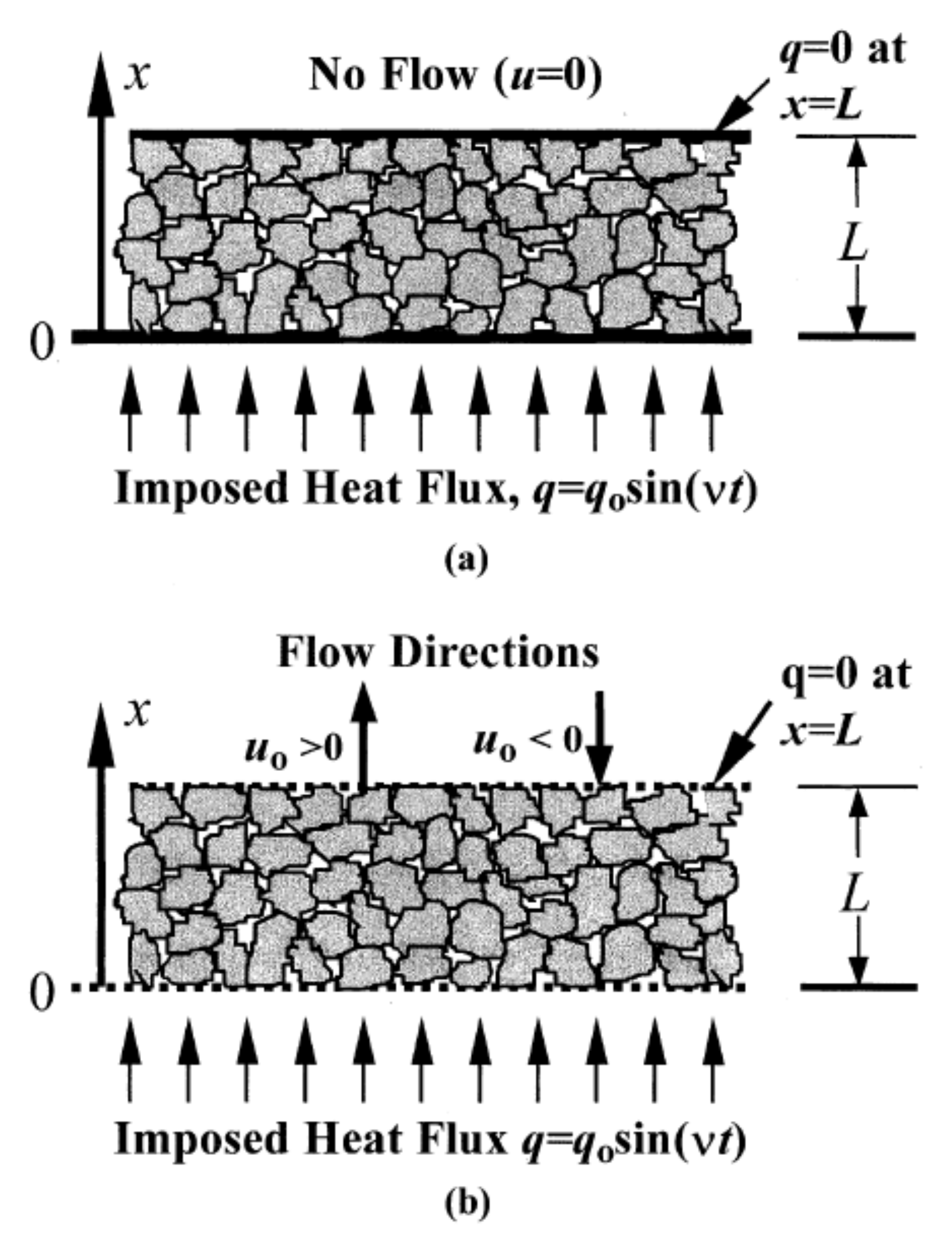
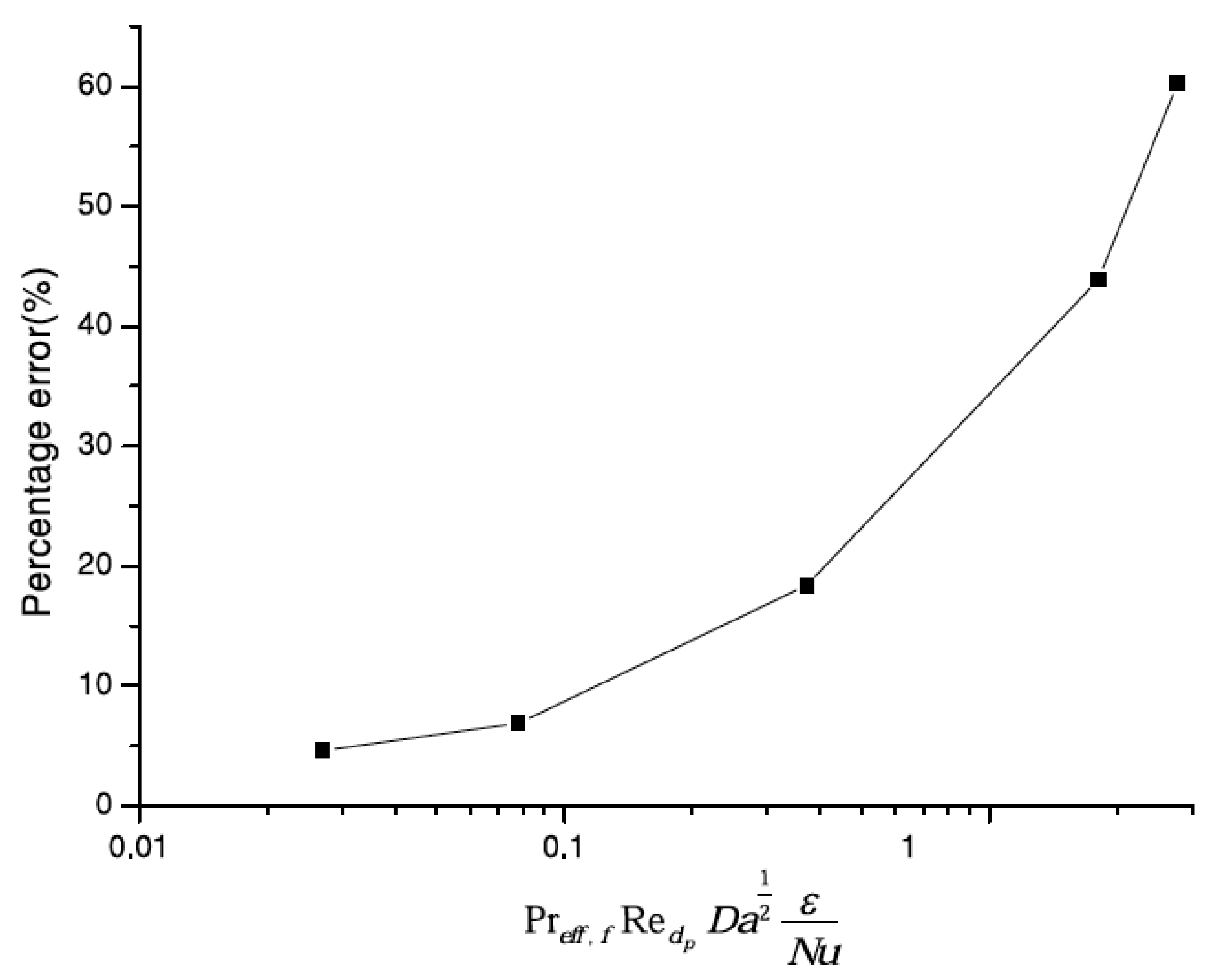
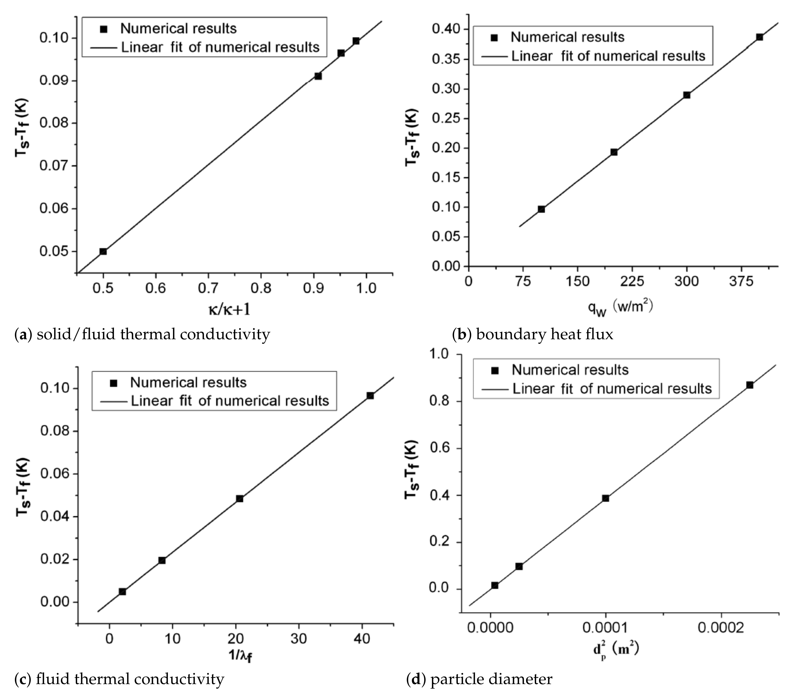
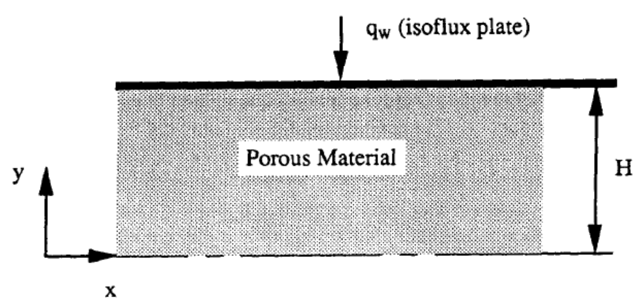
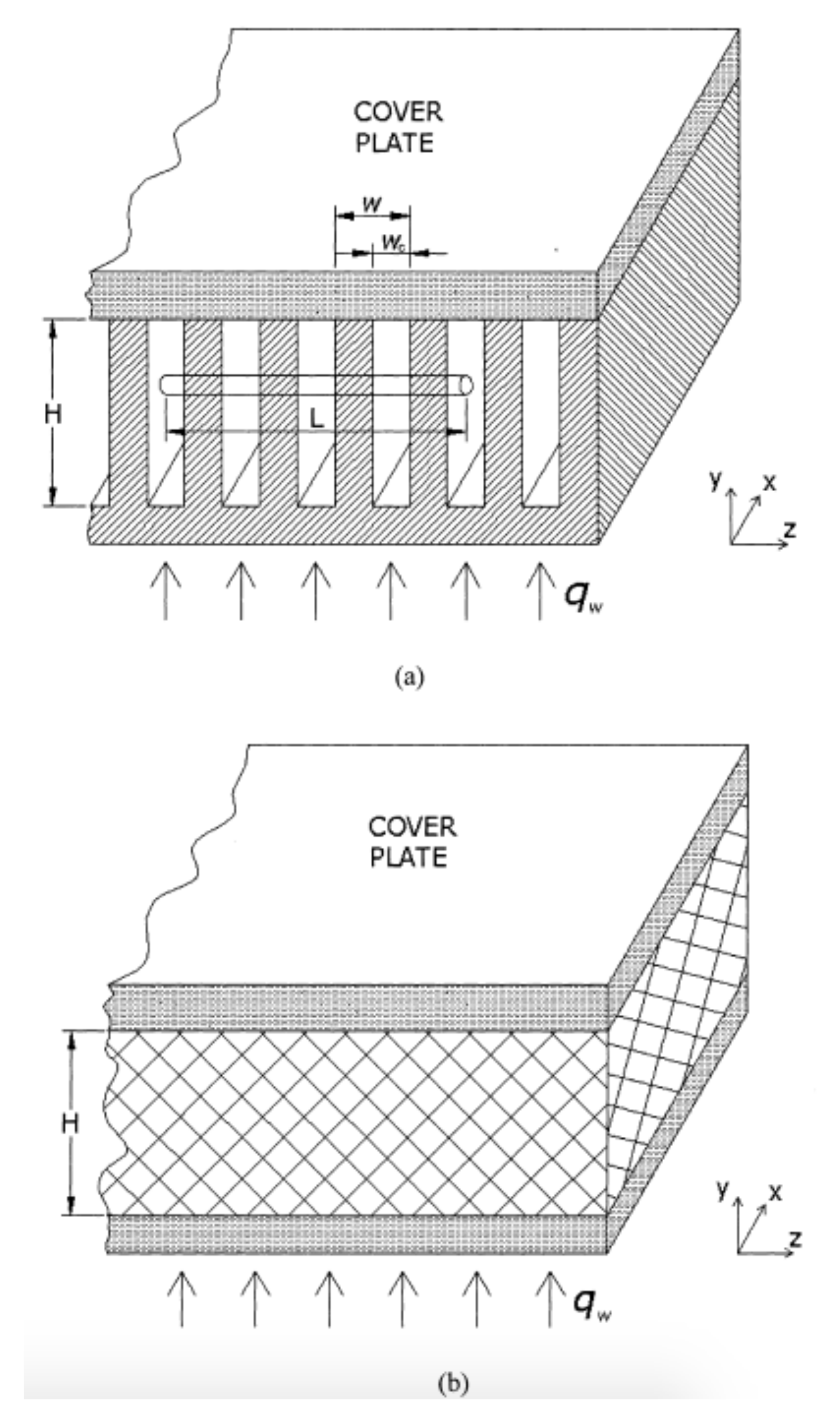
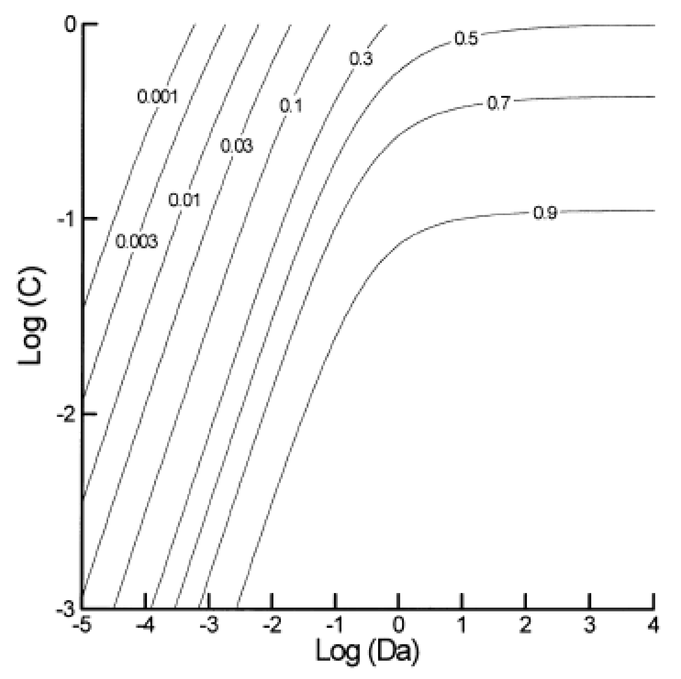
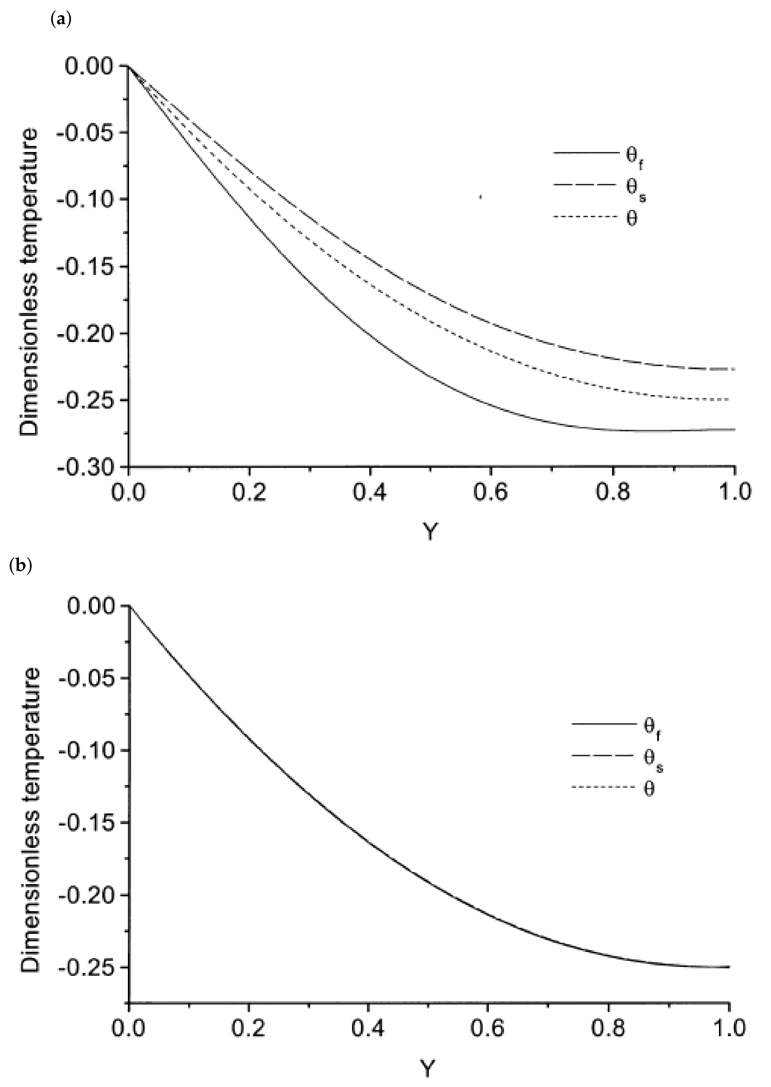
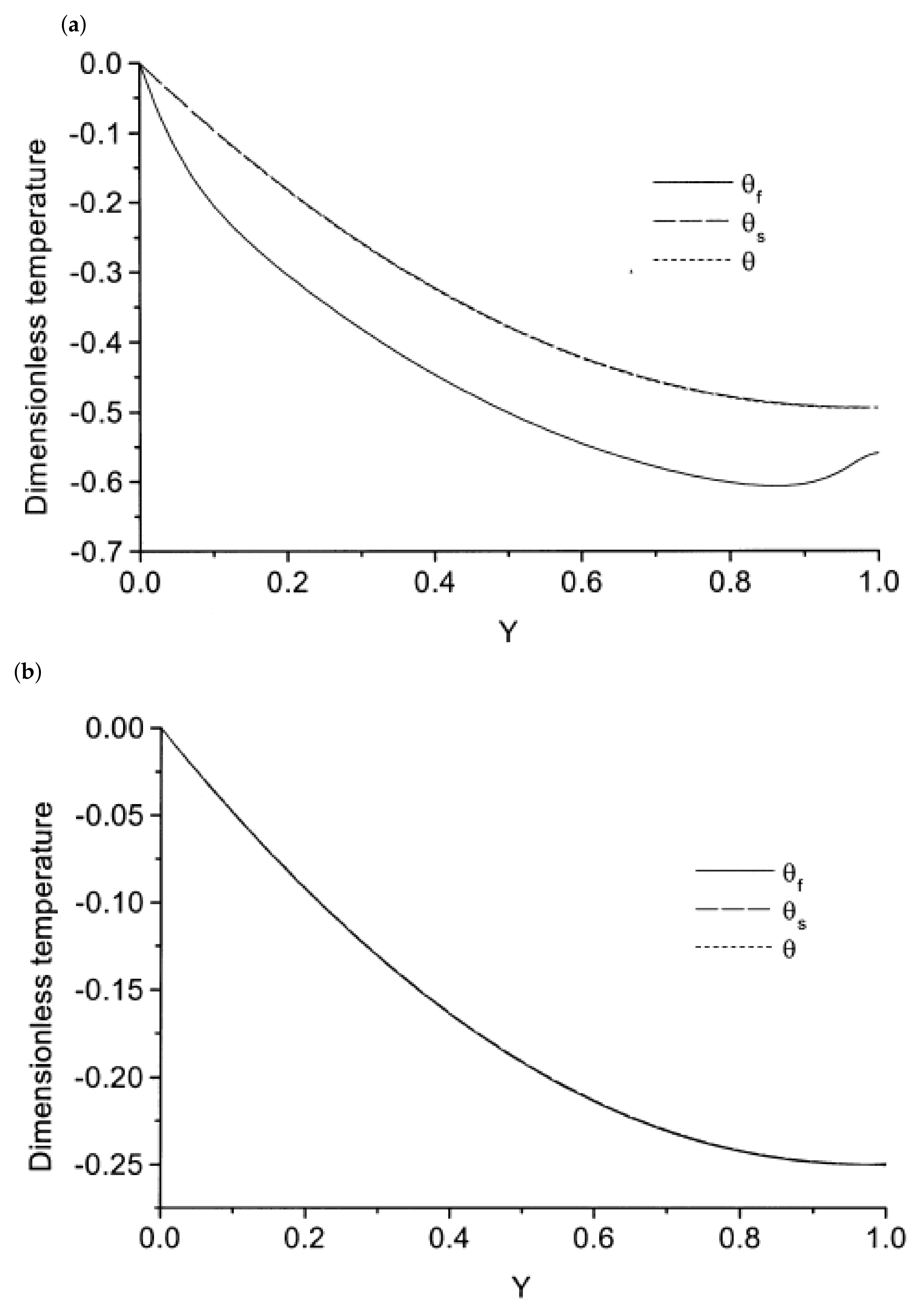
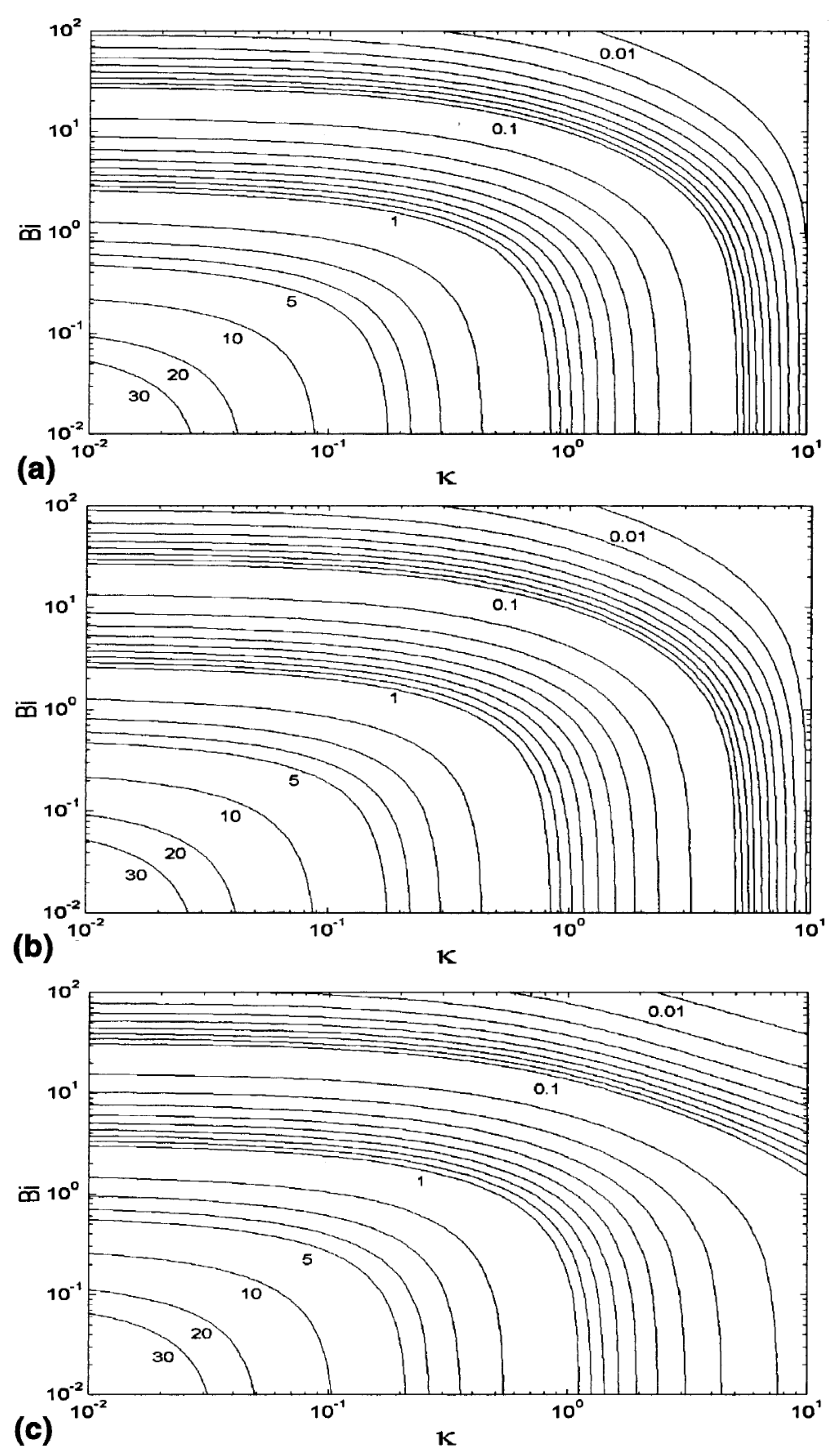
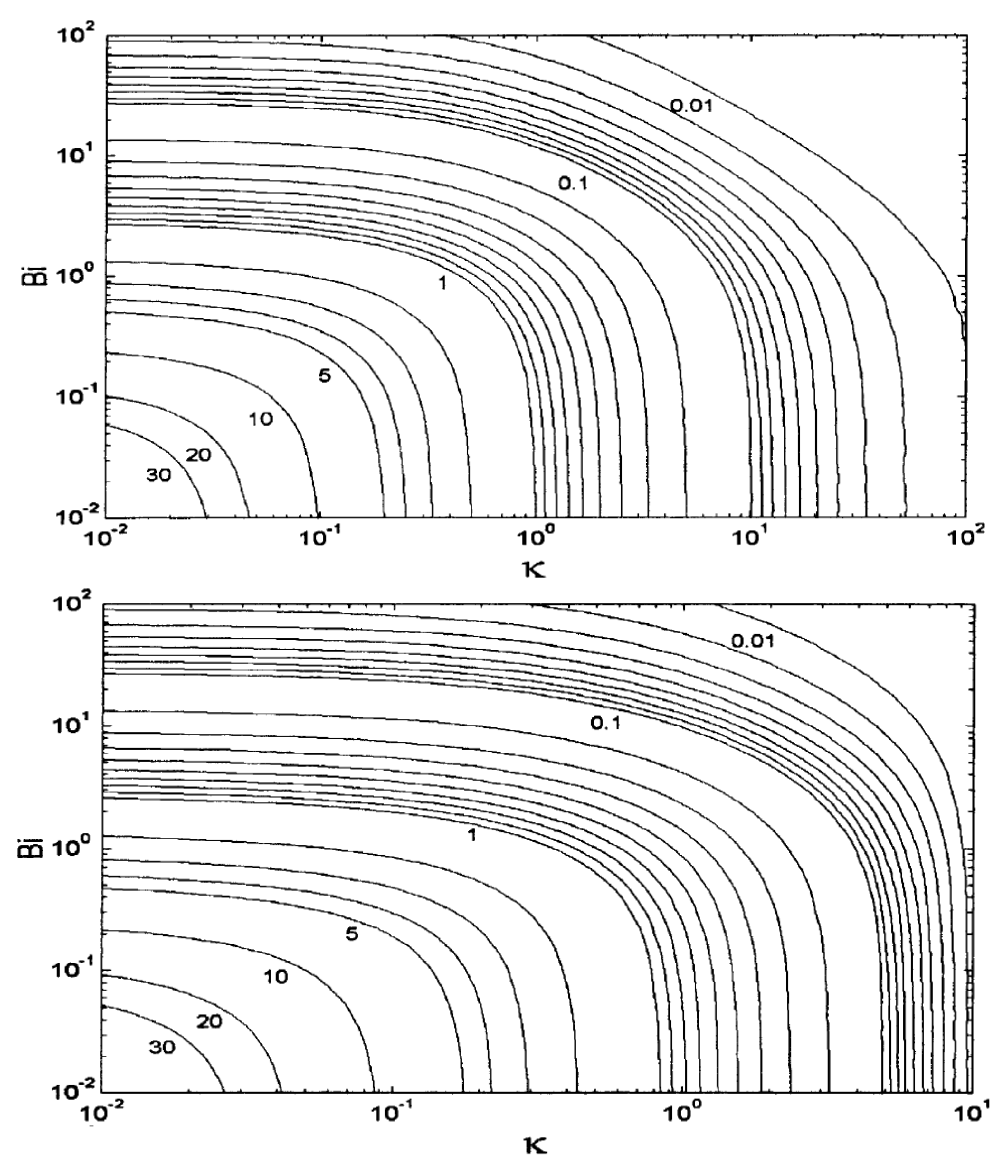
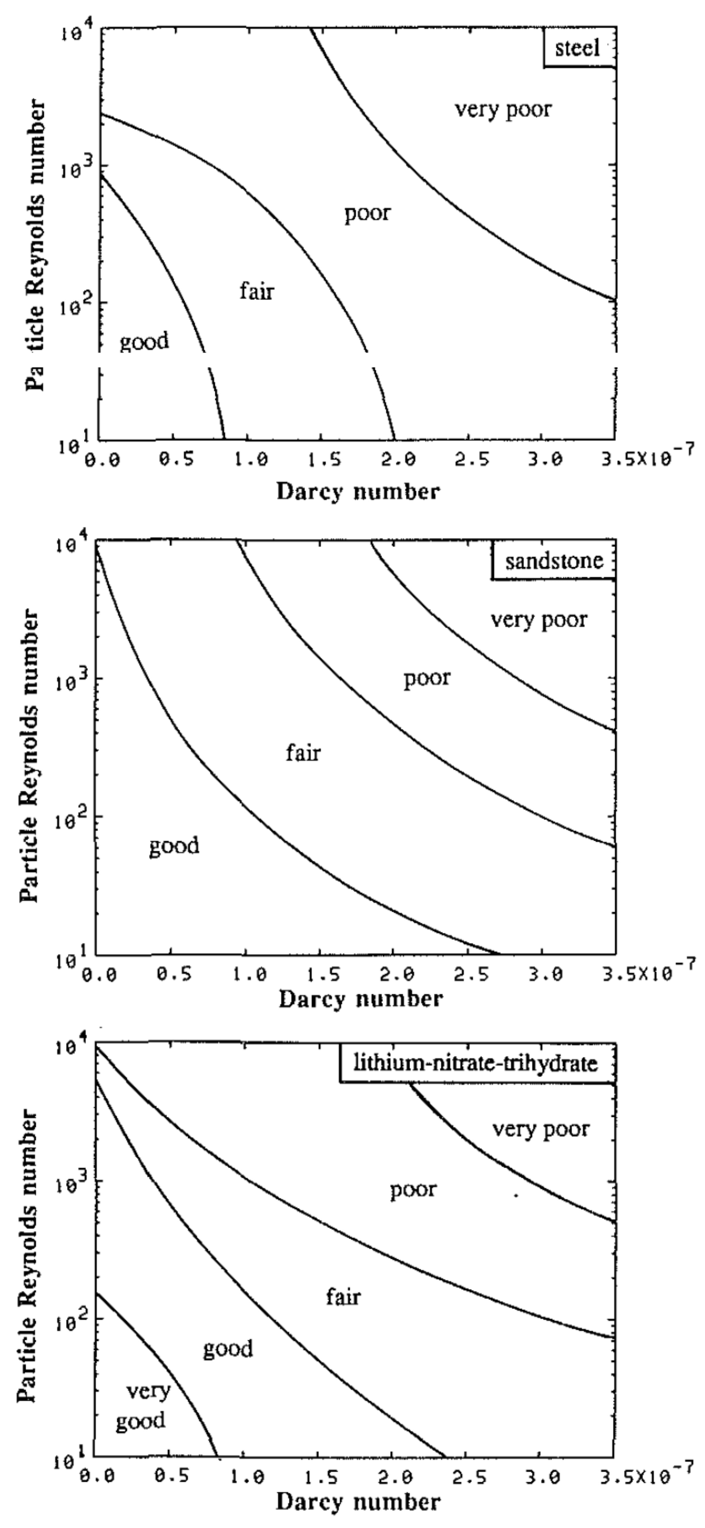
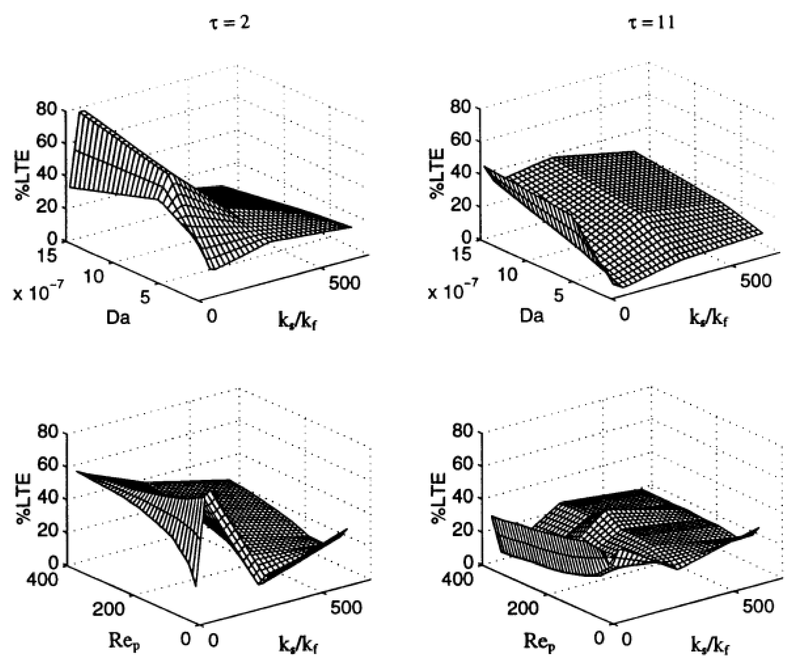
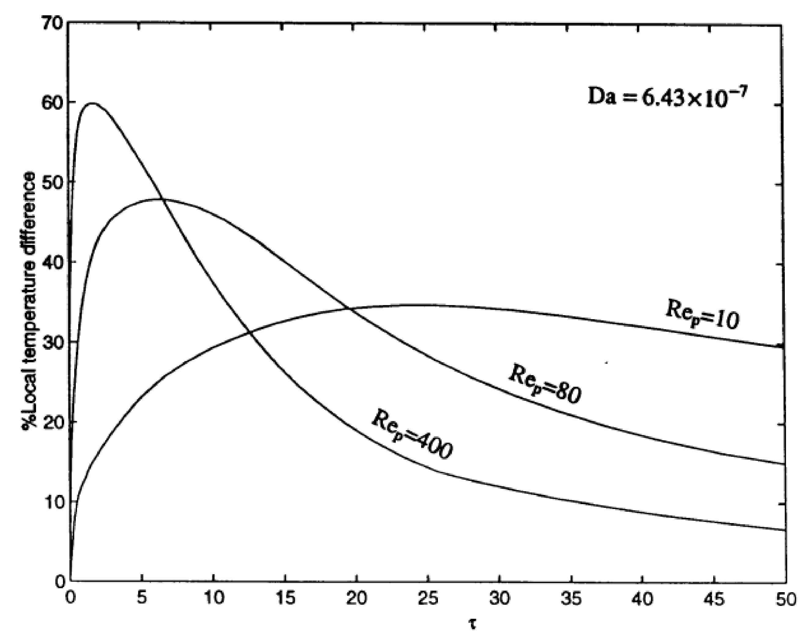
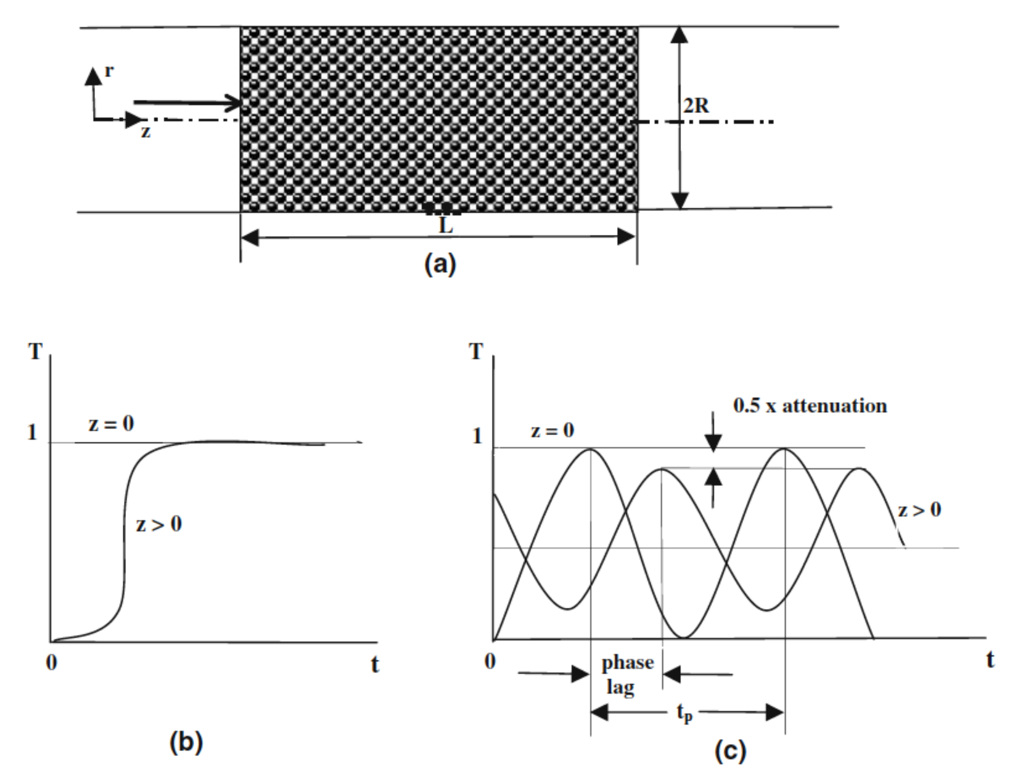
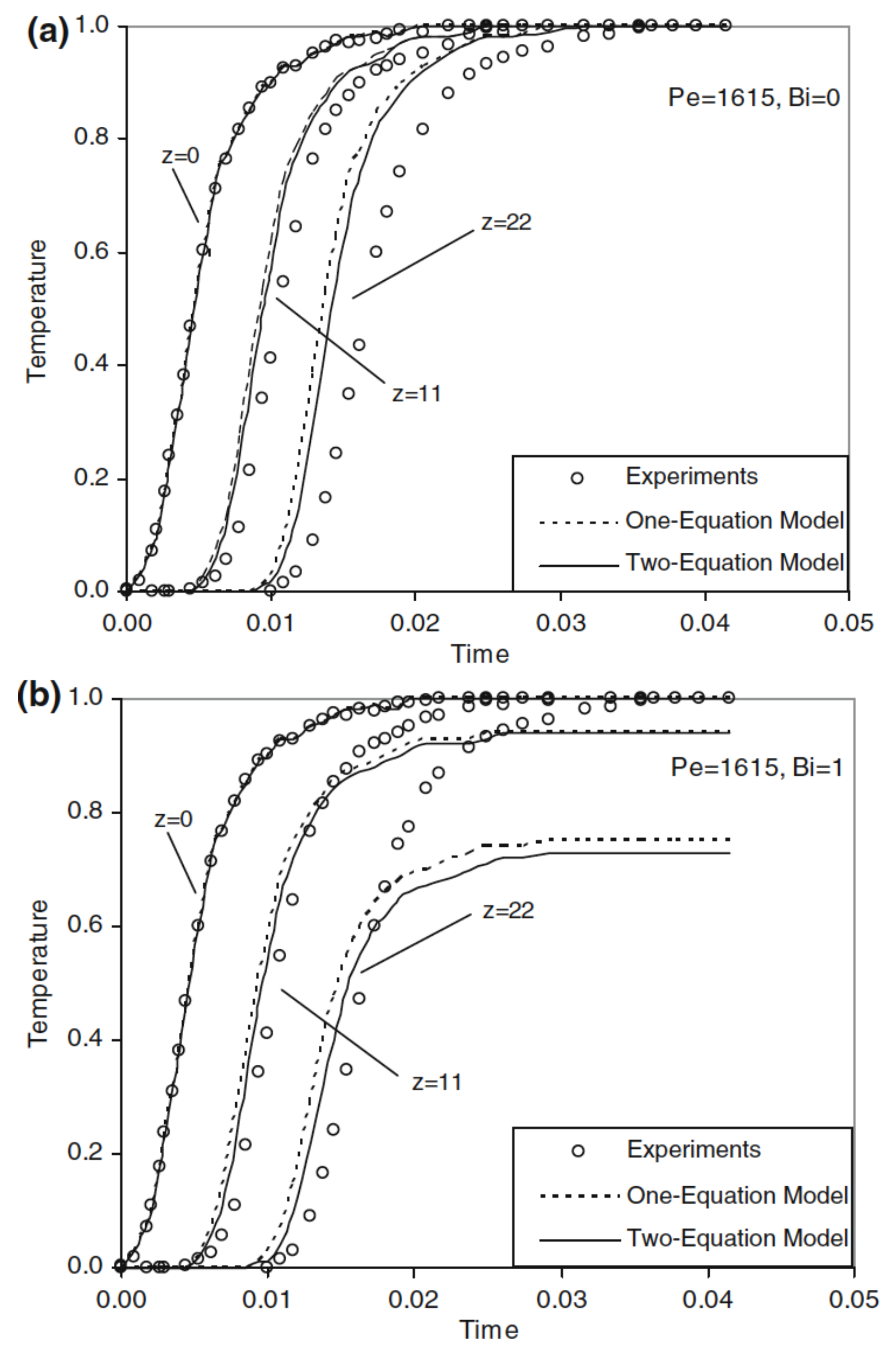
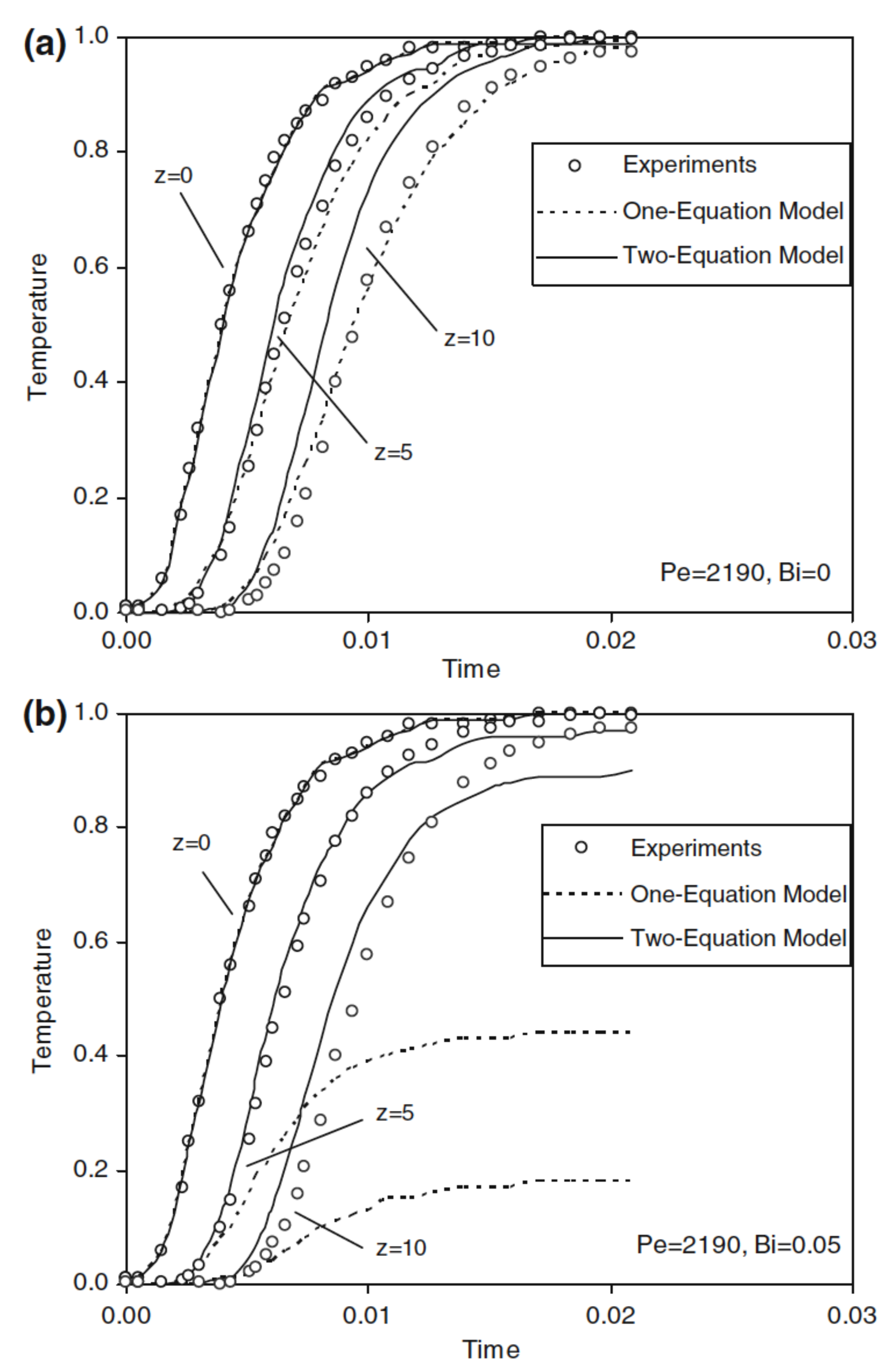
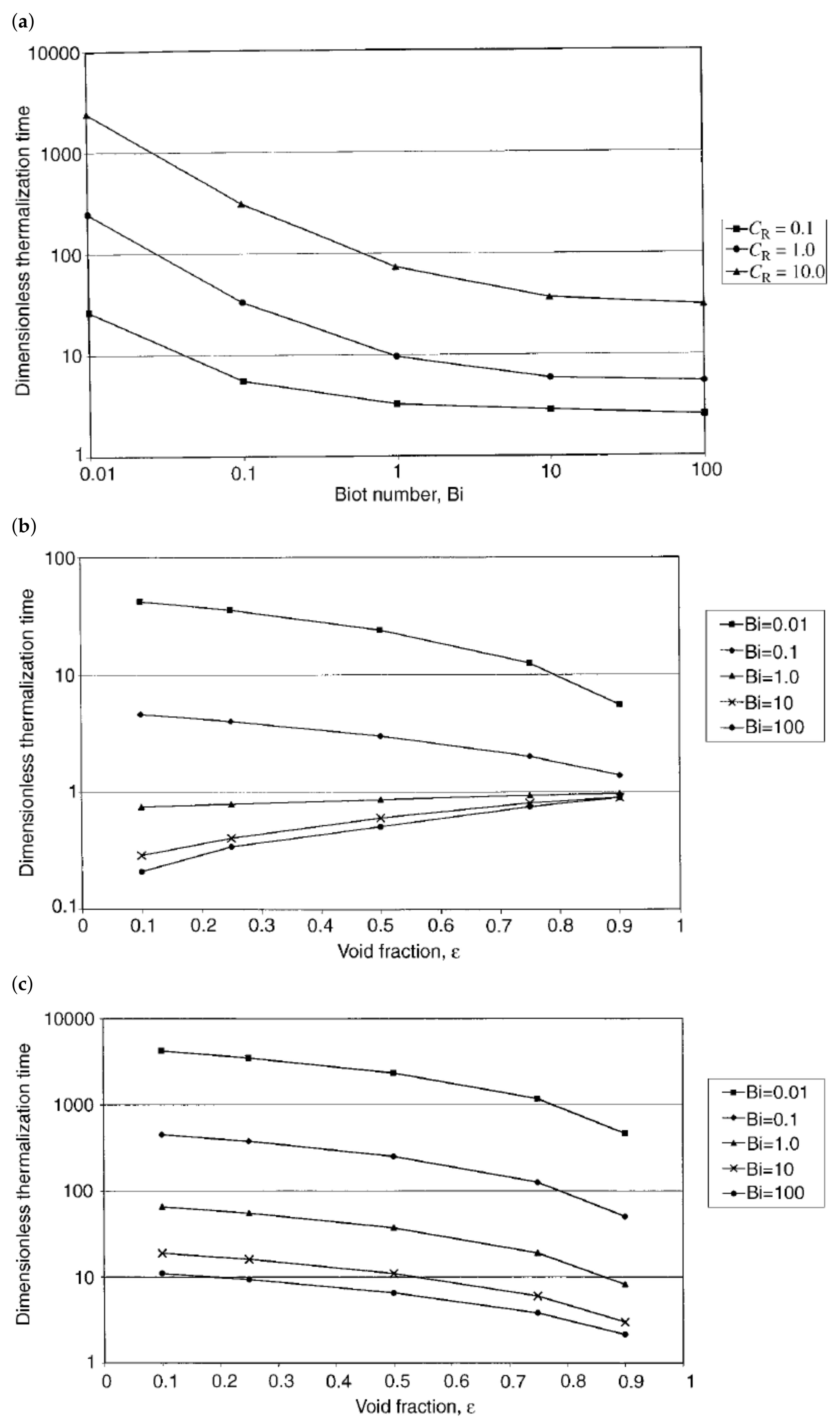
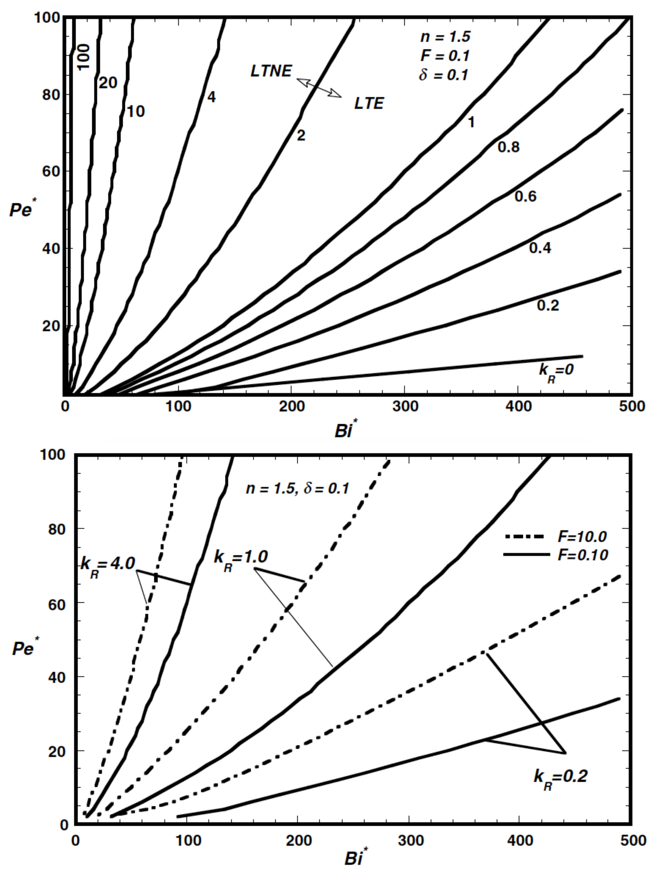
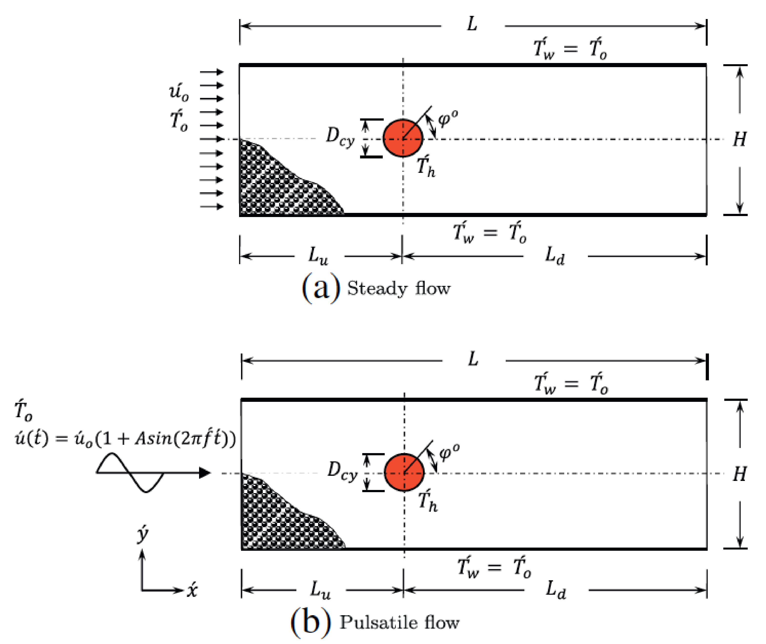
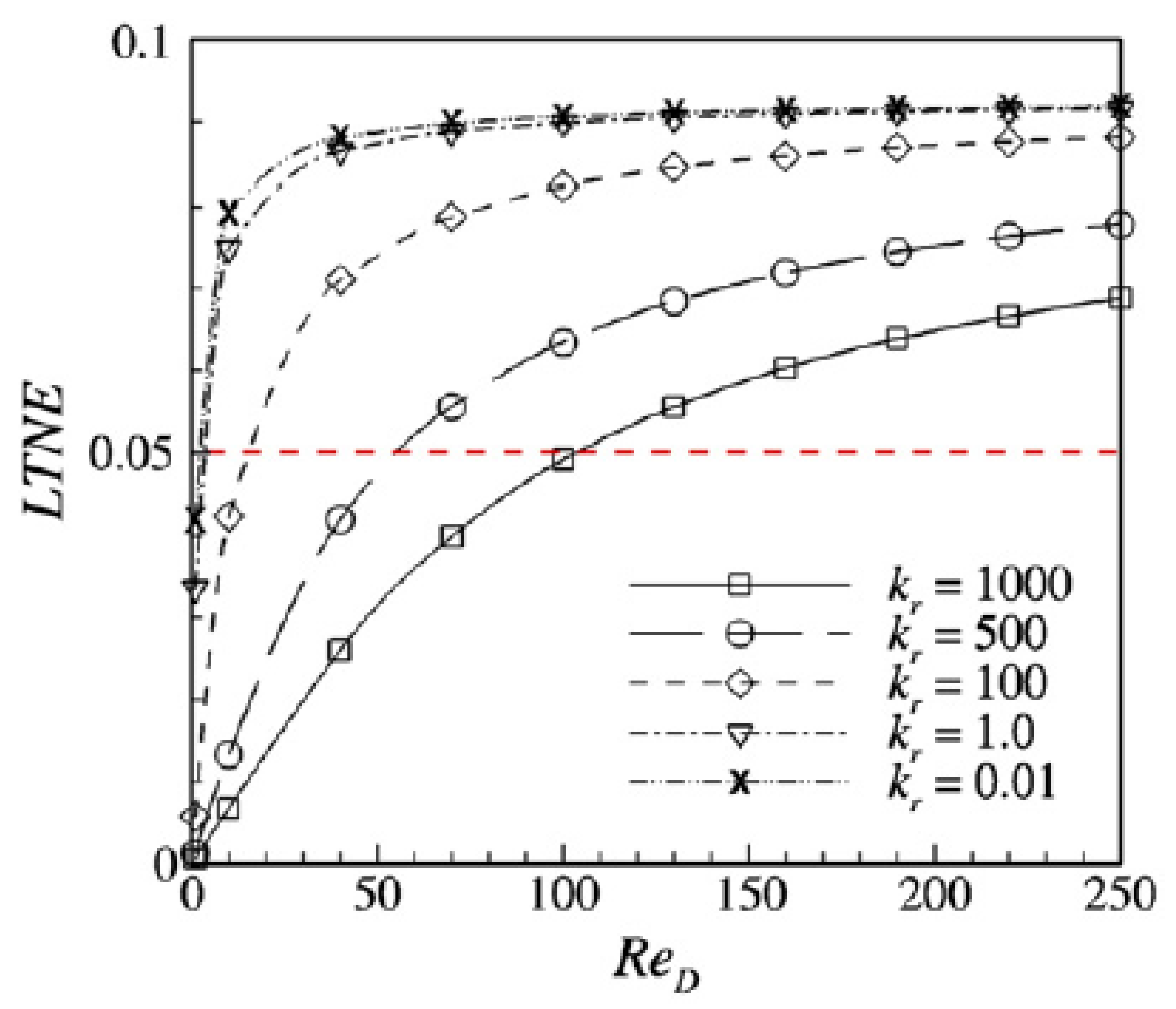
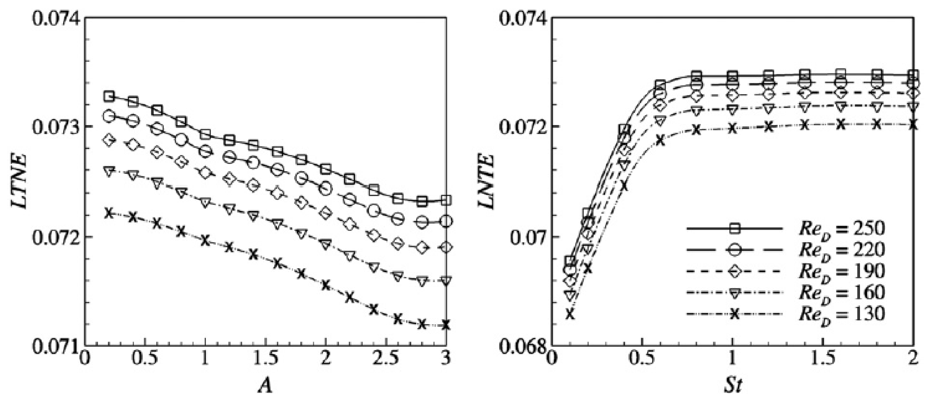
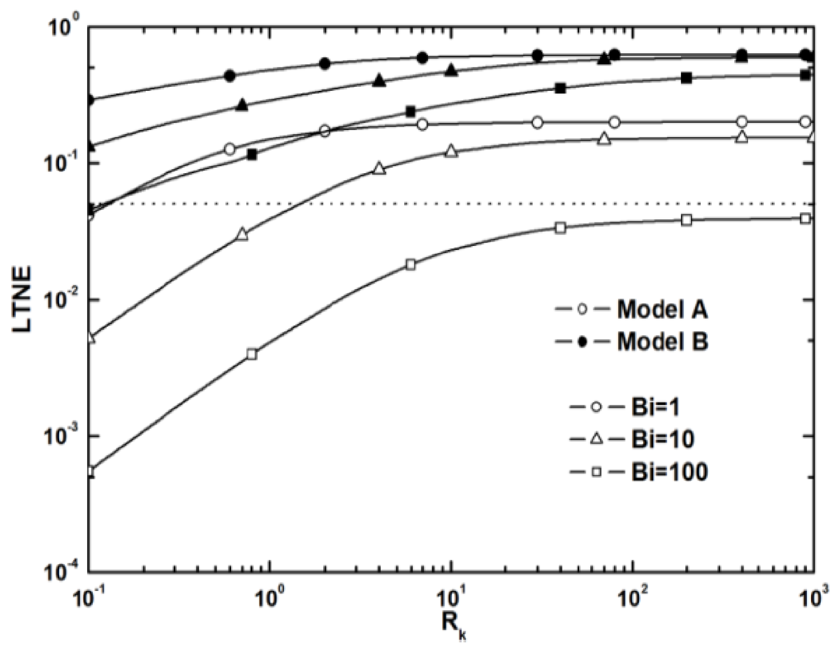
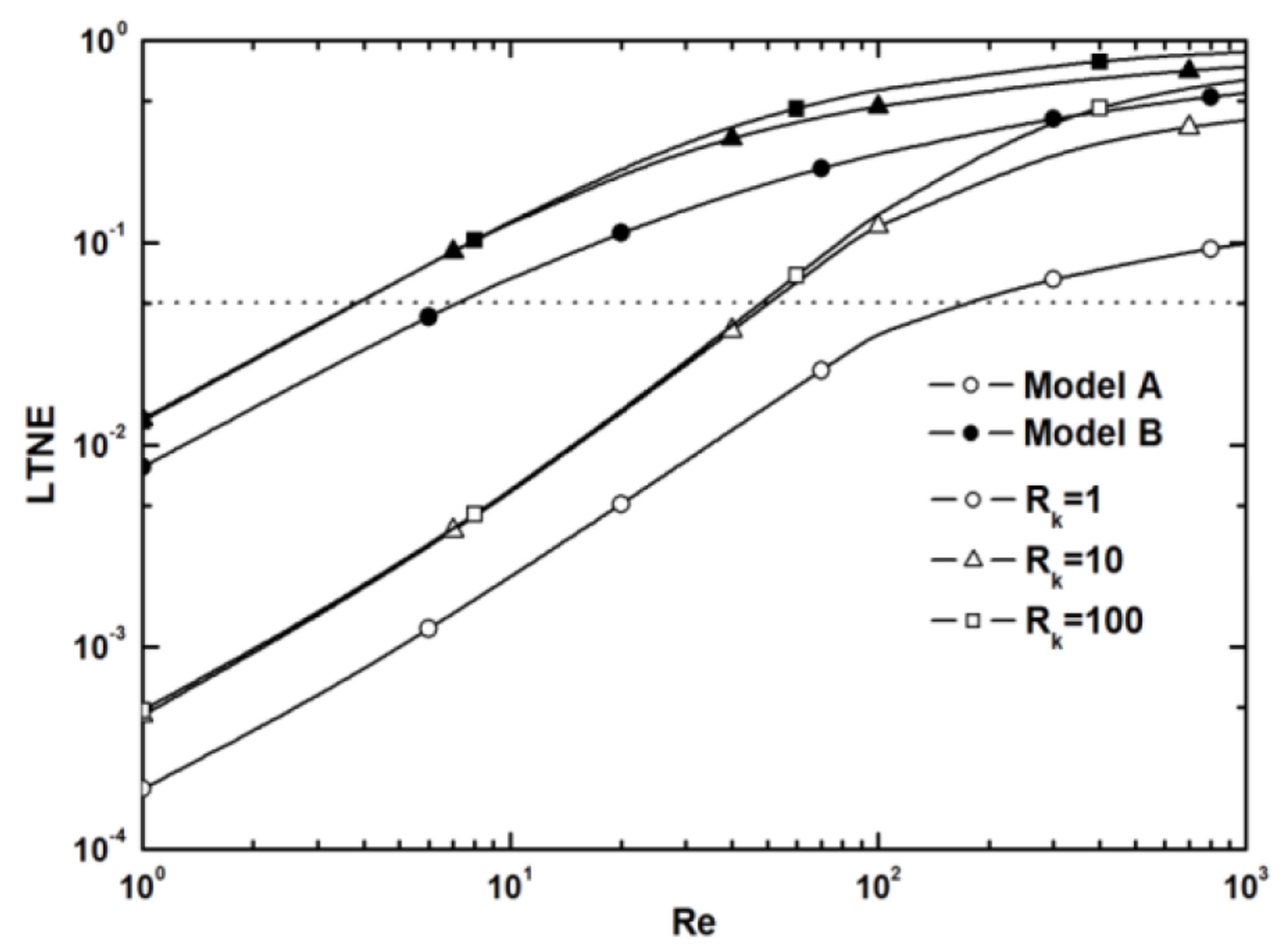
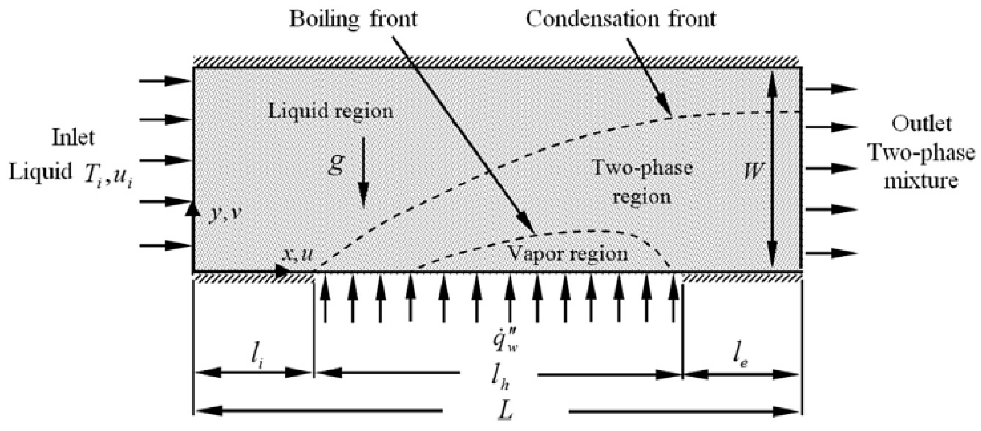
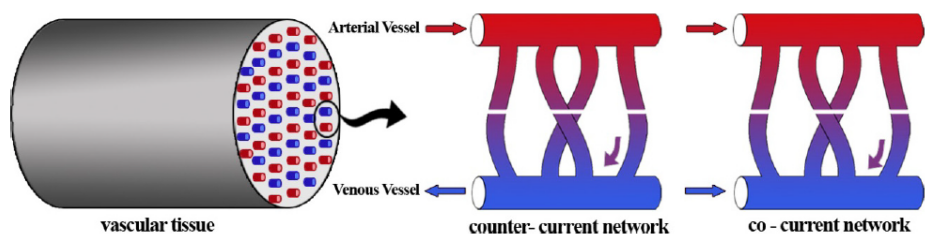
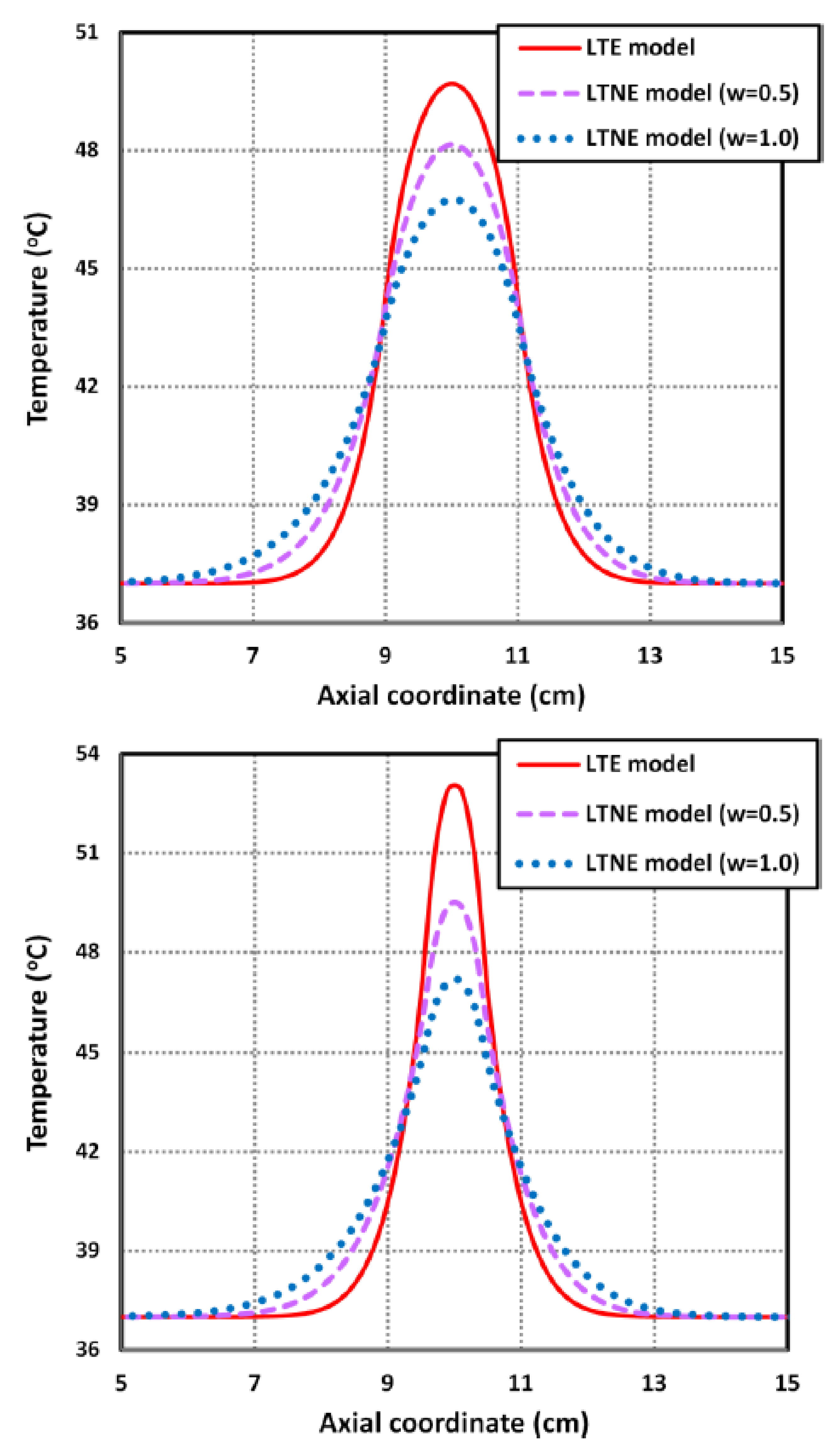
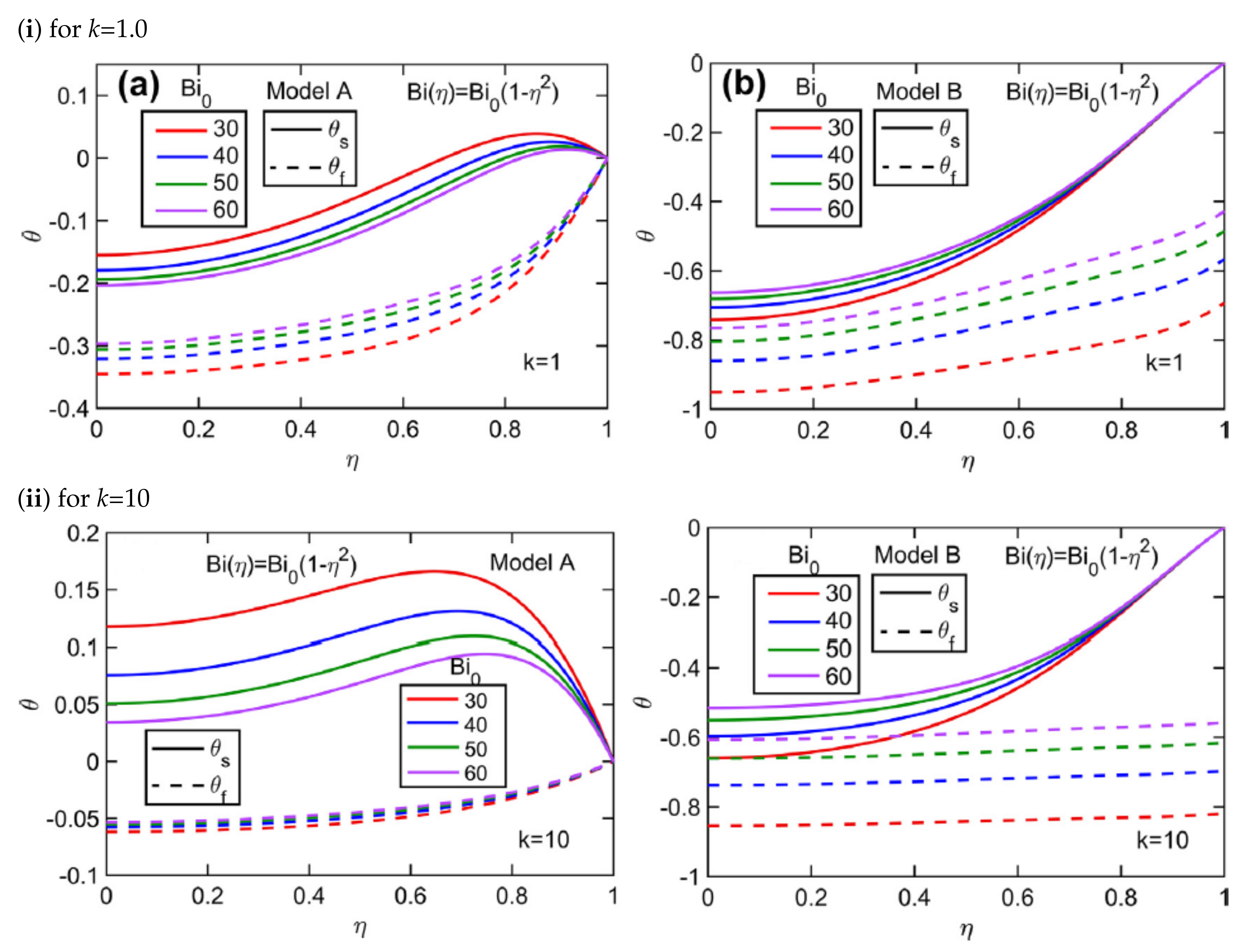
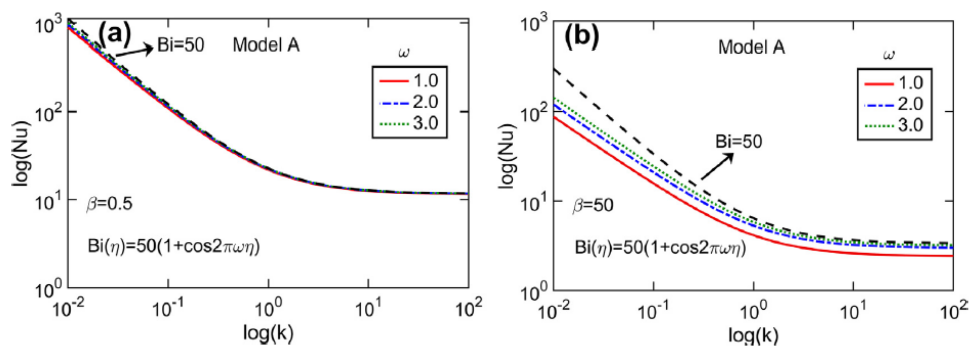
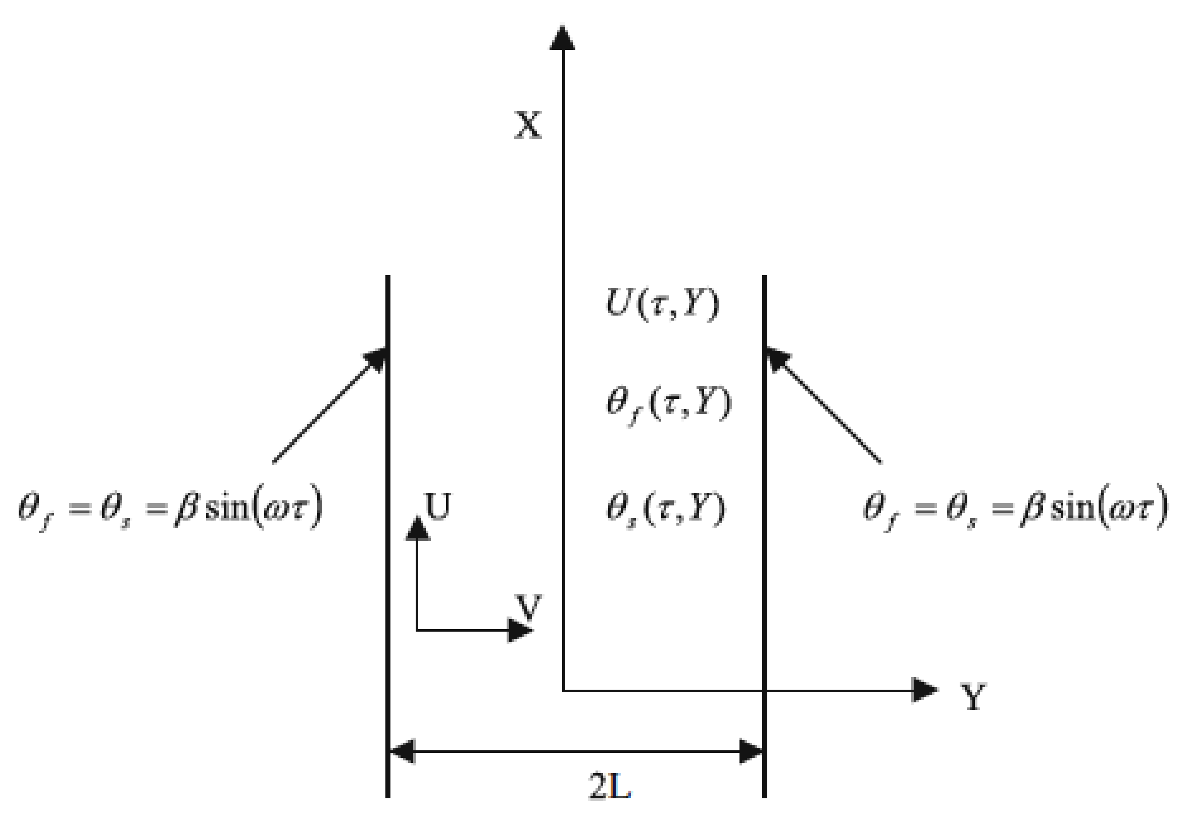
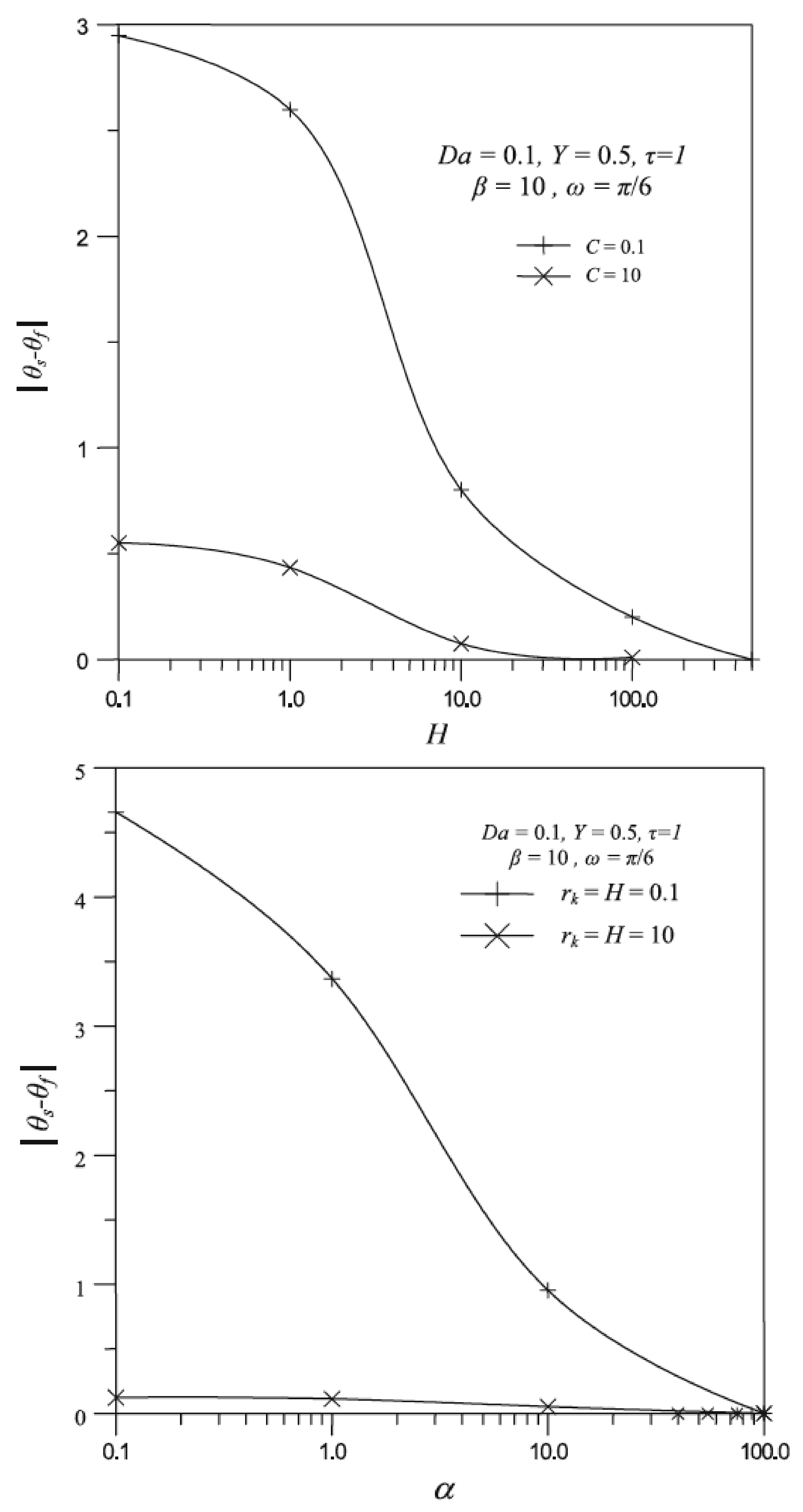
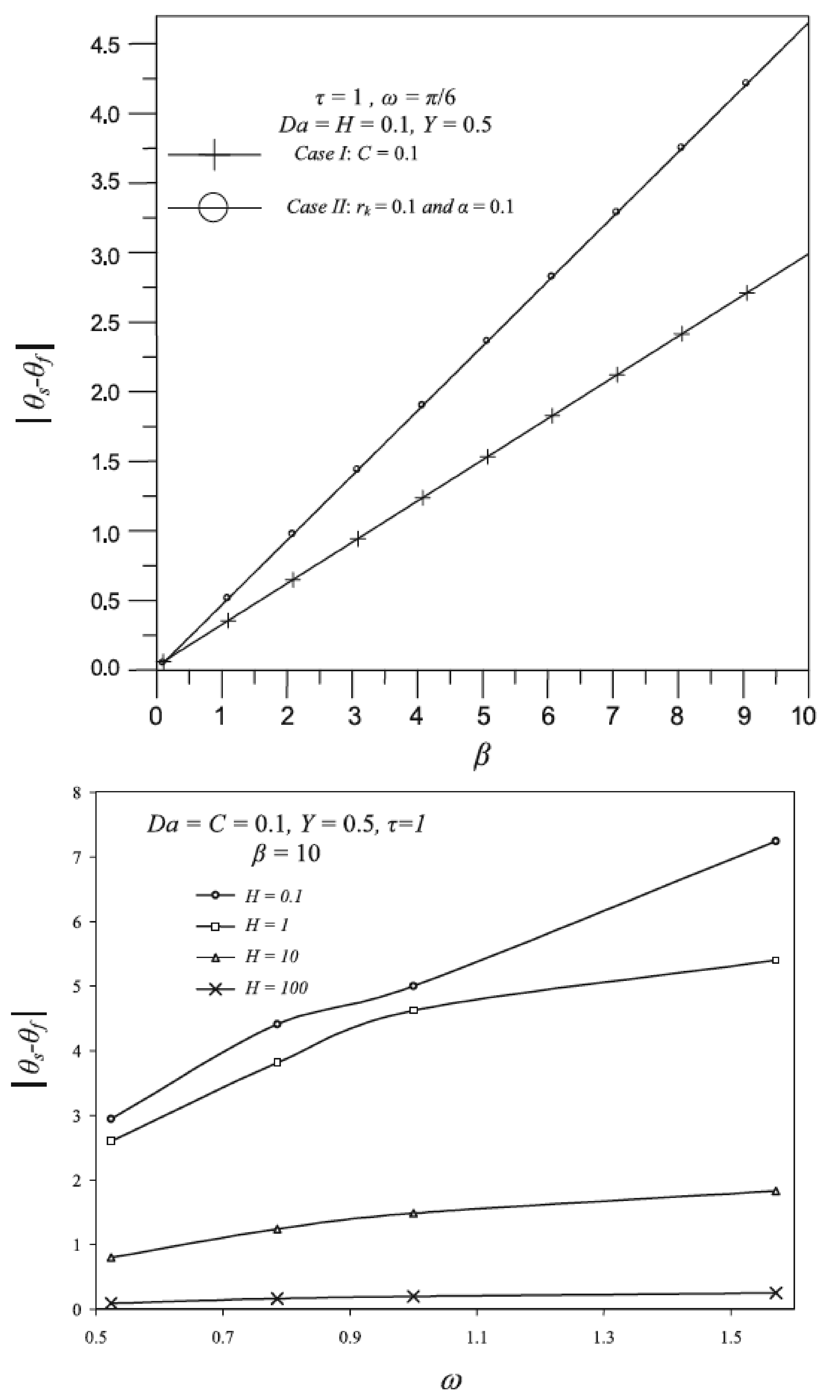
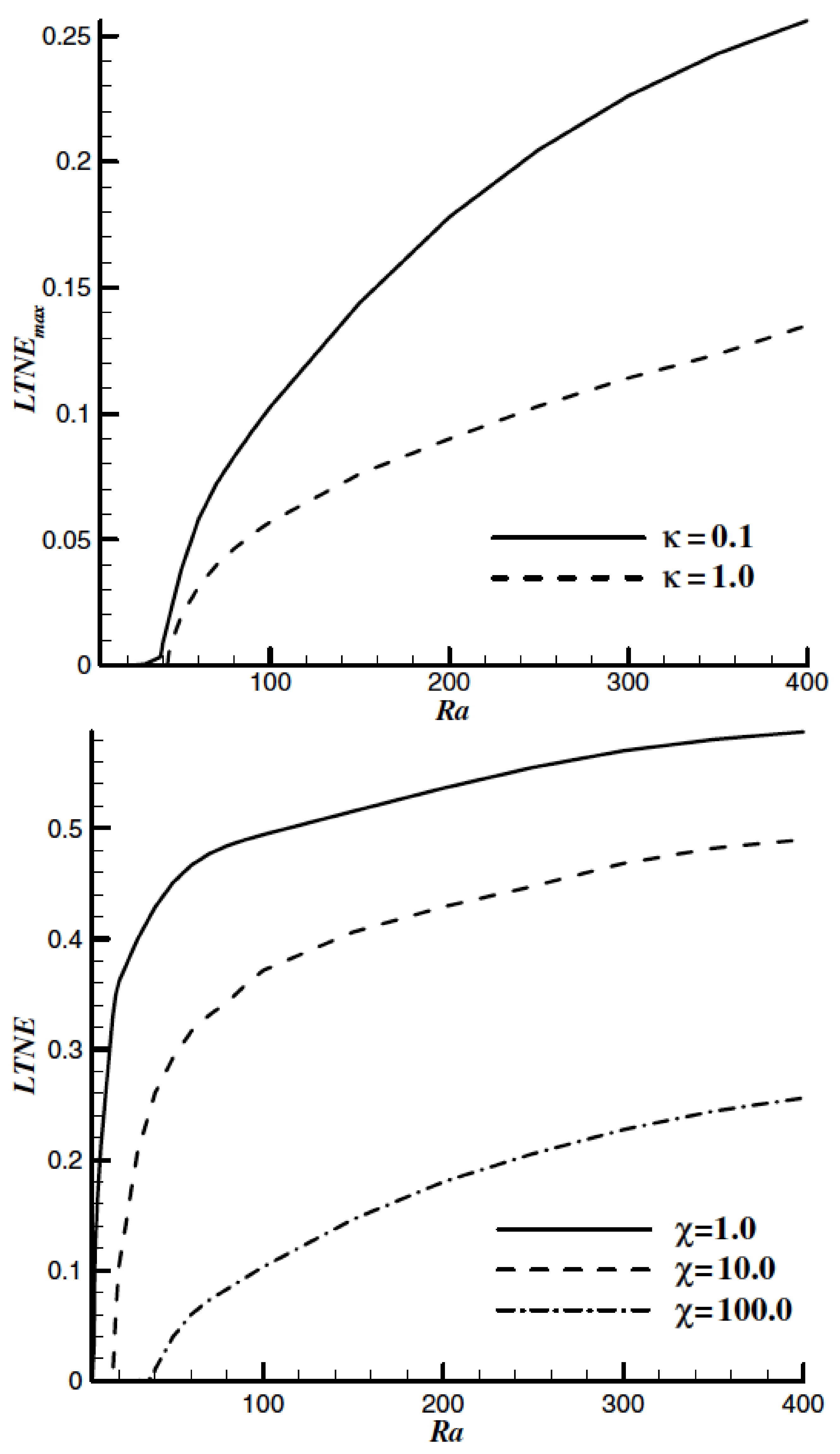
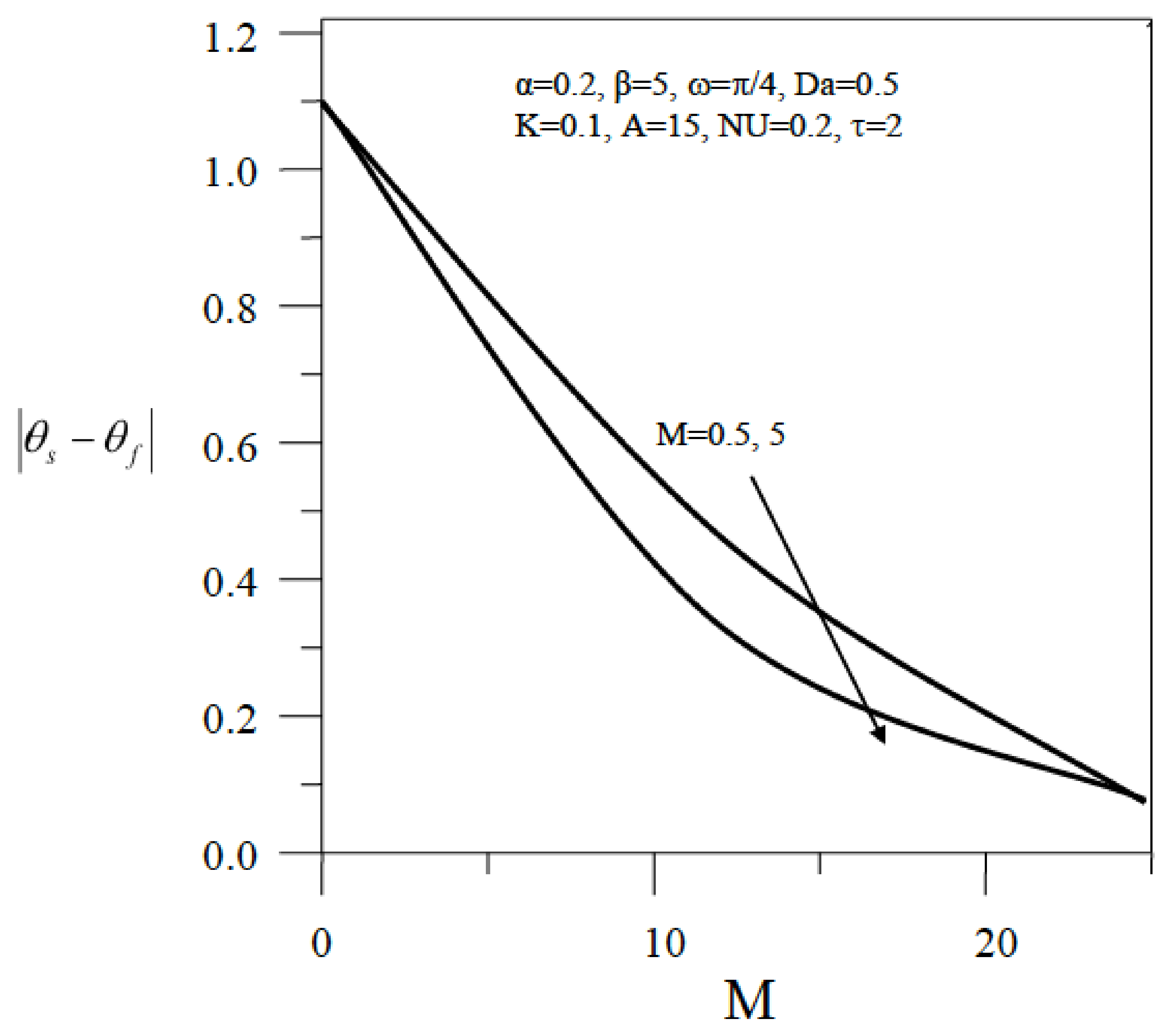
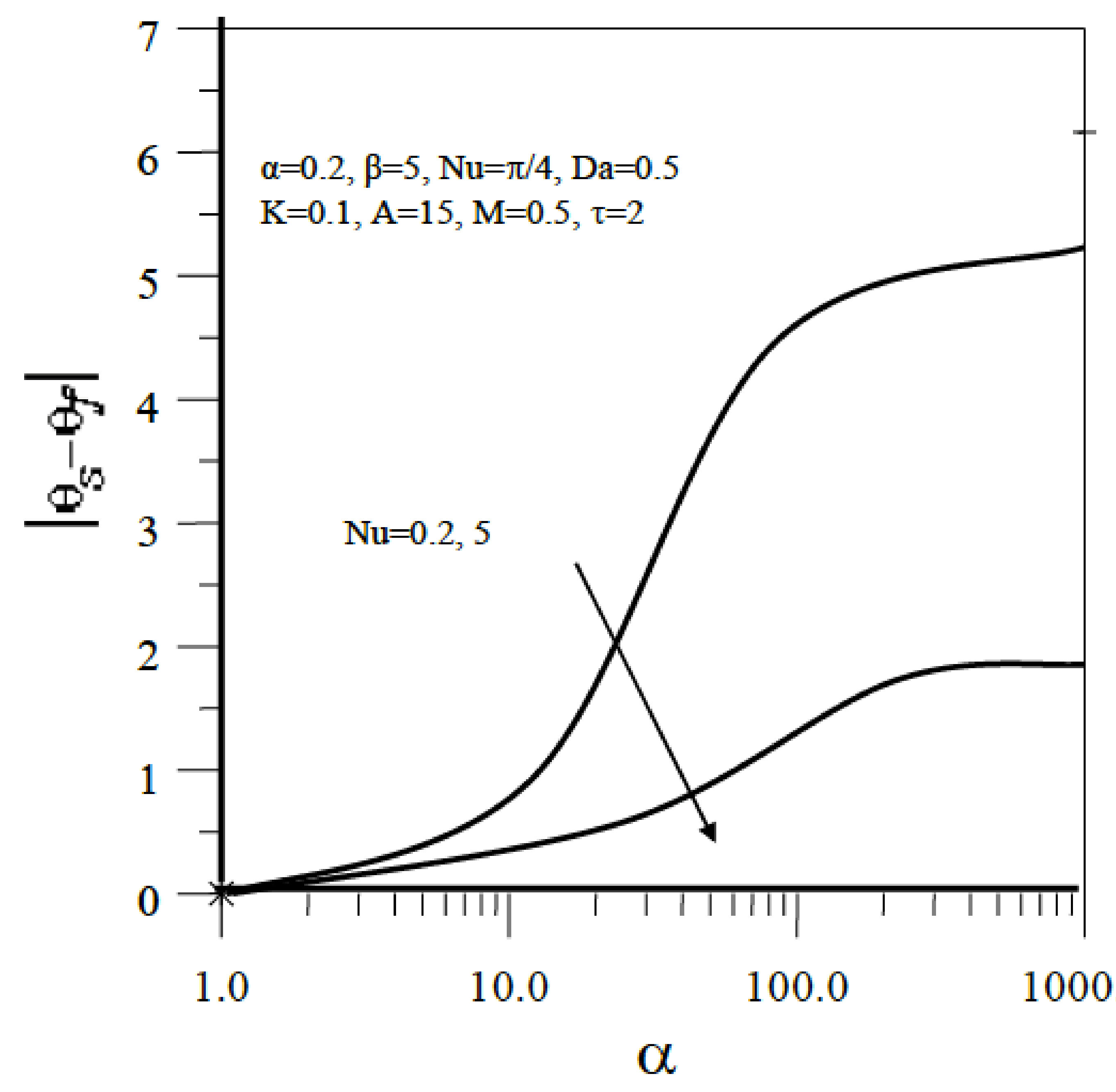
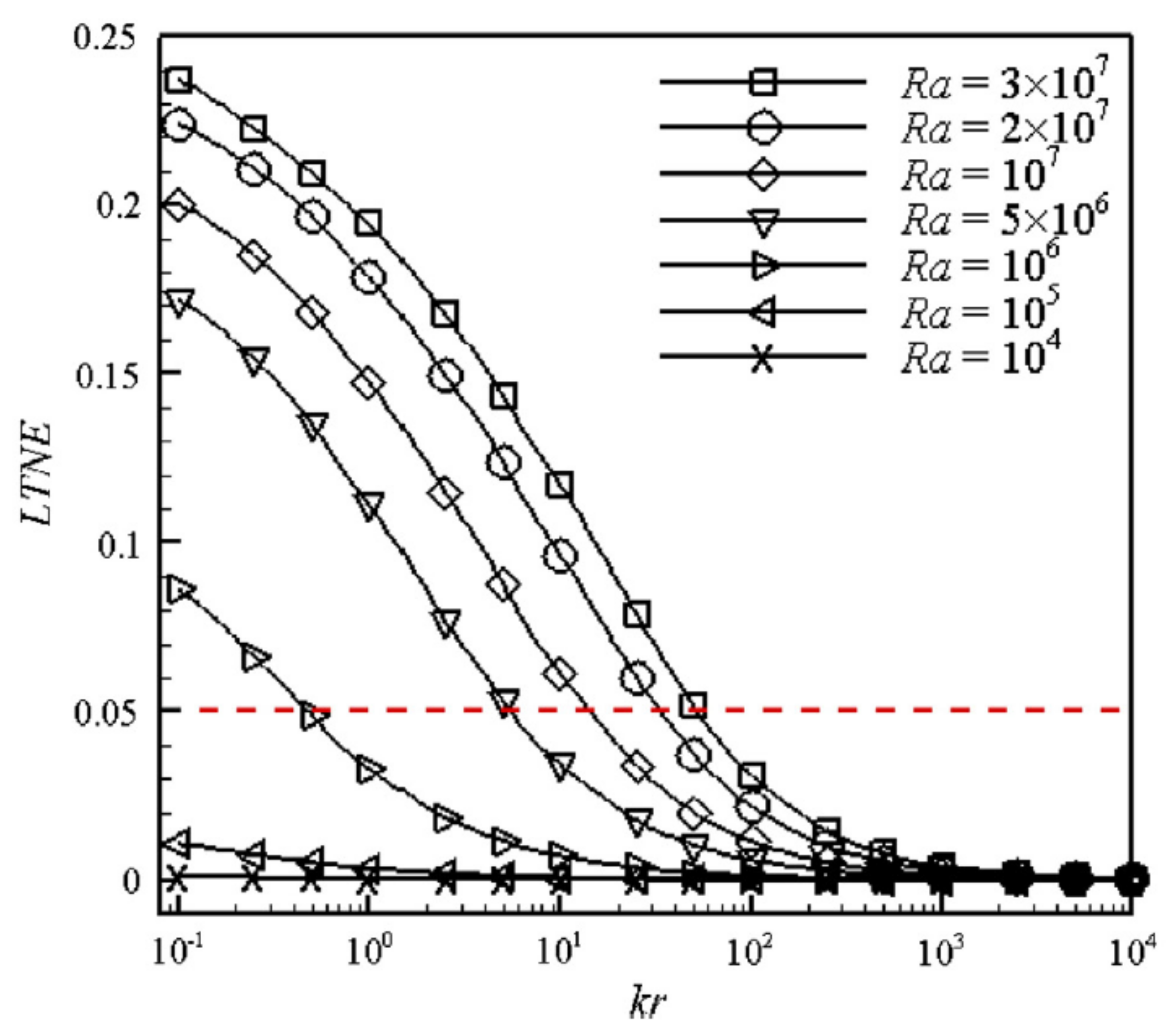
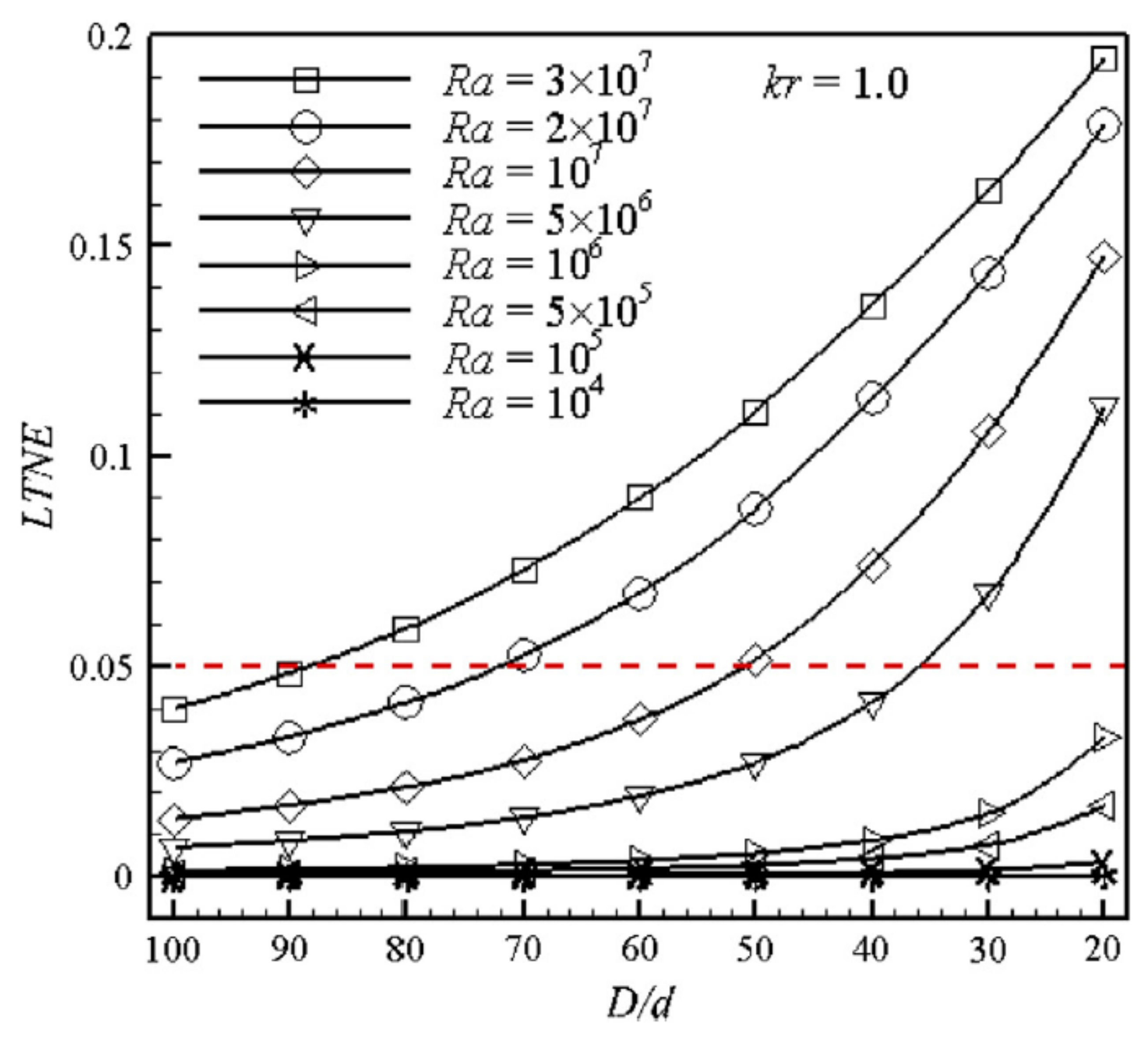
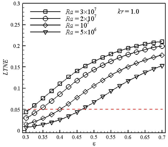
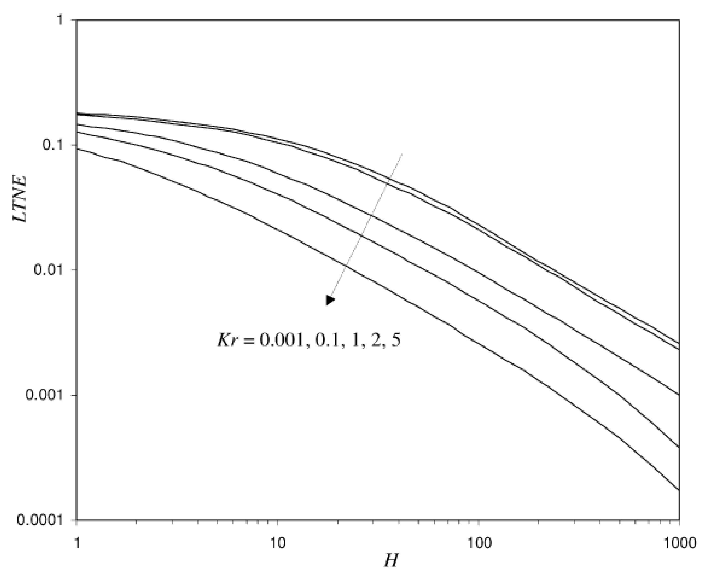
Table 1.
The range of characteristic porous media parameters within which the hypothesis is verified.
Table 1.
The range of characteristic porous media parameters within which the hypothesis is verified.
| Parameters | Investigated by |
|---|---|
| 1 | Quintard and Whitaker [28], Quintard and Whitaker [29], Whitaker [30], Carbonell and Whitaker [31] |
| high | Minkowycz et al. [32] |
| Kim and Jang [33] | |
| Zhang and Liu [34] | |
| ↓, inertia parameter ↑ in fully developed region ↑, inertia parameter ↓ in boundary layer region | Kuznetsov [35] |
| Nield [36] | |
Bi=(hsfasf Hch2//keffs) E… allowable error | Lee and Vafai [37] |
| porosity-scaled fluid/solid thermal conductivity ratio ↑, Da ↓ | Kim et al. [38] |
| Bi ↑, fluid/solid thermal conductivity ratio ↑, inertial parameter , Da ↓ | Marafie and Vafai [39] |
| solid/fluid thermal conductivity ratio →1, and if | Nield et al. [40] |
| particle Re and/or Da ↑, ↓ | Vafai and Sözen [41] |
| either Da or Re → zero, solid/fluid thermal diffusivity ratio ↑ | Amiri and Vafai [42] |
| solid/fluid thermal conductivity ratio → unity, Da ↓, but interestingly for Re ↑ | Amiri and Vafai [43] |
| in glass-water system, as Re ↑ in air-metal system, as Re ↓ for domains of larger length, which need long time scale | Singh et al. [44] |
| For oscillatory thermal response, Pe ↓, amplitude attenuation ↓, phase lag ↓ For steady thermal response, when Bi = | Singh et al. [45] |
| when the thermal equilibrium relaxation time () ⋘ the time scale of the physical case, and ↓ as Bi ↑ or as fluid/solid thermal capacity ratio ↓ ↓ as ↑ for small Bi and large | Al-Nimr and Abu-Hijleh [46] |
| as Pe ↓, macroscopic frictional coefficient ↑, Forchheimer parameter ↑, power-law fluid index ↑, Bi ↑, fluid/solid thermal conductivity ratio ↑ | Khashan and Al-Nimr [47] |
| as Pe ↓, Re ↓, Da ↓, fluid/solid conductivity ratio ↓, or as Forchheimer coefficient ↑, Bi ↑ | Khashan et al. [48] |
| for steady flow, as Pr ↓, Re ↓, Bi ↑, Da ↑, cylinder/particle diameter ratio ↑, solid/fluid thermal conductivity ratio ↑, ↑, for pulsatile flow, as Strouhal number ↓ or as oscillating amplitude ↑ | Al-Sumaily et al. [49] |
| as interphase convective heat transfer parameter () ↑, porosity scaled fluid/solid thermal conductivity ratio () ↑ | Wong and Saeid [50] |
| as solid/fluid thermal conductivity ratio ↓, Pr ↓, Re ↓, Bi ↑, ↑ | Abdedou and Bouhadef [51] |
| when the blood perfusion rate during the tissue ↓, or the heat source intensity ↓ | Hassanpour and Saboonchi [53] |
| when , or as the interior heat generation parameter ↓ | Parhizi et al. [55] |
| higher Bi↑, Da↑, , Ra↓ | Haddad et al. [56] |
| as interfacial heat transfer parameter , thermal capacity ratio , thermal conductivity ratio , thermal diffusivity ratio , or as the amplitude and/or the frequency of the thermal disturbance ↓ | Khadrawi et al. [57] |
| as Da↓, Ra↓, or as Bi↑, effective fluid/solid thermal conductivity ratio ↑ | Khashan et al. [58] |
| as magnetic field parameter (M) ↑, interphase convective heat transfer parameter ↑, solid/fluid thermal conductivity ratio ↑, thermal diffusivity ratio ()↓, fluctuation amplitudes and frequencies ↓ | Tahat et al. [59] |
| as interphase convective coefficient ↑, fluid/solid conductivity ratio ↑, permeability ratio ↑, and wall thickness ↑, solid/fluid heat capacity ratio ↓ | Harzallah et al. [60] |
| solid/fluid conductivity ratio ↑, cylinder/particle diameter ratio ↑, Ra↓, | Al-Sumaily et al. [61] |
| as interfacial convective heat transfer parameter () ↑, porosity scaled fluid/solid thermal conductivity ratio () ↑, Ra↓, wall heat flux ↓ | Bourouis et al. [62] |
Publisher’s Note: MDPI stays neutral with regard to jurisdictional claims in published maps and institutional affiliations. |
© 2021 by the authors. Licensee MDPI, Basel, Switzerland. This article is an open access article distributed under the terms and conditions of the Creative Commons Attribution (CC BY) license (https://creativecommons.org/licenses/by/4.0/).
Share and Cite
MDPI and ACS Style
Al-Sumaily, G.F.; Al Ezzi, A.; Dhahad, H.A.; Thompson, M.C.; Yusaf, T. Legitimacy of the Local Thermal Equilibrium Hypothesis in Porous Media: A Comprehensive Review. Energies 2021, 14, 8114. https://doi.org/10.3390/en14238114
AMA Style
Al-Sumaily GF, Al Ezzi A, Dhahad HA, Thompson MC, Yusaf T. Legitimacy of the Local Thermal Equilibrium Hypothesis in Porous Media: A Comprehensive Review. Energies. 2021; 14(23):8114. https://doi.org/10.3390/en14238114
Chicago/Turabian StyleAl-Sumaily, Gazy F., Amged Al Ezzi, Hayder A. Dhahad, Mark C. Thompson, and Talal Yusaf. 2021. "Legitimacy of the Local Thermal Equilibrium Hypothesis in Porous Media: A Comprehensive Review" Energies 14, no. 23: 8114. https://doi.org/10.3390/en14238114
Note that from the first issue of 2016, this journal uses article numbers instead of page numbers. See further details here.