Influence of Efficiency, Aging and Charging Strategy on the Economic Viability and Dimensioning of Photovoltaic Home Storage Systems

Abstract

PV in combination with Li-ion storage systems can make a major contribution to the energy transition. However, large-scale application will only take place when the systems are economically viable. The profitability of such a system is not only influenced by the investment costs and economic framework conditions, but also by the technical parameters of the storage systems. The paper presents a methodology for the simulation and sizing of PV home storage systems that takes into account the efficiency of the storage systems (AC, DC standby consumption and peripheral consumption, battery efficiency and inverter efficiency), the aging of the components (cyclic and calendar battery aging and PV degradation), and the intelligence of the charging strategy. The developed methodology can be applied to all regions. In this paper, a sensitivity analysis of the influence of the mentioned technical parameters on the dimensioning and profitability of a PV home storage is performed. The calculation is done for Germany. Especially, battery aging, battery inverter efficiency and a charging strategy to avoid calendar aging have a decisive influence. While optimization of most other technical parameters only leads to a cost reduction of 1–3%, more efficient inverters can save up to 5%. Even higher cost reductions (more than 20%) can only be achieved using batteries that age less, especially batteries that are less sensitive to calendar aging. In individual cases, a small improvement in the efficiency of the storage system can also lead to higher costs. This is for example the case when smaller batteries are combined with a large PV system and the battery is used more due to the higher efficiency. This results in faster ageing and thus earlier replacement of the battery. In addition, the paper includes a detailed literature overview on PV home storage system sizing and simulation.

1. Introduction

Electrical energy storage systems, in particular lithium-ion (Li-ion) batteries, combined with renewable energies can make a significant contribution to the provision of electricity and to achieving the goals of energy system transformation. However, they will only be used on a large scale if the electricity provided is also economical for the system operator. Recent price reductions [1,2] as well as rapid technological developments in the home storage system market have resulted in several systems on the German market, that are already economically favorable compared to electricity consumption from the grid [3]. This development was also favored by falling Photovoltaic (PV) system prices and simultaneously rising electricity costs [4,5].

In addition to the investment costs and economic conditions, the battery lifetime, system design (AC-or DC-coupled systems) and the efficiency of the components, system sizing (size of the PV system, battery and power electronic components) and the development status of the overall system control are crucial for the economic viability of PV home storage systems [6]. It is important to note that the efficiency, charging strategy, and aging of the battery and PV system, not only have a direct impact on the profitability, but can also have a significant influence on the system sizing of PV storage systems and thus have an additional indirect effect on the economic viability of a PV storage system. There are various approaches for the sizing of such systems, in which the systems are simulated with varying degrees of accuracy. The present work presents a methodology in which the parameters mentioned are taken into account. Furthermore, their influence on the economic efficiency and the system sizing for Germany is analyzed.

2. Literature Review

There is already considerable work in the field of simulation and sizing of PV home storage systems. There are also studies on large-scale storage systems and systems used in the off-grid sector. Since the present work relates to PV home storage systems, the literature in this field is mainly discussed in the following. While most studies up to around 2014 used lead-acid batteries, studies since 2014 mainly deal with Li-ion batteries. While previous literature reviews have included the time of investment [7], it is not considered further in the following review as almost all studies in the field of simulation and sizing of PV home storage systems carried out in the last 10 years include at least one complete year of load and PV data in their investigation. In most studies, economic parameters are used to evaluate the results. In addition, the sensitivity of the economic parameters on the economic efficiency of the systems as well as their sizing is often investigated. A large number of studies focus on the influence of cost parameters on profitability. Examples of these parameters are electricity costs and different tariffs [7,8,9,10,11,12,13,14,15,16,17,18,19,20,21,22,23,24], feed-in tariffs (FIT) [9,11,13,16,21,22,25], investment costs of the individual components of the system (PV and storage system) [7,10,12,13,16,19,21,24,26,27,28,29,30,31,32,33,34], price change rate, subsidies [14], interest rates [16,31] and taxes [24]. Many papers also examine the influence of the load curve. While Ried et al. [35] for example focus on the resolution of the load curve, others [13,18,29,36,37,38,39] examine the influence of different load curves and consumptions on the design and profitability of the systems. While a majority of the studies is based on simulations (Table 1), there are some authors that use exact methods such as MILP [16,40,41] or genetic algorithms [26]. A majority of the papers investigate the influence of different sized PV systems or battery storage systems. Only a small part considers the influence of the size of the inverters as well [16,20,41,42,43]. Another point in which the studies differ, is the underlying load data. While some authors work with measured data, others only use standard load profiles or simulated load data. It can be seen that the most recent studies mainly use measured data or scaled or slightly adjusted measured data. Table 1 shows a detailed literature review. In addition to the aforementioned differences between the papers, Table 1 shows the extent to which the literature considers the efficiency of the power electronics and the battery, ageing effects and models of the system components as well as different charging strategies. If the points mentioned are taken into account in the literature, they are shown in bold in Table 1 for the respective paper.

In many studies, the efficiency of the power electronics and the battery is only considered in a simplified way with a fixed value (see Table 1). However, Munzke et al. [44] and Weniger et al. [45,46,47] have shown, that the actual efficiency curve in combination with the load distribution can have a considerable influence on the economic efficiency of PV home storage systems. Efficiencies in the form of efficiency curves are only considered by a smaller number of papers [10,12,14,26,38,42,48,49]. In this study, the efficiency of the inverters is considered in the form of efficiency curves. In order to consider the effect of different curves, 4 measured curves are varied for the battery inverter and 2 for the PV inverter. In addition, the influence of different battery efficiencies on the efficiency of the overall system is investigated. This has not been investigated in the literature so far. Only Tervo et al. [31] investigated the influence of different efficiency values on the economic efficiency of PV storage systems. However, the different efficiency values were not load dependent. In addition, the influence of standby consumption on profitability is investigated in context with the dimensioning of PV storage systems in this paper. The only two papers that could be found in which standby consumption is considered in combination with the dimensioning of PV home storage systems are those by Diedrich and Weber [16] and Bertsch et al. [13]. In Diedrich and Weber [16], only the standby consumption of the periphery is taken into account. Bertsch et al. [13], on the other hand, consider BMS standby consumption. Standby consumption as it is described by Munzke et al. [44] and Weniger et al. [45,46,47] has so far only been considered in studies in the field of performance analysis [44,45,46,47].

In recent years, ageing of the system components has increasingly been taken into account in the dimensioning and simulation of PV storage systems. However, in many studies only fixed parameters are used for ageing and no actual ageing model is applied. Studies, that use an actual ageing model for battery ageing and in which Li-ion batteries are applied, are [9,12,14,16,21,26,40,49,50,51,52]. While the aforementioned studies also consider the economics of the systems, Sandelic et al. [53] and Beltran et al. [54] also use an aging model for LIB, but their studies are mainly aimed at identifying and maximizing the lifetime of the battery and power electronics. Four studies are known that investigate the extent to which battery aging affects PV storage system economics and sizing [12,13,14,31]. However, only Truong et al. [14] use an aging model in their studies. Also, few studies consider PV degradation such as [16,24,27,31,37]. Only Tervo et al. [31] investigates to what extent different levels of degradation affect the economic efficiency of the PV storage system. An investigation of how PV degradation affects the system design is not known in this context. In the present work, both a battery aging model (see Section 3.2.2) and PV degradation is considered. For both parameters, the influence on dimensioning and the economic efficiency of the overall system is being investigated.

Furthermore, the known studies were examined to see what kind of charging strategy is used to charge and discharge the battery. In a majority of the studies, only a very simple charging strategy (see Table 1: simple) is used. The aim of this strategy is to achieve the highest possible degree of self-sufficiency for the system operator. Studies, in which the dimensioning of PV storage systems is investigated and a more complex charging strategy is used at the same time, are rather few. For example, the studies by [15,28,33,36,40,48,49,54] consider more complex charging strategies. Table 1 shows how these differ from each other. In the present work, a strategy is applied, that aims to achieve the least possible aging of the batteries. The aim is to avoid long periods at high SOC, as Li-ion batteries show increased aging at high SOC [55,56]. This strategy is compared to a simple strategy, which has the only goal of achieving the highest possible self-consumption. The only work found in this field is that of Astaneh et al. [49]. However, this work is about off-grid systems, where there is no exchange of energy with the grid.

The present paper investigates the impact of storage system efficiency (battery and power electronics efficiency and standby consumption), battery and PV system aging, and charging strategy on the economics of PV home storage systems and system sizing. Such an investigation could not be found in the literature to the best knowledge of the authors. The analysis is done for Germany. By adjusting the economic parameters, however, the methodology can also be applied to other countries.

Table 1. Literature review on the simulation and sizing of PV home storage systems with a special focus on the consideration of efficiencies, aging and charging strategy.

			Analysis of
Author	Technology	Varied Input Parameters	Inverter and Battery Efficiency	Battery Aging/PV Degradation	Different Charging Strategies	Evaluation Parameters	Method	Load-Profile
Braun et al., 2009 [9]	LIB	Storage size, electricity tariff, technology cost, FIT degression rate	cs	c (Batt)	simple	IRR, payback period	Simulation & selection	Sim
Li et al., 2009 [57]	LAB, Fuel cell	PV system size, technology cost, component efficiency	cs	-	complex (two batteries)	Cost of electricity	Simulation & selection
Mulder et al., 2010	LIB, LAB	PV system and storage size	-	-	simple	Energy sent to the grid, covered peak demand	Simulation & selection	Meas
Battke et al., 2013 [34]	LAB, LIB, RFB, NAS	Storage cost, storage roundtrip efficiency, life time and cycle life	cs	-	complex (two batteries)	Cost of electricity	Monte Carlo Simulation	Sim (Load profile of the battery)
Mulder et al., 2013 [10]	LIB, LAB	PV system and storage size, electricity tariff, year of investment, technology cost (PV and Batt), Incentives and electricity sale price	c	-	simple	NPV, battery throughput cost	Simulation & selection	Meas
Ru et al., 2013 [58]	LAB	Storage size	cs	c (Batt)	simple	Cost of electricity	Exact optimization problem	Constant
Bruch and Müller (2014) [8]	LIB, LAB, RFB	Battery technology, storage size, electricity tariff, user behavior	cs	cs (Batt)	simple	Profit (after tax), Return	Simulation & selection	Meas
Hoppmann et al., 2014 [7]	LAB	PV system and storage size, technology cost, excess household to wholesale market, electricity tariff, electricity sale price, nominal discount rate, O&M cost, further economic parameters and learning curves	cs	cs (Batt)	simple	NPV	Simulation & selection	Slp
Waffenschimdt (2014) [36]	N/A	PV system and storage size, load profile, charging strategy	cs	-	simple, reduction of PV generation peaks (v)	SCR, cut off PV energy	Simulation & selection	Slp
Weniger et al., 2014 [27]	LIB	PV system and storage size, technology cost (PV and Batt)	cs	cs (Batt + PV)	simple	SSR, SCR, cost of electricity	Simulation & selection	Slp
Yang et al., 2014 [33]	LIB	Storage size, PV penetration,	cs	c (Batt)	complex (voltage regulation and peak load shaving)	Annual cost	Simulation & selection	Meas
Meunier et al., 2015 [39]	LIB	Storage size, load profiles	cs	-	simple	ROI, SCR, Cost after 26 years, investment roundtrips,	Simulation & selection	Slp
Moshövel et al., 2015 [11]	LIB	PV system and storage size, Battery price, electricity tariff, FIT, household	-	cs	simple	NPV, SCR	Simulation & selection	Sim
Naumann et al., 2015 [12]	LIB	Storage size, Batt cost, electricity tariff, aging	c	cs + v (Batt)	simple	ROI	Simulation & selection	Slp (H0)
Ried et al., 2015 [35]	LIB	Battery inverter size	cs	-	simple	NPV	Simulation & selection	Meas, Sim
Beck et al., 2016 [41]	LIB	PV system, storage and battery inverter size	cs	-	simple	Cost of electricity, SSR, SCR	MILP	Meas
Chiaroni et al., 2016 [32]	LIB, LAB	Technology cost (PV and Batt), SCR, SSR, dept capital	cs	-	-	NPV	Simulation & selection	-
Cuchiella et al., 2016 [24]	LAB	PV system and storage size, technology cost (PV and Batt), battery lifetime, electricity tariff, electricity sale tariff, level of insolation, tax deduction, shares of SCR, increase of SC through a battery	-	c (PV), cs + v (Batt)	simple	NPV, DCF	Simulation & selection	-
Du et al., 2016 [52]	LIB	Storage size	c (Batt)	c (Batt)	simple	Time to EOL	Simulation	Meas
Magnor and Sauer (2016) [26]	LIB	Technology cost (Batt)	c (power electronics)	c (Batt)	simple	LCOE	Genetic algorithm	Slp
Nyholm et al., 2016 [37]	LIB	PV system and storage size, Load profiles	cs	cs (PV)	simple	SSR, SCR	Simulation & selection	Meas, Sim
Quoilin et al., 2016 [30]	LIB	PV system and storage size, max chg/dischg power, storage cost	cs	cs (Batt)	simple	LCOE, SSR, SCR	Simulation & selection	Meas
Truong et al., 2016 [14]	LIB	Battery aging, electricity tariff, household size, coupling of storage system, subsidies	c	c + v (Batt)	simple	NPV, ROI	Simulation & selection	Meas
Weniger et al., 2016 [42]	LIB	PV system, storage and inverter size	c	-	simple	charge and discharge energy	Simulation & selection	Meas, Sim
Bertsch et al., 2017 [13]	LIB	PV system and storage size, load profiles, cycle stability, electricity tariff, FIT, technology cost (Batt)	cs	cs + v (Batt)	simple	IRR	Simulation & selection	Meas, Sim
Goebel et al., 2017 [48]	LIB	PV system and storage size, location, storage cost, household size, battery providing reserve	c	cs (Batt)	simple, grid charging	NPV	Simulation & selection	Sim
Sani Hassan et al., 2017 [25]	LIB	FIT	cs	-	simple	Annual cost of electricity	MILP	Meas
Sharma et al., 2017 [23]	LIB	PV system and storage size, electricity tariff	cs	-	simple	Total life cycle cost	One dimensional optimization	Meas and scaled
Wu et al., 2017 [59]	N/A	Storage size, charging strategy	cs	-	simple	Cost of electricity	Exact (convex optimization)	Meas
Astaneh et al., 2018 [49]	LIB	PV system and storage size, battery price	c	c (Batt)	strategy to minimize aging	LCOE, NPV, met load %, days of autonomy	Simulation & selection	Meas
de la Torre et al., 2018 [50]	LIB	Storage size	cs	c (Batt)	simple	Storage cost	Simulation/optimization-based	Meas
Dietrich and Weber 2018 [16]	LIB	PV system, storage and battery inverter size, investment cost, electricity demand, interest rate, electricity tariff, technology cost (PV and Batt), FIT, VAT	cs + cs (standby)	c (Batt + PV)	simple	SSR, SCR, NPV	MILP	Sim
Schopfer et al., 2018 [29]	LIB	Load profiles, technology cost (Batt and PV)	cs	cs (Batt)	simple	NPV	Machine learning, simulation	Meas
Tervo et al., 2018 [31]	LIB	PV system and storage size, location, technology cost (PV and Batt), interest rate, ITC, efficiency,	cs + v	cs + v (Batt + PV)	simple	LCOE (System, Batt, PV)	Simulation & selection	Sim
Boeckl and Kienberger (2019) [38]	LIB	PV system and storage size, household load	c	-	simple	SSR, PV system and storage size	Simulation & selection	Sim
Comello et al., 2019 [43]	LIB	Storage and battery inverter size, location; year of installation	cs	-	simple	LCOE	Simulation & selection	Sim
Heine et al., 2019 [51]	LIB	Storage size, location, storage cost	cs	c (Batt)	simple	NPV	Simulation & selection	Sim
Koskela et al., 2019 [19]	LIB	PV system and storage size, investment cost, electricity tariff	cs	-	simple	Annual profit, annual cost savings, IRR	Simulation & selection	Meas
Li et al., 2019 [28]	LAB	PV system and storage size, location	-	-	simple	Maximum demand, Electricity cost reduction	Genetic algorithm	Meas
Sandelic et al., 2019 [53]	LIB	-	cs	c (Batt + inverter)	simple	lifetime (Batt + inverter)	Simulation	Meas
Sharma et al., 2019 [22]	LIB	PV system and storage size, electricity tariff, FIT	cs	-	simple	Annual energy cost	One dimensional optimization	Meas and scaled
Tang et al., 2019 [18]	LIB	Storage size, load data, electricity tariff	cs	-	simple	NPV	Simulation & selection	Meas
Alavi et al., 2020 [21]	LIB	PV system and storage size, electricity tariff, FIT, storage cost	cs	c (Batt cyclic aging)	simple	Annual profit loss	Simulation & selection	Meas
Beltran et al., 2020 [54]	LIB	PV system and storage size, household, irradiance, location, cell chemistry	cs	c (Batt)	predictive control (energy arbitrage, peak shaving)	Lifetime of the battery, calendar and cyclic aging	MILP, simulation	Meas and Sim
Gagliano et al., 2020 [60]	LIB	PV system and storage size, household consumption	cs	-	simple	NPV, IRR, payback period, SSR, SCR	Simulation & selection	Sim
Pena-Bello et al., 2020 [15]	LIB	Electricity consumption, location including electricity tariff	cs	cs (Batt)	simple, demand load-shifting, avoidance of PV curtailment, demand peak shaving, (individually and jointly)	NPV, SCR, peak shaved	Simulation	Meas
Withana et al., 2020 [20]	LIB	Storage and inverter size, electricity tariff	-	-	simple	NPV	Simulation & selection	Meas (average monthly load demand)
Zhang et al., 2020 [17]	LIB	PV system and storage size, electricity tariff	cs	cs (Batt)	simple	SSR, SCR, LCOE, payback time	Simulation & selection	Artificial synthesized load
Ayuso et al., 2021 [40]	LIB	PV system and storage size, LIB cell type	cs	c (Batt)	complex (high and low grid tariffs)	Annual savings, net payback, NPV	MILP	Maes and Sim
Current Paper	LIB		c + v	c + v (Batt + PV)	strategy to minimize aging, simple (v)	Cost of electricity, Annual energy cost, SSR	Simulation & selection	Maes and Sim

LAB = lead-acid, LIB = Li-ion, RFB = redox-flow battery, NAS = sodium–sulfur battery, N/A = not available, c = considered, cs = considered in a simplified way, v = varied, SSR = Self-sufficiency rate, SCR = Self-consumption, Meas =measured data, Sim = simulated data, Slp = Standard load profile.

Table 1. Literature review on the simulation and sizing of PV home storage systems with a special focus on the consideration of efficiencies, aging and charging strategy.

			Analysis of
Author	Technology	Varied Input Parameters	Inverter and Battery Efficiency	Battery Aging/PV Degradation	Different Charging Strategies	Evaluation Parameters	Method	Load-Profile
Braun et al., 2009 [9]	LIB	Storage size, electricity tariff, technology cost, FIT degression rate	cs	c (Batt)	simple	IRR, payback period	Simulation & selection	Sim
Li et al., 2009 [57]	LAB, Fuel cell	PV system size, technology cost, component efficiency	cs	-	complex (two batteries)	Cost of electricity	Simulation & selection
Mulder et al., 2010	LIB, LAB	PV system and storage size	-	-	simple	Energy sent to the grid, covered peak demand	Simulation & selection	Meas
Battke et al., 2013 [34]	LAB, LIB, RFB, NAS	Storage cost, storage roundtrip efficiency, life time and cycle life	cs	-	complex (two batteries)	Cost of electricity	Monte Carlo Simulation	Sim (Load profile of the battery)
Mulder et al., 2013 [10]	LIB, LAB	PV system and storage size, electricity tariff, year of investment, technology cost (PV and Batt), Incentives and electricity sale price	c	-	simple	NPV, battery throughput cost	Simulation & selection	Meas
Ru et al., 2013 [58]	LAB	Storage size	cs	c (Batt)	simple	Cost of electricity	Exact optimization problem	Constant
Bruch and Müller (2014) [8]	LIB, LAB, RFB	Battery technology, storage size, electricity tariff, user behavior	cs	cs (Batt)	simple	Profit (after tax), Return	Simulation & selection	Meas
Hoppmann et al., 2014 [7]	LAB	PV system and storage size, technology cost, excess household to wholesale market, electricity tariff, electricity sale price, nominal discount rate, O&M cost, further economic parameters and learning curves	cs	cs (Batt)	simple	NPV	Simulation & selection	Slp
Waffenschimdt (2014) [36]	N/A	PV system and storage size, load profile, charging strategy	cs	-	simple, reduction of PV generation peaks (v)	SCR, cut off PV energy	Simulation & selection	Slp
Weniger et al., 2014 [27]	LIB	PV system and storage size, technology cost (PV and Batt)	cs	cs (Batt + PV)	simple	SSR, SCR, cost of electricity	Simulation & selection	Slp
Yang et al., 2014 [33]	LIB	Storage size, PV penetration,	cs	c (Batt)	complex (voltage regulation and peak load shaving)	Annual cost	Simulation & selection	Meas
Meunier et al., 2015 [39]	LIB	Storage size, load profiles	cs	-	simple	ROI, SCR, Cost after 26 years, investment roundtrips,	Simulation & selection	Slp
Moshövel et al., 2015 [11]	LIB	PV system and storage size, Battery price, electricity tariff, FIT, household	-	cs	simple	NPV, SCR	Simulation & selection	Sim
Naumann et al., 2015 [12]	LIB	Storage size, Batt cost, electricity tariff, aging	c	cs + v (Batt)	simple	ROI	Simulation & selection	Slp (H0)
Ried et al., 2015 [35]	LIB	Battery inverter size	cs	-	simple	NPV	Simulation & selection	Meas, Sim
Beck et al., 2016 [41]	LIB	PV system, storage and battery inverter size	cs	-	simple	Cost of electricity, SSR, SCR	MILP	Meas
Chiaroni et al., 2016 [32]	LIB, LAB	Technology cost (PV and Batt), SCR, SSR, dept capital	cs	-	-	NPV	Simulation & selection	-
Cuchiella et al., 2016 [24]	LAB	PV system and storage size, technology cost (PV and Batt), battery lifetime, electricity tariff, electricity sale tariff, level of insolation, tax deduction, shares of SCR, increase of SC through a battery	-	c (PV), cs + v (Batt)	simple	NPV, DCF	Simulation & selection	-
Du et al., 2016 [52]	LIB	Storage size	c (Batt)	c (Batt)	simple	Time to EOL	Simulation	Meas
Magnor and Sauer (2016) [26]	LIB	Technology cost (Batt)	c (power electronics)	c (Batt)	simple	LCOE	Genetic algorithm	Slp
Nyholm et al., 2016 [37]	LIB	PV system and storage size, Load profiles	cs	cs (PV)	simple	SSR, SCR	Simulation & selection	Meas, Sim
Quoilin et al., 2016 [30]	LIB	PV system and storage size, max chg/dischg power, storage cost	cs	cs (Batt)	simple	LCOE, SSR, SCR	Simulation & selection	Meas
Truong et al., 2016 [14]	LIB	Battery aging, electricity tariff, household size, coupling of storage system, subsidies	c	c + v (Batt)	simple	NPV, ROI	Simulation & selection	Meas
Weniger et al., 2016 [42]	LIB	PV system, storage and inverter size	c	-	simple	charge and discharge energy	Simulation & selection	Meas, Sim
Bertsch et al., 2017 [13]	LIB	PV system and storage size, load profiles, cycle stability, electricity tariff, FIT, technology cost (Batt)	cs	cs + v (Batt)	simple	IRR	Simulation & selection	Meas, Sim
Goebel et al., 2017 [48]	LIB	PV system and storage size, location, storage cost, household size, battery providing reserve	c	cs (Batt)	simple, grid charging	NPV	Simulation & selection	Sim
Sani Hassan et al., 2017 [25]	LIB	FIT	cs	-	simple	Annual cost of electricity	MILP	Meas
Sharma et al., 2017 [23]	LIB	PV system and storage size, electricity tariff	cs	-	simple	Total life cycle cost	One dimensional optimization	Meas and scaled
Wu et al., 2017 [59]	N/A	Storage size, charging strategy	cs	-	simple	Cost of electricity	Exact (convex optimization)	Meas
Astaneh et al., 2018 [49]	LIB	PV system and storage size, battery price	c	c (Batt)	strategy to minimize aging	LCOE, NPV, met load %, days of autonomy	Simulation & selection	Meas
de la Torre et al., 2018 [50]	LIB	Storage size	cs	c (Batt)	simple	Storage cost	Simulation/optimization-based	Meas
Dietrich and Weber 2018 [16]	LIB	PV system, storage and battery inverter size, investment cost, electricity demand, interest rate, electricity tariff, technology cost (PV and Batt), FIT, VAT	cs + cs (standby)	c (Batt + PV)	simple	SSR, SCR, NPV	MILP	Sim
Schopfer et al., 2018 [29]	LIB	Load profiles, technology cost (Batt and PV)	cs	cs (Batt)	simple	NPV	Machine learning, simulation	Meas
Tervo et al., 2018 [31]	LIB	PV system and storage size, location, technology cost (PV and Batt), interest rate, ITC, efficiency,	cs + v	cs + v (Batt + PV)	simple	LCOE (System, Batt, PV)	Simulation & selection	Sim
Boeckl and Kienberger (2019) [38]	LIB	PV system and storage size, household load	c	-	simple	SSR, PV system and storage size	Simulation & selection	Sim
Comello et al., 2019 [43]	LIB	Storage and battery inverter size, location; year of installation	cs	-	simple	LCOE	Simulation & selection	Sim
Heine et al., 2019 [51]	LIB	Storage size, location, storage cost	cs	c (Batt)	simple	NPV	Simulation & selection	Sim
Koskela et al., 2019 [19]	LIB	PV system and storage size, investment cost, electricity tariff	cs	-	simple	Annual profit, annual cost savings, IRR	Simulation & selection	Meas
Li et al., 2019 [28]	LAB	PV system and storage size, location	-	-	simple	Maximum demand, Electricity cost reduction	Genetic algorithm	Meas
Sandelic et al., 2019 [53]	LIB	-	cs	c (Batt + inverter)	simple	lifetime (Batt + inverter)	Simulation	Meas
Sharma et al., 2019 [22]	LIB	PV system and storage size, electricity tariff, FIT	cs	-	simple	Annual energy cost	One dimensional optimization	Meas and scaled
Tang et al., 2019 [18]	LIB	Storage size, load data, electricity tariff	cs	-	simple	NPV	Simulation & selection	Meas
Alavi et al., 2020 [21]	LIB	PV system and storage size, electricity tariff, FIT, storage cost	cs	c (Batt cyclic aging)	simple	Annual profit loss	Simulation & selection	Meas
Beltran et al., 2020 [54]	LIB	PV system and storage size, household, irradiance, location, cell chemistry	cs	c (Batt)	predictive control (energy arbitrage, peak shaving)	Lifetime of the battery, calendar and cyclic aging	MILP, simulation	Meas and Sim
Gagliano et al., 2020 [60]	LIB	PV system and storage size, household consumption	cs	-	simple	NPV, IRR, payback period, SSR, SCR	Simulation & selection	Sim
Pena-Bello et al., 2020 [15]	LIB	Electricity consumption, location including electricity tariff	cs	cs (Batt)	simple, demand load-shifting, avoidance of PV curtailment, demand peak shaving, (individually and jointly)	NPV, SCR, peak shaved	Simulation	Meas
Withana et al., 2020 [20]	LIB	Storage and inverter size, electricity tariff	-	-	simple	NPV	Simulation & selection	Meas (average monthly load demand)
Zhang et al., 2020 [17]	LIB	PV system and storage size, electricity tariff	cs	cs (Batt)	simple	SSR, SCR, LCOE, payback time	Simulation & selection	Artificial synthesized load
Ayuso et al., 2021 [40]	LIB	PV system and storage size, LIB cell type	cs	c (Batt)	complex (high and low grid tariffs)	Annual savings, net payback, NPV	MILP	Maes and Sim
Current Paper	LIB		c + v	c + v (Batt + PV)	strategy to minimize aging, simple (v)	Cost of electricity, Annual energy cost, SSR	Simulation & selection	Maes and Sim

LAB = lead-acid, LIB = Li-ion, RFB = redox-flow battery, NAS = sodium–sulfur battery, N/A = not available, c = considered, cs = considered in a simplified way, v = varied, SSR = Self-sufficiency rate, SCR = Self-consumption, Meas =measured data, Sim = simulated data, Slp = Standard load profile.

3. Input Data and Methods

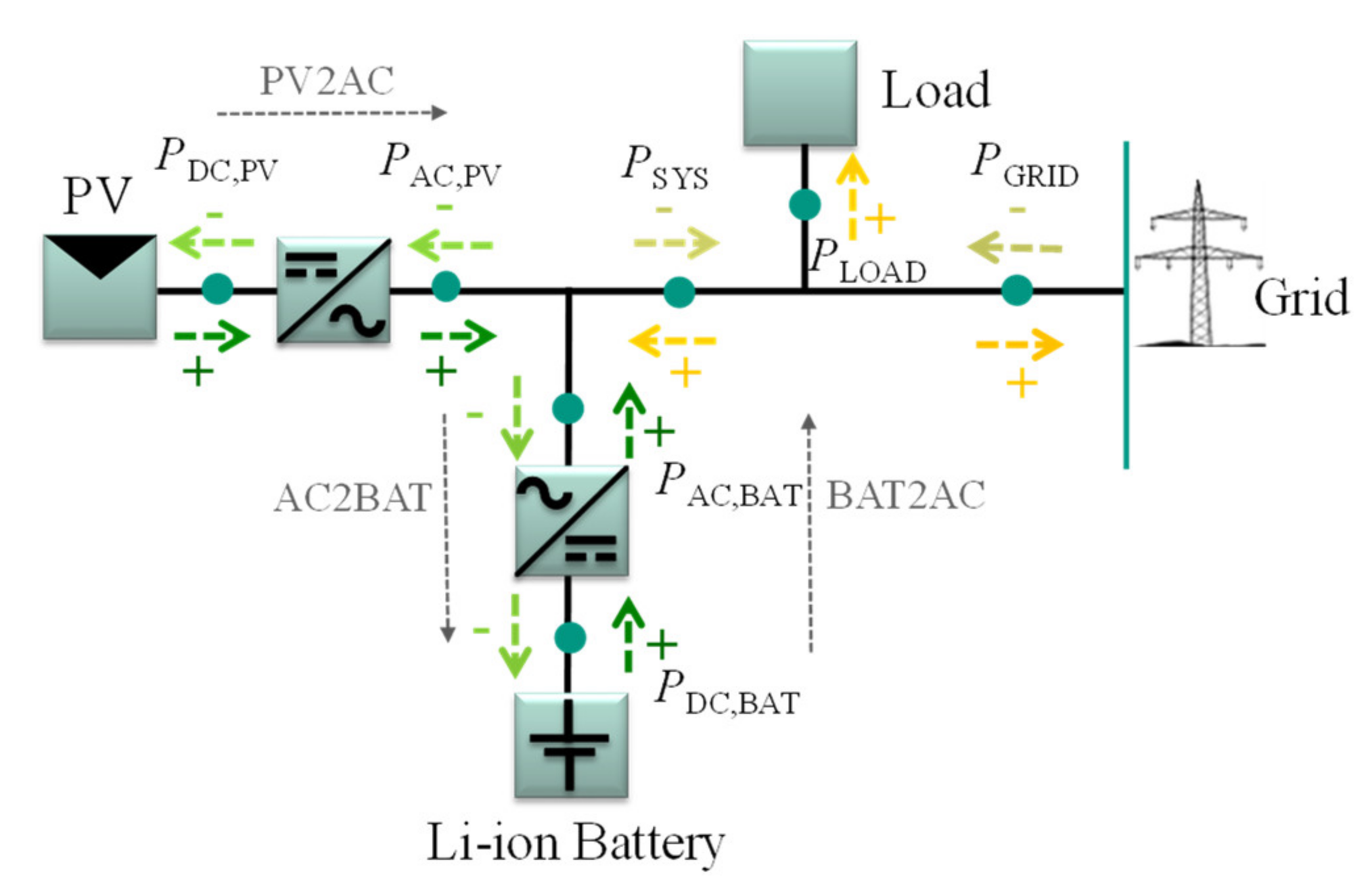
The simulation considers an AC-coupled system, that consists of a battery, a battery inverter, a PV system and a PV inverter (see Figure 1). Figure 1 shows the possible power flows including the corresponding symbols.

3.1. Input Data

3.1.1. PV and Load Data

For the simulation described in this work, real PV data with a sampling rate of 1 Hz from the 1 MW solar-storage park at KIT’s north campus is used. To reduce the simulation time, the resolution is reduced to one minute. Since the reaction time of the systems is not considered in the study, this is sufficient. The PV data were recorded from an array with southerly orientation (0°) and an inclination angle of 30°, which corresponds to a typical house with south-facing pitched roof. It stems from a 10 kWp PV array from 2016 and is scaled to the corresponding PV size used in the simulation. In order to generate appropriate and reproducible load profile data for a single family household (HH) the VDI 4655 standard [61] is used. It describes 10 different types of reference days during the year that make up the synthetic year. The reference household upon which this works’ results are based has an annual electricity consumption of 4213 kWh and corresponds to a five-person household in the VDI 4655 classification. The load profile stems from region 12 of the VDI 4655 profiles, which matches the location where the PV data was sourced (Karlsruhe). The data have a sampling time of one minute.

3.1.2. Battery and Inverter Efficiency and Standby Consumption

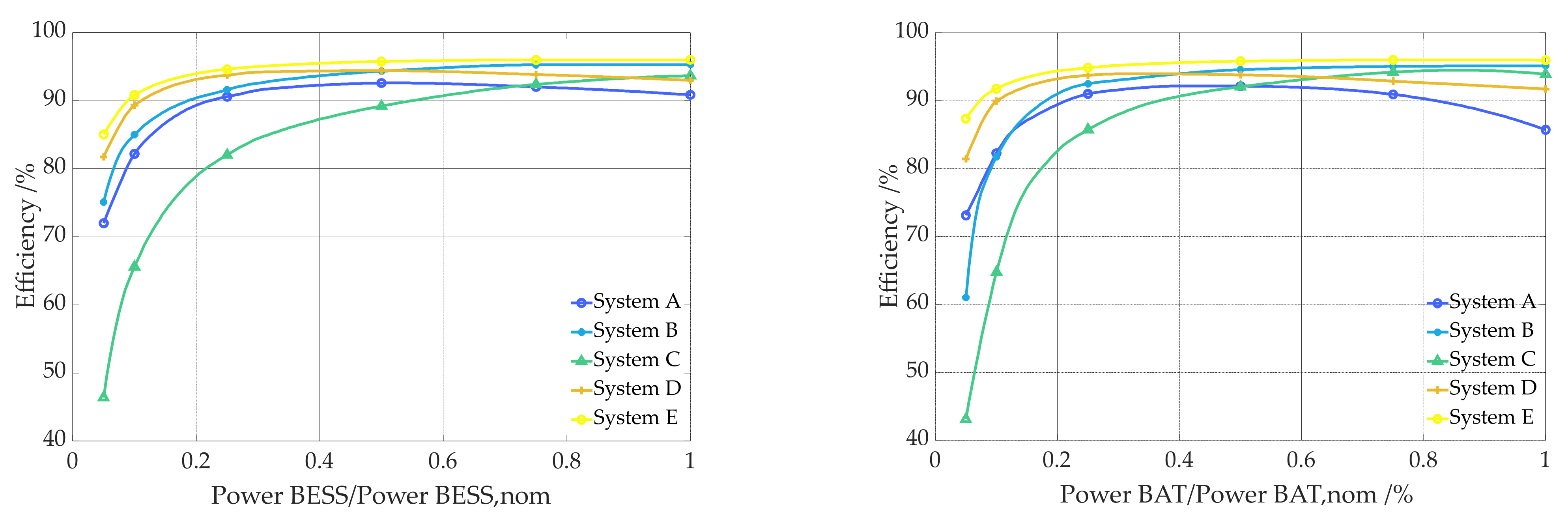
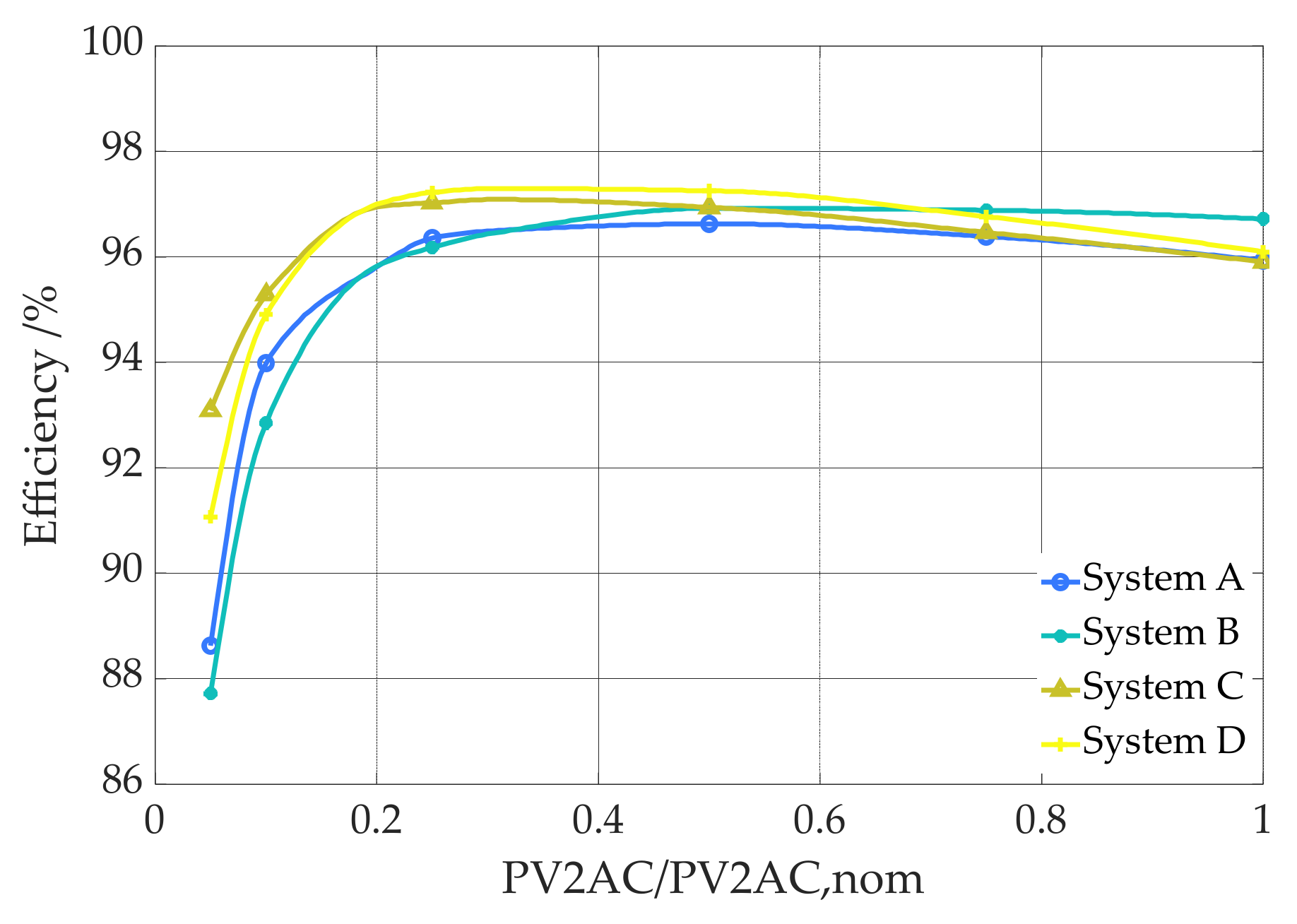
Figure 2 and Figure 3 show efficiency curves of PV storage systems measured in the project “SafetyFirst” and industry projects. The size of the battery inverters of the 5 systems shown here is between 0.8 kW and 6.0 kW. The size of the 4 PV inverters ranges between 2.9 kW and 5.0 kW. The efficiency of the battery inverter of the system D is further considered for the calculation of the reference case (Ref.). For the PV inverter, system D is selected. 3 of the other 4 efficiency curves of the battery inverter (System A, System C and System E) and 1 of the 3 efficiency curves of the PV inverter (System A) are used for the sensitivity analysis. The efficiencies are named in the following according to the different power paths, η_BAT2AC for battery discharging, η_AC2BAT for battery charging and η_PV2AC for the conversion of the DC PV power into AC power.

Table 2. Average pathway efficiencies of the battery inverter.

	Average Pathway Efficiency BAT2AC	Average Pathway Efficiency AC2BAT
System A	89.35	88.68
System C	83.70	85.62
System D (Ref.)	92.50	91.95
System E	94.32	94.66

shows the average pathway efficiencies of the battery inverter of the 4 efficiency curves chosen for the simulation. The average pathway efficiency of the PV inverter is 96.29 for system D (Ref.) and 95.51 for system A. The average pathway efficiencies are calculated as described in the efficiency guideline [62]. The average path efficiency is the arithmetic mean of the efficiencies at the supporting points (0.05; 0.15; 0.25; 0.35; 0.45; 0.55; 0.65; 0.75; 0.85; 0.95) and can be used to compare inverter efficiencies with each other.

$${\eta }_{\mathrm{BAT}}=\sqrt{{\eta }_{\mathrm{BAT},\mathrm{RT}}}$$

(1)

Battery roundtrip efficiencies (η_BAT,RT) for Li-ion home storage systems are usually between 90% and 100%. Many systems are in the range between 95% and 97% [44,63]. For this reason, a value of 96% is selected for the reference case. The efficiency during (η_BAT) charging or discharging can be determined with Equation (1). By simple measurement, only the roundtrip efficiency of storage systems can be determined. How much of this is accounted for by charging and how much by discharging is difficult to determine. For this reason, the same efficiency was assumed for both directions in the present work.

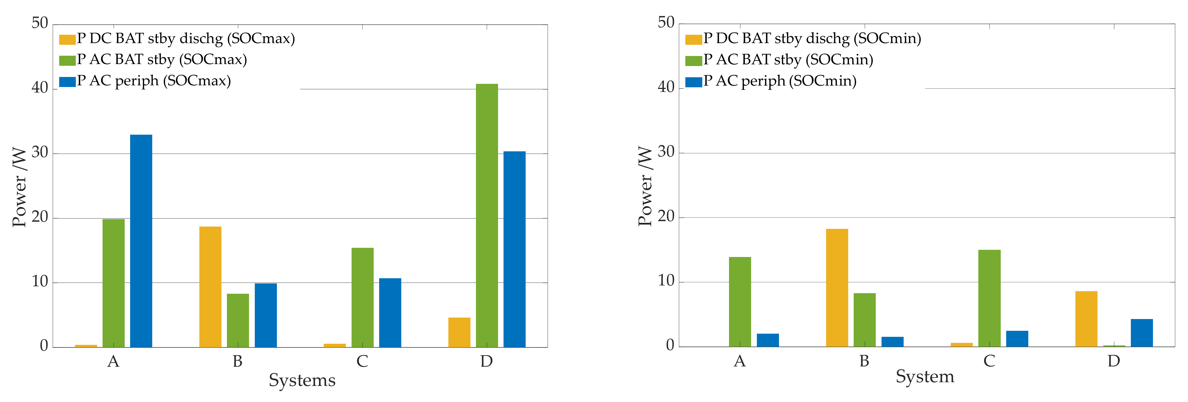
Figure 4 shows measured standby consumption of 4 systems (A to D), which was determined according to the efficiency guidelines. Standby consumption can occur either on the AC side of the battery inverter or on the DC side. Normally, for AC coupled systems, standby consumption can occur on the DC as well as on the AC side when the battery is fully charged or discharged. For the reference case, a standby consumption of 8 W on the DC side and 12 W on the AC side is taken into account. In addition, a peripheral consumption of 8 W is assumed. The values were determined using measured values from 4 AC coupled storage systems with a battery capacity between 2.3 kWh and 4.0 kWh and the mentioned PV and battery inverter sizes in Section 3.1.2 (see Figure 4). While the standby and peripheral consumption at maximum SOC is shown on the left, the standby and peripheral consumption at minimum SOC is shown on the right. The latter are significantly lower. In the simulation, however, only one value is used for both situations (SOC_min and SOC_max). The 8 W peripheral consumption (P_AC,periph) represents a high value of the shown storage systems at minimum SOC and a low value at maximum SOC. Since peripheral consumption always occurs, 8 W of P_AC,periph results in 70.3 kWh of P_AC,periph per year. According to Munzke et al. [44], the P_AC,periph for home storage systems per year is between 13 kWh and 144 kWh. The 8 W assumed here therefore represent a good average value. The DC standby consumption (P_{DC,BAT,stby,dischg}) of the 4 storage systems ranges from 0 W to 19 W, regardless of whether the battery is full or empty. For the references case of the simulation, 8 W are selected. The AC standby consumption (P_AC,BAT,stby) is significantly higher in some systems with a fully charged battery than with a completely discharged battery. In other systems, it is about the same in both cases. Overall, the standby consumption lies between 0 W and 40 W, depending on the system and state. For the simulation, 12 W is selected for the reference case. This leads to standby losses of 60 kWh per year on average in the simulation, which is comparable to the values in Munzke et al. [44].

3.1.3. Chosen Parameters for the Battery, the PV System and the Power Electronic Components

In the simulation, different sized PV systems and batteries as well as different battery inverter sizes are considered. The PV system is varied between 4 kWp and 15 kWp, the battery between 4 kWh and 10 kWh and the battery inverter between 2 kW and 6 kW. The size of the PV inverter always corresponds to the size of the PV system.

3.1.4. Cost

All costs in the simulation include the value-added tax (VAT). The costs for the PV system and the battery depend on the respective component size [64,65,66]. The costs are therefore included in the simulation depending on the size of the PV system and the battery. The invest cost of the PV system can be calculated according to Equation (2) and of the battery according to Equation (3). Equation (2) was derived using the data from Märtel [64].

Table A1. Calculation of the PV system cost per kWp: Costs from Märtel [64] are used as the initial basis for calculating the PV system costs. These can be found in the table in row 1. The costs in the simulation needed only include the costs for the PV system including construction without the inverter. In the simulation the costs for the inverters are 200 €/kW. Thus, the cost of the inverter was deducted from the cost of Märtel. To obtain a simple functional relationship between the PV system size and the PV system cost, the values of 3 kWp and 9 kWp were omitted and the value of 17.5 kWp was corrected to a lower value of 1300 €/kWp. The omitted values are marked in red in the table. The coefficient of determination is 0.9513.

PV System Size/kWp	3	4	5	6	7	8	9	10	12.5	17.5
Cost per kWp without VAT/€ [64]	1.730	1.570	1.530	1.490	1.470	1.370	1.430	1.340	1.240	1.360
Cost per kWp with VAT/€	2.059	1.868	1.821	1.773	1.749	1.630	1.702	1.595	1.476	1.618
Cost of the inverter/€	600	800	1.000	1.200	1.400	1.600	1.800	2.000	2.500	3.500
Total cost of the PV system without inverter/€	5.576	6.673	8.104	9.439	10.845	11.442	13.515	13.946	15.945	24.822
Cost of the PV system per kWp without inverter/€	1.859	1.668	1.621	1.573	1.549	1.430	1.502	1.395	1.276	1.418

in the Appendix A gives an overview of the derivation. For the PV inverter as well as for the battery inverter, a price of 200 €/kW is applied. The battery cost function (Equation (3)) was derived using data from Figgener et al. [66]. The approach can be found in

Table A2. Calculation of the batter cost per kWh: The battery cost function was derived using data from Figgener et al. [66]. These already include the VAT and the inverter costs. The approach is described in the table. In the first step, the data from Figgener et al. was fitted (see Equation (A1)). For all battery sizes between 2 kWh and 10 kWh, the inverter costs are then subtracted from the battery system costs. According to Figgener et al. [66], the average inverter size for storage systems between 5 kWh and 10 kWh is 3.5 kW. The inverter costs are assumed to be 200 €/kW. Thus, for the calculation, for all batteries larger than 5 kWh 700 € was deducted from the storage system costs. For all systems smaller than 5 kWh, only 400 € were deducted for an inverter with a size of 2 kW. From this a functional relationship can be derived, which is represented by Equation (3). The coefficient of determination is 0.9956.

Approach	Data
Data from Figgener et al. [66]	Mean battery size/kWh					3	7.5	12.5	17.5
	Mean battery cost including VAT and the battery inverter/€/kWh					1625	1100	900	825
Derived equation (R2 = 1)	Equation (A1)
Battery size/kWh	2	3	4	5	6	7	8	9	10
Cost of the battery storage system/€	3616	4875	5875	6684	7364	7965	8529	9087	9663
Cost of the battery without an inverter of 2kW/€	1608	1492	1369
Cost of the battery without an inverter of 3.5 kW/€				1197	1111	1038	979	932	896
Derived Equation (3) to calculate battery cost (R2 = 0.9956)

in the Appendix A. The annual battery cost degradation for home storage systems between 5 kWh and 10 kWh was 6.4% per year in 2018 and 2019. Since 2013 the prices have decreased by 55.6%. Since the storage market has developed much further in recent years [1,66], it is assumed that the price reductions will continue in the next few years, but will fall less. Thus, a price reduction of only 3% per year is applied.

Table 3. Input data for electricity cost calculation.

Parameter	Value	Unit
Electricity price [67]	31.89	cent/kWh
Calculation period	20	y
PV system cost (CPV) [64] (see Table A1)	Equation (2)	€/kWp
Battery cost (CBAT) [66] (see Table A2)	Equation (3)	€/kWh
Inverter cost	200	€/kW
Inverter lifetime [22,68,69]	10	y
Annual battery cost degradation	3	%
Price change factor of the battery	0.97
Price change factor of the inverters	1
Annual electricity price increase [4,67]	0.0/1.0	%
Price change factor of the electricity price [4,67]	1.0/1.01
Feed in tariff (March 2021) for PV systems up to 10 kWp	7.92	cent/kWh
Feed in tariff (March 2021) for PV systems between 10 kWp and 40 kWp	7.7	cent/kWh

gives an overview of the input parameters for the cost calculation.

$$C_{\mathrm{PV}}=\left(-0.084·P_{\mathrm{PV},\mathrm{kWp}}{}^3+4.9056·P_{\mathrm{PV},\mathrm{kWp}}{}^2-100.6·P_{\mathrm{PV},\mathrm{kWp}}+2011.2\right)·P_{\mathrm{PV},\mathrm{kWp}}$$

(2)

$$C_{BAT}=\left( 8.7735·E_{\mathrm{CapaBAT}}{}^2-196.38·E_{\mathrm{CapaBAT}}+1984\right)·E_{CapaBAT}$$

(3)

Due to the current low interest rates and the focus of the paper on the influence of technical parameters on the electricity costs, no interest rates are assumed in the paper. In the past, the development of electricity prices was subject to strong fluctuations and it is difficult to predict how they will develop in the future. According to [4,67], the electricity price increase in Germany over the last 8 years was between 1.16% and 1.28% per year on average. In 2021, levies and taxes account for 51% of the household electricity price in Germany. Part of this is the EEG levy due to the German Renewable Energy Sources Act (EEG). The EEG levy is 6.5 cent/kWh in 2021 and will fall to 3.723 cent/kWh in 2022 [70]. Therefore, an increase in electricity costs of only 1% is assumed. In addition, the impact of no cost increase (0.0%) is examined, as electricity prices in Germany are already the highest in Europe. The higher the cost increase with simultaneously very low interest rates, the more economical PV home storage systems are as long as system prices do not rise simultaneously. For the sensitivity analysis, the scenario with a cost increase of 1.0% per year is used.

3.2. Methods

The simulation model is presented below. The simulation of the power flows including the influence of the charging strategy, the economic evaluation and the aging model are discussed in detail.

3.2.1. Simulation of Power Flows Including Different Charging Strategies

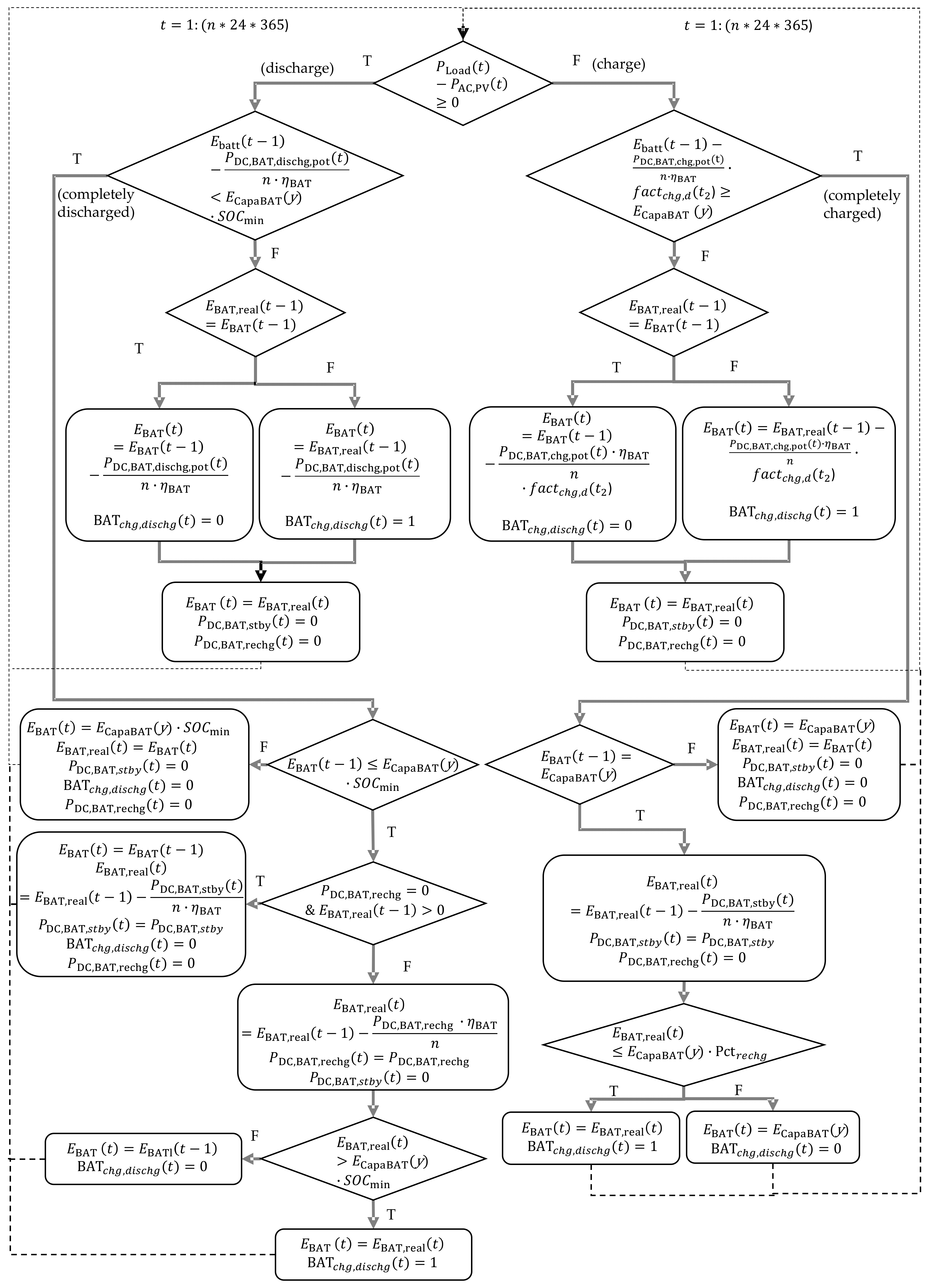
Equations (4)–(16) and Figure 5 and Figure 6 provide a detailed overview of the power flow simulation of the model. In all following calculations, t is the respective simulation step. To account for peripheral consumption, it is added to the load at the beginning of the simulation. Since the efficiencies are considered as a function of power and different efficiency curves are to be considered, PV data from the DC side of the inverter (P_DC,PV) is used for the simulation (see Figure 3). These are converted to AC power (P_AC,PV) using Equation (4). By subtracting the PV power from the load including peripheral consumption (P_Load), potential charging (P_{AC,BAT,chg,pot}) and discharging (P_{AC,BAT,dischg,pot}) powers can be determined (see Equations (5) and (6)). By Equations (7) and (8), these can also be converted to potential battery power (P_{DC,BAT,chg,pot} and P_{DC,BAT,dischg,pot}). It should be noted that the DC power is limited by the selected inverter power (rated power). This applies to both charging and discharging.

$$P_{\mathrm{AC},\mathrm{PV}}\left(t\right)=P_{\mathrm{DC},\mathrm{PV}}\left(t\right) · {\eta }_{\mathrm{PV}2\mathrm{AC}}\left(P_{\mathrm{DC},\mathrm{PV}}\right)$$

(4)

$$P_{\mathrm{AC},\mathrm{BAT},\mathrm{chg},\mathrm{pot}}\left(t\right)=\left\{\begin{array}{l}\left(P_{\mathrm{Load}}\left(t\right)-P_{\mathrm{AC},\mathrm{PV}}\left(t\right)\right)if \left(P_{\mathrm{Load}}\left(t\right)-P_{\mathrm{AC},\mathrm{PV}}\left(t\right)\right)<0 \\ 0if \left(P_{\mathrm{Load}}\left(t\right)-P_{\mathrm{AC},\mathrm{PV}}\left(t\right)\right)>0\end{array}\right\}$$

(5)

$$P_{\mathrm{AC},\mathrm{BAT},\mathrm{dischg},\mathrm{pot}}\left(t\right)=\left\{\begin{array}{l} 0if \left(P_{\mathrm{Load}}\left(t\right)-P_{\mathrm{AC},\mathrm{PV}}\left(t\right)\right)<0 \\ \left(P_{\mathrm{Load}}\left(t\right)-P_{\mathrm{AC},\mathrm{PV}}\left(t\right)\right)if \left(P_{\mathrm{Load}}\left(t\right)-P_{\mathrm{AC},\mathrm{PV}}\left(t\right)\right)>0\end{array}\right\}$$

(6)

$$P_{\mathrm{DC},\mathrm{BAT},\mathrm{chg},\mathrm{pot}}\left(t\right)=P_{\mathrm{AC},\mathrm{BAT},\mathrm{chg},\mathrm{pot}}\left(t\right)· {\eta }_{\mathrm{AC}2\mathrm{BAT}}\left(P_{\mathrm{AC},\mathrm{BAT},\mathrm{chg},\mathrm{pot}}\right)$$

(7)

$$P_{\mathrm{DC},\mathrm{BAT},\mathrm{dischg},\mathrm{pot}}\left(t\right)=\frac{P_{\mathrm{AC},\mathrm{BAT},\mathrm{dischg},\mathrm{pot}}\left(t\right)}{{\eta }_{\mathrm{BAT}2\mathrm{AC}}\left(P_{\mathrm{AC},\mathrm{BAT},\mathrm{dischg},\mathrm{pot}}\right)}$$

(8)

Figure 5 shows a detailed overview of the calculation of the energy charged and discharged in the battery (E_BAT).

DC standby consumption (P_stby,DC,BAT) may occur when the battery is fully charged or discharged. This is the case when a part of the standby consumption of the inverter is covered by the battery and the battery is slightly discharged. To be able to simulate this, the variable E_BAT,real is introduced to avoid immediate recharging of the battery. It refers to the actual state of charge of the battery. In case of a fully charged battery, the following applies. If E_BAT,real has fallen below a certain limit (97.5% SOC) or the battery is discharged in the next time step, E_BAT is set equal to E_BAT,real. The limit is determined by a percentage (Pct_rechg) of the actual total battery capacity left (E_CapaBAT(y)). In the first case the battery is charged again, in the second case the energy discharged from the battery due to standby consumption is taken into account in further operation. To simplify the calculation of the actual charged and discharged power, the additional variable BAT_chg,dischg is introduced. Whenever E_BAT is determined with the help of E_BAT,real, it is set equal to 1. The battery is only discharged to 5% SOC in the simulation during regular operation. This means that the battery is completely discharged at a SOC of 5%. However, it can be further discharged by DC standby losses. As soon as 0% SOC is reached due to standby consumption, the battery is charged from the grid with 500 W (P_DC,BAT,rechg) until a SOC of 5% is reached.

Figure 5. Calculation of the energy stored in the battery and the DC standby consumption—T stands for true and F for false.

Figure 5. Calculation of the energy stored in the battery and the DC standby consumption—T stands for true and F for false.

In this paper, the effect of two different charging strategies is investigated. On the one hand, a charging strategy is investigated that only aims to increase self-consumption of the household. On the other hand, a charging strategy is investigated that aims to increase self-consumption and to operate the battery in such a way that calendar aging is decreased. For the second so-called “intelligent” charging strategy, the variable fact_chg,_d is introduced. This factor is determined for each day (t₂) and depends on the ratio of the battery capacity and its charging efficiency to the PV energy that is not directly consumed by the load (see Equation (9)). When calculating the power charged in the battery, the potential energy available is multiplied by fact_chg,d and thus reduced. Thus, the battery is charged more slowly over the course of the day. This can lead to the battery not being completely full at the end of the day although sufficient energy is available during the day. To prevent this, all days are identified on which fact_chg,d is smaller than 1 and the SOC of the battery does not reach 100%. fact_chg,d is then increased by 0.01 for all days affected by this and the calculation from Figure 5 is repeated. This is done until the battery is fully charged on all days where sufficient energy is available. If the simple charging strategy is used, fact_chg,d in Figure 5 is set to 1.

The actual DC charge (P_DC,BAT,chg) and discharge (P_{DC,BAT,dischg}) power can be determined using BAT_chg,dischg, E_BAT and E_BAT,real. If BAT_chg,dischg is 1, the actual charging power is determined from the difference between E_BAT and E_BAT,real of the previous time step (see Equations (10) and (11)). It must be taken into account that there are situations in which power is required from the battery, but it is already empty and must be recharged from the grid. This must be considered when calculating the actual discharge power. With Equations (12)–(14), the AC charge (P_AC,BAT,chg) and discharge (P_{AC,BAT,dischg}) power as well as the AC recharge power (P_AC,BAT,rechg) of the battery can be determined.

$$fac{t}_{chg,d}\left(t_2\right)=\left\{\begin{array}{c}1 if \frac{E_{CapaBAT}\left(y\right)}{E_{DC,BAT,chg,d}\left(t_2\right)}·{\eta }_{BAT}\ge 1\\ \frac{E_{CapaBAT}\left(y\right)}{E_{DC,BAT,chg,d}\left(t_2\right)}·{\eta }_{BAT}if \frac{E_{CapaBAT}\left(y\right)}{E_{DC,BAT,chg,d}\left(t_2\right)}·{\eta }_{BAT}<1 \end{array}\right\}$$

(9)

$$P_{DC,BAT,chg}\left(t\right)=\left\{\begin{array}{ll}\frac{(E_{BAT}\left(t-1\right)-E_{BAT}\left(t\right))·n}{{\eta }_{BAT}}& if P_{AC,BAT,chg,pot}\left(t\right)<0 \& BA{T}_{chgdischg}\left(t\right)=0\\ \frac{(E_{BAT}\left(t-1\right)-E_{BAT,real}\left(t\right))·n}{{\eta }_{BAT}}& if P_{AC,BAT,chg,pot}\left(t\right)<0 \& BA{T}_{chgdischg}\left(t\right)\ne 0\\ 0& if P_{AC,BAT,chg,pot}\left(t\right)\ge 0 \end{array}\right\}$$

(10)

$$P_{\mathrm{DC},\mathrm{BAT},\mathrm{dischg}}\left(t\right)=\left\{\begin{array}{lll}\frac{(E_{\mathrm{BAT}}\left(t-1\right)-E_{\mathrm{BAT}}\left(t\right))·\mathrm{n}}{{\eta }_{\mathrm{BAT}}}& if P_{\mathrm{AC},\mathrm{BAT},\mathrm{chg},\mathrm{pot}}\left(t\right)\le 0 \&{ \mathrm{BAT}}_{chgdischg}\left(t\right)=0& \& P_{\mathrm{DC},\mathrm{BAT},\mathrm{rechg}}\left(t\right)=0\\ \frac{(E_{\mathrm{BAT}}\left(t-1\right)-E_{\mathrm{BAT},\mathrm{real}}\left(t\right))·\mathrm{n}}{{\eta }_{\mathrm{BAT}}}& if P_{\mathrm{AC},\mathrm{BAT},\mathrm{chg},\mathrm{pot}}\left(t\right)\le 0 \&{ \mathrm{BAT}}_{chgdischg}\left(t\right)\ne 0 & \& P_{\mathrm{DC},\mathrm{BAT},\mathrm{rechg}}\left(t\right)=0\\ 0& if P_{\mathrm{AC},\mathrm{BAT},\mathrm{chg},\mathrm{pot}}\left(t\right)>0 \end{array}\right\}$$

(11)

$$P_{\mathrm{AC},\mathrm{BAT},\mathrm{dischg}}\left(t\right)=P_{\mathrm{DC},\mathrm{BAT},\mathrm{dischg}}\left(t\right)· {\eta }_{\mathrm{BAT}2\mathrm{AC}}\left(P_{\mathrm{DC},\mathrm{BAT},\mathrm{dischg}}\right)$$

(12)

$$P_{\mathrm{AC},\mathrm{BAT},\mathrm{chg}}\left(t\right)=\frac{P_{\mathrm{DC},\mathrm{BAT},\mathrm{chg}}\left(t\right)}{{\eta }_{\mathrm{AC}2\mathrm{BAT}}\left(P_{\mathrm{DC},\mathrm{BAT},\mathrm{chg}}\right)}$$

(13)

$$P_{\mathrm{AC},\mathrm{BAT},\mathrm{rechg}}\left(t\right)=\frac{P_{\mathrm{DC},\mathrm{BAT},\mathrm{rechg}}\left(t\right)}{{\eta }_{\mathrm{AC}2\mathrm{BAT}}\left(P_{\mathrm{DC},\mathrm{BAT},\mathrm{rechg}}\right)}$$

(14)

$$SOC\left(t\right)=\frac{E_{\mathrm{BAT}}\left(t\right)}{E_{\mathrm{CapaBat}}\left(y\right)}$$

(15)

$$P_{\mathrm{AC},\mathrm{BAT},\mathrm{stby}}\left(t\right)=\left\{\begin{array}{ll}{P}_{\mathrm{AC},\mathrm{BAT},\mathrm{stby}}& if \left(SOC \left(t\right)\le SO{C}_{min} \& P_{\mathrm{DC},\mathrm{BAT}}\left(t\right)=0 \& P_{\mathrm{DC},\mathrm{BAT},\mathrm{rechg}}\left(t\right)=0\right) \left|\right| SOC \left(t\right)=100\\ 0 & if (SOC \left(t\right)>SO{C}_{min} \left|\left| P_{\mathrm{DC},\mathrm{BAT}}\left(t\right)\ne 0 \right|\right| P_{\mathrm{DC},\mathrm{BAT},\mathrm{rechg}}\left(t\right)\ne 0) \left|\right| SOC \left(t\right)=100\end{array}\right\}$$

(16)

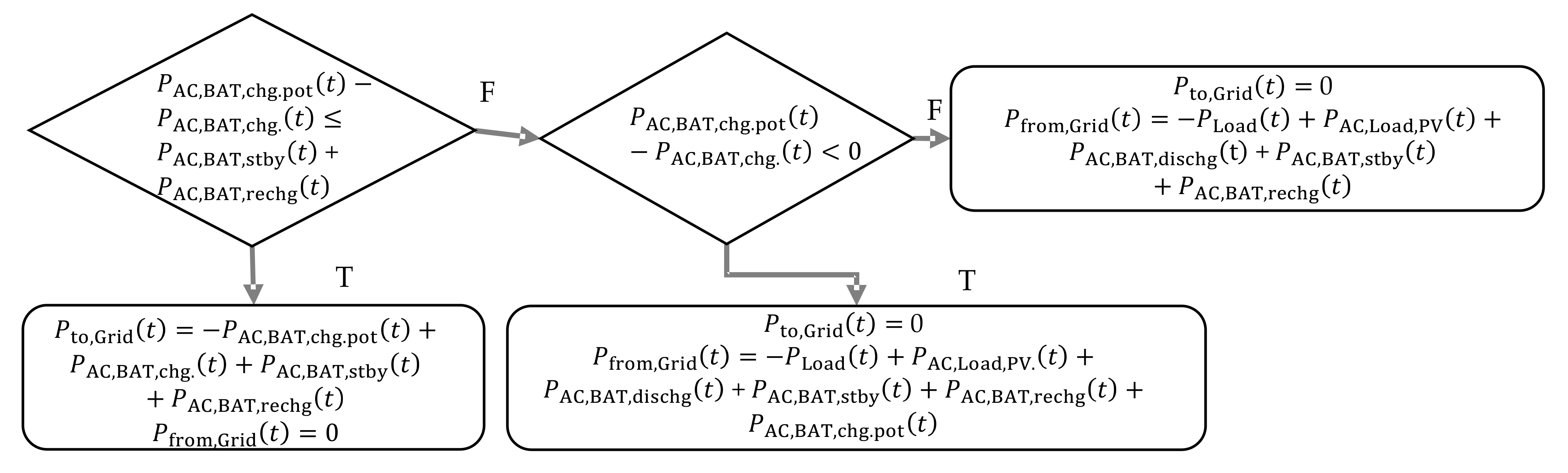
Figure 6. Calculation of the grid consumption and the grid feed-in—T stands for true and F for false.

Figure 6. Calculation of the grid consumption and the grid feed-in—T stands for true and F for false.

AC standby power can either occur when the battery is empty or when it is full [44]. The standby power can be determined with Equation (16) using the SOC of the battery and the determined DC battery power. The latter needs to be considered, as the battery’s SOC can be lower than the minimum SOC and the battery is charged or recharged.

To determine the system operator’s energy costs, both the amount of energy fed into the grid and the amount of energy drawn from the grid are required. Figure 6 shows how the corresponding power can be calculated.

3.2.2. Aging Model

As mentioned, the simulation takes into account both the degradation of the PV system and the aging of the battery. According to Kiefer et al. [71], the degradation of PV systems is around 0.15% per year. Therefore, this value is chosen for the simulation. Consequently, the power of the PV plant decreases every year by 0.15% of the initially installed generator power. For the sensitivity analysis a degradation of 0.5% is chosen.

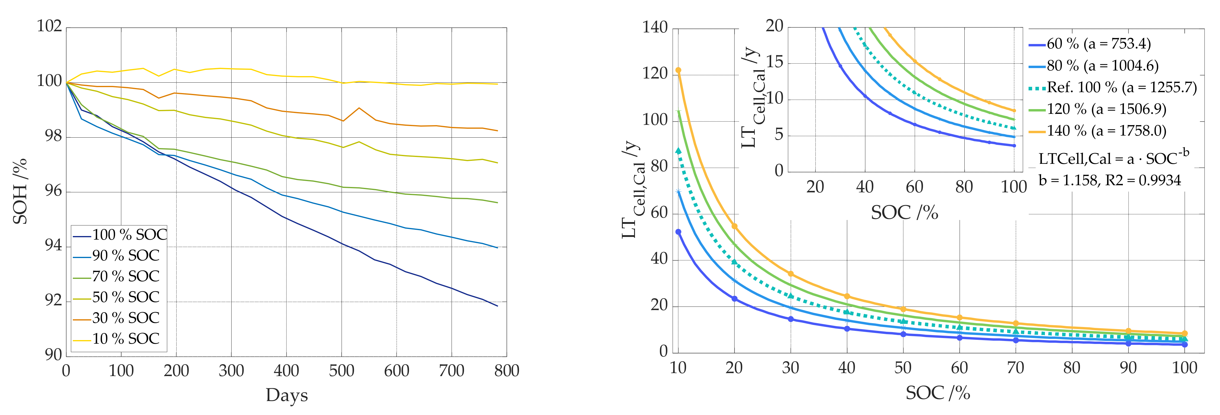
Cell measurement data from a 53 Ah NMC-based pouch cells was used for the battery aging model. Aging of Li-ion cells occurs through cyclic aging [72] on the one hand and through calendar aging, which is primarily dependent on temperature and SOC [73,74], on the other hand. For the calendar aging model, calendric aging tests were performed at different SOCs at 25 °C. The pouch cells were stored in a climatized room at 25 °C (23.8–25.0 °C actual temperature) at the respective SoC (10, 30, 50, 70, 90, 100%). Every 28 days the cells were connected to a Basytec HPS potentiostat for measurement of the remaining cell capacity. Therefore, at first cells were fully discharged to 3.0 V applying a C-rate of 1C. Subsequently, they were charged with 1C to 4.2 V, followed by a CV-phase until I < C/20 to guarantee complete charging. The remaining discharge capacity was determined in the following discharge half cycle applying 1C. For further storage of the cells, each cell was then charged to the according storage SOC by charge with 1C until Ah = Ah (SoC) based on the newly determined full discharge capacity. All experiments were duplicated. Since only low loads are generally applied in stationary home storage systems and the cells therefore show no significant heat evolution, the data at 25 °C were used for this study and the temperature dependence of the calendar aging is neglected. The results of the measurements can be found in Figure 7 left panel. Shown is the average of the two measurements per SOC. The results can be used to calculate the theoretical lifetime (LT_Cell,Cal) in years per SOC. This is shown as a dashed line in Figure 7, right panel, as a function of the SOC. The following functional relationship between life time in years and SOC can be derived by fitting from the measurement (see Equation (17)).

Aging is calculated per year in the simulation. The SOC profile calculated with Equations (15) and (17) are used to determine the calendar aging for each time step. The calendric aging per time step is then summed up to the calendric aging per year (A_Cal(y)) (see Equation (18)). A_Cal(y) represents the percentage that the battery has degraded due to calendar aging in a given year. 100% degradation corresponds to EOL of the battery with a SOH of 80%.

$$L{T}_{\mathrm{Cell},\mathrm{Cal}}=1255.7·SO{C}^{-1.158}$$

(17)

$$A_{\mathrm{Cal}}\left(y\right)={{\displaystyle \sum }}_{t=1}^{365·24·n}\frac{\frac{1}{365·24·n}}{L{T}_{Cell,Cal} \left(t\right)}$$

(18)

In the sensitivity analysis, the influence of aging on economic efficiency is analyzed in this paper. The two upper and lower lines in Figure 7 right panel represent a 20% and 40% higher and lower calendar aging, respectively. For this purpose, the original values at 10, 30, 50, 70, 90 and 100% were multiplied by 0.6, 0.8, 1.2 and 1.4, respectively. Values larger than 20 years are only theoretical values needed for the calculation of the degradation at low SOCs. In the field material degradation and/or leaks have to be considered, such as moisture will enter the cell over time and cause further degradation.

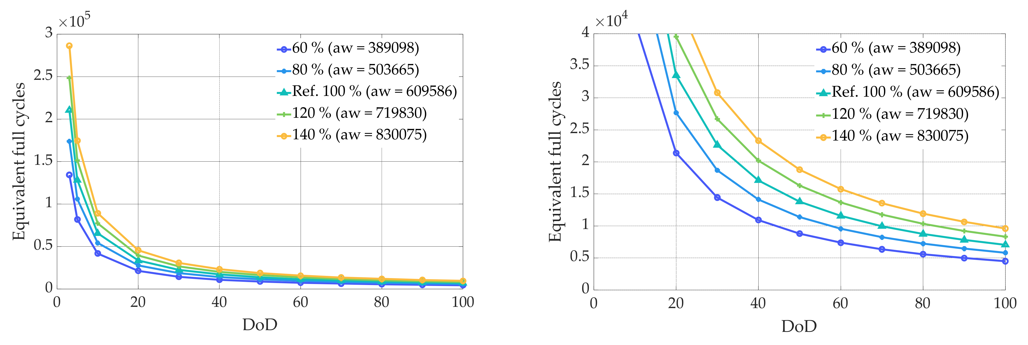
For cyclic aging, 1P1P measurements at 100% DoD at 25 °C were performed using the corresponding cell. 1P1P means that the 193.45 Wh cell under investigation is charged and discharged with 193.45 W. The cycle life of the corresponding cell is 7050 cycles until the remaining capacity of the cell reaches 80%. This represents the average value of two cells. The dependence of cycle life on DoD can be represented by the Wöhler curve [75]. In order to take this effect into account in the present work, the Wöhler curve of an NMC cell [3] from the literature was used and scaled so that 7050 cycles are achieved at 100% DoD. During cycling, the cell ages mainly at the graphite anode due to volume change, resulting in irreversible loss of cyclable lithium ions [73,76,77,78,79]. A high cycle life is usually achieved by suitable additives and/or a better formation procedure [79,80,81,82]. In principle, however, the aging processes are similar, regardless of how cycle-stable the cells are. Therefore, it is assumed that in the absence of measurement data, a curve from the literature can also be used and scaled. The scaled Wöhler curves are represented in Figure 8. The curve in the middle represents the reference curve (Ref. 100%). 60% and 80% represent 40% and 20% higher cyclic aging than the reference case, and 120% and 140% represent 20% and 40% lower cyclic aging. The Wöhler curve can be described with an exponential function. (see Equation (19)), where N(ΔSOC) represents the number of equivalent full cycles [3,83]. To determine the number of cycles with respect to ΔSOC the rainflow algorithm is used. Cyclic aging depends not only on DoD but also on average SOC. However, no reliable data are available for this. For this reason, this dependence is neglected and will be a part of future work. As calendric aging, cyclic aging is also determined per year (see Equation (20)). ni_Cycl represents a factor that can be 1 or 0.5, depending on whether the corresponding cycle is a half or full cycle and Cycl the number of cycles per year. A_Cycl(y) represents the percentage that the battery has degraded due to cyclic aging in a given year. 100% degradation corresponds to EOL of the battery with a SOH of 80%. The total aging results from the sum of the calendar aging and the cyclic aging (see Equation (21)). It is important that the calendar aging was previously subtracted from the cyclic aging. As mentioned, a value of 80% SOH is considered as the end of life criterion. The SOH at the end of a year can be calculated with Equation (22).

$$N\left(\Delta SOC\right)=a_w·\Delta SO{C}^{b_w}$$

(19)

$$A_{Cycl}\left(y\right)={{\displaystyle \sum }}_{n_{Cycl}=1}^{Cycl}\frac{1}{N\left(\Delta SOC, n_{Cycl}\right)·n{i}_{Cycl}\left(n_{Cycl}\right)}$$

(20)

$$E_{\mathrm{CapaBAT}}\left(y+1\right)=E_{\mathrm{CapaBAT}}\left(y\right)-\left(A_{Cycl}\left(y\right)+A_{Cal}\left(y\right)\right)·0.2·E_{\mathrm{CapaBAT}}$$

(21)

$$SOH\left(y+1\right)=SOH\left(y\right)-\left(0.2·\left(A_{Cycl}\left(y\right)+A_{Cal}\left(y\right)\right)·100\right)$$

(22)

3.2.3. Economic Evaluation

To calculate the economic efficiency, the annuity method [84] is used and the different variations are compared on the basis of the levelized cost of energy (LCOE). The annuity of the capital related costs (A_N,C,X) for the PV system, the power electronics and the battery can be determined using Equations (23)–(27). In this context, X as a variable stands for one of the mentioned components. For the PV system, a lifetime of 20 years is assumed, which corresponds to the usual depreciation period for PV systems. Since the simulation period T also corresponds to 20 years, no calculation of replacement investments and residual value is necessary. For the inverters it is assumed that they have to be replaced after 10 years. Thus, the cash values (A_i,PE) of the replacement investments can be determined with Equation (24), where i represents the number of the replacement and T_N the number of years of the depreciation period. The replacement of the battery depends on the aging of the battery. The degree of aging depends on various factors, such as the battery size, the load profile and the PV system. How to determine the aging of the battery and when to replace it is described in Section 3.2.2. Equation (25) can be used to calculate the cash value of the replacement investment of the battery, and Equation (26) to calculate the residual value. y_n,BAT,repl represents the year in which the respective investment takes place. The residual value of the battery depends on the remaining capacity (E_Capa,BAT(y)) at the end of the simulation. r in the equations stands for the respective price change factor. Interest rates can be taken into account in the calculation via the interest factor q. Although the load and PV curves in the simulation remain the same each year, the amount of electricity fed into (E_to,Grid) or taken from the grid (E_from,Grid) changes over the years. This is due to battery aging and degradation of the PV system. The annuity of the annual remuneration for electricity fed into the grid (A_N,R) and the electricity costs of the electricity purchased from the grid (A_N,EC) can be determined using Equations (28) and (29). Where y stands for the respective year in which the costs or the remuneration occur. In the given case, the annuity of the total annual payments (A_N) is the difference between A_N,R and the sum of the capital-related annuities and A_N,EC (see Equation (30). To calculate the cost per kWh (C_E,total), the annuity is divided by the energy consumed per year (E_Load,y) (see Equation (31)). The costs (C_E,total,ref) can be compared with reference costs that would arise if no plant is built and the entire electricity demand would need to be covered by the grid (see Equation (32)).

$$A_{\mathrm{N},\mathrm{C},\mathrm{X}}=\left(A_{0,\mathrm{X}}+A_{1,\mathrm{X}}+A_{2,\mathrm{X}}+\dots .A_{m,\mathrm{X}}-R_{\mathrm{V},\mathrm{X}}\right)·a$$

(23)

$$A_{i,\mathrm{PE}}=A_{0,\mathrm{PE}}·\frac{r_{\mathrm{PE}}{}^{i_{\mathrm{PE}}·T_{\mathrm{N},\mathrm{PE}}}}{q^{i_{\mathrm{PE}}·T_{\mathrm{N},\mathrm{PE}}}}$$

(24)

$$A_{i,\mathrm{BAT}}=A_{0,\mathrm{BAT}}·\frac{r_{\mathrm{BAT}}{}^{y_{i,\mathrm{BAT},\mathrm{repl}}}}{q^{y_{i,\mathrm{BAT},\mathrm{repl}}}}$$

(25)

$$R_{\mathrm{V},\mathrm{BAT}}=A_{0,\mathrm{BAT}}·r_{\mathrm{BAT}}{}^{y_{i,\mathrm{BAT},\mathrm{repl}}}·\frac{\left(\frac{E_{\mathrm{CapaBAT}}\left(T+1\right)}{E_{\mathrm{CapaBAT}}}-0.8\right)}{0.2}·\frac{1}{q^T}$$

(26)

$$a=\frac{q-1}{1-q^{-T}}$$

(27)

$$A_{\mathrm{N},\mathrm{R}}={{\displaystyle \sum }}_{y=1}^T{E}_{\mathrm{to},\mathrm{Grid}}\left(y\right)·r_{E_{\mathrm{to},\mathrm{Grid}}}{}^y·\frac{1}{q^y}$$

(28)

$$A_{\mathrm{N},\mathrm{EC}}={{\displaystyle \sum }}_{y=1}^T{E}_{\mathrm{from},\mathrm{Grid}}\left(y\right)·r_{E_{\mathrm{from},\mathrm{Grid}}}{}^y·\frac{1}{q^y}$$

(29)

$$A_{\mathrm{N}}=A_{\mathrm{N},\mathrm{R}}-A_{\mathrm{N},\mathrm{EC}}-\left(A_{\mathrm{N},\mathrm{C},\mathrm{PV}}+A_{\mathrm{N},\mathrm{C},\mathrm{BAT}}+A_{\mathrm{N},\mathrm{C},\mathrm{DCACPV}}+A_{\mathrm{N},\mathrm{C},\mathrm{DCACBAT}}\right)$$

(30)

$$C_{E,\mathrm{total}}=\frac{A_{\mathrm{N}}}{E_{\mathrm{Load},\mathrm{y}}}$$

(31)

$$C_{E,\mathrm{ref}}=\frac{A_{\mathrm{N},\mathrm{EC},\mathrm{ref}}}{E_{\mathrm{Load},\mathrm{y}}}$$

(32)

Due to the EEG, either only 70% of the generator power may be fed into the grid or a ripple control receiver must be installed. With the latter, the PV system can be regulated down by the grid operator in the event of grid overload. The costs for a ripple control receiver are very variable and range between 200 € and 500 € [85]. For smaller PV systems with an installed power below 10 kWp, the feed-in limitation is usually cheaper than the installation of a ripple control receiver. In the simulation, this is solved as follows. If throttling the feed-in power is cheaper, this is chosen for the corresponding variation. In the other case, the installation of a ripple control receiver is selected. The assumed costs for a ripple control receiver in the simulation are 450 €.

3.3. Parameters Studied

Table 4. Technical parameters studied.

Parameter	Variation		Reference Case	Variation
	V1	V2	Ref.	V3	V4
Battery inverter efficiency	System C	System A	System D	System E	-
PV inverter efficiency	System A	-	System D	-	-
Battery efficiency	92%	94%	96%	98%	99%
Standby consumption AC	0 W	6 W	12 W	18 W	24 W
Standby consumption DC	0 W	4 W	8 W	12 W	16 W
Consumption of peripheral components	0 W	4 W	8 W	12 W	16 W
Charging strategy	-	-	Simple strategy only to enhance self-consumption	-	Strategy to enhance self-consumption and to reduce battery aging
Battery calendar aging	60%	80%	100%	120%	140%
Battery cyclic aging	60%	80%	100%	120%	140%
PV degradation per year	-	-	0.15%	0.32%	0.5%

gives an overview of the parameters studied and which are used in the sensitivity analysis. Four different variations are examined for most of the parameters mentioned. One of the parameters is varied in each simulation run. V1 to V4 refer to the respective variation of each parameter.

4. Results

4.1. System Design Single Family Household

4.1.1. Effects of the Size of the PV Field, the Battery and the Battery Inverter

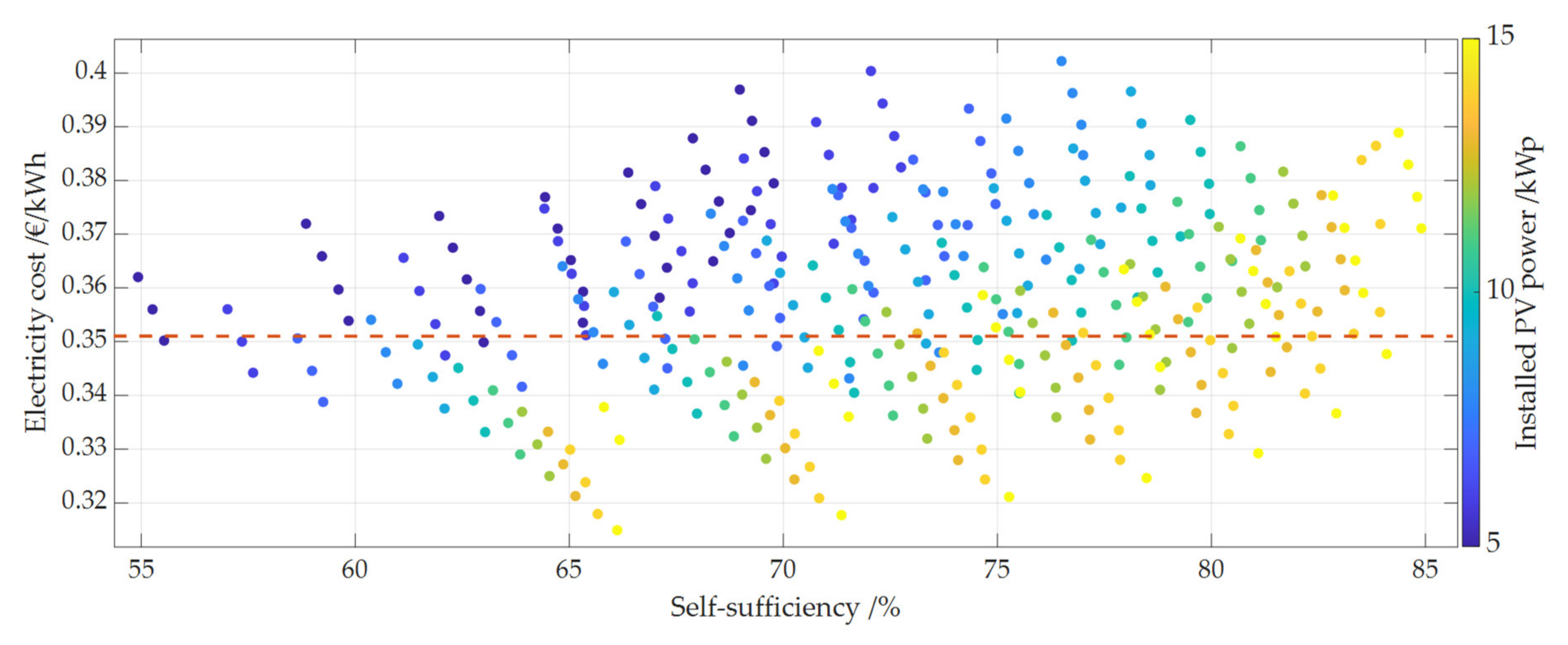
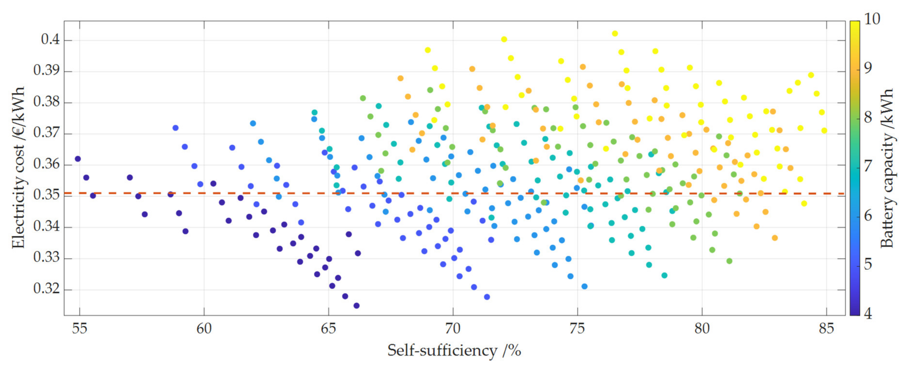
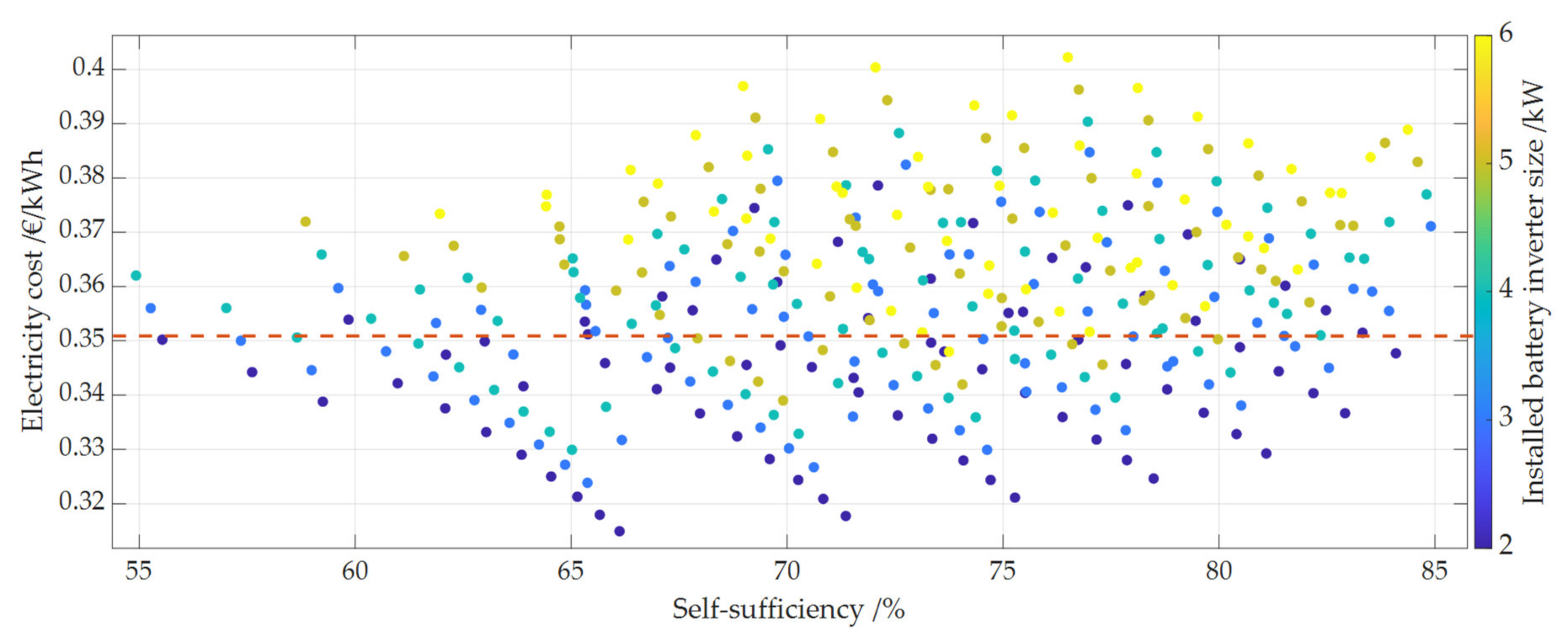
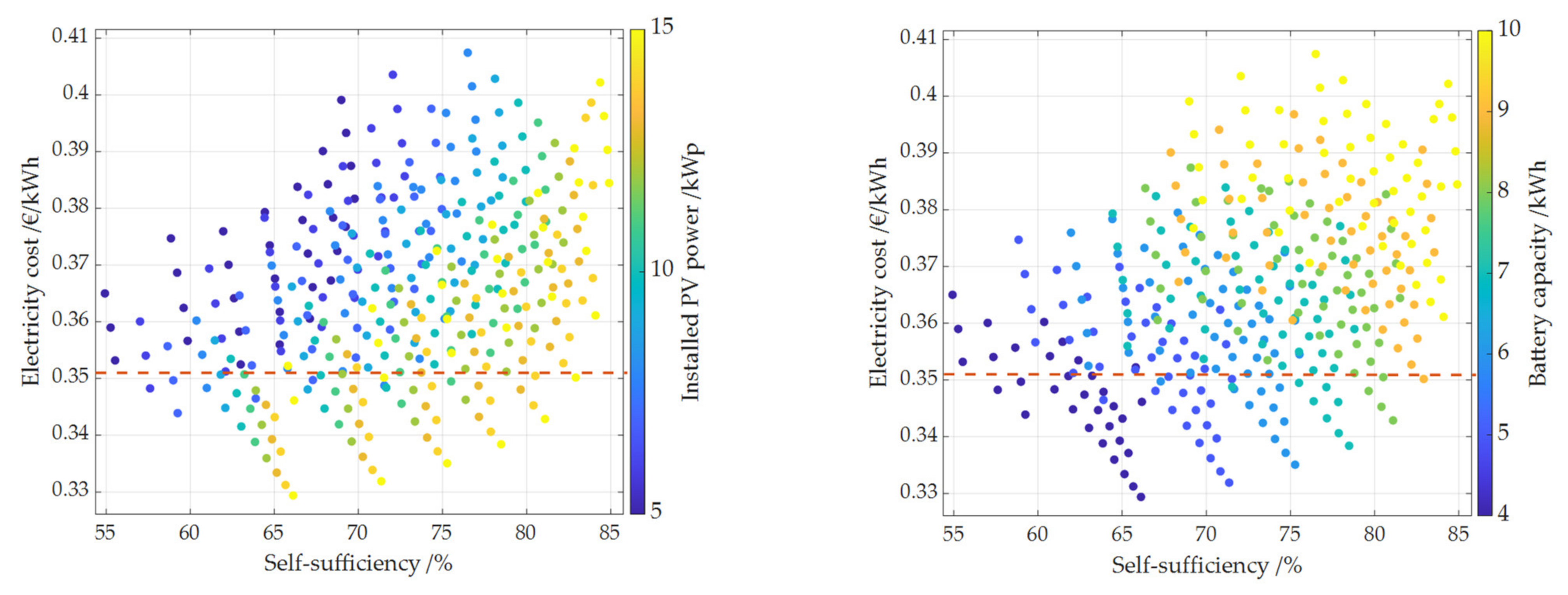
Figure 9, Figure 10 and Figure 11 show the dependence of electricity costs of the reference case on the degree of self-sufficiency. The size of the installed PV system, the battery capacity and the battery inverter size are in color. The electricity costs include all costs to cover the complete electricity demand of the household (see Equation (30)). This includes both the costs for the electricity generated by the PV storage system and for the electricity purchased from the grid to cover the electricity demand that cannot be covered by the PV storage system.

Larger PV systems lead to significantly lower electricity costs than the small ones. At the same time, smaller batteries result in lower electricity costs than larger ones. Although the cost of batteries per kWh installed decreases the larger the battery, the cost of electricity per kWh installed still increases under current conditions. Exemplary this is shown in

Table 5. Example of cost increase due to installation of larger batteries.

Battery Capacity/kWh	4	5	6	7	8	9	10
PV system size/kWp	15	15	15	15	15	15	15
Electricity cost €/kWh	0.3150	0.3178	0.3211	0.3246	0.3293	0.3367	0.3477
Annual cost/€	1327	1339	1353	1368	1387	1418	1465
Total cost 20 years/€	26,540	26,776	27,060	27,356	27,744	28,368	29,297
PV system size/kWp	10	10	10	10	10	10	10
Electricity cost €/kWh	0.3332	0.3366	0.3405	0.3447	0.3502	0.3582	0.3696
Annual cost/€	1404	1418	1435	1452	1475	1509	1557
Total cost 20 years/€	28,076	28,365	28,691	29,050	29,509	30,185	31,143

for a PV system with 15 kWp and 10 kWp. The best combination for the reference case is a PV system of 15 kWp, a battery capacity of 4 kWh and a battery inverter of 2 kWp. For the reference case (see Figure 11) as well as during a first sensitivity analysis of the technical parameters on electricity costs, it turned out that for the assumed load curve and the current framework conditions, the 2 kW battery inverter always represents the most favorable battery inverter size. Inverter sizes of 2 kW, 3 kW, 4 kW, 5 kW and 6 kW were investigated. The load profile has a large effect on this. In most households that have neither an electric car nor a heat pump, about 70 to 80% of the energy is discharged at a power lower than 2 kW [44,63]. In addition, the combination of a larger PV system and a small battery means that the latter can be fully charged during the day even with a small battery inverter, since there is plenty of PV surplus power available. Another advantage is that the battery spends less time at high SOC and therefore ages less. For this reason, the following sensitivity analysis was only performed with 2 kW battery inverters.

Figure 9. Electricity costs as a function of self-sufficiency, the size of the PV system is shown in color. The simulation is based on an annual electricity price increase of 1%.

Figure 9. Electricity costs as a function of self-sufficiency, the size of the PV system is shown in color. The simulation is based on an annual electricity price increase of 1%.

Figure 10. Electricity costs as a function of self-sufficiency, the capacity of the battery is shown in color. The simulation is based on an annual electricity price increase of 1%.

Figure 10. Electricity costs as a function of self-sufficiency, the capacity of the battery is shown in color. The simulation is based on an annual electricity price increase of 1%.

Figure 11. Electricity costs as a function of self-sufficiency, the size of the battery inverter is shown in color. The simulation is based on an annual electricity price increase of 1%.

Figure 11. Electricity costs as a function of self-sufficiency, the size of the battery inverter is shown in color. The simulation is based on an annual electricity price increase of 1%.

The orange line in Figure 9, Figure 10, Figure 11, Figure 12 and Figure 13 represents the grid electricity purchase price in each case. Assuming a cost increase of 1% per year, the average price over the next 20 years will be 35.11 cent/kWh.

4.1.2. Effects of Electricity Price Increase and Feed-In Tariff Decrease

Figure 12. Electricity costs as a function of self-sufficiency. The size of the PV system is shown in color in the left panel and the capacity of the battery is shown in color in the right panel. The simulation is based on an annual electricity price increase of 0%.

Figure 12. Electricity costs as a function of self-sufficiency. The size of the PV system is shown in color in the left panel and the capacity of the battery is shown in color in the right panel. The simulation is based on an annual electricity price increase of 0%.

Figure 13. Electricity costs as a function of self-sufficiency. The size of the PV system is shown in color left panel and the capacity of the battery is shown in color in the right panel. The simulation is based on an annual electricity price increase of 1% and the expected feed-in tariff in June 2021 (7.47 cent/kWh for PV systems up to 10 kWp and 7.25 cent/kWh for PV systems up to 40 kWp).

Figure 13. Electricity costs as a function of self-sufficiency. The size of the PV system is shown in color left panel and the capacity of the battery is shown in color in the right panel. The simulation is based on an annual electricity price increase of 1% and the expected feed-in tariff in June 2021 (7.47 cent/kWh for PV systems up to 10 kWp and 7.25 cent/kWh for PV systems up to 40 kWp).

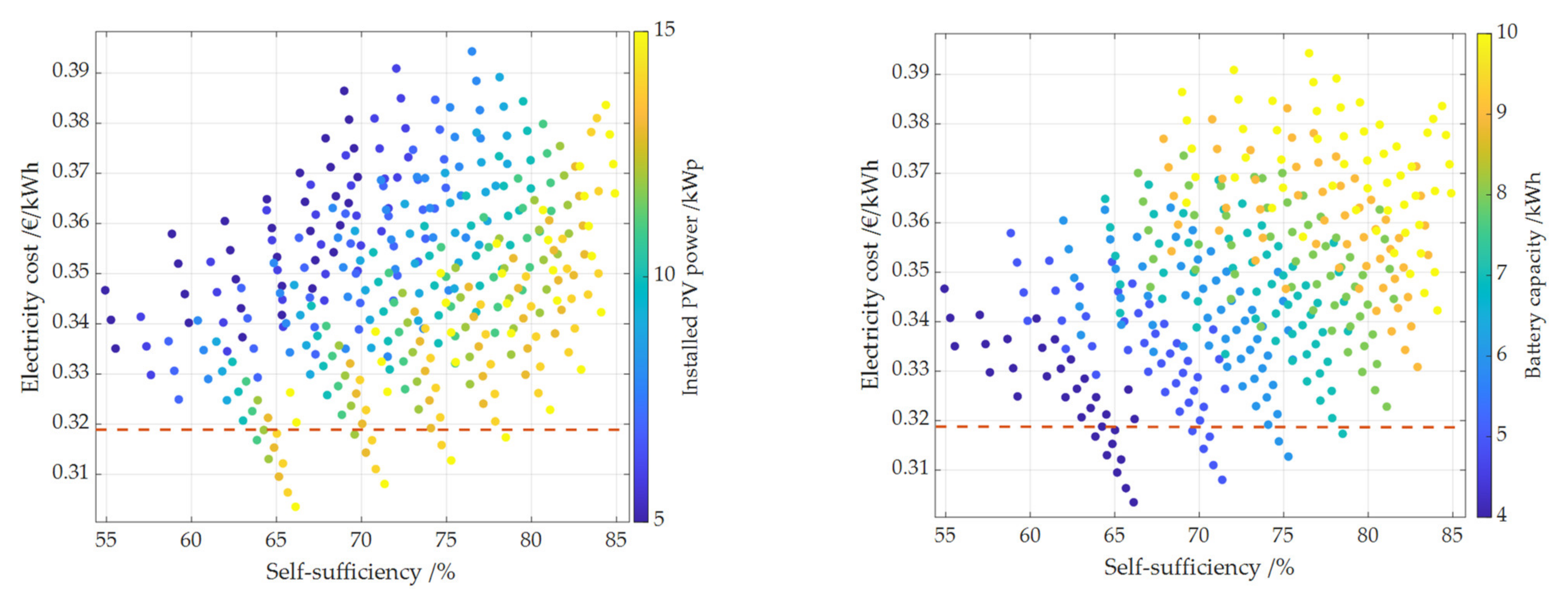
It is very difficult to make a statement about which systems are worthwhile in the longer term, as this depends strongly on the economic framework conditions. If the cost of electricity does not rise or the feed-in tariff falls, far fewer systems will be economical (see Figure 12 and Figure 13). Without electricity cost increase, the cost of electricity purchased from the grid is at the current electricity price of 0.3189 €/kWh. 0% increase in electricity prices would already make PV systems of less than 11 kWp with a battery of at least 4 kWh battery capacity no longer competitive compared to grid consumption. The same applies to all combinations with a battery larger than 7 kWh.

Due to the current new PV installation of 400–600 kWp [86] per month (in 2021), the feed-in tariff is decreasing by 1.4% per month in Germany. This has a strong impact on the profitability of future plants. The effects of the decrease in the feed-in tariff are shown in Figure 13 for the expected feed-in tariff for June 2021. The changes in the economic framework conditions mentioned here do not represent a complete sensitivity analysis of economic parameters on the economic viability of PV storage systems. However, they should give an indication to be able to better interpret the change in economic efficiency due to technical parameters. The expected feed-in tariff for June 2021 would already make PV systems of less than 6 kWp no longer competitive compared to grid consumption. The same applies to all combinations with a battery larger than 9 kWh.

Various studies in the literature show a similar dependence of the economic efficiency on the feed-in tariff and grid electricity prices [13,23,27]. However, in the contributions quite favorable battery prices (500–600 €/kWh) are considered, which have not yet been reached.

4.2. Sensitivity Analysis of Technical Parameters on Electricity Costs of the System Operator

The following section examines the influence of the various technical parameters given in Table 4 on system sizing and electricity costs. In each case, the influence of the battery and the PV system size is examined in detail. As mentioned, the cost of electricity purchased from the grid for the reference case is 31.89 cent/kWh. With a cost increase of 1%, this leads to average cost of 35.11 cent/kWh over 20 years.

4.2.1. Effects of the Efficiency of Power Electronics

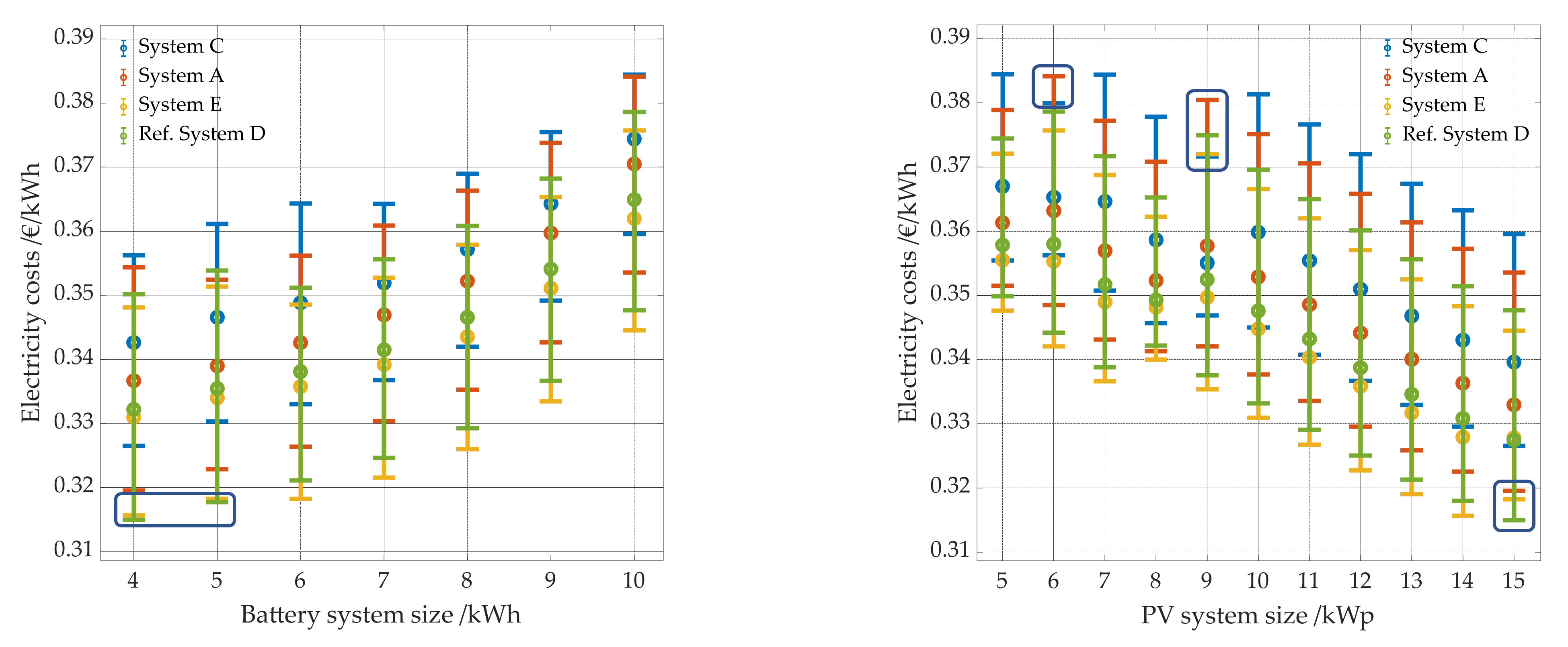
Figure 14 shows the electricity costs per kWh and Figure 15 the annual electricity cost depending on the PV system size (right panel) and the battery system size (left panel). The point in the middle of the error bars represents the average value of all variations with the respective PV system size or battery system size. For example, for 5 kWp PV, this includes all combinations with a 5 kWp PV system and a battery between 4 kWh and 10 kWh. The error bars show the lowest or highest costs for the combinations. Also shown is the dependence of the costs on the efficiency curve used for the battery inverter. For the sensitivity analysis, all PV battery combinations were simulated with different efficiency curves of the battery inverter of systems C, A, E and D (see Figure 2). The average pathway efficiencies for the different efficiency curves are shown in Table 2. The reference case is shown in green. It is interesting to note that it is not always the system with the best performing inverter that results in the lowest total cost. The lowest cost of the reference case with the second most efficient inverter (Ref. System D) with a 4 kWh battery is 31.49 cent/kWh, with a 5 kWh battery it is 31.77 cent/kWh. In contrast, the lowest cost of a system with the most efficient inverter (System E) is 31.82 cent/kWh with a 4 kWh battery and 31.56 cent/kWh with a 5 kWh battery.

The reason for this is that the more efficient inverter charges the battery faster and discharges it slower, since there are fewer losses due to the power electronics during charging and discharging. On the one hand, this means the battery sees more cycles, and on the other hand, it stays in a higher state of charge for a longer period of time, which leads to more battery aging. The battery is better utilized, but must be replaced sooner, which leads to higher costs. From a battery size of 6 kWh, this is less significant. A comparison of the change in energy costs due to the use of a different efficiency curve in the simulation makes the effect even clearer (see Figure 16 left panel). Especially at 4 kWh and 5 kWh, but partly still at 6 kWh and 7 kWh, the costs increase for some PV systems battery storage combinations by using the efficiency curve E instead of the reference curve D in the simulation. The PV system battery combinations where this occurs consist of a 15 kWp PV system and a 4 kWh and 5 kWh battery as well as an 8 kWp PV system and a 6 kWh and 7 kWh battery. The most economic PV system battery storage combination of the simulation with inverter curve E consists of a 14 kWp PV system and a 4 kWh battery and not, as with the other three inverter curves, of a 15 kWp PV system and a 4 kWh battery. Thus, the phenomenon can also be seen in Figure 14 (right window). Similar effects occur with regard to the most expensive PV system battery combination with a PV system size of 6 kWp and 9 kWp and the two lower inverter efficiency curves.

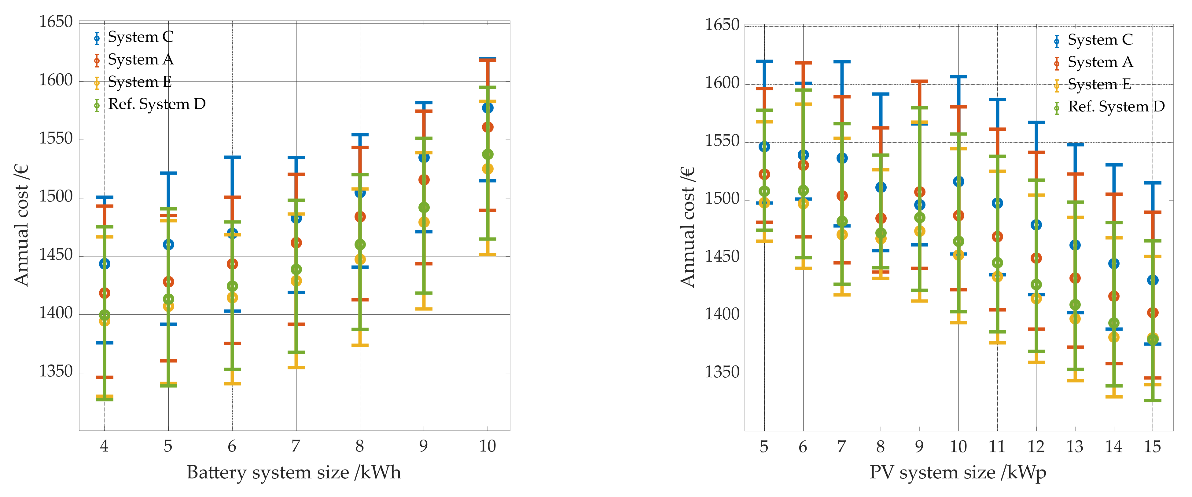
The total electricity costs are between 1327 € and 1620 € per year, depending on the PV system battery combination (see Figure 15). If the electricity demand is covered only from the grid without a PV storage system, the average annual electricity costs are 1479 €/year.

Since the dependency between costs and system combination is the same, regardless of whether the costs are presented in €/kWh or in € per year, the costs for the following parameters are only presented in €/kWh. A change in electricity costs of 1 cent/kWh leads to a change in electricity costs of 42.13 €/y and 842.64 € within 20 years.

Figure 16. Change in electricity costs per kWh of the reference case to the 3 other simulations with the battery inverter efficiency curve of system C, A and E as a function of the battery system size (left panel). Electricity costs per kWh as a function of the PV system size (right panel). Simulations were performed with the efficiency curves of systems A and D with an average pathway efficiency of 95.51 and 96.29% for the path PV2AC.

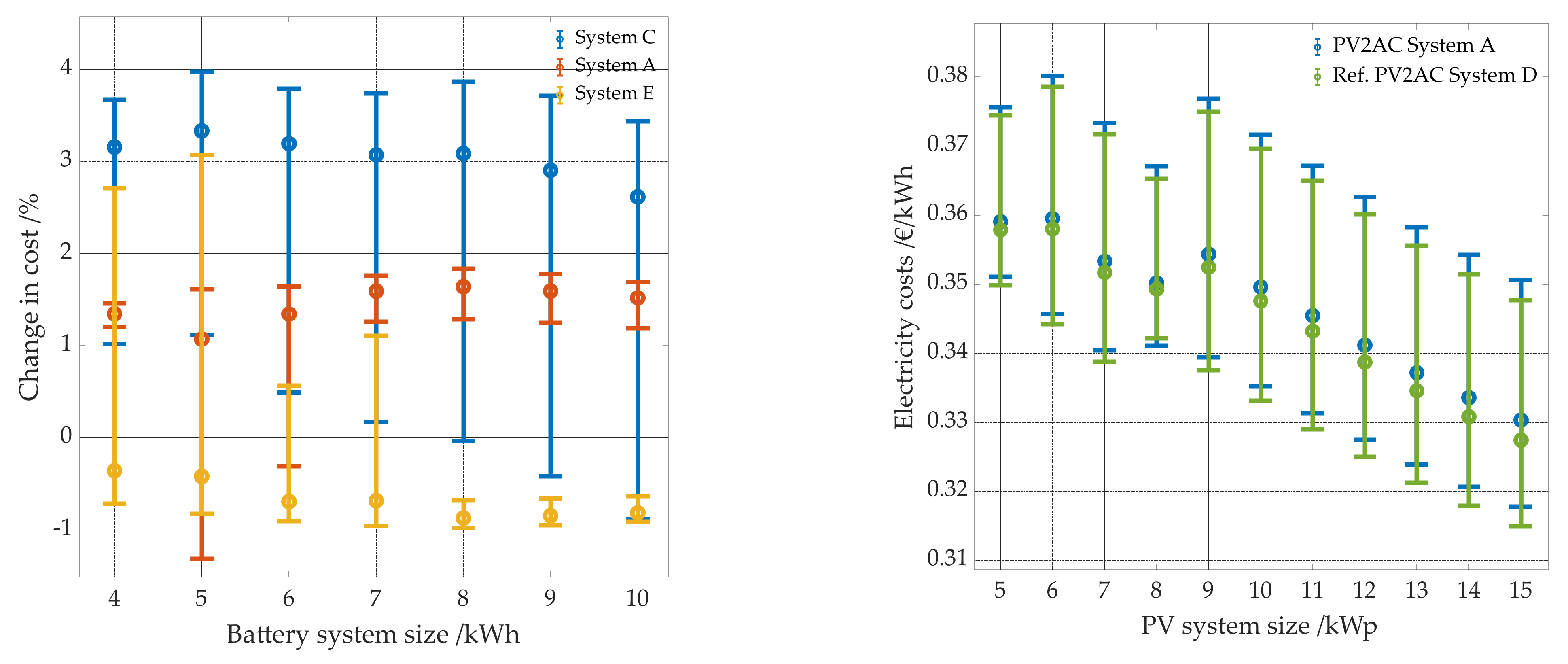
Figure 16. Change in electricity costs per kWh of the reference case to the 3 other simulations with the battery inverter efficiency curve of system C, A and E as a function of the battery system size (left panel). Electricity costs per kWh as a function of the PV system size (right panel). Simulations were performed with the efficiency curves of systems A and D with an average pathway efficiency of 95.51 and 96.29% for the path PV2AC.

The influence of the PV inverter efficiency on electricity cost represents a fairly linear relationship between cost and PV system size (see Figure 16 right panel) and battery size. The larger the PV system, the greater the advantage of a more efficient PV inverter. However, it must be taken into account that with a declining feed-in tariff, the effect for larger PV systems will decrease.

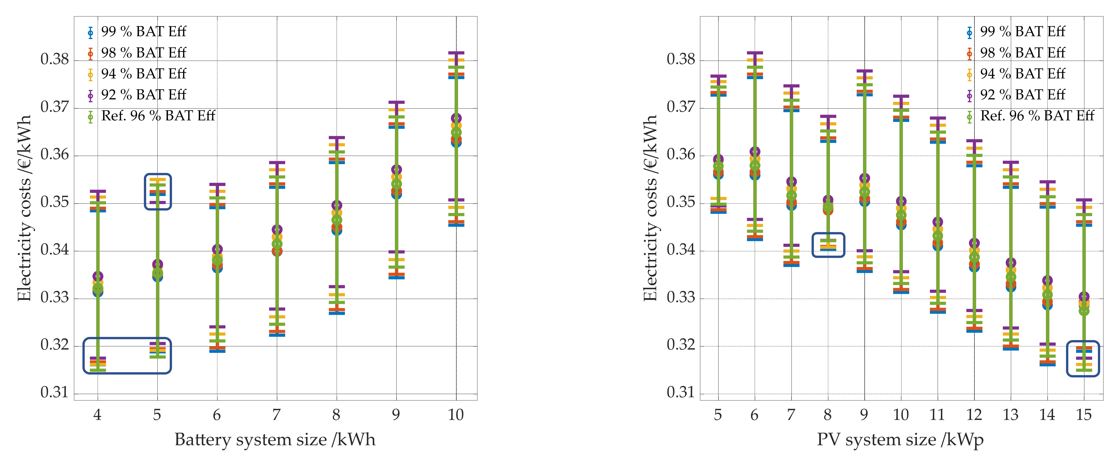
4.2.2. Effects of the Efficiency of the Battery

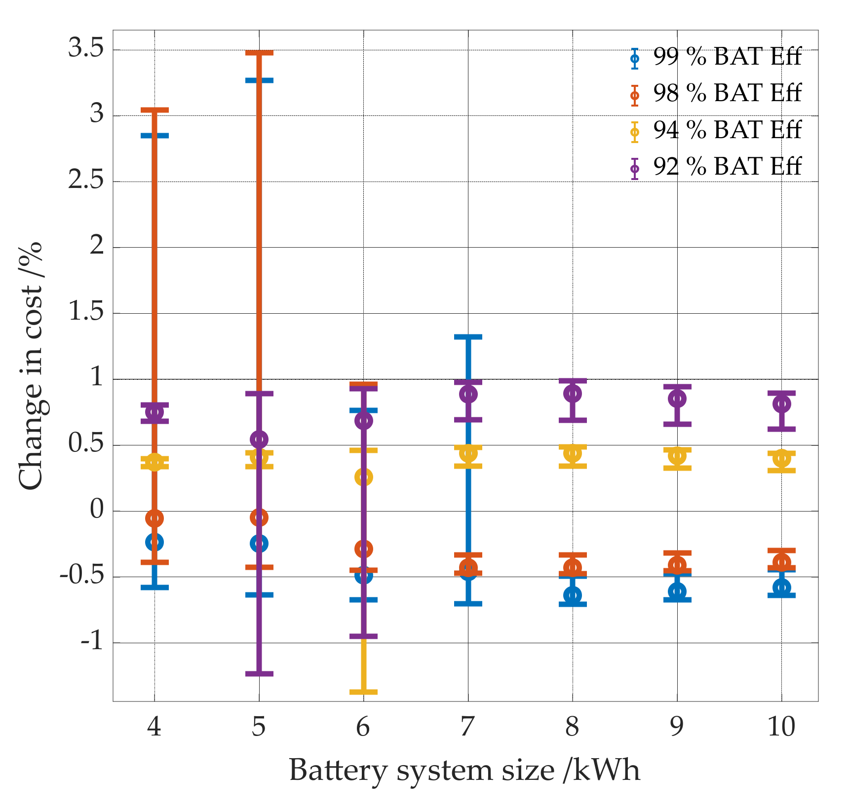
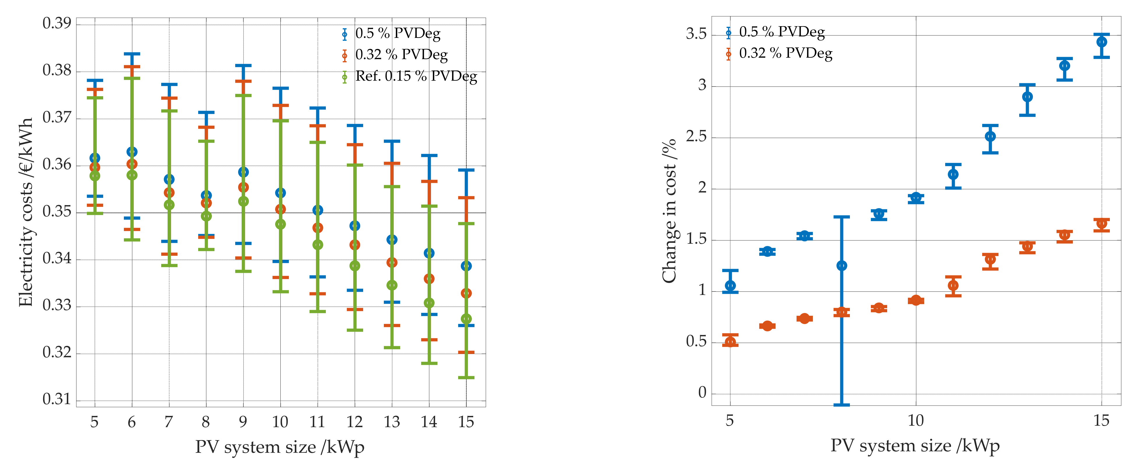
Battery efficiency has similar effects as power electronics efficiency on electricity costs. While electricity costs for large batteries decrease with increasing battery efficiency, they increase in some cases for smaller batteries of 4 kWh and 5 kWh storage capacity (see Figure 17 left panel and Figure 18). For both 4 kWh and 5 kWh, the electricity costs of the reference case are lower than those of the systems with the more efficient batteries with 98 and 99% battery efficiency. A direct comparison of the costs of these combinations shows that they increase significantly with higher battery efficiency (see Figure 18). Again, this is due to greater calendar aging as they spend a longer period of time at high SOC states. From a battery size of 6 kWh and 7 kWh, the effect decreases significantly and no longer occurs with the assumed boundary conditions in this paper from a battery size of 8 kWh. The effect occurs here as well for PV system battery combinations with a PV system size of 15 kWp and a battery capacity of 4 kWh and 5 kWh as well as with a PV system of 8 kWp and a battery capacity of 6 kWh and 7 kWh. (see Figure 17 right panel). The overall change in electricity costs between all combinations of the different variations range between −1.4% and 3.8% compared to the reference case.

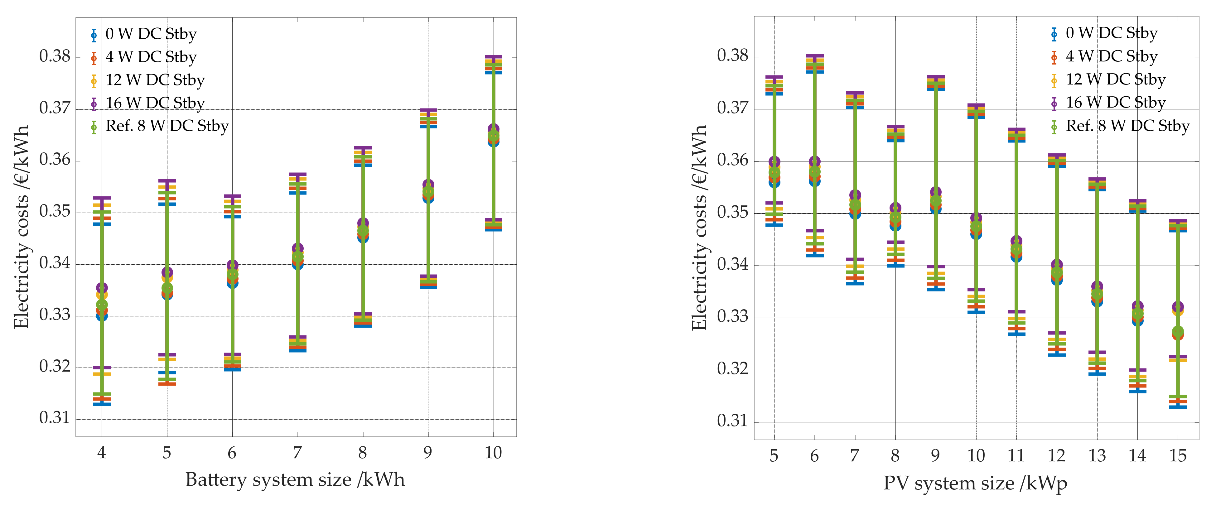
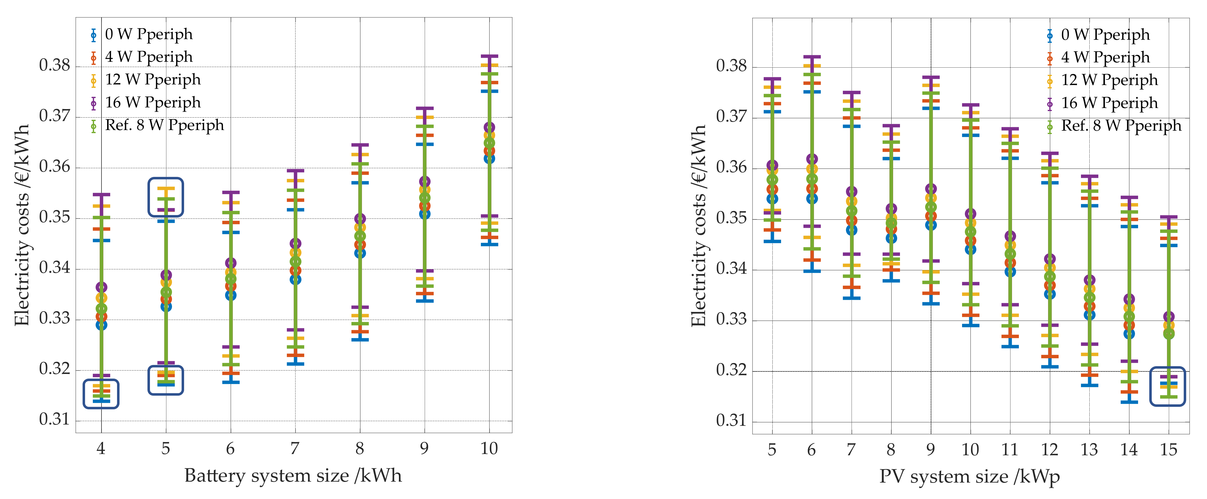
4.2.3. Effects of Standby Consumption

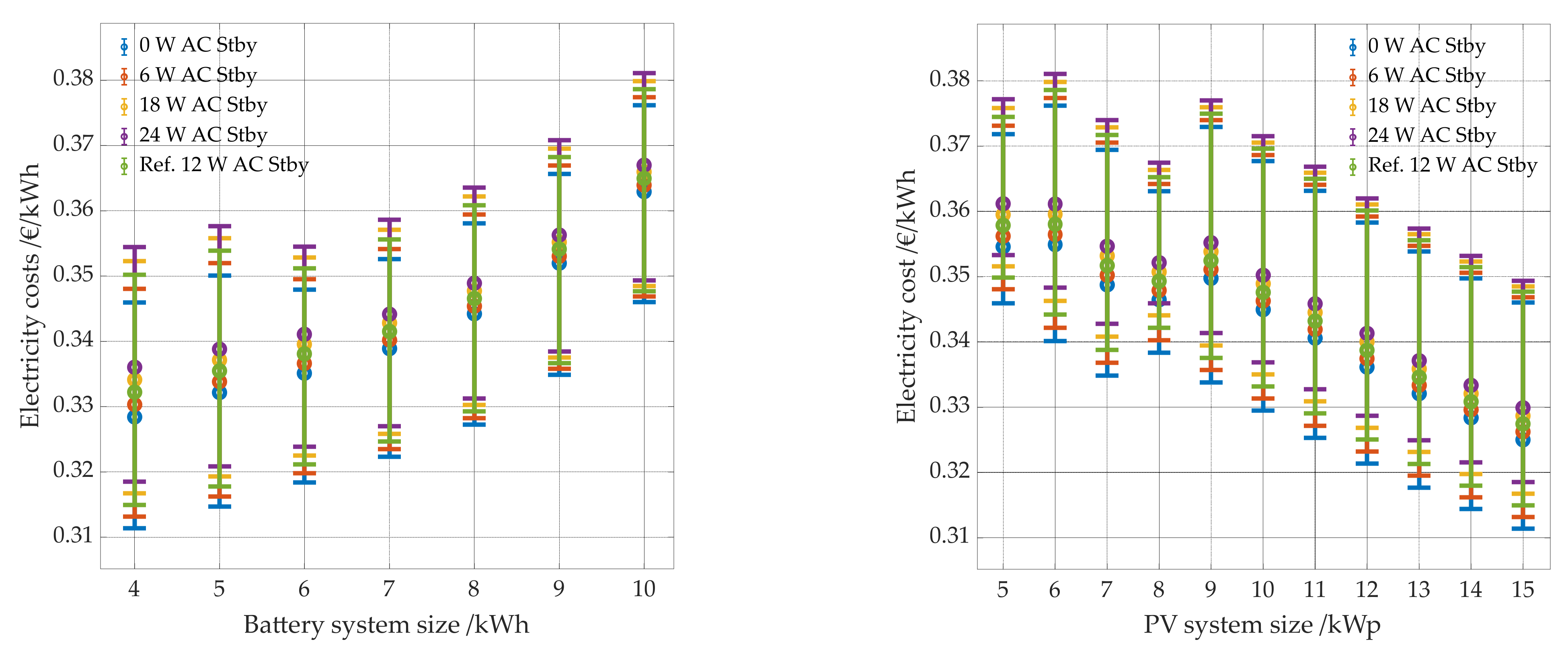
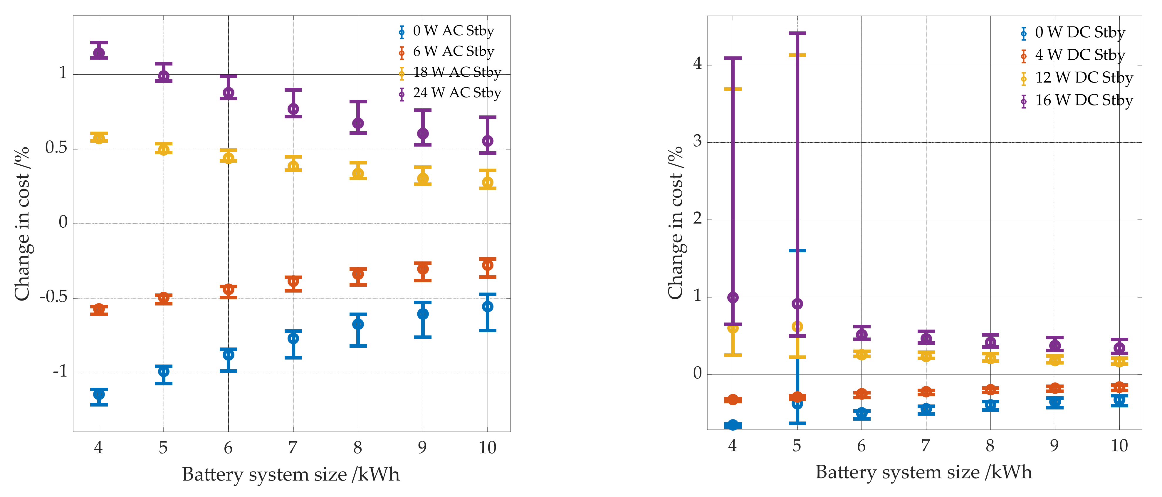
In this section the influence of the AC and DC standby as well as the peripheral consumption is examined. In contrast to the efficiencies, the lower the AC standby consumption, the lower the electricity costs for all combinations (see Figure 19). The smaller the battery or PV system, the greater the cost reduction. However, the effect is more significant for the battery. Figure 20 (left panel) shows the correlation between the change in costs for each PV system battery combination and the battery size. The cost change between a system with 0 W standby consumption and one with 24 W is up to 2.3% for the smaller batteries. The reason for this is that AC standby consumption always occurs when the battery is full or empty. Smaller batteries spend much more time in a completely empty or full state, as they become full or empty more quickly. Thus, the change in the level of standby consumption has a greater impact on the electricity cost of smaller batteries than on the electricity cost of larger ones.

The effect of DC standby consumption is quite similar to that of AC standby consumption, as DC standby consumption only occurs when the battery is full or empty as well (see Figure 21). However, the costs for combinations of batteries with 4 kWh and 5 kWh and a PV system of 15 kWp and a DC standby consumption of 12 W and 16 W are 3.7 to 4.5% higher than the costs of these combinations of the reference case. Since the batteries continue to be slightly discharged and then recharged in both the empty and fully charged states, cyclic aging increases so much for the mentioned combinations (with batteries of 4 kWh and 5 kWh and a large PV system) that they need to be replaced a year earlier than those of the reference case. The combination of a smaller battery and larger PV system results in the batteries being fully charged faster and thus being in this condition for a longer time. For all other PV system battery combinations and a DC standby consumption of 12 W and 16 W, the costs only increase by 0.6%.

Figure 21. Electricity costs per kWh as a function of battery system size (left panel) and PV system size (right panel). The results for different levels of DC standby consumption are shown in color. The reference case with an DC standby consumption of 8 W is shown in green.

Figure 21. Electricity costs per kWh as a function of battery system size (left panel) and PV system size (right panel). The results for different levels of DC standby consumption are shown in color. The reference case with an DC standby consumption of 8 W is shown in green.

Figure 22. Electricity costs per kWh as a function of battery system size (left panel) and PV system size (right panel). The results for different levels of peripheral consumption are shown in color. The reference case with a peripheral consumption of 8 W is shown in green.

Figure 22. Electricity costs per kWh as a function of battery system size (left panel) and PV system size (right panel). The results for different levels of peripheral consumption are shown in color. The reference case with a peripheral consumption of 8 W is shown in green.

In addition, it is interesting to note that with a 5 kWh battery and 4 W and 8 W DC standby consumption, the electricity costs of the cheapest combination are lower than with a 5 kWh battery and 0 W DC standby consumption. In this case, the calendar aging increases compared to the case with 4 W and 12 W DC standby consumption, because the battery is in a fully charged state for a longer period of time. The larger the PV system and the battery, the less the DC standby consumption matters.

Through the variation of the peripheral consumption in the simulation, similar effects can be observed as with the other standby consumptions (see Figure 22). Lower standby consumption can lead to the smaller batteries being fully charged sooner in combination with a large PV system, leading to increased calendar aging and the need to replace the batteries sooner.

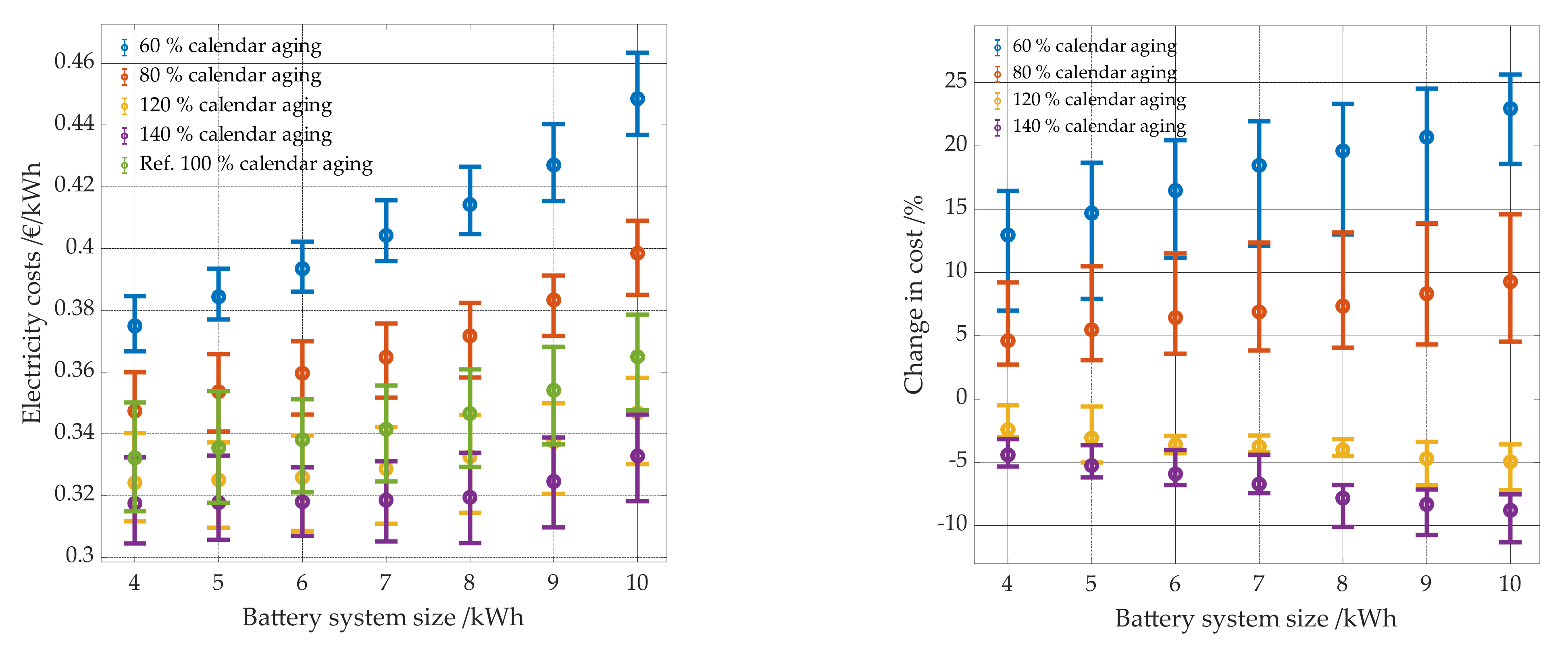
4.2.4. Effects of Battery Aging and PV Degradation

Both calendar and cyclic aging have a significant impact on the economics of PV battery storage systems.

Figure 23. Electricity costs per kWh as a function of battery system size (left panel) and the change in cost as a function of battery size (right panel). The results for different degrees of calendrical aging are shown in color. The reference case is shown in green.

Figure 23. Electricity costs per kWh as a function of battery system size (left panel) and the change in cost as a function of battery size (right panel). The results for different degrees of calendrical aging are shown in color. The reference case is shown in green.

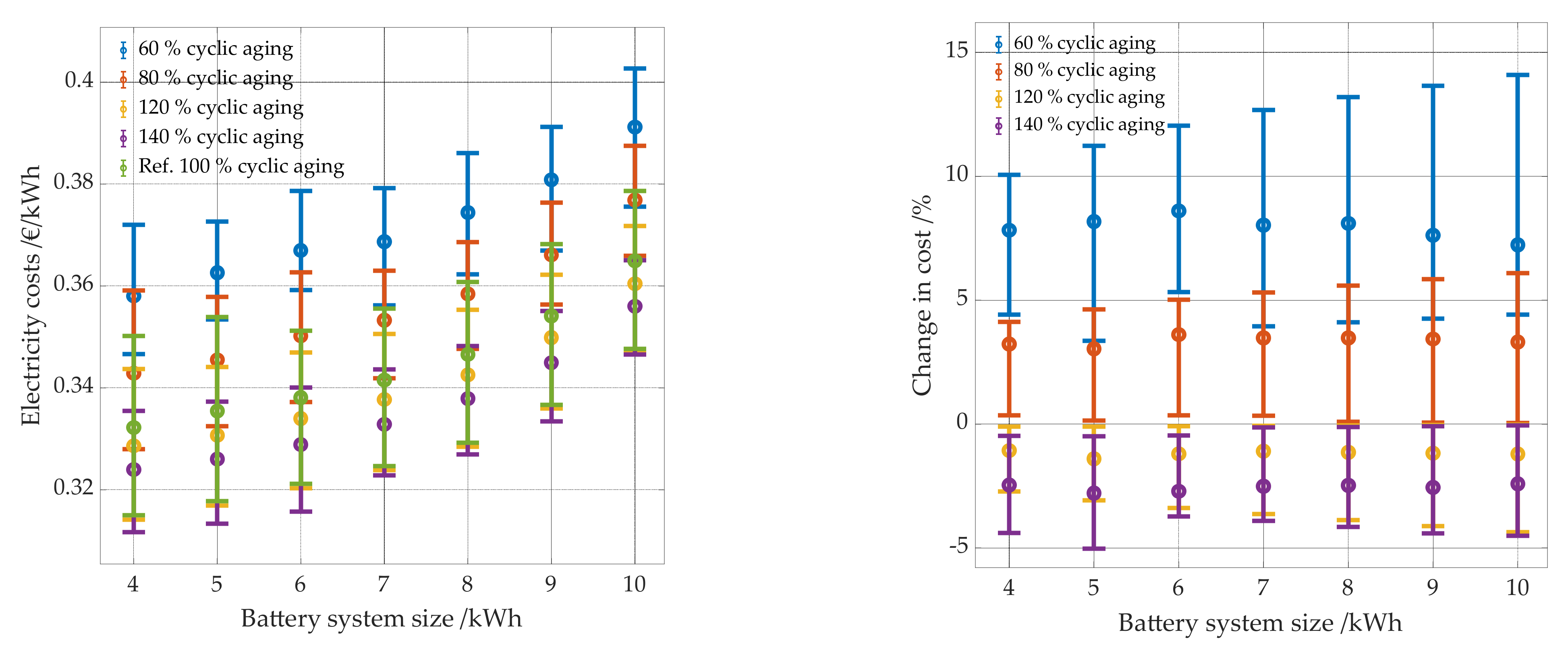
Figure 24. Electricity costs per kWh as a function of battery system size (left panel) and the change in cost as a function of battery size (right panel). The results for different degrees of cyclic aging are shown in color. The reference case is shown in green.

Figure 24. Electricity costs per kWh as a function of battery system size (left panel) and the change in cost as a function of battery size (right panel). The results for different degrees of cyclic aging are shown in color. The reference case is shown in green.

In the case of calendar aging, variations are examined in which the battery either has a 20% or 40% higher (80% calendar aging or 60% calendar aging compared to the reference case) or lower (120% calendar aging or 140% calendar aging compared to the reference case) susceptibility to calendar aging (see Table 4 and Section 3.2.2). Figure 23 shows the energy costs as a function of the battery size and the specified aging. A 20 or 40% higher susceptibility to calendar aging than that of the reference case has a significantly greater effect on the energy costs than a 20 or 40% lower susceptibility. In the case of the variations in which the susceptibility is 40% higher, the battery must be replaced already after 6 years for some PV system battery combinations. This applies to most combinations with a PV system larger than 8 kWp to 9 kWp. Since the electricity costs increase the larger the battery, the electricity costs increase significantly the higher the aging of the battery. However, this effect decreases as susceptibility to calendar aging decreases. Calendar aging of high-quality batteries used in home storage systems is currently similar to that of the reference case. However, it can be seen that the batteries should not be more susceptible to calendar aging, as this significantly affects the profitability. A lower susceptibility to calendar aging would still bring advantages, but the lower the susceptibility to calendar aging, the lower the advantage.

There is no direct functional relationship between calendar aging of the battery and the PV system size. However, with an increased susceptibility to calendar aging of 40% (60% calendar aging), the electricity costs for system combinations with a PV system between 5 kWp and 8 kWp increase at least between 7 and 21%, with a PV system size of 9 kWp and larger it is between 10 and 26%. This, however, can only be observed for the simulation with a 40% higher susceptibility to calendar aging. The larger the PV system, the more often the battery is fully charged, which leads to increased aging. With a battery that ages 40% less in terms of calendar aging, electricity costs drop by up to 11%.

Similar effects to those of calendar aging can be observed regarding the influence of cyclic aging on economic efficiency and system sizing (see Figure 24). However, a more cycle-stable battery mostly results in lower cost savings than a battery which is more susceptibility to calendar aging.

In the case of a more cycle-stable battery, electricity costs drop by up to 5%. However, it applies equally to all battery sizes. As with calendar aging, less cost savings can be achieved by a more cycle-stable battery than costs increase regarding a more cycle-unstable battery. For the reference case and the simulations with a 20 and 40% more cycle-stable battery (120 and 140% cyclic aging), the combinations with the lowest achievable electricity costs are very close to each other. Combinations with a PV system greater than or equal to 12 kWp lead to an increased cost increase for the more cycle-instable variations (60% cyclic aging, 80% cyclic aging). Due to the larger PV systems, the batteries are stressed more and therefore age faster.

The larger the PV system, the greater the cost reduction due to lower PV degradation (see Figure 25 left panel).

Figure 25. Electricity costs as a function of the PV System size (left panel) and the change in cost as a function of PV system size (right panel). Shown in color are different levels of degradation of the PV system.

Figure 25. Electricity costs as a function of the PV System size (left panel) and the change in cost as a function of PV system size (right panel). Shown in color are different levels of degradation of the PV system.

The often-assumed value of 0.5% degradation per year leads to approx. 3.5% higher costs for a 15 kWp PV system in combination with a battery than with the assumed degradation of 0.15% per year. Interesting effects occur for the combination of an 8 kWp PV system and a 6 kWh battery (see Figure 25 right panel). The cost increase of this combination is much lower than for all other simulated combinations due to the increase from 0.15 to 0.5% degradation. While at 0.15% degradation the battery has to be replaced twice in the 20 years, at 0.5% degradation it has to be replaced only once. Due to the higher amount of PV energy generated, the battery is more stressed at 0.15% degradation, ages faster and needs to be replaced earlier.

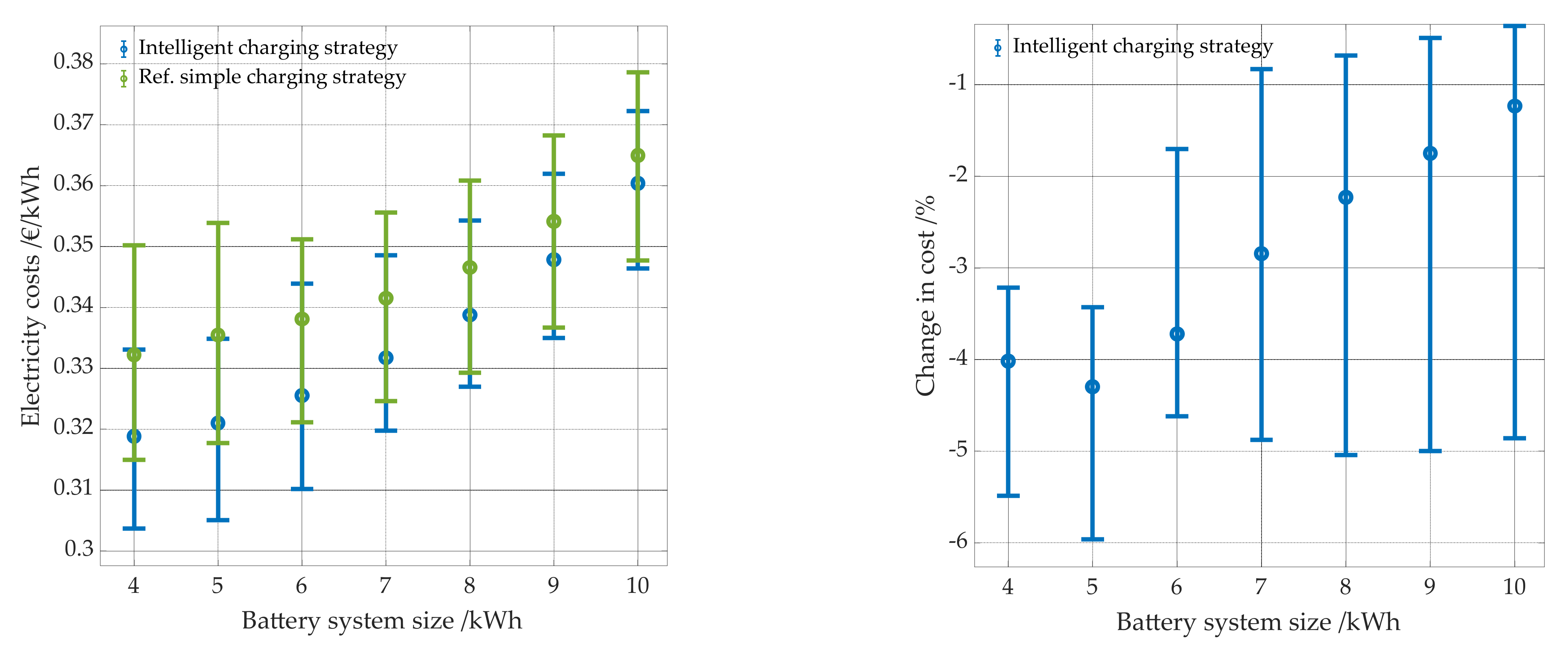
4.2.5. Effects of an Intelligent Charging Strategy

With an intelligent charging strategy, the resulting electricity costs decrease significantly. The smaller the battery, the greater the cost savings (see Figure 26). The largest reduction with 6% can be achieved with 8 kWp and a 5 kWh battery. The intelligent charging strategy is primarily used to reduce the time the battery spends in high SOC states. Without an intelligent charging strategy, a 4 kWh battery in combination with a PV system of 15 kWp spends 35.07% of its time at a SOC greater than 80% and only 17.07% with an intelligent charging strategy. Without an intelligent charging strategy, the battery has to be replaced after 9 and after 18 years, with an intelligent charging strategy only after 10 years and thus only once instead of twice within the 20 years.

Under Section 4.1.2, the impact of an electricity price increase is discussed. It is shown that system combinations of a PV system smaller than 11 kWp and a battery with at least 4 kWh storage capacity are no longer economical. However, by using an intelligent charging strategy, the costs can be reduced to such an extent that combinations with PV systems between 5 kWp and 10 kWp are economically viable against grid consumption, depending on the installed battery size. However, the same does not apply for any combination with a battery with 7 kWh and more.

Figure 26. Electricity costs per kWh as a function of battery system size (left panel) and the change in cost as a function of battery size (right panel). Shown are the results for a and an intelligent charging strategy to prevent calendar aging. The reference case is shown in green.

Figure 26. Electricity costs per kWh as a function of battery system size (left panel) and the change in cost as a function of battery size (right panel). Shown are the results for a and an intelligent charging strategy to prevent calendar aging. The reference case is shown in green.

5. Discussion

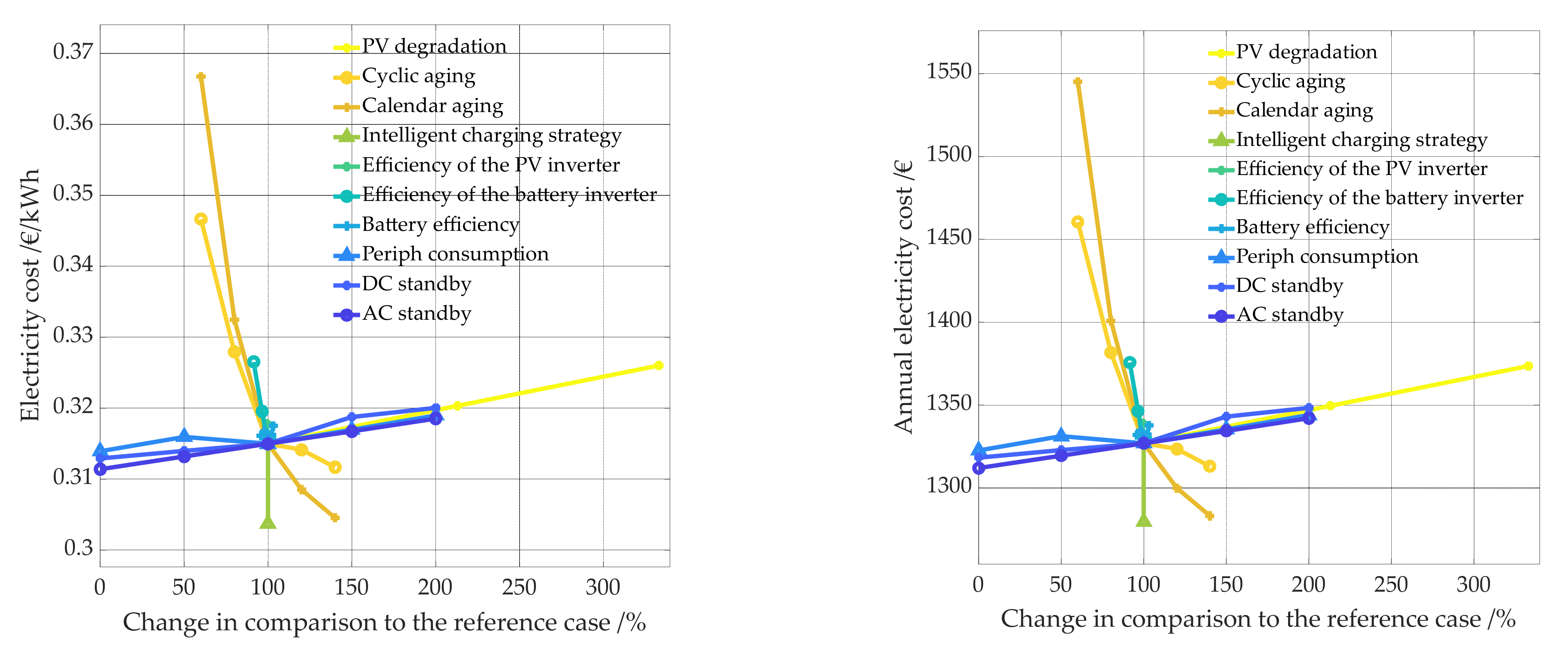
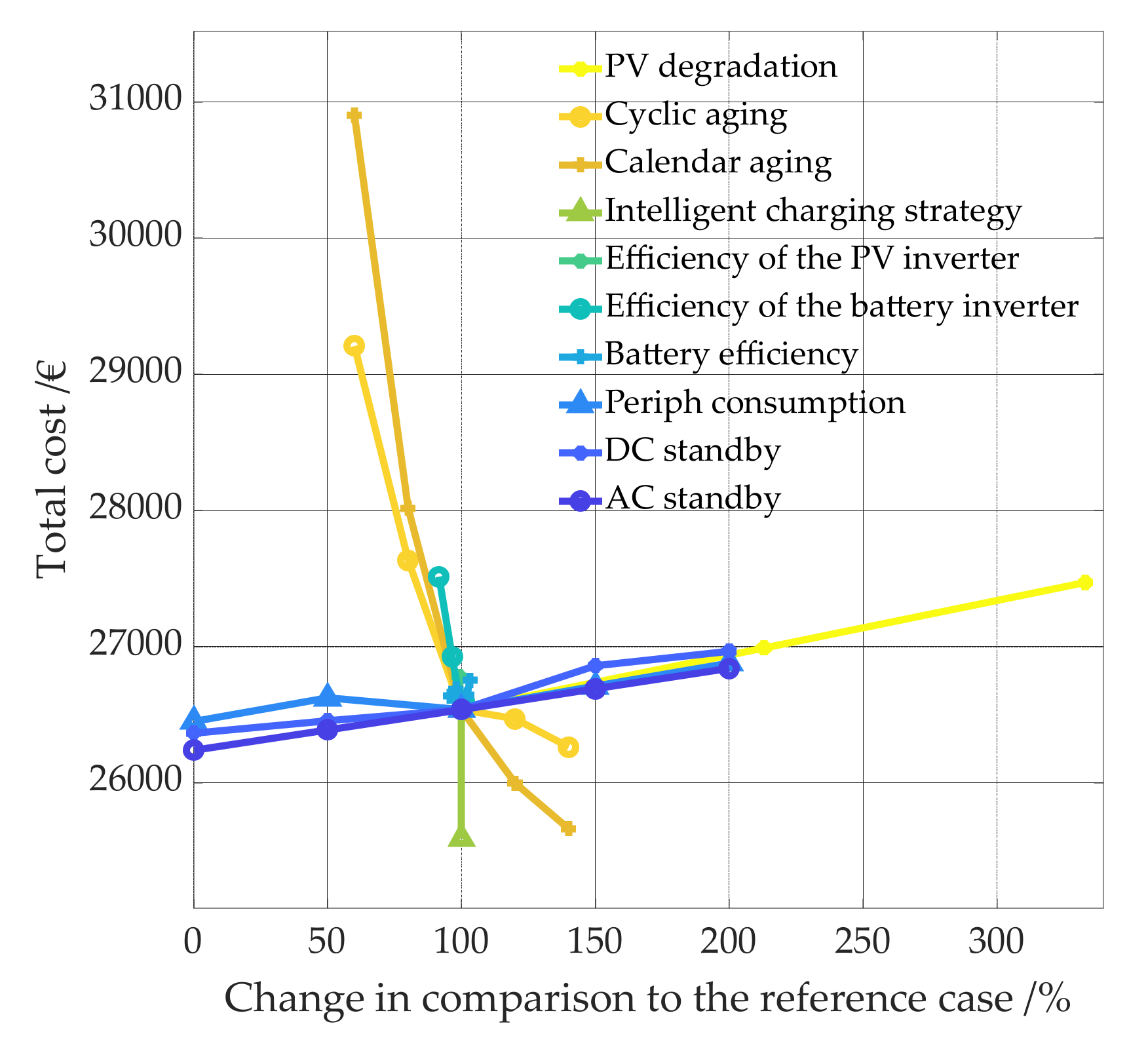
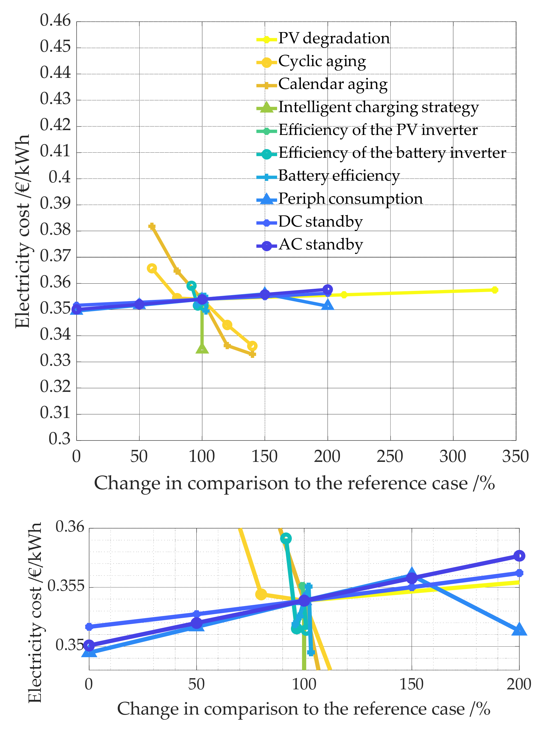
In the following, the impact on electricity costs due to the change in technical parameters is presented and compared to each other. For this purpose, 6 PV system battery combinations are examined in more detail. On the one hand, the most favorable combination for each simulation run carried out (see Figure 27 and Figure 28) is examined. On the other hand, the PV system battery combinations 15 kWp PV system with 10 kWh battery and 5 kWh battery (see Figure 29), 10 kWp PV system with 10 kWh and 5 kWh battery (see Figure 30) and 5 kWp PV system with 5 kWh battery (see Figure 31) are examined. Figure 27 and Figure 28 show the electricity costs for the most favorable combination for each simulation run. The left panel of Figure 27 shows the electricity costs per kWh and the right panel the annual costs.

Figure 28 shows the total electricity costs for the 20 years under consideration. As mentioned a change in electricity costs of 1 cent/kWh leads to a change in electricity costs of 42.13 €/y and 842.64 € within 20 years. A detailed overview over the cost in cent/kwh, €/y and over 20 years in shown in

Table A3. Electricity costs in €/kWh depending on the change of different technical parameters. The selected PV system and battery combination is the combination that is the most favorable for the respective boundary conditions.

	AC Stby	DC Stby	Pperiph	η Battery	η Battery Inverter	η PV Inverter	Charging Strategy	Calendar Aging	Cyclic Aging	PV Degradation
V1	31.14	31.29	31.39	31.61	32.65	31.78	30.37	36.67	34.67	32.60
V2	31.32	31.40	31.59	31.67	31.95	31.50	31.50	33.25	32.79	32.03
Ref.	31.50	31.50	31.50	31.50	31.50			31.50	31.50	31.50
V3	31.67	31.88	31.70	31.62	31.57			30.85	31.41
V4	31.85	32.00	31.90	31.75				30.46	31.17

,

Table A4. Electricity costs per year in € depending on the change of different technical parameters. The selected PV system and battery combination is the combination that is the most favorable for the respective boundary conditions.

	AC Stby	DC Stby	Pperiph	η Battery	η Battery Inverter	η PV Inverter	Charging Strategy	Calendar Aging	Cyclic Aging	PV Degradation
V1	1312	1318	1323	1332	1376	1339	1280	1545	1461	1374
V2	1319	1323	1331	1334	1346	1327	1327	1401	1382	1350
Ref.	1327	1327	1327	1327	1327			1327	1327	1327
V3	1334	1343	1335	1332	1330			1300	1323
V4	1342	1348	1344	1338				1283	1313

and

Table A5. Total electricity costs over a period of 20 year in € depending on the change of different technical parameters. The selected PV system and battery combination is the combination that is the most favorable for the respective boundary conditions.

	AC Stby	DC Stby	Pperiph	η Battery	η Battery Inverter	η PV Inverter	Charging Strategy	Calendar Aging	Cyclic Aging	PV Degradation
V1	26,240	26,367	26,453	26,638	27,514	26,782	25,592	30,902	29,210	27,471
V2	26,390	26,457	26,623	26,689	26,927	26,540	26,540	28,015	27,634	26,992
Ref.	26,540	26,540	26,540	26,540	26,540			26,540	26,540	26,540
V3	26,690	26,861	26,709	26,646	26,601			25,998	26,470
V4	26,840	26,967	26,879	26,753				25,663	26,262

in the Appendix A.

The most favorable PV system size for each simulation run can be seen in

Table 6. PV system size of the most economic combination of the different simulation runs with the different technical parameter.

	AC Stby	DC Stby	Pperiph	η Battery	η Battery Inverter	η PV Inverter	Charging Strategy	Calendar Aging	Cyclic Aging	PV Degradation
V1	15	15	14	14	15	15	15	15	15	15
V2	15	15	14	14	15			14	15	15
Ref.	15	15	15	15	15	15	15	15	15	15
V3	15	14	15	15	14			15	15
V4	15	14	15	15				15	13

. In most cases it consists of a 15 kWp PV system, which is the largest PV system size analyzed. Thus, it could be that the most economical PV system size is even higher. In many cases, however, the roof area is limited, which is why the investigations were only carried out up to a system size of 15 kWp. In some cases, the optimal size drops to 13 kWp and 14 kWp. This is the case, for example, with decreasing DC standby consumption, increasing battery inverter efficiency, decreasing battery efficiency, increasing peripheral consumption and higher cycle stability. The optimal battery size in almost all cases is 4 kWh, which is the smallest battery size analyzed. For the 20 less susceptibility to calendar aging, the optimal battery size increases to 6 kWh, respectively.

With decreasing standby consumption compared to the reference case, decreasing AC standby consumption has a greater positive impact on electricity costs than decreasing DC standby consumption and decreasing peripheral consumption. With increasing standby consumption compared to the reference case, increasing DC standby consumption has the most negative impact on electricity costs. The percentage increase in PV degradation per year has a similar impact on electricity costs as increasing standby consumption. Faster aging batteries, both in terms of calendar and cyclic aging, and declining battery inverter efficiency have a very high impact on electricity costs. Their impact is significantly higher than that of standby consumption. In contrast, it is interesting to note that when the battery inverter efficiency is higher than the reference case, the electricity cost increases again slightly. This is as explained under Section 4.2.1 due to increased battery aging and earlier battery replacement, as the battery is charged more with the more efficient inverter. While, as explained, batteries with less cycle stability than the one of the reference case result in a very large cost increase, a further increase in cycle stability results in only a small cost reduction. Also, batteries that have a higher susceptibility to calendar aging than the batteries of the reference case, the cost reduction is less than the costs increase by batteries that have a higher susceptibility to calendar aging. However, this change is less significant than in the case of cyclic aging. A very high cost reduction is achieved by using an intelligent charging strategy. For the most favorable combination for each simulation run carried out a change in battery efficiency always leads to higher costs. The cost increase is as high as the increase due to the less efficient PV inverter and as high as a 50% increase in standby consumption.

Figure 29, Figure 30 and Figure 31 show how the change in technical parameters affects other PV system battery combinations. Most of the changes affect all PV system battery combinations in a similar way. However, some changes have much higher or lower impacts. For the following comparisons, only the costs in €/kWh are shown, since only the y-axis scaling changes for the costs per year and the costs in 20 years. Remember, a cost increase of 1 cent/kWh leads to a cost increase of 42.13 €/y and 842.64 € in 20 years.

A less efficient battery inverter in contrast to that of the reference case leads to significantly higher electricity costs in almost all cases. These are between 0.53 cent/kWh and 1.3 cent/kWh and 22.16 €/y and 54.76 €/y higher than those of the reference case. For the combinations with a PV system with 10 kWp or15 kWp and a 10 kWh or 5 kWh battery, they are higher than for the other combinations investigated.

For the combinations 15 kWp/10 kWh, 10kWp/10 kWh and 10 kWp/5 kWh the influence of the change of AC standby, DC standby and peripheral consumption is very close to each other and follows a slightly increasing linear function for both an increase of the standby consumption and a reduction. The increase is flatter the larger the battery and the larger the PV system relative to the household load. The reason for this is that a slight increase or decrease in energy charged to or discharged from the battery is less significant for a relatively large battery than for a relatively small one. In contrast, for a 15 kWp PV system with a 5 kWh battery, both the increase to 12 W and 16 W and a reduction to 0 W DC standby consumption result in significantly higher costs.

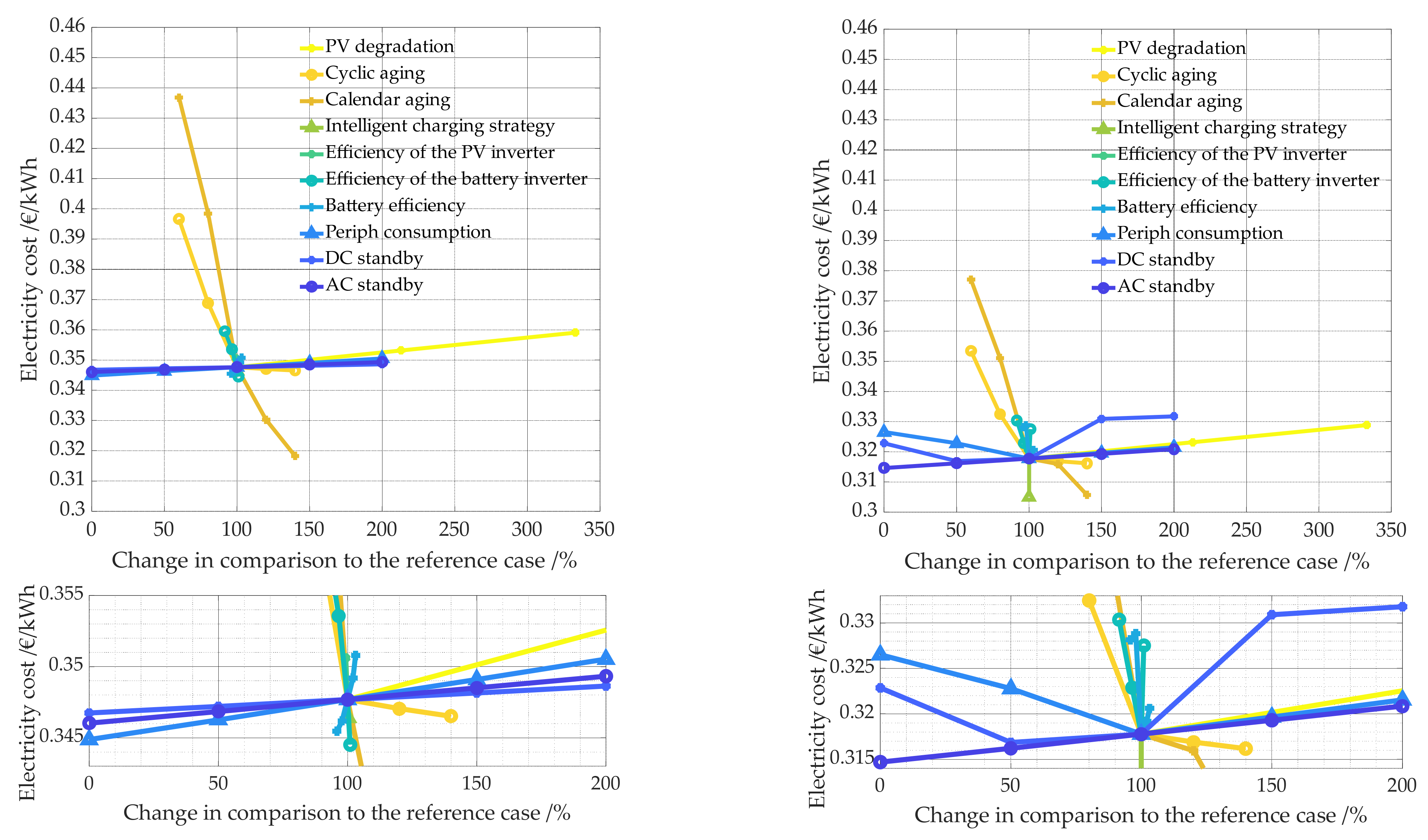
Figure 29. Impact on electricity costs due to the change in technical parameters. The left panel shows the PV system battery combination of 15 kWp and 10 kWh, the right one of 15 kWp and 5 kWh. While the upper figures show all data points, the lower figures show only parts of the data in order to better illustrate even small changes in relation to the reference case.

Figure 29. Impact on electricity costs due to the change in technical parameters. The left panel shows the PV system battery combination of 15 kWp and 10 kWh, the right one of 15 kWp and 5 kWh. While the upper figures show all data points, the lower figures show only parts of the data in order to better illustrate even small changes in relation to the reference case.

Figure 30. Impact on electricity costs due to the change in technical parameters. The left panel shows the PV system battery combination of 10 kWp and 10 kWh, the right one of 10 kWp and 5 kWh. While the upper figures show all data points, the lower figures show only parts of the data in order to better illustrate even small changes in relation to the reference case.

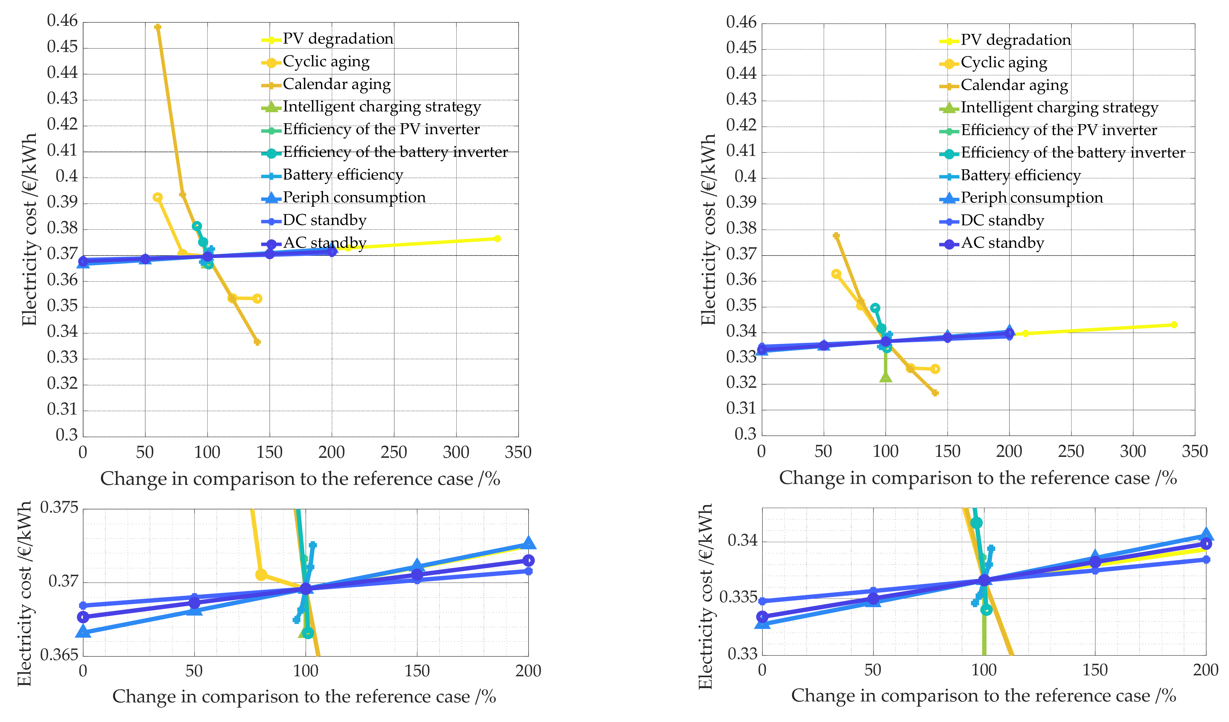
Figure 30. Impact on electricity costs due to the change in technical parameters. The left panel shows the PV system battery combination of 10 kWp and 10 kWh, the right one of 10 kWp and 5 kWh. While the upper figures show all data points, the lower figures show only parts of the data in order to better illustrate even small changes in relation to the reference case.

Figure 31. PV system battery combination of 5 kWp and 5 kWh. While the upper figures show all data points, the lower figures show only parts of the data in order to better illustrate even small changes in relation to the reference case.

Figure 31. PV system battery combination of 5 kWp and 5 kWh. While the upper figures show all data points, the lower figures show only parts of the data in order to better illustrate even small changes in relation to the reference case.

In both cases, this is due to a greater stress on the battery. While in the case of the reduction of the DC standby consumption calendar aging increases, in the case of the increase of DC standby consumption cyclic aging increases. The same applies to the reduction of the peripheral consumption to 0 W with a 15 kWp PV system and a 5 kWh battery; here, too, the increased charging of the battery leads to increased aging of the battery and earlier replacement. The opposite is the case for the PV system battery combination with a 5 kWp PV system and a 5 kWh battery and an increase of the peripheral consumption by 100% to 16 W.

The cost-reducing effect of a battery that is more resistant to calendar aging is higher than the cost-reducing effect of a more cycle-stable battery for all combinations investigated. Especially with a battery that is more susceptible to calendar aging, the costs increase strongly. If the battery is actually 40% more susceptible to calendar aging than the reference case, the costs can increase by 2.79 cent/kWh to 8.91 cent/kWh, depending on the combination. This would result in a cost increase of 117.73 €/y and 375.48 €/y. As already mentioned in Section 4.2.4, however, the costs decrease less if the battery is less susceptible to calendar aging than the reference case.

An intelligent charging strategy has a large positive effect on electricity costs for the PV system battery combinations 5 kWp/5 kWh, 10 kWp/5 kWh and 15 kWp/5 kWh. For a 5 kWp PV system with a 5 kWh battery, the positive impact is almost the same as from a battery that would have a 40% less susceptibility to calendar aging. Depending on the combination, electricity costs can be reduced by between 1.27 cent/kWh and 1.92 cent/kWh (53.54 €/y and 80.71 €/y). However, the positive effect decreases the larger the PV system is. For the combination 10 kWp/10 kWh the positive effect decreases significantly. For 15 kWp/10 kWh, almost no positive effect can be observed anymore.

The larger the PV system and the battery are, the higher the influence of the degradation of the PV system on the electricity costs. The often assumed 0.5% degradation of the PV system leads to 1.14 cent/kWh or 48.10 €/y higher electricity costs for the PV system battery combination of 15 kWp and 10 kWh than for the reference case.

The average cost of electricity purchased from the grid is 35.11 cent/kWh, resulting in 1479 €/y. Apart from the combinations of 10 kWp PV and 10 kWh battery and a 5 kWp PV and a 5 kWh battery, the reference case would be more favorable for all other combinations examined in more detail. The combination of a 10 kWp PV system and a 10 kWh battery would only be more economic than purchasing electricity from the grid if the batteries were less susceptibility to calendar aging (see Figure 30 left panel). The combination of a 5 kWp PV system and a 5 kWh battery would be more economic if the batteries were less susceptible to calendar aging or more cycle stable, with 0 W AC standby consumption or peripheral consumption, a more efficient battery, an intelligent charging strategy.

PV inverters are usually already very efficient. With the slightly worse inverter (0.78 percentage points less in in the average pathway efficiency), the electricity cost of all variations increased slightly. The larger the PV system, the greater the cost increase. At most, the less inefficient PV inverter increases the cost by only 0.29 cent/kWh, which is 12.37 €/year.

Both higher and lower battery efficiency can result in higher as well as slightly lower costs. The highest cost increase occurs for the PV-system battery combination of 15 kWp PV and a 5 kWh battery (see Figure 29 right panel). It is 1.1 cent/kWh or 46.55 €/y, which is significantly higher than the electricity cost increases caused by standby consumption, for example for this PV system, battery combination. For all other combinations, the electricity cost increase is at most 0.31 cent/kwh and 13.10 €/y and is thus in the range of standby consumption or below. This has already been explained in more detail in Section 4.2.2.

For almost all technical parameters examined here, a change for the worse compared to the reference case has a significantly greater negative impact on costs than a further improvement has positive effects. An overview of the maximum changes through V1 to V4 of the individual technical parameters compared to the reference case can be found in

Table A6. Overview of the maximum changes regarding electricity cost through V1 to V4 of the individual technical parameters compared to the reference case. To calculate the total cost for the calculation period the maximum cost increase and decrease needs to be multiplied by 20.

PV System/Battery	Max Cost Increase/Decrease due to the Variations V1–V4 in Comparison to Ref.	AC Stby	DC Stby	P Periph	Eff Battery	Eff Battery Inverter	Eff PV Inverter	Charging Strategy	Calendar Aging	Cyclic Aging	PV Degradation
15 kWp/10 kWh	max cost increase cent/kWh	0.16	0.10	0.28	0.31	1.19	0.29		8.91	4.90	1.14
	max cost increase €/y	6.95	4.02	11.96	13.10	49.98	12.37		375.48	206.29	48.10
	max cost decrease cent/kWh	−0.16	−0.09	−0.28	−0.22	−0.32		−0.13	−2.94	−0.12	0.55
	max cost decrease €/y	−6.94	−3.97	−11.85	−9.35	−13.32		−5.28	−123.89	−4.86	23.32
15 kWp/5 kWh	max cost increase cent/kWh	0.31	1.40	0.87	1.10	1.26	0.29		5.93	3.57	1.11
	max cost increase €/y	12.98	59.10	36.83	46.55	53.08	12.09		249.73	150.31	46.82
	max cost decrease cent/kWh	−0.31	−0.09	0.19	0.14	0.51		−1.27	−1.20	−0.16	0.54
	max cost decrease €/y	−12.97	−3.78	7.90	5.90	21.57		−53.54	−50.56	−6.73	22.69
10 kWp/10 kWh	max cost increase cent/kWh	0.19	0.12	0.30	0.30	1.17	0.20		8.86	2.29	0.69
	max cost increase €/y	8.11	5.04	12.73	12.50	49.49	8.59		373.14	96.33	29.05
	max cost decrease cent/kWh	−0.19	−0.11	−0.30	−0.21	−0.30		−0.30	−3.30	−1.62	0.33
	max cost decrease €/y	−8.10	−4.82	−12.58	−8.93	−12.63		−12.64	−139.07	−68.22	13.89
10 kWp/5 kWh	max cost increase cent/kWh	0.32	0.18	0.39	0.28	1.30	0.20		4.11	2.63	0.65
	max cost increase €/y	13.57	7.69	16.55	11.74	54.76	8.47		172.99	110.63	27.32
	max cost decrease cent/kWh	−0.32	−0.19	−0.39	−0.20	−0.26		−1.43	−2.00	−1.07	0.31
	max cost decrease €/y	−13.56	−7.82	−16.31	−8.45	−10.96		−60.07	−84.25	−44.97	13.04
5 kWp/5 kWh	max cost increase cent/kWh	0.38	0.23	0.21	0.12	0.53	0.12		2.79	1.19	0.36
	max cost increase €/y	15.99	9.84	8.94	5.05	22.16	5.21		117.73	50.19	15.31
	max cost decrease cent/kWh	−0.38	−0.22	−0.44	−0.44	−0.25		−1.92	−2.10	−1.78	0.18
	max cost decrease €/y	−15.98	−9.37	−18.52	−18.40	−10.43		−80.71	−88.36	−74.98	7.40

in the Appendix A.

Most changes in the technical parameters have little effect on the degree of self-sufficiency. Of the combinations studied here, the change in the degree of self-sufficiency is in the range of ±0.8 percentage points. There is one exception, however. If the inverter efficiency decreases (V1 system C), the degree of self-sufficiency decreases by a maximum of 3.44 percentage points. If, on the other hand, it increases (V3 system E), the degree of self-sufficiency increases by 0.74 percentage points. The corresponding average pathway efficiencies for the battery inverters are shown in Table 2. The average pathway efficiency of inverter C is 8.8 percentage points lower for the conversion path BAT2AC and 6.33 percentage points lower for the conversion path AC2BAT. In contrast, the values for inverter E are 1.82 percentage points (BAT2AC) and 2.71 percentage points (AC2BAT) higher than those of reference system D. On average, the increase in average pathway efficiencies (mean value of the AC2BAT and BAT2AC paths) leads to an increase in the degree of self-sufficiency of 0.33 to 0.45 percentage points.

There are already studies in the literature by various authors that determine the optimal battery and or PV system size in terms of economic efficiency [10,13,22,27,30,31,40]. It is difficult to compare the results directly with each other and the findings of this paper, because in all studies different battery and PV system costs, a different feed-in tariff or grid electricity purchase price were assumed. At the same time, in some cases a higher electricity price increase is expected. In most of the studies, relatively favorable battery prices were assumed, which have not yet been achieved in the field of Li-ion home storage systems (350–600 €/kWh). In addition, Sharma et al. [23] and Ayuso et al. [40] examine only PV systems up to 4 kWp and 5 kWp respectively. While in the work of Sharma et al. [23] the most economical battery size is 5 kWh, which corresponds to the largest battery size investigated in [23], the most economical battery size determined by Ayuso et al. [40] is 3.2 kWh, which is the smallest battery size investigated in [40]. According to Weniger et al. [27] and Quoilin et al. [30], the most economical battery capacity is approx. 1 kWh per MWh energy consumption of the household per year. This is approximately in the range of the most economical battery size determined in this work. The results of Mulder et al. [10] for the year 2021 are also in a similar range. Only in Bertsch et al. [13] the most economical battery size is above 10 kWh. In addition to the very low battery costs, an electricity cost increase of 2% and an inflation rate of 2% are assumed [13]. However, all mentioned studies consider PV systems only up to a size of 10 kWp. The optimal size is in most cases between 4 kWp and 8 kWp. In contrast, the optimal PV system size determined in the present work is between 13 kWp and 15 kWp. One reason for this is the assumed costs for a PV system. In contrast to the literature, the assumed costs in the present work are dependent on the system size and decrease with increasing PV system size, per kW of installed system power. This assumption is more realistic.

As mentioned above, a detailed analysis of how the technical parameters affect the economic efficiency has not yet been carried out in literature. Only individual parameters were investigated. Tervo et al. show the sensitivity of the system levelized cost of electricity to a 10% perturbation of the PV degradation, the battery efficiency and on cyclic aging of the battery [31]. Bertsch et al. [13], Troung et al. [14] and Naumann et al. [12] also investigate the influence of cyclic aging on economic efficiency (see

Table 7. Parameters used in the literature to evaluate the influence of cycle stability on economic efficiency.

	PV System Size	Battery Size	Economical Parameter	Calendar Lifetime	Cycle Stability Variation	Battery Price
Bertsch et al. [13]	6.4 kWp	12 kWh	IRR	20 y	500 until 6000 cycles	500 €/kWh
Tervo et al. [31]	5 kWp	7 kWh	LCOE	15 y	5000 cycles ± 10%	392 $/kWh + 1700 $
Troung et al. [14]	5 kWp/8 kWp	6.4 kWh	ROI	15 y	5000 & 3000 cycles (−40%)	781.25 €/kWh
Naumann et al. [12]	4.4 kWp	4 kWh	ROI	12.5–15 y	6000 & 3000 cycles (−50%)	<500 €/kWh

). However, they use different economical parameters to compare the results. An overview of the most important parameters used in the literature can be found in Table 7.

While in Troung et al. [14] the reduction in ROI ranges from 4% to 13% with a 40% reduction in cycle stability, Naumann et al. [12] show a reduction in ROI of up to 8% with a 50% reduction in cycle stability. In contrast, the economic efficiency in the present work was not evaluated on the basis of ROI but on the basis of total electricity costs. The present work finds 3.4% to 14.1% higher electricity costs for the household due to a reduction of the cycle stability by 40%. While the increase is only 3.4% for a 5 kWp PV system combined with a 5 kWh battery, it is 10.1% for a 15 kWp PV system combined with a 4 kWh battery. Thus, the present work presents a trend similar to that found in the literature. Bertsch et al. [13] show a relatively low sensitivity of profitability to cyclic aging. In the case of Bertsch et al. [13] a relatively small PV system (6.4 kWp) is combined with a large battery (12 kWh), which leads to a relatively low cycle load of the battery. Only the reduction of the cycle stability to 2500 cycles leads to a reduction of the profitability by 2%. However, the trend shown in [13] is similar to the results in this paper, the higher the cycle stability the lower is the positive effect on the economic efficiency. Tervo et al. [31] use the aging model of [14] and conclude that a 10% change in cycle stability leads to a 0.5% change in LCOE. In the present work, the change in electricity cost due to a 10% change in cycle stability is between 0.1% and 3.0% for a less cycle stable battery and between 0.1% and 1.3% for a more cycle stable battery. It must be taken into account that in the current paper a PV system with at least as much kWp as the battery has kWh storage capacity is assumed, which leads to more cycles of the battery.

The influence of PV degradation on the economic efficiency is significantly higher in Tervo et al. [31] than in the present work, since a degradation of 0.8% per year is assumed. For [31], the influence of a 10% change in PV degradation is 0.25% to 0.5%, while in the present work it is only 0.1%.

Tervo et al. [31] assumes 90% battery efficiency and calculates an impact of approx. 2% on the LCOE with a 10% change in battery efficiency. In contrast, 96% (reference case) battery efficiency is assumed in the present work. For most PV system battery combinations, a lower battery efficiency than the reference case of 4.2% results in a cost increase of maximum 1%, which is in a similar range to the result in the literature. However as described, higher battery efficiency does not necessarily lead to lower costs, since without an intelligent charging strategy, the state of charge is higher and this in turn can have an impact on calendar aging. Thus, Figure 18 shows a maximum change in cost of up to 3.5% with an increase in battery efficiency of up to 3.1%. The difference with the literature can be explained by the fact that no SOC-dependent calendrical aging model was used in [31].

6. Conclusions and Outlook

The paper presents a new methodology for simulating and sizing PV battery storage systems that are used to increase self-consumption. The most important efficiency parameters, calendar and cyclic aging as well as the charging strategy are taken into account. The efficiency parameters considered include AC and DC standby consumption, peripheral consumption, battery efficiency and inverter efficiency of the battery and PV inverter. The developed intelligent charging strategy is primarily designed to minimize calendar aging of the battery by avoiding long periods of high SOC conditions. For the calculation of the reference case, a detailed analysis of the efficiency parameters and battery aging was performed and presented. In the paper, the influence of the technical parameters on the economic efficiency and sizing was analyzed and shown in detail. Finally, a sensitivity analysis was performed. It was shown that with the current state of the art technology, battery aging, battery inverter efficiency, and an intelligent charging strategy to minimize calendar aging of the battery and maximize self-consumption in particular have a high impact on electricity costs. Whereby the influence of calendar aging is higher than that of cyclic aging. Depending on the PV system battery combination, the positive impact (cost reduction) of a smart charging strategy is very high. However, the positive effect decreases the larger the PV system is. For most combinations, the effect on electricity costs due to standby consumption, battery efficiency and PV degradation is significantly lower than due to the parameters already mentioned. In part, more efficient PV storage systems lead to higher overall costs, since the battery is stressed more and has to be replaced earlier. However, this does not mean that the individual components should not be optimized for efficiency. This affects PV system-battery combinations, which consist of a comparatively large PV system with a rather small battery. Here, for example, the intelligent charging strategy (to a limited extent) or a battery which is less sensitive to aging can help.

The analysis was carried out for Germany, where electricity costs are relatively high. For this reason, under current conditions and assuming that electricity costs rise by 1% per year, a large proportion of the system combinations considered are economical. However, if electricity costs rise less or interest rates increase, the proportion of systems that can be operated economically decreases significantly. 0% increase in electricity prices would already make PV systems of less than 10 kWp with a battery of at least 4 kWh no longer competitive compared to grid consumption. The same is true for all combinations with a battery larger than 8 kWh. With an increase of 1% also PV systems of 5 kWp would still be economic viable as well as batteries of up to 10 kWh depending on the PV system installed. A strong decrease in feed-in tariffs or a higher price of the system has has the same but less strong effect.

Even though the paper is based on the economic framework conditions of Germany, the findings on the technical parameters can nevertheless also be applied to other countries with different economic framework conditions. As long as the ratio between the amount of the feed-in tariff, the grid purchase prices and the investment costs of the system (PV, battery and inverters) remains the same, the influence of the examined technical parameters on profitability also remains the same. If these ratios change, the influence of the individual technical parameters may change. The more battery prices fall, the less the impact of aging and the less the benefit of a smart charging strategy. Some of the losses lead to more grid consumption, such as AC standby consumption, while others lead to more grid consumption and lower grid feed-in. The influence of the losses, which mainly lead to more grid consumption, is higher on the costs the higher the price for electricity purchased from the grid is. Consequently, when electricity purchase prices increase, the impact of higher AC standby consumption, for example, also increases. The situation is similar with the feed-in tariff. The higher the feed-in tariff, the higher the impact of losses that lead to less grid feed-in. The same applies vice versa in the case of falling electricity prices or a falling feed-in tariff. A detailed analysis how big the influence is was not done yet and can be part of future work.

The model presented in this paper can be used for all regions and has no limitations. In order to be able to make exact statements about the economic efficiency of a certain system, the most economic dimensioning or about the influence of the technical parameters under certain economic framework conditions, the economic parameters from Table 3 have to be adapted. It is also possible that subsidies for the investment in a home storage system have to be taken into account. The analysis was performed with PV data from southern Germany with relatively high irradiation values and a southern orientation of the PV system. Lower radiation values of more northern locations may well have a negative impact on the costs. An analysis of the effect of an east or west orientation in comparison to the other technical parameters is still to be done.

An intelligent charging strategy to reduce the PV throttling 70% PV peak power was not considered so far and can be part of future work.

In addition, aging is only considered annually in the model, which can lead to the fact that cost differences between different options due to battery aging and an earlier replacement of the battery are slightly over- or underestimated. This depends on whether the battery reaches 80% SOH already at the beginning or at the end of the year. To minimize this effect, battery aging would have to be calculated per day or per time step, which makes the model much more complex and slower.

Regarding the aging model, it is planned to use further measured battery aging data in the model to optimize the aging model for cyclic aging. This will be part of further work.

References

- Figgener, J.; Stenzel, P.; Kairies, K.-P.; Linßen, J.; Haberschusz, D.; Wessels, O.; Angenendt, G.; Robinius, M.; Stolten, D.; Sauer, D.U. The development of stationary battery storage systems in Germany—A market review. J. Energy Storage 2020, 29, 101153. [Google Scholar] [CrossRef]
- Lebedeva, N.; Tarvydas, D.; Tsiropoulos, I.; Joint Research Centre (European Commission). Li-Ion Batteries for Mobility and Stationary Storage Applications: Scenarios for Costs and Market Growth; European Commission: Petten, The Netherlands, 2018; ISBN 978-92-79-97254-6. [Google Scholar]
- Angenendt, G.; Zurmühlen, S.; Axelsen, H.; Sauer, D.U. Comparison of different operation strategies for PV battery home storage systems including forecast-based operation strategies. Appl. Energy 2018, 229, 884–899. [Google Scholar] [CrossRef]
- Statistics | Eurostat. Available online: https://ec.europa.eu/eurostat/databrowser/view/nrg_pc_204/default/table?lang=EN (accessed on 21 February 2021).
- EuPD. Research Photovoltaik-Preismonitor Deutschland-German PV ModulePriceMonitor. 2016. Available online: https://www.solarwirtschaft.de/fileadmin/user_upload/BSW_Preismonitor_Q1_2016.pdf (accessed on 29 August 2017).
- Munzke, N. Dimensionierung und Auslegung von Photovoltaik-Speichersystemen. In Stromspeicher für Gewerbe und Industrie: Technik, Auswahl und Auslegung Mit Anmerkungen für Heimspeicher; Beuth: Berlin, Germany; Vienna, Austria; Zürich, Switzerland, 2018; pp. 114–153. ISBN 978-3-410-25755-4. [Google Scholar]
- Hoppmann, J.; Volland, J.; Schmidt, T.S.; Hoffmann, V.H. The economic viability of battery storage for residential solar photovoltaic systems—A review and a simulation model. Renew. Sustain. Energy Rev. 2014, 39, 1101–1118. [Google Scholar] [CrossRef]
- Bruch, M.; Müller, M. Calculation of the cost-effectiveness of a PV battery system. Energy Procedia 2014, 46, 262–270. [Google Scholar] [CrossRef]
- Braun, M.; Büdenbender, K.; Magnor, D.; Jossen, A. Photovoltaic self-consumption in Germany using lithium-ion storage to increase self-consumed photovoltaic energy. In Proceedings of the 24th European Photovoltaic Solar Energy Conference, Hamburg, Germany, 21–25 September 2009; pp. 3121–3127. [Google Scholar] [CrossRef]
- Mulder, G.; Six, D.; Claessens, B.; Broes, T.; Omar, N.; Van Mierlo, J. The dimensioning of PV-battery systems depending on the incentive and selling price conditions. Appl. Energy 2013, 111, 1126–1135. [Google Scholar] [CrossRef]
- Moshövel, J.; Angenendt, G.; Magnor, D.; Sauer, D. Tool to determine economic capacity dimensioning in PV battery systems considering various design parameters. In Proceedings of the 31st European Photovoltaic Solar Energy Conference and Exhibition, Hamburg, Germany, 14–18 September 2015; pp. 1639–1644. [Google Scholar] [CrossRef]
- Naumann, M.; Karl, R.C.; Truong, C.N.; Jossen, A.; Hesse, H.C. Lithium-ion battery cost analysis in PV-household application. Energy Procedia 2015, 73, 37–47. [Google Scholar] [CrossRef] [Green Version]
- Bertsch, V.; Geldermann, J.; Lühn, T. What drives the profitability of household PV investments, self-consumption and self-sufficiency? Appl. Energy 2017, 204, 1–15. [Google Scholar] [CrossRef] [Green Version]
- Truong, C.N.; Naumann, M.; Karl, R.C.; Müller, M.; Jossen, A.; Hesse, H.C. Economics of residential photovoltaic battery systems in Germany: The case of Tesla’s Powerwall. Batteries 2016, 2, 14. [Google Scholar] [CrossRef]
- Pena-Bello, A.; Barbour, E.; Gonzalez, M.C.; Yilmaz, S.; Patel, M.K.; Parra, D. How does the electricity demand profile impact the attractiveness of PV-coupled battery systems combining applications? Energies 2020, 13, 4038. [Google Scholar] [CrossRef]
- Dietrich, A.; Weber, C. What drives profitability of grid-connected residential PV storage systems? A closer look with focus on Germany. Energy Econ. 2018, 74, 399–416. [Google Scholar] [CrossRef]
- Zhang, Y.; Ma, T.; Campana, P.E.; Yamaguchi, Y.; Dai, Y. A techno-economic sizing method for grid-connected household photovoltaic battery systems. Appl. Energy 2020, 269, 115106. [Google Scholar] [CrossRef]
- Tang, R.; Yildiz, B.; Leong, P.H.; Vassallo, A.; Dore, J. Residential battery sizing model using net meter energy data clustering. Appl. Energy 2019, 251, 113324. [Google Scholar] [CrossRef]
- Koskela, J.; Rautiainen, A.; Järventausta, P. Using electrical energy storage in residential buildings—Sizing of battery and photovoltaic panels based on electricity cost optimization. Appl. Energy 2019, 239, 1175–1189. [Google Scholar] [CrossRef]
- Withana, N.; Gamage, V.; Silva, C.; Samarasinghe, R. Financial feasibility of battery storage based approach for renewable rich distribution feeders. In Proceedings of the 2020 IEEE International Conference on Power Systems Technology (POWERCON), Bangalore, India, 14–16 September 2020; IEEE: Piscataway, NJ, USA, 2020; pp. 1–6. [Google Scholar]
- Alavi, O.; Despeghel, J.; Ceuninck, W.D.; Meuris, M.; Driesen, J.; Daenen, M. Economic study of battery profitability in residential solar panel systems: A case study of Belgium. In Proceedings of the 2020 IEEE 14th International Conference on Compatibility, Power Electronics and Power Engineering (CPE-POWERENG), Setubal, Portugal, 8–10 July 2020; Volume 1, pp. 358–363. [Google Scholar]
- Sharma, V.; Haque, M.; Aziz, S.M. Annual electricity cost minimization for south Australian dwellings through optimal battery sizing. In Proceedings of the 2019 IEEE Milan PowerTech, Milan, Italy, 23–27 June 2019; IEEE: Piscataway, NJ, USA, 2019; pp. 1–6. [Google Scholar]
- Sharma, V.; Haque, M.; Aziz, S.M. Optimal battery size for grid connected rooftop solar photovoltaic systems in South Australia. In Proceedings of the 2017 Australasian Universities Power Engineering Conference (AUPEC), Melbourne, VIC, Australia, 19–22 November 2017; IEEE: Piscataway, NJ, USA, 2017; pp. 1–6. [Google Scholar]
- Cucchiella, F.; D’Adamo, I.; Gastaldi, M. Photovoltaic energy systems with battery storage for residential areas: An economic analysis. J. Clean. Prod. 2016, 131, 460–474. [Google Scholar] [CrossRef]
- Hassan, A.S.; Cipcigan, L.; Jenkins, N. Optimal battery storage operation for PV systems with tariff incentives. Appl. Energy 2017, 203, 422–441. [Google Scholar] [CrossRef]
- Magnor, D.; Sauer, D.U. Optimization of PV battery systems using genetic algorithms. Energy Procedia 2016, 99, 332–340. [Google Scholar] [CrossRef] [Green Version]
- Weniger, J.; Tjaden, T.; Quaschning, V. Sizing of residential PV battery systems. Energy Procedia 2014, 46, 78–87. [Google Scholar] [CrossRef] [Green Version]
- Li, J. Optimal sizing of grid-connected photovoltaic battery systems for residential houses in Australia. Renew. Energy 2019, 136, 1245–1254. [Google Scholar] [CrossRef]
- Schopfer, S.; Tiefenbeck, V.; Staake, T. Economic assessment of photovoltaic battery systems based on household load profiles. Appl. Energy 2018, 223, 229–248. [Google Scholar] [CrossRef]
- Quoilin, S.; Kavvadias, K.; Mercier, A.; Pappone, I.; Zucker, A. Quantifying self-consumption linked to solar home battery systems: Statistical analysis and economic assessment. Appl. Energy 2016, 182, 58–67. [Google Scholar] [CrossRef]
- Tervo, E.; Agbim, K.; DeAngelis, F.; Hernandez, J.; Kim, H.K.; Odukomaiya, A. An economic analysis of residential photovoltaic systems with lithium-ion battery storage in the United States. Renew. Sustain. Energy Rev. 2018, 94, 1057–1066. [Google Scholar] [CrossRef]
- Chiaroni, D.; Chiesa, V.; Franzo, S.; Frattini, F. Evaluating battery energy storage systems: An analysis of their adoption with photovoltaic plants in Italy. In Proceedings of the 2016 IEEE 16th International Conference on Environment and Electrical Engineering (EEEIC), Florence, Italy, 7–10 June 2016; IEEE: Piscataway, NJ, USA, 2016; pp. 1–6. [Google Scholar]
- Yang, Y.; Li, H.; Aichhorn, A.; Zheng, J.; Greenleaf, M. Sizing strategy of distributed battery storage system with high penetration of photovoltaic for voltage regulation and peak load shaving. IEEE Trans. Smart Grid 2014, 5, 982–991. [Google Scholar] [CrossRef]
- Battke, B.; Schmidt, T.S.; Grosspietsch, D.; Hoffmann, V.H. A review and probabilistic model of lifecycle costs of stationary batteries in multiple applications. Renew. Sustain. Energy Rev. 2013, 25, 240–250. [Google Scholar] [CrossRef]
- Ried, S.; Jochem, P.; Fichtner, W.; Sabrina, R. Profitability of photovoltaic battery systems considering temporal resolution. In Proceedings of the 2015 12th International Conference on the European Energy Market (EEM), Lisbon, Portugal, 19–22 May 2015; IEEE: Piscataway, NJ, USA, 2015; pp. 1–5. [Google Scholar]
- Waffenschmidt, E. Dimensioning of decentralized photovoltaic storages with limited feed-in power and their impact on the distribution grid. Energy Procedia 2014, 46, 88–97. [Google Scholar] [CrossRef] [Green Version]
- Nyholm, E.; Goop, J.; Odenberger, M.; Johnsson, F. Solar photovoltaic-battery systems in Swedish households—Self-consumption and self-sufficiency. Appl. Energy 2016, 183, 148–159. [Google Scholar] [CrossRef] [Green Version]
- Boeckl, B.; Kienberger, T. Sizing of PV storage systems for different household types. J. Energy Storage 2019, 24, 100763. [Google Scholar] [CrossRef]
- Meunier, J.; Knittel, D.; Collet, P.; Sturtzer, G.; Carpentier, C.; Rocchia, G.; Wisse, J.; Helfter, M. Sizing of a photovoltaic system with battery storage: Influence of the load profile. In Proceedings of the International Conference CISBAT 2015 Future Buildings and Districts—Sustainability from Nano to Urban Scale, Lausanne, Switzerland, 9–11 September 2015; EPFL: Lausanne, Switzerland; pp. 711–716. [Google Scholar]
- Ayuso, P.; Beltran, H.; Segarra-Tamarit, J.; Pérez, E. Optimized profitability of LFP and NMC Li-ion batteries in residential PV applications. Math. Comput. Simul. 2021, 183, 97–115. [Google Scholar] [CrossRef]
- Beck, T.; Kondziella, H.; Huard, G.; Bruckner, T. Assessing the influence of the temporal resolution of electrical load and PV generation profiles on self-consumption and sizing of PV-battery systems. Appl. Energy 2016, 173, 331–342. [Google Scholar] [CrossRef]
- Weniger, J.; Tjaden, T.; Bergner, J.; Quaschning, V. Sizing of battery converters for residential PV storage systems. Energy Procedia 2016, 99, 3–10. [Google Scholar] [CrossRef] [Green Version]
- Comello, S.; Reichelstein, S. The emergence of cost effective battery storage. Nat. Commun. 2019, 10, 2038. [Google Scholar] [CrossRef] [Green Version]
- Munzke, N.; Schwarz, B.; Büchle, F.; Hiller, M. Evaluation of the efficiency and resulting electrical and economic losses of photovoltaic home storage systems. J. Energy Storage 2021, 33, 101724. [Google Scholar] [CrossRef]
- Weniger, J.; Maier, S.; Kranz, L.; Orth, N.; Böhme, N.; Quaschning, V. Stromspeicher-Inspektion 2018, Version 1.1 2018; Hochschule für Technik und Wirtschaft (HTW): Berlin, Germany, 2018. [Google Scholar]
- Weniger, J.; Orth, N.; Böhme, N.; Quaschning, V. Stromspeicher-Inspektion 2019, Version 1.0 2019; Hochschule für Technik und Wirtschaft (HTW): Berlin, Germany, 2019. [Google Scholar]
- Weniger, J.; Maier, S.; Orth, N.; Quaschning, V. Stromspeicher-Inspektion 2020, Version 1.0 2020; Hochschule für Technik und Wirtschaft (HTW): Berlin, Germany, 2020. [Google Scholar]
- Goebel, C.; Cheng, V.; Jacobsen, H.-A. Profitability of residential battery energy storage combined with solar photovoltaics. Energies 2017, 10, 976. [Google Scholar] [CrossRef] [Green Version]
- Astaneh, M.; Roshandel, R.; Dufo-López, R.; Bernal-Agustín, J.L. A novel framework for optimization of size and control strategy of lithium-ion battery based off-grid renewable energy systems. Energy Convers. Manag. 2018, 175, 99–111. [Google Scholar] [CrossRef]
- De la Torre, S.; González-González, J.M.; Aguado, J.A.; Martín, S. Optimal battery sizing considering degradation for renewable energy integration. IET Renew. Power Gener. 2019, 13, 572–577. [Google Scholar] [CrossRef]
- Heine, K.; Thatte, A.; Tabares-Velasco, P.C. A simulation approach to sizing batteries for integration with net-zero energy residential buildings. Renew. Energy 2019, 139, 176–185. [Google Scholar] [CrossRef]
- Du, Y.; Jain, R.; Lukic, S. A novel approach towards energy storage system sizing considering battery degradation. In Proceedings of the 2016 IEEE Energy Conversion Congress and Exposition (ECCE), Milwaukee, WI, USA, 18–22 September 2016; IEEE: Piscataway, NJ, USA, 2016; pp. 1–8. [Google Scholar]
- Sandelic, M.; Sangwongwanich, A.; Blaabjerg, F. A systematic approach for lifetime evaluation of PV-battery systems. In Proceedings of the IECON 2019—45th Annual Conference of the IEEE Industrial Electronics Society, Lisbon, Portugal, 14–17 October 2019; IEEE: Piscataway, NJ, USA, 2019; Volume 1, pp. 2295–2300. [Google Scholar]
- Beltran, H.; Ayuso, P.; Pérez, E. Lifetime expectancy of li-ion batteries used for residential solar storage. Energies 2020, 13, 568. [Google Scholar] [CrossRef] [Green Version]
- Keil, P.; Schuster, S.F.; Wilhelm, J.; Travi, J.; Hauser, A.; Karl, R.C.; Jossen, A. Calendar aging of lithium-ion batteries. J. Electrochem. Soc. 2016, 163, A1872–A1880. [Google Scholar] [CrossRef]
- Vetter, J.; Novák, P.; Wagner, M.; Veit, C.; Möller, K.-C.; Besenhard, J.; Winter, M.; Wohlfahrt-Mehrens, M.; Vogler, C.; Hammouche, A. Ageing mechanisms in lithium-ion batteries. J. Power Sources 2005, 147, 269–281. [Google Scholar] [CrossRef]
- Li, C.-H.; Zhu, X.-J.; Cao, G.-Y.; Sui, S.; Hu, M.-R. Dynamic modeling and sizing optimization of stand-alone photovoltaic power systems using hybrid energy storage technology. Renew. Energy 2009, 34, 815–826. [Google Scholar] [CrossRef]
- Ru, Y.; Kleissl, J.; Martinez, S. Storage size determination for grid-connected photovoltaic systems. IEEE Trans. Sustain. Energy 2013, 4, 68–81. [Google Scholar] [CrossRef] [Green Version]
- Wu, X.; Hu, X.; Teng, Y.; Qian, S.; Cheng, R. Optimal integration of a hybrid solar-battery power source into smart home nanogrid with plug-in electric vehicle. J. Power Sources 2017, 363, 277–283. [Google Scholar] [CrossRef] [Green Version]
- Gagliano, A.; Nocera, F.; Tina, G. Performances and economic analysis of small photovoltaic—Electricity energy storage system for residential applications. Energy Environ. 2020, 31, 155–175. [Google Scholar] [CrossRef]
- VDI. VDI-Richtlinie: VDI 4655:2088-5 Reference Load Profiles of Single-Family and Multi-Family Houses for the Use of CHP Systems; Beuth Verlag: Düsseldorf, Germany, 2008. [Google Scholar]
- BVES. BSW Efficiency Guideline for PV Storage Systems 2019. Available online: https://www.bves.de/effizienzleitfaden_3_2019/ (accessed on 30 July 2019).
- Munzke, N.; Schwarz, B.; Büchle, F.; Barry, J. Lithium-Ionen Heimspeichersysteme: Performance Auf Dem Prüfstand. In Proceedings of the 32 Symposium Photovoltaische Solarenergie, Bad Staffelstein, Germany, 8–10 March 2017; Volume 32. [Google Scholar]
- Märtel, C. Photovoltaik Kosten—Was Kostet Eine Photovoltaikanlage 2021? Available online: https://www.solaranlagen-portal.com/photovoltaik/kosten#durchschnitt (accessed on 21 March 2021).
- Solaranlage Kosten » Was Kostet Photovoltaik 2021? Available online: https://www.eon.de/de/pk/solar/photovoltaik-kosten.html (accessed on 21 March 2021).
- Figgener, J.; Stenzel, P.; Kairies, K.-P.; Linßen, J.; Haberschusz, D.; Wessels, O.; Robinius, M.; Stolten, D.; Sauer, D.U. The development of stationary battery storage systems in Germany—Status 2020. J. Energy Storage 2021, 33, 101982. [Google Scholar] [CrossRef]
- BDEW. BDEW-Strompreisanalyse Januar 2021 Haushalte und Industrie 2021. Available online: https://www.bdew.de/service/daten-und-grafiken/bdew-strompreisanalyse/ (accessed on 28 January 2021).
- Wilson, K. How Long Do Solar Inverters Last? (2021 Guide). Available online: https://thosesolarguys.com/how-long-do-solar-inverters-last/ (accessed on 14 November 2021).
- Kennedy, R. How Long Do Residential Solar Inverters Last? Available online: https://pv-magazine-usa.com/2021/09/15/how-long-do-residential-solar-inverters-last/ (accessed on 21 October 2021).
- 50Hertz Transmission GmbH; Amprion GmbH; TransnetBW GmbH; TenneT TSO GmbH Netztransparenz > EEG > EEG-Umlagen-Übersicht. Available online: https://www.netztransparenz.de/EEG/EEG-Umlagen-Uebersicht (accessed on 21 October 2021).
- Kiefer, K.; Farnung, B.; Müller, B.; Reinartz, K.; Rauschen, I.; Klünter, C. Degradation in PV power plants: Theory and practice. In Proceedings of the 36th European PV Solar Energy Conference and Exhibition, Marseille, France, 9–13 September 2018; pp. 1331–1335. [Google Scholar] [CrossRef]
- Schmidt, A.; Smith, A.; Ehrenberg, H. Power capability and cyclic aging of commercial, high power lithium-ion battery cells with respect to different cell designs. J. Power Sources 2019, 425, 27–38. [Google Scholar] [CrossRef]
- Kassem, M.; Delacourt, C. Postmortem analysis of calendar-aged graphite/LiFePO4 cells. J. Power Sources 2013, 235, 159–171. [Google Scholar] [CrossRef]
- Barré, A.; Deguilhem, B.; Grolleau, S.; Gérard, M.; Suard, F.; Riu, D. A review on lithium-ion battery ageing mechanisms and estimations for automotive applications. J. Power Sources 2013, 241, 680–689. [Google Scholar] [CrossRef] [Green Version]
- Safari, M.; Morcrette, M.; Teyssot, A.; Delacourt, C. Multimodal physics-based aging model for life prediction of li-ion batteries. J. Electrochem. Soc. 2009, 156, A145–A153. [Google Scholar] [CrossRef]
- Liu, P.; Wang, J.; Hicks-Garner, J.; Sherman, E.; Soukiazian, S.; Verbrugge, M.; Tataria, H.; Musser, J.; Finamore, P. Aging mechanisms of LiFePO4 batteries deduced by electrochemical and structural analyses. J. Electrochem. Soc. 2010, 157, A499–A507. [Google Scholar] [CrossRef]
- Cheng, Y.-T.; Verbrugge, M.W. Diffusion-induced stress, interfacial charge transfer, and criteria for avoiding crack initiation of electrode particles. J. Electrochem. Soc. 2010, 157, A508–A516. [Google Scholar] [CrossRef]
- Zavalis, T.G.; Klett, M.; Kjell, M.H.; Behm, M.; Lindström, R.W.; Lindbergh, G. Aging in lithium-ion batteries: Model and experimental investigation of harvested LiFePO4 and mesocarbon microbead graphite electrodes. Electrochim. Acta 2013, 110, 335–348. [Google Scholar] [CrossRef]
- An, S.J.; Li, J.; Daniel, C.; Mohanty, D.; Nagpure, S.; Wood, D.L. The state of understanding of the lithium-ion-battery graphite solid electrolyte interphase (SEI) and its relationship to formation cycling. Carbon 2016, 105, 52–76. [Google Scholar] [CrossRef] [Green Version]
- Schmitz, R.W.; Murmann, P.; Schmitz, R.; Müller, R.; Krämer, L.; Kasnatscheew, J.; Isken, P.; Niehoff, P.; Nowak, S.; Röschenthaler, G.-V.; et al. Investigations on novel electrolytes, solvents and SEI additives for use in Lithium-Ion batteries: Systematic electrochemical characterization and detailed analysis by spectroscopic methods. Prog. Solid State Chem. 2014, 42, 65–84. [Google Scholar] [CrossRef]
- Zhang, S.S. A review on electrolyte additives for lithium-ion batteries. J. Power Sources 2006, 162, 1379–1394. [Google Scholar] [CrossRef]
- Buqa, H.; Würsig, A.; Vetter, J.; Spahr, M.; Krumeich, F.; Novák, P. SEI film formation on highly crystalline graphitic materials in lithium-ion batteries. J. Power Sources 2006, 153, 385–390. [Google Scholar] [CrossRef]
- Magnor, D.; Gerschler, J.; Ecker, M.; Merk, P.; Sauer, D. Concept of a battery aging model for lithium-ion batteries considering the lifetime dependency on the operation strategy. In Proceedings of the 24th European Photovoltaic Solar Energy Conference, 21–25 September 2009; WIP: Hamburg, Germany; pp. 3128–3134. [Google Scholar] [CrossRef]
- VDI-Fachbereich Technische Gebäudeausrüstung. VDI 2067 Part 1—Economic Efficiency of Building Installations—Fundamentals and Economic Calculation; Beuth Verlag: Düsseldorf, Germany, 2012. [Google Scholar]
- Märtel, C. Alternativen zur 70%—Regelung im Rahmen des Einspeisemanagements. Available online: https://www.photovoltaik-web.de/photovoltaik/wechselrichter/vergleich-70-regelung-und-einspeisemanagement (accessed on 1 June 2021).
- Fraunhofer-Institut für Solare Energiesysteme ISE Installed Power | Energy-Charts. Available online: https://www.energy-charts.info/charts/installed_power/chart.htm?l=en&c=DE&stacking=grouped&year=2021&interval=month&partsum=1 (accessed on 1 June 2021).
Figure 1.
Schematic of an AC-coupled PV home storage system including possible power flows and the corresponding symbols from Munzke et al. [44].
Figure 2.
Efficiency of the power conversion pathways AC2BAT (battery charging—left) and BAT2AC (battery discharging—right) as a function of the output power, for 5 PV storage systems.
Figure 3.
Efficiency of the power conversion pathways PV2AC as a function of the output power, for 4 PV inverters.
Figure 4.
Standby consumption and peripheral consumption (W) of 4 PV storage systems the systems measured when the battery was completely charged (left) or discharged (right) peripheral consumption.
Figure 7.
Result of calendar aging tests at 25 °C at different SOCs (10%, 30%, 50%, 70%, 90% and 100%) of a 53 Ah NMC cell (left). Functional relationship between the lifetime in years until EOL at different SOCs (right).
Figure 8.
Scaled Wöhler curves based on the Wöhler curve presented in Angenendt et al. of the LG ICR18650MF1 lithium-ion battery cell [3]. aw for all presented curves is −0.968423. The right panel shows a section of the left panel.
Figure 14.
Electricity costs per kWh as a function of the battery system size (left panel) and the PV system size (right panel). Simulations were performed with the efficiency curves of systems C, A, E and D with an average pathway efficiency of 83.70, 89.35, 94.32 and 92.50% and for the AC2BAT path and of 83.70, 89.35, 94.32 and 92.50% for the path BAT2AC.
Figure 15.
Electricity costs per year as a function of the battery system size (left panel) and the PV system size (right panel). Simulations were performed with the efficiency curves of systems C, A, E and D with an average pathway efficiency of 83.70, 89.35, 94.32 and 92.50% and for the AC2BAT path and of 83.70, 89.35, 94.32 and 92.50% for the path BAT2AC.
Figure 17.
Electricity costs per kWh as a function of battery system size (left panel) and PV system size (right panel). Results for the different battery efficiencies are shown in color. The reference case with a battery efficiency of 96% is shown in green.
Figure 18.
Change in electricity costs per kWh of the reference case compared to the 4 other simulations, with a battery efficiency of 92, 94, 98, 99% as a function of the battery system size.
Figure 19.
Electricity costs per kWh as a function of battery system size (left panel) and PV system size (right panel). The results for different levels of AC standby consumption are shown in color. The reference case with an AC standby consumption of 12 W is shown in green.
Figure 20.
Change in electricity costs per kWh of the reference case to the simulations with a lower or higher AC standby consumption as a function of the battery system size (left panel). Change in electricity costs per kWh of the reference case to the simulations with a lower or higher DC standby consumption as a function of the battery system size (right panel).
Figure 27.
Change of energy costs depending on the change of different technical parameters. The selected PV system and battery combination is the combination that is the most favorable for the respective boundary conditions. The left window shows the costs in €/kWh and the right one shows the annual electricity costs.
Figure 28.
Change of energy costs depending on the change of different technical parameters. The selected PV system and battery combination is the combination that is the most favorable for the respective boundary conditions. The figure shows the total electricity costs over 20 years (calculation period) in €.