A Class of Reduced-Order Regenerator Models

Abstract

We present a novel class of reduced-order regenerator models that is based on Endoreversible Thermodynamics. The models rest upon the idea of an internally reversible (perfect) regenerator, even though they are not limited to the reversible description. In these models, the temperatures of the working gas that alternately streams out on the regenerator’s hot and cold sides are defined as functions of the state of the regenerator matrix. The matrix is assumed to feature a linear spatial temperature distribution. Thus, the matrix has only two degrees of freedom that can, for example, be identified with its energy and entropy content. The dynamics of the regenerator is correspondingly expressed in terms of balance equations for energy and entropy. Internal irreversibilities of the regenerator can be accounted for by introducing source terms to the entropy balance equation. Compared to continuum or nodal regenerator models, the number of degrees of freedom and numerical effort are reduced considerably. As will be shown, instead of the obvious choice of variables energy and entropy, if convenient, a different pair of variables can be used to specify the state of the regenerator matrix and formulate the regenerator’s dynamics. In total, we will discuss three variants of this endoreversible regenerator model, which we will refer to as $\mathit{ES}$, $\mathit{EE}$, and $\mathit{EEn}$-regenerator models.

1. Introduction

The concept of thermal regeneration was invented by Robert Stirling as part of his 1816 patent on the Stirling engine [1,2]. Thermal regenerators are energy storage devices utilized not only in Stirling machines but in a variety of technical applications. They essentially serve to reduce entropy production by taking heat from a working gas at certain temperatures during one phase of the cycle and providing it back to the gas (ideally) at the same temperatures during another phase of the cycle.

In Stirling and Vuilleumier machines, for example, the regenerators usually consist of a porous metal structure that is also called a matrix. It is periodically passed by alternating hot and cold flows of working gas, sometimes termed hot and cold blows. This type of regenerator is referred to as fixed-matrix regenerator. Another type is the rotary-matrix regenerator used in different applications such as gas-turbine engines [3]. In the rotary-matrix regenerator, hot and cold gas flows flush different sections of the regenerator at the same time in an antiparallel manner. The heat transfer between the gas flows is realized by rotating the regenerator matrix so that all of its sections are alternately flushed by the hot and the cold gas flow [4]. We will, in this paper, concentrate our efforts on fixed-matrix regenerators as, for example, used in Stirling or Vuilleumier machines. Nevertheless, the developed models may be modified to be applicable in describing rotary-matrix regenerators as well.

In detailed models of Stirling or Vuilleumier machines, the various working spaces of the machines are resolved both spatially and temporally. That is, inside the working spaces, gas temperatures and pressures vary (at least temporally), and the working spaces exchange working gas through regenerators. Then, the essence of what a regenerator model must be capable of is to properly approximate the outflow temperatures of the working gas on both sides of the regenerator depending on the inflow temperatures and other operational conditions. Important historical contributions to the theoretical description of regenerators were made by Nusselt [5,6], Hausen [7], and Rummel [8], among others, beginning in the late 1920’s.

At that time, the focus of research laid on providing engineers with a practical means for quickly and efficiently calculating regenerator performance [9]. Since digital computers were not yet available, this meant that the models had to rely on approximate analytic solutions [7] and empirical correlations [10]. Thus, integral descriptions of the regenerator were obtained, and its operation was characterized by a quantity that is today commonly referred to as regenerator effectiveness. This characteristic quantity, in turn, was used to define the outflow temperatures of the working gas on both sides of the regenerator. Since such models result in very low computational effort, they have been used continuously and developed further, especially in applications where low computational effort is a key requirement [11,12,13,14].

A limitation that modeling via the regenerator effectiveness brings about arises from its definition involving the inflow and outflow temperatures of the regenerator: The inflow temperatures at the regenerator’s two sides are usually required to be constant over time. A technical realization of a Stirling engine in which this is approximately valid can be achieved by installing heat exchangers on both sides of the regenerator. Without the daisy-chained heat exchangers, the inflow temperatures may fluctuate significantly over the course of the cycle. Therefore, the applicability of the modeling approach via regenerator effectiveness is usually limited to technical configurations with heat exchangers providing approximately constant inflow temperatures for the regenerator.

With the advent of digital computers, the partial differential equations describing regenerators could be solved numerically [15,16,17,18]. In these modeling approaches, the regenerator is treated as a continuum using respective numerical techniques, such as finite differences or finite volumes resulting in nodal models. This provides an elaborate and accurate description of regenerators. However, it causes considerable mathematical complexity and relatively large numerical effort.

For enhancing power output, efficiency, and sustainability of Stirling or Vuilleumier machines by simulation-based design and control optimization, proper regenerator models are required. As described above, on the one hand, numerically very inexpensive regenerator effectiveness models and on the other hand very elaborate continuum models of regenerators exist. For efficiently solving corresponding optimization problems, however, regenerator models that combine both of these properties to a sufficient degree are required.

In recent research work, Craun and Bamieh [19,20,21] applied model order reduction techniques aiming at the provision of regenerator models that constitute suitable tradeoffs for optimal control problems. They succeeded in reducing the computational effort significantly while still achieving good accordance with the temperature dynamics of the original model for different engine speeds. The model order reduction techniques used by Craun and Bamieh are partially physical-insight based as well as data based approaches, for example, time-scale separation and proper orthogonal decomposition [21].

In this paper, we introduce a new class of reduced-order regenerator models, which is also intended to be used in optimization problems particularly for efficiently solving indirect optimal control problems. However, this class of models rests upon Endoreversible Thermodynamics [22,23,24] and, thus, follows a purely physical-insight based approach for model order reduction. In total, we will present three models belonging to this class, which we will refer to as $ES$-regenerator, $EE$-regenerator, and $EEn$-regenerator models. In order to furnish an alternative perspective on regenerators and to provide the tools required for model development, we start with introducing the basic mindset and notation of Endoreversible Thermodynamics.

2. Endoreversible Terminology and Notation

Endoreversible modeling is a powerful approach to describe non-equilibrium thermodynamic systems that are subjected to finite-rate or finite-time energy transformations [22,23,24] and has been used in a variety of systems [25,26,27,28,29]. Such systems include refrigerators [30], waste heat recovery systems [31] and other endoreversible devices [32,33,34,35,36,37]. The underlying concepts have been scrutinized [38,39] and used in Finite-Time Thermodynamics studies such as [40,41,42], including work on quantum systems [43].

The goals are to identify the main loss mechanisms and to attain a clear and simple model structure in order to minimize mathematical complexity and computational effort. Compared to classical (reversible) thermodynamics, this allows finding more realistic optima and performance bounds of thermodynamical systems. In what follows, the endoreversible notation [22,23,24,44,45,46] used in this paper is briefly introduced.

In endoreversible modeling, the thermodynamic system is decomposed into a network of reversible subsystems in the following counted by the index i. Between those reversible subsystems, reversible or irreversible interactions are defined. Typically, in endoreversible modeling, all irreversibilities captured by the model are confined in the interactions between the subsystems. We will first focus this brief introduction on subsystems (the nodes of the network) and will address interactions (the edges of the network) afterwards.

2.1. Subsystems

Every subsystem i has several contact points r at each of which one interaction is attached to connect i with other subsystems. At those contact points, the subsystem can reversibly discard or take up extensive physical quantities, also called extensities. For each extensity $X^{\alpha }$, there is a pairwise related intensive quantity: an intensity $Y^{\alpha }$. In this notation, the superscript $\alpha$ counts the extensities, e.g., $\alpha \in \left\{S,n,V\right\}$. Thus, in the case of the extensities entropy $S=X^{\mathrm{S}}$, particle number $n=X^{\mathrm{n}}$, and volume $V=X^{\mathrm{V}}$, the intensities are temperature $T=Y^{\mathrm{S}}$, chemical potential $\mu =Y^{\mathrm{n}}$, and (negative) pressure $-p=Y^{\mathrm{V}}$, respectively. According to the Gibbs relation, an extensity flux $J_{i,r}^{\alpha }$ that enters subsystem i at contact point r carries a certain energy flux $I_{i,r}^{\alpha }=J_{i,r}^{\alpha }{Y}_{i,r}^{\alpha }$ into the subsystem. Correspondingly, the overall energy flux that enters i at r is $I_{i,r}={\sum }_{\alpha }{J}_{i,r}^{\alpha }{Y}_{i,r}^{\alpha }$.

In this formalism, several different kinds of extensities $\alpha$ can enter or exit subsystem i at the very same contact point r. This is then referred to as a multi-extensity flux and will be addressed later. The two most important kinds of endoreversible subsystems are reservoirs and engines.

2.1.1. Reservoirs

Reservoirs are subsystems that contain extensities and energy. As schematically shown in Figure 1, they are usually illustrated as rectangles. Due to the requirement of internal thermodynamic equilibrium, in a reservoir, the intensities have equal values at all its contact points r. Therefore, the contact point’s identifier can be omitted: $Y_i^{\alpha }=Y_{i,r}^{\alpha }$.

A distinction is made between infinite and finite reservoirs. Infinite reservoirs are characterized by prescribing the full set of intensities $Y_i^{\alpha }$, whereas finite reservoirs are characterized by an energy function $E_i=E_i\left(X_i^{\alpha }\right)$ and a state, e.g., specified by the values of all $X_i^{\alpha }$. The pairwise relation of extensities and intensities in a finite reservoir i is: $Y_i^{\alpha }=\partial E_i/\partial X_i^{\alpha }$. Influxes and effluxes of extensities change the finite reservoir’s state. Its dynamics is determined by a number of conservation equations corresponding to the number of extensities considered, and is described as:

$$\begin{array}{c}\hfill {\dot{X}}_i^{\alpha }=\sum _r{J}_{i,r}^{\alpha }.\end{array}$$

(1)

Positive fluxes are considered to enter the subsystem, and negative fluxes are considered to leave it. This convention will be used throughout this paper.

In what follows, we will consider two different kinds of finite reservoirs. The first one is a pure entropy reservoir with constant heat capacity $C_i$. The energy function of such a reservoir is [45]:

$$\begin{array}{c}\hfill E_i\left(S_i\right):=C_i{T}_0{e}^{\frac{S_i-S_0}{C_i}}\end{array}$$

(2)

with the reservoir’s reference entropy $S_0$ at reference temperature $T_0$. From this, for the temperature, one obtains $T_i=\partial E_i/\partial S_i=E_i/C_i$. This type of reservoir will later also be referred to as heat reservoir, and it will be used to describe solid components such as parts of the regenerator matrix. The second type of finite reservoirs considered is an ideal gas reservoir. It contains the extensities entropy $S_i$, volume $V_i$, and particles $n_i$ that the reservoir’s energy function depends on [45]:

$$\begin{array}{c}\hfill E_i(S_i,V_i,n_i):=c_{\mathrm{v}}n{\left(\frac{V_{g0}{T}_{g0}^{c_{\mathrm{v}}/R}}{n_{g0}}\frac{n_i}{V_i}{e}^{\left(\frac{S_i}{n_{i}R}-\frac{S_{g0}}{n_{g0}R}\right)}\right)}^{R/c_{\mathrm{v}}},\end{array}$$

(3)

where $c_{\mathrm{v}}$ is the isochoric molar heat capacity, and R is the ideal gas constant. Furthermore, ($S_{g0}/n_{g0}$) is the gas’ molar reference entropy at reference conditions $T_{g0}$ and ($V_{g0}/n_{g0}$). For specific gases, the corresponding data can, for example, be found in [47]. Essex and Andresen [48] dubbed this expression the ideal gas’ principal equation of state as it contains all information that characterizes the thermodynamic behavior of the equilibrium system. From the principal equation of state, the intensities result according to $Y_i^{\alpha }=\partial E_i/\partial X_i^{\alpha }$:

$$\begin{array}{cc}\hfill T_i(S_i,V_i,n_i)=\frac{\partial E_i}{\partial S_i}=& {\left(\frac{V_{g0}{T}_{g0}^{c_{\mathrm{v}}/R}}{n_{g0}}\frac{n_i}{V_i}{e}^{\left(\frac{S_i}{n_{i}R}-\frac{S_{g0}}{n_{g0}R}\right)}\right)}^{R/c_{\mathrm{v}}},\hfill \end{array}$$

(4)

$$\begin{array}{cc}\hfill p_i(S_i,V_i,n_i)=-\frac{\partial E_i}{\partial V_i}=& \frac{n_{i}R}{V_i}{\left(\frac{V_{g0}{T}_{g0}^{c_{\mathrm{v}}/R}}{n_{g0}}\frac{n_i}{V_i}{e}^{\left(\frac{S_i}{n_{i}R}-\frac{S_{g0}}{n_{g0}R}\right)}\right)}^{R/c_{\mathrm{v}}},\hfill \end{array}$$

(5)

$$\begin{array}{cc}\hfill {\mu }_i(S_i,V_i,n_i)=\frac{\partial E_i}{\partial n_i}=& \left(c_{\mathrm{v}}+R-\frac{S_i}{n_i}\right){\left(\frac{V_{g0}{T}_{g0}^{c_{\mathrm{v}}/R}}{n_{g0}}\frac{n_i}{V_i}{e}^{\left(\frac{S_i}{n_{i}R}-\frac{S_{g0}}{n_{g0}R}\right)}\right)}^{R/c_{\mathrm{v}}}.\hfill \end{array}$$

(6)

2.1.2. Engines

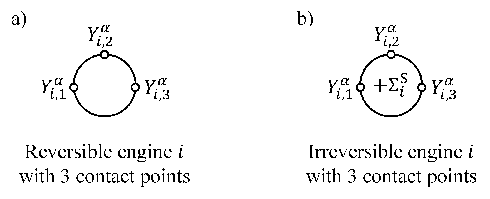
The notion of an engine refers to an energy conversion device, which operates either continuously or cyclically. We here consider continuously operating engines only. These have at least three contact points and are characterized by a set of algebraic balance equations for the extensities and energy:

$$\begin{array}{c}\hfill 0=\sum _r{J}_{i,r}^{\alpha },\end{array}$$

(7)

$$\begin{array}{c}\hfill 0=\sum _{r,\alpha }{I}_{i,r}^{\alpha }=\sum _{r,\alpha }{J}_{i,r}^{\alpha }{Y}_{i,r}^{\alpha }.\end{array}$$

(8)

As opposed to reservoirs, at the contact points of an engine, the intensities’ values generally differ so that all of these balance equations are fulfilled. This is an essential feature that allows engines to reversibly transfer energy between different intensity levels. As schematically shown in Figure 2a, engines are usually illustrated as circles.

A deviation from the standard notion of an endoreversible engine which will be made use of is an irreversible engine, where for ($\alpha =S$) Equation (7) is replaced by:

$$\begin{array}{c}\hfill 0=\sum _r{J}_{i,r}^{\mathrm{S}}+{\mathrm{\Sigma }}_i^{\mathrm{S}}\end{array}$$

(9)

with the entropy production rate ${\mathrm{\Sigma }}_i^{\mathrm{S}}$, which is included in Figure 2b to indicate irreversibility.

3. Interactions

Interactions describe transport phenomena and are the modeling objects to which, most often, all irreversibilities are confined in Endoreversible Thermodynamics. Therefore, a proper definition of the interactions is key to the validity of the model. Interactions can either be reversible or irreversible. In a reversible interaction, balance equations for energy and all conserved extensities, possibly including entropy, are required to hold. In contrast, in an irreversible interaction, balance equations must hold only for energy and all conserved extensities but not for entropy. Then, by a proper definition of transfer laws, it is guaranteed that entropy is either conserved or produced but never destroyed.

The number of contact points that an interaction attaches to is equal or larger than two. In the present paper, we will only consider bilateral interactions, that is, interactions that link exactly two contact points. The used symbolism pertaining to bilateral interactions is presented in Figure 3.

Reversible interactions are illustrated by straight arrows, whereas irreversible interactions are illustrated by wavy arrows. In the following, we will consider two essential examples of irreversible bilateral interactions that will be needed later.

First example: Heat conduction between two finite reservoirs is represented by an entropy flux carrying an energy flux (heat flux). The setup is schematically shown in Figure 4.

The energy flux may be modeled proportional to the temperature difference between the reservoirs, which corresponds to Newton’s law of heat transfer:

$$\begin{array}{c}\hfill -I_{1,1}^{\mathrm{S}}=I_{2,1}^{\mathrm{S}}:=K\left(T_1-T_2\right).\end{array}$$

(10)

Here, we have already stipulated energy conservation. If the heat conductance K is finite, then this is a resistive (or finite) transfer law, and the two temperatures may deviate significantly. Since $J_{i,r}^{\mathrm{S}}=I_{i,r}^{\mathrm{S}}/T_{i,r}$, it is obvious that the entropy fluxes at the two connected contact points will then have different magnitudes: The interaction is irreversible. The associated entropy production can be quantified as follows:

$$\begin{array}{c}\hfill {\mathrm{\Sigma }}^{\mathrm{S}}=J_{1,1}^{\mathrm{S}}+J_{2,1}^{\mathrm{S}}=K\left(\frac{T_1}{T_2}+\frac{T_2}{T_1}-2\right).\end{array}$$

(11)

Second example: We consider a pressure-driven flow of ideal gas directed from reservoir 1 to 2 as shown in Figure 5.

The gas flow is represented by a multi-extensity flux that consists of a particle flux $J_{i,r}^{\mathrm{n}}$ and a correlated entropy flux $J_{i,r}^{\mathrm{S}}$. The overall energy flux (enthalpy flux) carried by this multi-extensity flux is $I_{i,r}={\mu }_i{J}_{i,r}^{\mathrm{n}}+T_i{J}_{i,r}^{\mathrm{S}}$. We consider the flow direction where $J_{2,1}^{\mathrm{n}}>0$. Mass conservation and energy conservation read:

$$\begin{array}{c}\hfill 0=J_{1,1}^{\mathrm{n}}+J_{2,1}^{\mathrm{n}},\end{array}$$

(12)

$$\begin{array}{c}\hfill 0=I_{1,1}+I_{2,1}=J_{1,1}^{\mathrm{n}}{\mu }_1+J_{1,1}^{\mathrm{S}}{T}_1+I_{2,1}^{\mathrm{n}}{\mu }_2+I_{2,1}^{\mathrm{S}}{T}_2.\end{array}$$

(13)

For the transfer laws, we have:

$$\begin{array}{c}\hfill J_{1,1}^{\mathrm{n}}:=\gamma \left(p_2-p_1\right),\gamma >0,p_1>p_2\end{array}$$

(14)

$$\begin{array}{c}\hfill J_{1,1}^{\mathrm{S}}:=s(T_1,p_1)J_{1,1}^{\mathrm{n}},\end{array}$$

(15)

which are in accordance with $I_{1,1}:=c_{\mathrm{p}}{T}_1{J}_{1,1}^{\mathrm{n}}$. Entropy production then becomes:

$$\begin{array}{c}\hfill {\mathrm{\Sigma }}^{\mathrm{S}}={\dot{S}}_1+{\dot{S}}_2=J_{2,1}^{\mathrm{n}}\left[\underset{{\sigma }_{\mathrm{therm}}\ge 0}{\underbrace{c_{\mathrm{p}}\left(log\frac{T_2}{T_1}+\frac{T_1}{T_2}-1\right)}}+\underset{{\sigma }_{\mathrm{visc}}\ge 0}{\underbrace{Rlog\frac{p_1}{p_2}}}\right].\end{array}$$

(16)

Here, $\gamma >0$ is a particle transfer coefficient that is not necessarily constant but could, for instance, depend on $p_1$, $p_2$, $T_1$, and $T_2$. The first term in Equation (16) ${\sigma }_{\mathrm{therm}}$ concerns entropy production due to thermal mixing, whereas the second term ${\sigma }_{\mathrm{visc}}$ takes viscous dissipation into account. In the above equations, the expression:

$$\begin{array}{c}\hfill s(T,p)=c_{\mathrm{p}}log\frac{T}{T_{\mathrm{g}0}}-Rlog\frac{p}{p_{\mathrm{g}0}}+s_{\mathrm{g}0}\end{array}$$

(17)

for the ideal gas’ molar entropy has been used with the molar entropy $s_{\mathrm{g}0}$ at the reference conditions $T_{\mathrm{g}0}$, $p_{\mathrm{g}0}$, and the working gas’ isobaric molar heat capacity, $c_{\mathrm{p}}$. The corresponding entropy flux to subsystem 2 is:

$$\begin{array}{c}\hfill J_{2,1}^{\mathrm{S}}=\left(s(T_1,p_1)+\sigma \right)J_{2,1}^{\mathrm{n}}\end{array}$$

(18)

with the molar entropy production $\sigma :={\sigma }_{\mathrm{therm}}+{\sigma }_{\mathrm{visc}}$ according to Equation (16). It is revealing that the overall entropy production (Equation (16)) can, for the ideal gas, be expressed as consisting of two separate terms, each of which depends either only on temperatures or only on pressures and becomes zero if the respective temperatures or pressures are equal.

If one were to replace this interaction with a proper modeling object representing a thermal regenerator, one could expect it to diminish ${\sigma }_{\mathrm{therm}}$. Here, ${\sigma }_{\mathrm{therm}}=0$ would mean that the temperature of the gas leaving the regenerator was equal to $T_2$ and the regenerator compensated for the current surplus or deficit of $(I_{1,1}+I_{2,1})$ and $(J_{1,1}^{\mathrm{S}}+J_{2,1}^{\mathrm{S}})$. Moreover, ${\sigma }_{\mathrm{visc}}$ would be zero if a non-resistive particle transfer law resulting in $p_1/p_2=1$ was considered. On the other hand, if one considers a resistive (or finite) particle transfer law resulting in $p_1/p_2>1$, then the viscous molar entropy production ${\sigma }_{\mathrm{visc}}$ would be grater than zero.

4. Endoreversible Regenerator Modeling

As mentioned above, the endoreversible subsystems that will be used to construct the internal structure of the endoreversible regenerator model are reservoirs, on the one hand, and engines without extensity buffers on the other. A thermal regenerator is neither a reservoir nor such an engine since it encompasses features of both: It contains extensities and energy, and it has contact points with differing intensities. It may, hence, be properly represented by some combination of both kinds of subsystems. In this section, we will develop three variants of an endoreversible regenerator model, which we will refer to as $\mathit{ES}$-regenerator, $\mathit{EE}$-regenerator, and $\mathit{EEn}$-regenerator models.

4.1. $ES$-Regenerator Model

For the purpose of the description of the $ES$-regenerator model, the regenerator’s internal endoreversible structure will be neglected. It will be considered only as a black box for which the first and second law are required to hold. The model is motivated by the notion of an internally reversible regenerator, which conserves both energy E and entropy S, and correspondingly has zero internal entropy production: ${\mathrm{\Sigma }}_{\mathrm{R}}^{\mathrm{S}}=0$. Nevertheless, the model is technically not limited to the ideal description. In fact, the entropy production term ${\mathrm{\Sigma }}_{\mathrm{R}}^{\mathrm{S}}$ will be included in the entropy balance equation as a placeholder. The $\mathit{ES}$-regenerator model is based on the following modeling assumptions:

(A)

Only operational conditions are considered in which the local temperature difference between the regenerator matrix, and working gas is small so that it can be neglected when determining the temperatures of the working gas flowing out of the regenerator on its hot and cold side. Thus, the contact point temperatures can be defined as equal to the matrix temperature of the respective regenerator side.

(B)

The temperature distribution in the regenerator matrix is linear at all times, and the sign of its gradient is uniquely determined by the boundary conditions. Hence, the state of the regenerator matrix features two degrees of freedom. In the $\mathit{ES}$-regenerator model, the state is specified by providing the energy E and entropy S contained in the matrix.

(C)

Only the regenerator matrix and its interactions with the working gas are encompassed by the $\mathit{ES}$-regenerator model. That is, the regenerator model itself does not feature a dead volume. The influence of the regenerator dead volume may be taken into account approximately by allocating it to the adjacent gas reservoirs.

Assumption (B) which regards the linearity of the temperature profile is not valid under arbitrary (transient) operational conditions of regenerators. It may, however, be an appropriate approximation for the stationary operational state that the regenerator approaches after many cycles under typical stationary operational conditions. This (periodic) stationary operational state is what the model is intended to describe.

We will strictly distinguish between internal irreversibilities ${\mathrm{\Sigma }}_{\mathrm{R}}^{\mathrm{S}}$ that are associated with loss phenomena occurring inside the regenerator and external irreversibilities that occur in the interactions of the regenerator with the adjacent subsystems. The internal irreversibilities ${\mathrm{\Sigma }}_{\mathrm{R}}^{\mathrm{S}}$ can be set to zero or can alternatively be defined via other submodels as introduced later, whereas the external irreversibilities are not arbitrarily definable. The external irreversibilities rather result from the exchanged particle fluxes and temperatures at the contact points of the regenerator and the adjacent gas reservoirs.

The particle flux through the regenerator is modeled as driven by the pressure difference between the regenerator’s hot and cold side. A particle flux, in turn, induces an entropy flux. This means a gas flow is described as a multi-extensity flux of particles and entropy. Inflows and outflows of gas on the regenerator’s hot and cold side are considered to take place at the pressure of the gas reservoir that the respective regenerator contact point is connected to. However, as depicted in Figure 6, temperature differences between gas reservoir and regenerator can occur. As this constitutes a bilateral interaction of subsystems that are not necessarily in thermal equilibrium, these temperature differences result in entropy production according to Equation (16). Therefore, the external irreversibility generally occurs even if the regenerator is internally fully reversible.

4.1.1. Contact Point Temperatures as Functions of State Variables

In what follows, the expressions for the regenerator’s energy and entropy are derived as functions of the linear temperature distribution between the two contact point temperatures $T_{\mathrm{R},\mathrm{H}}$ and $T_{\mathrm{R},\mathrm{L}}$ of the regenerator. The energy and entropy expressions will afterwards be inverted to obtain expressions for the contact point temperatures as functions of energy and entropy. These temperature expressions will later on be needed to determine energy fluxes and entropy fluxes to and from the adjacent gas reservoirs.

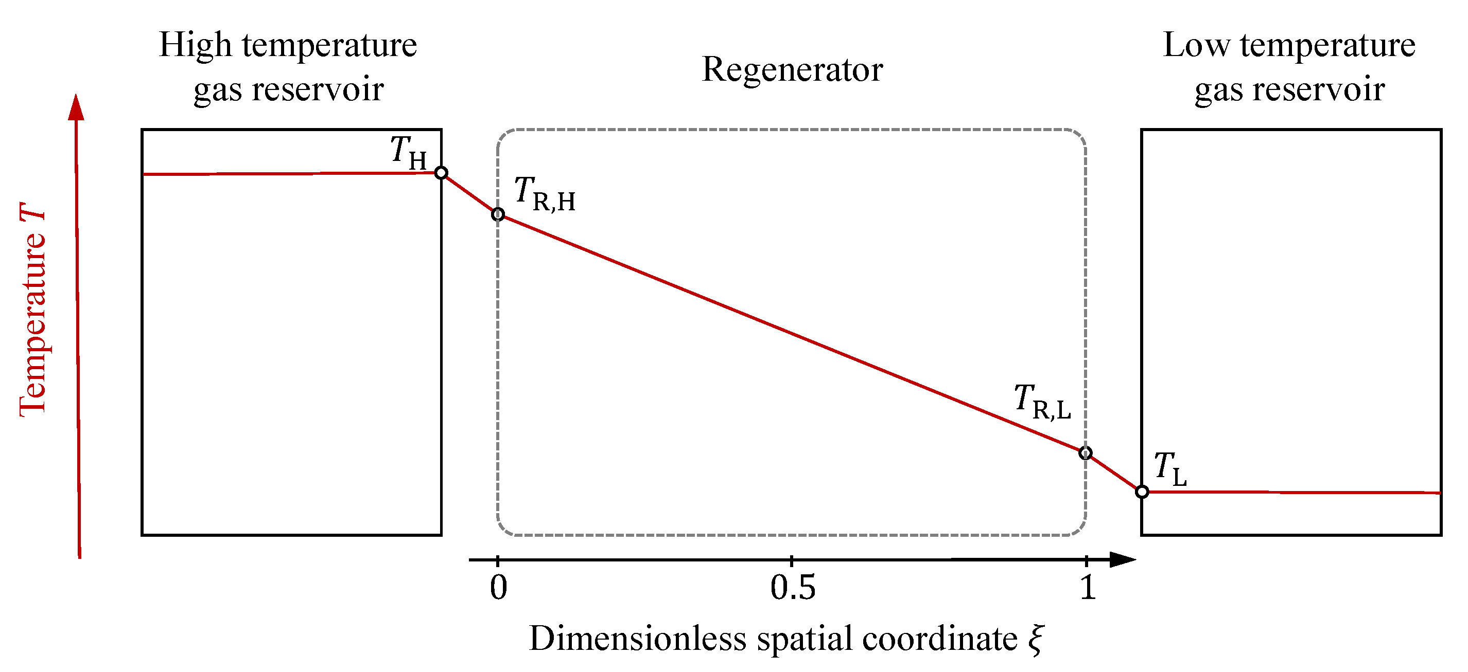
The expressions for energy and entropy are obtained by considering the regenerator as a one-dimensional continuum, as schematically shown in Figure 6. The specific energy (energy per mass unit) at some point $\xi$ in this continuum is defined as:

$$\begin{array}{c}\hfill e_{\mathrm{R}}\left(\xi \right):=c_{\mathrm{R}}{T}_{\mathrm{R}}\left(\xi \right)\end{array}$$

(19)

with the matrix material’s specific heat capacity $c_{\mathrm{R}}$ and the temperature $T_{\mathrm{R}}\left(\xi \right)$. The specific entropy (entropy per mass unit) is:

$$\begin{array}{c}\hfill s_{\mathrm{R}}\left(\xi \right):=c_{\mathrm{R}}log\frac{T_{\mathrm{R}}\left(\xi \right)}{T_{\mathrm{R}0}}+s_{\mathrm{R}0}\end{array}$$

(20)

where $s_{\mathrm{R}0}$ is the specific entropy at the reference temperature $T_{\mathrm{R}0}$. We assume that the temperature profile in the regenerator is linear at all times. That is, it takes the form:

$$\begin{array}{c}\hfill T_{\mathrm{R}}\left(\xi \right):=T_{\mathrm{R},\mathrm{H}}+\xi \left(T_{\mathrm{R},\mathrm{L}}-T_{\mathrm{R},\mathrm{H}}\right)\end{array}$$

(21)

with the dimensionless coordinate $\xi \in [0,1]$ and the contact point temperatures $T_{\mathrm{R},\mathrm{H}}>T_{\mathrm{R},\mathrm{L}}$ as depicted in Figure 6. For homogeneous mass density ${\rho }_{\mathrm{R}}$ and homogenous specific heat capacity $c_{\mathrm{R}}$, the energy of the regenerator becomes:

$$\begin{array}{c}\hfill E_{\mathrm{R}}(T_{\mathrm{R},\mathrm{H}},T_{\mathrm{R},\mathrm{L}})=m_{\mathrm{R}}{\int }_0^1{e}_{\mathrm{R}}\left(\xi \right)\mathrm{d}\xi =C_{\mathrm{R}}\frac{T_{\mathrm{R},\mathrm{L}}+T_{\mathrm{R},\mathrm{H}}}{2}\end{array}$$

(22)

with the mass $m_{\mathrm{R}}$ and the overall heat capacity $C_{\mathrm{R}}=m_{\mathrm{R}}{c}_{\mathrm{R}}$ of the regenerator matrix. Analogously, the entropy of the regenerator matrix becomes:

$$\begin{array}{c}\hfill \begin{array}{cc}\hfill S_{\mathrm{R}}(T_{\mathrm{R},\mathrm{H}},T_{\mathrm{R},\mathrm{L}})& =m_{\mathrm{R}}{\int }_0^1{s}_{\mathrm{R}}\left(\xi \right)\mathrm{d}\xi \hfill \\ \hfill & =C_{\mathrm{R}}\left(\frac{T_{\mathrm{R},\mathrm{L}}}{T_{\mathrm{R},\mathrm{H}}-T_{\mathrm{R},\mathrm{L}}}log\frac{T_{\mathrm{R},\mathrm{H}}}{T_{\mathrm{R},\mathrm{L}}}+log\frac{T_{\mathrm{R},\mathrm{H}}}{T_{\mathrm{R}0}}-1\right)+S_{\mathrm{R}0}\hfill \end{array}\end{array}$$

(23)

where $S_{\mathrm{R}0}=m_{\mathrm{R}}{s}_{\mathrm{R}0}$ is the regenerator’s entropy at the reference temperature $T_{\mathrm{R}0}$. Under the strict condition $T_{\mathrm{R},\mathrm{H}}>T_{\mathrm{R},\mathrm{L}}$ and the linear temperature profile requirement, the sets $\left\{T_{\mathrm{R},\mathrm{H}},T_{\mathrm{R},\mathrm{L}}\right\}$ and $\left\{E_{\mathrm{R}},S_{\mathrm{R}}\right\}$ are bijective. That is, the temperatures $T_{\mathrm{R},\mathrm{H}}$ and $T_{\mathrm{R},\mathrm{L}}$ can be expressed as unique functions of $E_{\mathrm{R}}$ and $S_{\mathrm{R}}$.

However, inverting Equations (22) and (23) is not practicable analytically. Therefore, the entropy expression is approximated. For this purpose, we define the mean temperature $T_{\mathrm{R}}^{\mathrm{M}}:=(T_{\mathrm{R},\mathrm{H}}+T_{\mathrm{R},\mathrm{L}})/2$ and the temperature difference $T_{\mathrm{R}}^{\Delta }:=T_{\mathrm{R},\mathrm{H}}-T_{\mathrm{R},\mathrm{L}}$. Using the fourth order Taylor expansion of $S_{\mathrm{R}}$ as a function of the temperature difference $T_{\mathrm{R}}^{\Delta }$ around $T_{\mathrm{R}}^{\Delta }=0$ yields:

$$\begin{array}{c}\hfill S_{\mathrm{R}}(T_{\mathrm{R},\mathrm{H}},T_{\mathrm{R},\mathrm{L}})\approx S_{\mathrm{R}0}+C_{\mathrm{R}}log\frac{T_{\mathrm{R}}^{\mathrm{M}}}{T_{\mathrm{R}0}}-\frac{C_{\mathrm{R}}}{24}{\left(\frac{T_{\mathrm{R}}^{\Delta }}{T_{\mathrm{R}}^{\mathrm{M}}}\right)}^2-\frac{C_{\mathrm{R}}}{320}{\left(\frac{T_{\mathrm{R}}^{\Delta }}{T_{\mathrm{R}}^{\mathrm{M}}}\right)}^4.\end{array}$$

(24)

The corresponding approximative expressions for $T_{\mathrm{R},\mathrm{H}}$ and $T_{\mathrm{R},\mathrm{L}}$ are:

$$\begin{array}{c}\hfill T_{\mathrm{R},\mathrm{H}}(E_{\mathrm{R}},S_{\mathrm{R}}):=\frac{E_{\mathrm{R}}}{C_{\mathrm{R}}}\left(1+\sqrt{-\frac{5}{3}+\sqrt{\frac{25}{9}+20\left(\frac{S_{\mathrm{R}0}-S_{\mathrm{R}}}{C_{\mathrm{R}}}+log\frac{E_{\mathrm{R}}}{C_{\mathrm{R}}{T}_{\mathrm{R}0}}\right)}}\right),\end{array}$$

(25)

$$\begin{array}{c}\hfill T_{\mathrm{R},\mathrm{L}}(E_{\mathrm{R}},S_{\mathrm{R}}):=\frac{E_{\mathrm{R}}}{C_{\mathrm{R}}}\left(1-\sqrt{-\frac{5}{3}+\sqrt{\frac{25}{9}+20\left(\frac{S_{\mathrm{R}0}-S_{\mathrm{R}}}{C_{\mathrm{R}}}+log\frac{E_{\mathrm{R}}}{C_{\mathrm{R}}{T}_{\mathrm{R}0}}\right)}}\right).\end{array}$$

(26)

Note, this definition of $T_{\mathrm{R},\mathrm{H}}$ and $T_{\mathrm{R},\mathrm{L}}$ required additional knowledge about the sign of the temperature gradient, which we provided by stating $T_{\mathrm{R},\mathrm{H}}>T_{\mathrm{R},\mathrm{L}}$. This limitation of the $\mathit{ES}$-regenerator model can be overcome by introducing an internal endoreversible structure, as will be conducted in Section 4.2.

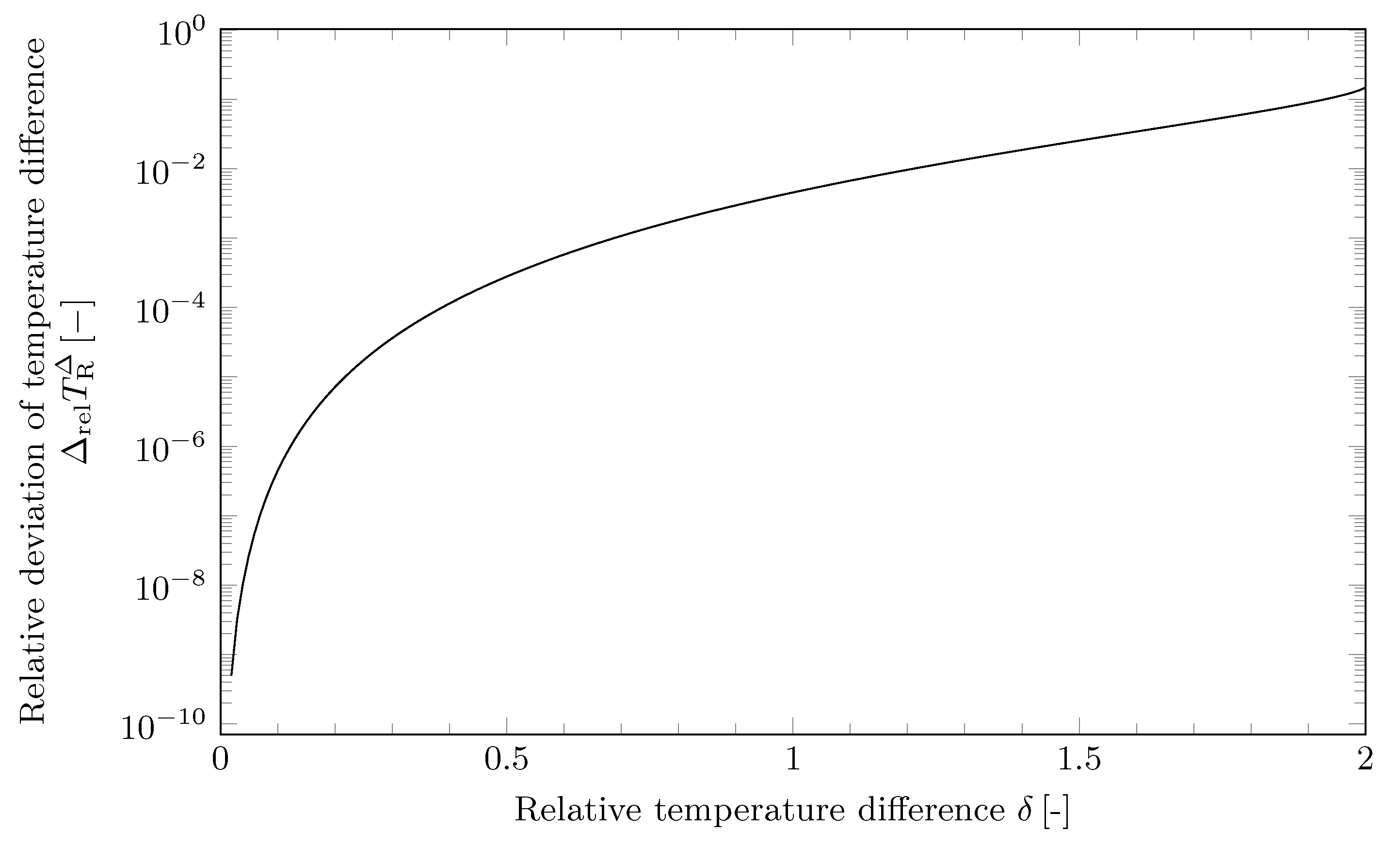
The approximative expressions of Equations (25) and (26) do not entail a deviation from the exact solution in the mean temperature $T_{\mathrm{R}}^{\mathrm{M}}$ since the mean temperature is in either case $E_{\mathrm{R}}/C_{\mathrm{R}}$. However, in the temperature difference $T_{\mathrm{R}}^{\Delta }$, a deviation occurs, which can be determined via:

$$\begin{array}{c}\hfill \begin{array}{cc}\hfill {\Delta }_{\mathrm{rel}}{T}_{\mathrm{R}}^{\Delta }(T_1,T_2):=& \frac{T_{\mathrm{R},\mathrm{H}}(E_{\mathrm{R}}(T_1,T_2),S_{\mathrm{R}}(T_1,T_2))-T_{\mathrm{R},\mathrm{L}}(E_{\mathrm{R}}(T_1,T_2),S_{\mathrm{R}}(T_1,T_2))}{T_1-T_2}-1\hfill \\ \hfill =& \frac{T_1+T_2}{T_1-T_2}\sqrt{-\frac{5}{3}+\sqrt{\frac{205}{9}+20\left(\frac{T_2}{T_1-T_2}log\frac{T_2}{T_1}+log\frac{T_1+T_2}{2T_1}\right)}}-1.\hfill \end{array}\end{array}$$

(27)

Here, $T_1>T_2$ represent predefined contact point temperatures, and the entropy is calculated according to Equation (23). Note that Equation (27) solely depends on the temperatures. The relative deviation ${\Delta }_{\mathrm{rel}}{T}_{\mathrm{R}}^{\Delta }$ can also be expressed as a function of the relative temperature difference $\delta :=2(T_1-T_2)/(T_1+T_2)$:

$$\begin{array}{c}\hfill \begin{array}{cc}\hfill & {\Delta }_{\mathrm{rel}}{T}_{\mathrm{R}}^{\Delta }\left(\delta \right)=\hfill \\ \hfill & \frac{2}{\delta }\sqrt{-\frac{5}{3}+\sqrt{\frac{205}{9}+20\left(\left(\frac{1}{\delta }-\frac{1}{2}\right)log\left(\frac{2}{\delta +2}-\frac{1}{2/\delta +1}\right)-log\left(1+\frac{\delta }{2}\right)\right)}}-1.\hfill \end{array}\end{array}$$

(28)

This function is plotted in Figure 7.

It can be observed that the relative deviation of the temperature difference introduced by the approximation from Equation (24) is smaller than $3\times {10}^{-4}$ for a relative temperature difference $\delta \le 0.5$. For a relative temperature difference of $\delta \le 1.4$, the relative deviation is still smaller than $2\times {10}^{-2}$. Since this is assumed to hold in a broad range of model situations, the deviations entailed in Equations (25) and (26) are regarded as negligible.

4.1.2. Regenerator State Dynamics

In Figure 8a, a schematics of the $\mathit{ES}$-regenerator model is shown. The straight arrows depict reversible fluxes, and the wavy arrows depict irreversible fluxes. The state of the regenerator is determined by $E_{\mathrm{R}}$ and $S_{\mathrm{R}}$, which obey the balance laws:

$$\begin{array}{c}\hfill {\dot{E}}_{\mathrm{R}}=I_{\mathrm{R},\mathrm{H}}+I_{\mathrm{R},\mathrm{L}},\end{array}$$

(29)

$$\begin{array}{c}\hfill {\dot{S}}_{\mathrm{R}}=J_{\mathrm{R},\mathrm{H}}^{\mathrm{S}}+J_{\mathrm{R},\mathrm{L}}^{\mathrm{S}}+{\mathrm{\Sigma }}_{\mathrm{R}}^{\mathrm{S}}.\end{array}$$

(30)

Here, $J_{\mathrm{R},\mathrm{H}}^{\mathrm{S}}$ and $J_{\mathrm{R},\mathrm{L}}^{\mathrm{S}}$ are entropy fluxes entering the regenerator at the contact points H and L. Together with the particle fluxes $J_{\mathrm{R},\mathrm{H}}^{\mathrm{n}}$ and $J_{\mathrm{R},\mathrm{L}}^{\mathrm{n}}$, they carry the energy fluxes $I_{\mathrm{R},\mathrm{H}}$ and $I_{\mathrm{R},\mathrm{L}}$, respectively. Furthermore, ${\mathrm{\Sigma }}_{\mathrm{R}}^{\mathrm{S}}$ is the sum of all internal entropy sources which can for now taken to be zero (internally reversible regenerator). It is the placeholder for internal irreversibilities that will be addressed in Section 5.

Inflows and outflows of working gas are considered to occur without pressure differences between the a regenerator contact point and the respective gas reservoir $i\in \left\{\mathrm{H},\mathrm{L}\right\}$. Correspondingly, for inflows of working gas, the energy flux and entropy flux are determined from the gas reservoir’s temperature $T_i$ and pressure $p_i$ as well as the respective regenerator contact point temperature $T_{\mathrm{R},i}$:

$$\begin{array}{c}\hfill I_{\mathrm{R},i}=c_{\mathrm{p}}{T}_i{J}_{\mathrm{R},i}^{\mathrm{n}},\end{array}$$

(31)

$$\begin{array}{c}\hfill J_{\mathrm{R},i}^{\mathrm{S}}=\left(s(T_i,p_i)+\sigma (T_i,T_{\mathrm{R},i})\right)J_{\mathrm{R},i}^{\mathrm{n}}.\end{array}$$

(32)

Entropy production, which is due to the temperature difference between the gas reservoir and the regenerator contact point, is here taken into account with:

$$\begin{array}{c}\hfill \sigma (T_i,T_{\mathrm{R},i}):=c_{\mathrm{p}}\left(log\frac{T_{\mathrm{R},i}}{T_i}+\frac{T_i}{T_{\mathrm{R},i}}-1\right).\end{array}$$

(33)

As opposed to that, for outflows of working gas, the fluxes of energy and entropy at the regenerator’s contact point are determined as:

$$\begin{array}{c}\hfill I_{\mathrm{R},i}=c_{\mathrm{p}}{T}_{\mathrm{R},i}{J}_{\mathrm{R},i}^{\mathrm{n}},\end{array}$$

(34)

$$\begin{array}{c}\hfill J_{\mathrm{R},i}^{\mathrm{S}}=s(T_{\mathrm{R},i},p_i)J_{\mathrm{R},i}^{\mathrm{n}}\end{array}$$

(35)

according to the respective contact point temperature (Equations (25) or (26)). Since this contact point temperature generally differs from the temperature $T_i$ inside the gas reservoir, the interaction is also irreversible in this flow direction.

In order to show the principle behavior of the $\mathit{ES}$-regenerator model, we consider a setup as illustrated in Figure 8 where the temperatures of the adjacent gas reservoirs are maintained at $T_{\mathrm{H}}=500$ K and $T_{\mathrm{L}}=300$ K, and their pressures are maintained at $p_{\mathrm{H}}=p_{\mathrm{L}}=50$ bar. This corresponds to a reduced pressure $p/p_{\mathrm{crit}}$ of ca. 22, which is rather high for the application of the ideal gas law. Nevertheless, we chose this high pressure value as it helps to illustrate the general behavior of the models developed, in particular the influence of pressure oscillations in the EEn-regenerator model is presented below. Depending on the accuracy required in a certain application, it might be necessary to use a constitutive law other than the ideal gas law. This would require an extension of the models presented here, involving the adaptions of Equation (3) and all the equations based thereon, for example, Equations (16), (17), and (33). This, however, is beyond the scope of the current paper. The particle transfer through the regenerator shall obey a non-resistive transfer law ($\gamma \to \infty$) with the particle flux $J_{\mathrm{R},\mathrm{H}}^{\mathrm{n}}$ prescribed as a sinusoidal function with a cycle time of $\tau =0.1$ s and an amplitude of 10 mol/s. The working gas shall be helium [47]. The regenerator is considered as internally reversible (${\mathrm{\Sigma }}_{\mathrm{R}}^{\mathrm{S}}:=0$), and its heat capacity is 300 J/K.

For these parameters, the dynamics of the $\mathit{ES}$-regenerator model was integrated until a cyclic operational state was achieved. In Figure 9, the calculated contact point temperatures $T_{\mathrm{R},\mathrm{H}}$ and $T_{\mathrm{R},\mathrm{L}}$ are plotted as solid lines, and the gas reservoir temperatures $T_{\mathrm{H}}$ and $T_{\mathrm{L}}$ are plotted as dotted lines.

Additionally, to provide a benchmark, in Figure 9, the results of a finite volume regenerator model using 200 regenerator layers are plotted with dashed lines. Each of those layers consists of a gas reservoir, which represents a slice of the regenerator dead space (measuring $0.8$ L in total) and is linked by a non-resistive-heat-transfer interaction to a dedicated heat reservoir representing the respective slice of the matrix. Correspondingly, $T_{\mathrm{R},\mathrm{H}}^{\mathrm{FVM}}$ and $T_{\mathrm{R},\mathrm{L}}^{\mathrm{FVM}}$ are the temperatures of the two outermost slices that are connected to the adjacent gas reservoirs H and L.

In Figure 9, it can be observed that the regenerator contact point temperatures of the $\mathit{ES}$-regenerator model oscillate around the constant temperatures $T_{\mathrm{H}}$ and $T_{\mathrm{L}}$ of the adjacent gas reservoirs with approximately harmonic shapes. This means that $T_{\mathrm{R},\mathrm{H}}$ overshoots $T_{\mathrm{H}}$ and $T_{\mathrm{R},\mathrm{L}}$ undershoots $T_{\mathrm{L}}$. As opposed to that, the shapes of the contact point temperature curves predicted by the finite volume model deviate from harmonic shapes so that $T_{\mathrm{R},\mathrm{H}}^{\mathrm{FVM}}$ does not proceed above $T_{\mathrm{H}}$, and $T_{\mathrm{R},\mathrm{L}}^{\mathrm{FVM}}$ does not proceed below $T_{\mathrm{L}}$. It is obvious that this is a more realistic description of the behavior of a real regenerator. It is connected to slight deviations from a linear temperature profile in the finite volume model, which are not described by the $\mathit{ES}$-regenerator model.

Nevertheless, the temperature deviations $T_{\mathrm{R},i}-T_{\mathrm{R},i}^{\mathrm{FVM}}$ ($i\in \left\{\mathrm{H},\mathrm{L}\right\}$) are relatively small compared to the temperature difference $T_{\mathrm{H}}-T_{\mathrm{L}}$. This is particularly remarkable in the light of the significantly lower numerical effort involved by the $\mathit{ES}$-regenerator model. Moreover, it is important to note that a real regenerator cannot operate internally reversible, which means ${\mathrm{\Sigma }}_{\mathrm{R}}^{\mathrm{S}}>0$. Due to these internal irreversibilities, the regenerator contact point temperatures will approach each other, and the cutoffs by $T_{\mathrm{H}}$ and $T_{\mathrm{L}}$ will become less dominant. Hence, as long as ${\mathrm{\Sigma }}_{\mathrm{R}}^{\mathrm{S}}$ is modeled properly as an input for the $\mathit{ES}$-regenerator model, it can be expected that the latter model provides good approximations for the regenerator contact point temperatures.

4.2. $\mathit{EE}$-Regenerator Model

In the $\mathit{ES}$-regenerator model introduced in the previous section, the regenerator’s internal endoreversible structure was neglected, and the regenerator’s overall energy and entropy content served to identify its state. The requirements of conservation of energy and entropy within the subsystem boundaries of the regenerator provided its state dynamics via the state variables energy and entropy.

The two degrees of freedom of the endoreversible regenerator can also be expressed using different state variables. These are in the following defined via the internal endoreversible structure shown in Figure 10.

It consists of an engine (where ${\mathrm{\Sigma }}_{\mathrm{R}}^{\mathrm{S}}$ is again the placeholder for internal irreversibilities, which can for now taken to be zero) and two heat reservoirs that have the heat capacities $C_{\mathrm{R}.\mathrm{h}}:=C_{\mathrm{R}.\mathrm{l}}:=C_{\mathrm{R}}/2$ and the independent energies $E_{\mathrm{R}.\mathrm{h}}$ and $E_{\mathrm{R}.\mathrm{l}}$. Each of the two internal heat reservoirs features one degree of freedom. Correspondingly, in the $\mathit{EE}$-regenerator model, the two internal heat reservoirs’ energies are taken as state variables of the regenerator. Given the energies, the entropies of the internal heat reservoirs can be calculated as:

$$\begin{array}{c}\hfill S_{\mathrm{R}.\mathrm{h}}:=C_{\mathrm{R}.\mathrm{h}}log\frac{E_{\mathrm{R}.\mathrm{h}}}{C_{\mathrm{R}.\mathrm{h}}{T}_{\mathrm{R}0}}+\frac{S_{\mathrm{R}0}}{2},\end{array}$$

(36)

$$\begin{array}{c}\hfill S_{\mathrm{R}.\mathrm{l}}:=C_{\mathrm{R}.\mathrm{l}}log\frac{E_{\mathrm{R}.\mathrm{l}}}{C_{\mathrm{R}.\mathrm{l}}{T}_{\mathrm{R}0}}+\frac{S_{\mathrm{R}0}}{2}.\end{array}$$

(37)

With $E_{\mathrm{R}}=E_{\mathrm{R}.\mathrm{h}}+E_{\mathrm{R}.\mathrm{l}}$ and $S_{\mathrm{R}}=S_{\mathrm{R}.\mathrm{h}}+S_{\mathrm{R}.\mathrm{l}}$, these expressions can be inserted into Equations (25) and (26). Furthermore, the sign of the temperature gradient can be identified with the sign of the difference of the energies $E_{\mathrm{R}.\mathrm{h}}$ and $E_{\mathrm{R}.\mathrm{l}}$:

$$\begin{array}{c}\hfill T_{\mathrm{R},\mathrm{H}}:=\frac{E_{\mathrm{R}.\mathrm{h}}+E_{\mathrm{R}.\mathrm{l}}}{C_{\mathrm{R}}}\left(1+\mathrm{sign}\left(E_{\mathrm{R}.\mathrm{h}}-E_{\mathrm{R}.\mathrm{l}}\right)\sqrt{-\frac{5}{3}+\sqrt{\frac{25}{9}+20log\frac{E_{\mathrm{R}.\mathrm{h}}+E_{\mathrm{R}.\mathrm{l}}}{2\sqrt{E_{\mathrm{R}.\mathrm{h}}{E}_{\mathrm{R}.\mathrm{l}}}}}}\right),\end{array}$$

(38)

$$\begin{array}{c}\hfill T_{\mathrm{R},\mathrm{L}}:=\frac{E_{\mathrm{R}.\mathrm{h}}+E_{\mathrm{R}.\mathrm{l}}}{C_{\mathrm{R}}}\left(1-\mathrm{sign}\left(E_{\mathrm{R}.\mathrm{h}}-E_{\mathrm{R}.\mathrm{l}}\right)\sqrt{-\frac{5}{3}+\sqrt{\frac{25}{9}+20log\frac{E_{\mathrm{R}.\mathrm{h}}+E_{\mathrm{R}.\mathrm{l}}}{2\sqrt{E_{\mathrm{R}.\mathrm{h}}{E}_{\mathrm{R}.\mathrm{l}}}}}}\right).\end{array}$$

(39)

From the engine’s balance equations for energy and entropy, the dynamics of the two heat reservoirs follows:

$$\begin{array}{c}\hfill {\dot{E}}_{\mathrm{R}.\mathrm{h}}=\begin{array}{c}\hfill I_{\mathrm{R}.\mathrm{h}}^{\mathrm{S}}\end{array}=I_{\mathrm{R},\mathrm{H}}-I_{\mathrm{R}.\mathrm{hl}},\end{array}$$

(40)

$$\begin{array}{c}\hfill {\dot{E}}_{\mathrm{R}.\mathrm{l}}=\begin{array}{c}\hfill I_{\mathrm{R}.\mathrm{l}}^{\mathrm{S}}\end{array}=I_{\mathrm{R},\mathrm{L}}+I_{\mathrm{R}.\mathrm{hl}},\end{array}$$

(41)

with the auxiliary energy flux $I_{\mathrm{R}.\mathrm{hl}}$, which the two internal heat reservoirs exchange through the engine as part of $I_{\mathrm{R}.\mathrm{h}}^{\mathrm{S}}$ and $I_{\mathrm{R}.\mathrm{l}}^{\mathrm{S}}$:

$$\begin{array}{c}\hfill I_{\mathrm{R}.\mathrm{hl}}=\frac{\frac{2}{C_{\mathrm{R}}}\left(J_{\mathrm{R},\mathrm{H}}^{\mathrm{S}}+J_{\mathrm{R},\mathrm{L}}^{\mathrm{S}}+{\mathrm{\Sigma }}_{\mathrm{R}}^{\mathrm{S}}\right)-\frac{I_{\mathrm{R},\mathrm{H}}}{E_{\mathrm{R}.\mathrm{h}}}-\frac{I_{\mathrm{R},\mathrm{L}}}{E_{\mathrm{R}.\mathrm{l}}}}{1/E_{\mathrm{R}.\mathrm{l}}-1/E_{\mathrm{R}.\mathrm{h}}}.\end{array}$$

(42)

This auxiliary energy flux is a measure of the rate of change of the temperature difference ${\dot{T}}_{\mathrm{R}}^{\Delta }$ that is necessary for the regenerator to take up or release entropy as prescribed by the external interactions and the internal source term ${\mathrm{\Sigma }}_{\mathrm{R}}^{\mathrm{S}}$. Note that the denominator of Equation (42) tends to zero if the energy difference $(E_{\mathrm{R}.\mathrm{h}}-E_{\mathrm{R}.\mathrm{l}})\to 0$. Then, also the difference of the contact point temperatures $T_{\mathrm{R}}^{\Delta }\to 0$ and, therefore, $\partial S_{\mathrm{R}}/\partial T_{\mathrm{R}}^{\Delta }\to 0$. Let us consider the case in which the energy of the regenerator stays constant while the entropy changes: ${\dot{T}}_{\mathrm{R}}^{\Delta }{|}_{E_{\mathrm{R}}}=\partial T_{\mathrm{R}}^{\Delta }/\partial S_{\mathrm{R}}{\dot{S}}_{\mathrm{R}}$. Hence, $|{\dot{T}}_{\mathrm{R}}^{\Delta }|\to \infty$ for finite ${\dot{S}}_{\mathrm{R}}$, which is consistent with $|I_{\mathrm{R}.\mathrm{hl}}|\to \infty$. In order to obtain a numerically stable algorithm, it is necessary to limit $I_{\mathrm{R}.\mathrm{hl}}$ in a small region $|E_{\mathrm{R}.\mathrm{h}}-E_{\mathrm{R}.\mathrm{l}}|<\epsilon$. Consequently, the entropy conservation equation is not fulfilled in the region below $\epsilon$. However, since thermal regenerators are usually not operated in a way such that zero-crossings of the temperature gradient occur during the cycle, this is of no significance for the steady-state cyclic operation of the regenerator with a proper choice of $\epsilon$.

Since the definitions of the contact point temperatures $T_{\mathrm{R},\mathrm{H}}$ and $T_{\mathrm{R},\mathrm{L}}$ from Equations (38) and (39) are made dependent on the sign of $E_{\mathrm{R}.\mathrm{h}}-E_{\mathrm{R}.\mathrm{l}}$, the $\mathit{EE}$-regenerator model is capable of describing temporal evolutions of $T_{\mathrm{R},\mathrm{H}}$ and $T_{\mathrm{R},\mathrm{L}}$ that involve sign changes of the regenerator’s temperature gradient. This was not possible in the $\mathit{ES}$-regenerator model, where the sign of the temperature gradient was predefined. Apart from that, the dynamical behavior of the two models is identical so that the results of the $\mathit{EE}$-regenerator model are equal to those shown in Figure 9.

4.3. $\mathit{EEn}$-Regenerator Model

Model assumption (C) results in a more drastic simplification that separates the treatment of regeneration itself from the description of the influence of the regenerator dead volume. In doing so, the number of degrees of freedom of the regenerator is kept minimal. However, the presented $\mathit{EE}$-regenerator model can be extended by adding a gas reservoir R.d, for which its temperature $T_{\mathrm{R}.\mathrm{d}}$ is maintained at the logarithmic mean temperature of the two contact point temperatures:

$$\begin{array}{c}\hfill \begin{array}{c}\hfill {\tilde{T}}_{\mathrm{R},\mathrm{H},\mathrm{L}}=\frac{T_{\mathrm{R},\mathrm{H}}-T_{\mathrm{R},\mathrm{L}}}{\log \left(T_{\mathrm{R},\mathrm{H}}\right)-\log \left(T_{\mathrm{R},\mathrm{L}}\right)}.\end{array}\end{array}$$

(43)

Its volume $V_{\mathrm{R}.\mathrm{d}}$ shall correspond to the regenerator’s dead volume. Then, its pressure $p_{\mathrm{R}.\mathrm{d}}$ results from ${\tilde{T}}_{\mathrm{R},\mathrm{H},\mathrm{L}}$, $V_{\mathrm{R}.\mathrm{d}}$ and the particle number $n_{\mathrm{R}.\mathrm{d}}$ contained in the regenerator dead space. The correspondingly extended $\mathit{EEn}$-regenerator model [49] features three degrees of freedom and is schematically shown in Figure 11.

The definition of contact point temperatures can be taken from the $\mathit{EE}$-regenerator model. The regenerator dynamics, however, needs to be adapted to account for extensity and energy transfers with the internal gas reservoir:

$$\begin{array}{c}\hfill {\dot{E}}_{\mathrm{R}.\mathrm{h}}=I_{\mathrm{R}.\mathrm{h}}=I_{\mathrm{R},\mathrm{H}}-I_{\mathrm{R}.\mathrm{hl}}-I_{\mathrm{R}.\mathrm{d}}/2,\end{array}$$

(44)

$$\begin{array}{c}\hfill {\dot{E}}_{\mathrm{R}.\mathrm{l}}=I_{\mathrm{R}.\mathrm{l}}=I_{\mathrm{R},\mathrm{L}}+I_{\mathrm{R}.\mathrm{hl}}-I_{\mathrm{R}.\mathrm{d}}/2,\end{array}$$

(45)

$$\begin{array}{c}\hfill {\dot{n}}_{\mathrm{R}.\mathrm{d}}=J_{\mathrm{R}.\mathrm{d}}^{\mathrm{n}}=J_{\mathrm{R},\mathrm{H}}^{\mathrm{n}}+J_{\mathrm{R},\mathrm{L}}^{\mathrm{n}},\end{array}$$

(46)

with the auxiliary energy flux now being:

$$\begin{array}{c}\hfill I_{\mathrm{R}.\mathrm{hl}}=\frac{\frac{2}{C_{\mathrm{R}}}\left(J_{\mathrm{R},\mathrm{H}}^{\mathrm{S}}+J_{\mathrm{R},\mathrm{L}}^{\mathrm{S}}-J_{\mathrm{R}.\mathrm{d}}^{\mathrm{S}}+{\mathrm{\Sigma }}_{\mathrm{R}}^{\mathrm{S}}\right)-\frac{I_{\mathrm{R},\mathrm{H}}-I_{\mathrm{R}.\mathrm{d}}/2}{E_{\mathrm{R}.\mathrm{h}}}-\frac{I_{\mathrm{R},\mathrm{L}}-I_{\mathrm{R}.\mathrm{d}}/2}{E_{\mathrm{R}.\mathrm{l}}}}{1/E_{\mathrm{R}.\mathrm{l}}-1/E_{\mathrm{R}.\mathrm{h}}}.\end{array}$$

(47)

Here, the particle fluxes $J_{\mathrm{R},i}^{\mathrm{n}}$ ($i\in \left\{\mathrm{H},\mathrm{L}\right\}$) are considered to be functions of the pressure differences ($p_i-p_{\mathrm{R}.\mathrm{d}}$). Moreover, $I_{\mathrm{R}.\mathrm{d}}$ and $J_{\mathrm{R}.\mathrm{d}}^{\mathrm{S}}$ are the energy flux and the entropy flux at the engines lower contact point in Figure 11, directed towards the internal gas reservoir. Applying a non-resistive heat transfer law results in $T_{\mathrm{R}.\mathrm{d}}={\tilde{T}}_{\mathrm{R},\mathrm{H},\mathrm{L}}$. Then, the change of the internal gas reservoir’s internal energy is defined as:

$$\begin{array}{c}\hfill \begin{array}{c}\hfill {\dot{U}}_{\mathrm{R}.\mathrm{d}}=\frac{\mathrm{d}}{\mathrm{d}t}\left(c_{\mathrm{v}}{T}_{\mathrm{R}.\mathrm{d}}{n}_{\mathrm{R}.\mathrm{d}}\right)=c_{\mathrm{v}}{T}_{\mathrm{R}.\mathrm{d}}{J}_{\mathrm{R}.\mathrm{d}}^{\mathrm{n}}+c_{\mathrm{v}}{n}_{\mathrm{R}.\mathrm{d}}{\dot{T}}_{\mathrm{R}.\mathrm{d}}=I_{\mathrm{R}.\mathrm{d}},\end{array}\end{array}$$

(48)

$$\begin{array}{c}\hfill \begin{array}{c}\hfill I_{\mathrm{R}.\mathrm{d}}={\mu }_{\mathrm{R}.\mathrm{d}}{J}_{\mathrm{R}.\mathrm{d}}^{\mathrm{n}}+T_{\mathrm{R}.\mathrm{d}}{J}_{\mathrm{R}.\mathrm{d}}^{\mathrm{S}}=(c_{\mathrm{v}}+R-s(T_{\mathrm{R}.\mathrm{d}},p_{\mathrm{R}.\mathrm{d}}))T_{\mathrm{R}.\mathrm{d}}{J}_{\mathrm{R}.\mathrm{d}}^{\mathrm{n}}+T_{\mathrm{R}.\mathrm{d}}{J}_{\mathrm{R}.\mathrm{d}}^{\mathrm{S}}\end{array}\end{array}$$

(49)

with ${\mu }_{\mathrm{R}.\mathrm{d}}=(c_{\mathrm{v}}+R-s(T_{\mathrm{R}.\mathrm{d}},p_{\mathrm{R}.\mathrm{d}}))T_{\mathrm{R}.\mathrm{d}}$ (see Equation (6)). For the non-resistive transfer law, ${\dot{T}}_{\mathrm{R}.\mathrm{d}}={\dot{\tilde{T}}}_{\mathrm{R},\mathrm{H},\mathrm{L}}$ holds, which is a function of $E_{\mathrm{R}.\mathrm{h}}$, $E_{\mathrm{R}.\mathrm{l}}$, ${\dot{E}}_{\mathrm{R}.\mathrm{h}}$, and ${\dot{E}}_{\mathrm{R}.\mathrm{l}}$. Consequently, the fluxes to the internal gas reservoir can be expressed as:

$$\begin{array}{c}\hfill I_{\mathrm{R}.\mathrm{d}}=c_{\mathrm{v}}{\tilde{T}}_{\mathrm{R},\mathrm{H},\mathrm{L}}{J}_{\mathrm{R}.\mathrm{d}}^{\mathrm{n}}+c_{\mathrm{v}}{n}_{\mathrm{R}.\mathrm{d}}{\dot{\tilde{T}}}_{\mathrm{R},\mathrm{H},\mathrm{L}},\end{array}$$

(50)

$$\begin{array}{c}\hfill J_{\mathrm{R}.\mathrm{d}}^{\mathrm{S}}=\left(s({\tilde{T}}_{\mathrm{R},\mathrm{H},\mathrm{L}},p_{\mathrm{R}.\mathrm{d}})-R\right)J_{\mathrm{R}.\mathrm{d}}^{\mathrm{n}}+\frac{c_{\mathrm{v}}{n}_{\mathrm{R}.\mathrm{d}}}{{\tilde{T}}_{\mathrm{R},\mathrm{H},\mathrm{L}}}{\dot{\tilde{T}}}_{\mathrm{R},\mathrm{H},\mathrm{L}}.\end{array}$$

(51)

Alternatively, instead of using the non-resistive transfer resulting in $T_{\mathrm{R}.\mathrm{d}}={\tilde{T}}_{\mathrm{R},\mathrm{H},\mathrm{L}}$, a resistive (or finite) heat transfer law involving a very large auxiliary heat conductance $K_{\mathrm{R}.\mathrm{d}}$ can be used so that $T_{\mathrm{R}.\mathrm{d}}\approx {\tilde{T}}_{\mathrm{R},\mathrm{H},\mathrm{L}}$. Then, $T_{\mathrm{R}.\mathrm{d}}$ becomes an additional degree of freedom for which a differential equation needs to be solved:

$$\begin{array}{c}\hfill \begin{array}{c}\hfill {\dot{T}}_{\mathrm{R}.\mathrm{d}}=\frac{1}{n_{\mathrm{R}.\mathrm{d}}{c}_{\mathrm{v}}}\left(I_{\mathrm{R}.\mathrm{d}}-T_{\mathrm{R}.\mathrm{d}}{c}_{\mathrm{v}}{J}_{\mathrm{R}.\mathrm{d}}^{\mathrm{n}}\right).\end{array}\end{array}$$

(52)

Nevertheless, this has the advantage that there is no need to calculate the time derivative of ${\tilde{T}}_{\mathrm{R},\mathrm{H},\mathrm{L}}$, which is a cumbersome expression. As replacements of Equations (50) and (51), the energy flux and the entropy flux (at the contact point of the internal engine) to the internal gas reservoir are then defined as:

$$\begin{array}{c}\hfill I_{\mathrm{R}.\mathrm{d}}=K_{\mathrm{R}.\mathrm{d}}\left({\tilde{T}}_{\mathrm{R},\mathrm{H},\mathrm{L}}-T_{\mathrm{R}.\mathrm{d}}\right)+\left\{\begin{array}{ccc}& c_{\mathrm{p}}{\tilde{T}}_{\mathrm{R},\mathrm{H},\mathrm{L}}{J}_{\mathrm{R}.\mathrm{d}}^{\mathrm{n}}& \mathrm{if}{J}_{\mathrm{R}.\mathrm{d}}^{\mathrm{n}}\ge 0\\ & c_{\mathrm{p}}{T}_{\mathrm{R}.\mathrm{d}}{J}_{\mathrm{R}.\mathrm{d}}^{\mathrm{n}}& \mathrm{if}{J}_{\mathrm{R}.\mathrm{d}}^{\mathrm{n}}<0\end{array}\right.,\end{array}$$

(53)

$$\begin{array}{c}\hfill \begin{array}{cc}{J}_{\mathrm{R}.\mathrm{d}}^{\mathrm{S}}& =K_{\mathrm{R}.\mathrm{d}}\left({\tilde{T}}_{\mathrm{R},\mathrm{H},\mathrm{L}}-T_{\mathrm{R}.\mathrm{d}}\right)/{\tilde{T}}_{\mathrm{R},\mathrm{H},\mathrm{L}}\\ & +\left\{\begin{array}{ccc}& s({\tilde{T}}_{\mathrm{R},\mathrm{H},\mathrm{L}},p_{\mathrm{R}.\mathrm{d}})J_{\mathrm{R}.\mathrm{d}}^{\mathrm{n}}& \mathrm{if}{J}_{\mathrm{R}.\mathrm{d}}^{\mathrm{n}}\ge 0\\ & \left(s(T_{\mathrm{R}.\mathrm{d}},p_{\mathrm{R}.\mathrm{d}})+c_{\mathrm{p}}\left(log\frac{{\tilde{T}}_{\mathrm{R},\mathrm{H},\mathrm{L}}}{T_{\mathrm{R}.\mathrm{d}}}+\frac{T_{\mathrm{R}.\mathrm{d}}}{{\tilde{T}}_{\mathrm{R},\mathrm{H},\mathrm{L}}}-1\right)\right)J_{\mathrm{R}.\mathrm{d}}^{\mathrm{n}}& \mathrm{if}{J}_{\mathrm{R}.\mathrm{d}}^{\mathrm{n}}<0\end{array}\right..\end{array}\end{array}$$

(54)

This represents an irreversible interaction. However, by choosing the auxiliary heat conductance as arbitrarily large, $K_{\mathrm{R}.\mathrm{d}}\to \infty$, the internal gas reservoir’s temperature becomes $T_{\mathrm{R}.\mathrm{d}}\to {\tilde{T}}_{\mathrm{R},\mathrm{H},\mathrm{L}}$ and this irreversibility becomes negligible.

Thus, the working gas contained in the regenerator dead space is attributed the proper effective temperature ${\tilde{T}}_{\mathrm{R},\mathrm{H},\mathrm{L}}$. This was not the case in both the $\mathit{ES}$-regenerator model and the $\mathit{EE}$-regenerator model where the regenerator dead space was not included in the description. The proper attribution of the effective temperature in the $\mathit{EEn}$-regenerator model is advantageous for the application in systems where pressure changes are induced by changing the average temperature of the working gas. This is, for example, the case in Stirling and Vuilleumier machines. Particularly, the amount of gas in the regenerator’s dead space is calculated more accurately, and thus also the pressure in the overall system in which the regenerator is embedded.

In Figure 12, the contact point temperatures of the $\mathit{EEn}$-regenerator model are opposed with those of the finite volume benchmark regenerator, as it was described in Section 4.1 for the same parameter values as given there. However, the system pressure here is additionally prescribed to oscillate harmonically with a relative amplitude of 10 %, phase-shifted by $\pi$ in relation to the particle flux $J_{\mathrm{R},\mathrm{H}}^{\mathrm{n}}$.

This causes the contact point temperatures $T_{\mathrm{R},\mathrm{H}}^{\mathrm{FVM}}$ and $T_{\mathrm{R},\mathrm{L}}^{\mathrm{FVM}}$, calculated with the finite volume benchmark model, to exceed and go below the adjacent gas reservoir’s temperatures $T_{\mathrm{H}}$ and $T_{\mathrm{L}}$, respectively. However, similarly to the behavior of the $\mathit{ES}$-regenerator model from Figure 9, by the $\mathit{EEn}$-regenerator model the temperature curves are also better predicted where they remain between $T_{\mathrm{H}}$ and $T_{\mathrm{L}}$ and worse outside this range. This is, again, due to the fact that in these situations the spatial temperature profile, calculated with the finite volume model, becomes nonlinear close to the regenerator’s boundaries.

Nevertheless, the regenerative behavior under pressure oscillations is properly approximated by the $\mathit{EEn}$-regenerator model. As mentioned in Section 4.1, under realistic operational conditions, significant internal irreversibilities will occur so that ${\mathrm{\Sigma }}_{\mathrm{R}}^{\mathrm{S}}>0$. These will reduce the difference of the contact point temperatures $(T_{\mathrm{R},\mathrm{H}}-T_{\mathrm{R},\mathrm{L}})$. To describe such internal irreversibilities, in the following, approximative expressions for the instantaneous internal entropy production ${\mathrm{\Sigma }}_{\mathrm{R}}^{\mathrm{S}}$ of the regenerator are provided.

5. Internal Irreversibilities

Internal irreversibilities in the regenerator result in entropy production which is represented by the source term ${\mathrm{\Sigma }}_{\mathrm{R}}^{\mathrm{S}}$ in Equations (30), (42), and (47). The internal irreversibilities considered in the following relate to finite mass transfer through the regenerator ${\mathrm{\Sigma }}_{\mathrm{R}}^{\mathrm{S},\Delta \mathrm{p}}$, heat conduction in the regenerator matrix ${\mathrm{\Sigma }}_{\mathrm{R}}^{\mathrm{S},\mathrm{leak}}$, and finite heat transfer between working gas and regenerator matrix ${\mathrm{\Sigma }}_{\mathrm{R}}^{\mathrm{S},\mathrm{trans}}$. Hence, we have:

$$\begin{array}{c}\hfill {\mathrm{\Sigma }}_{\mathrm{R}}^{\mathrm{S}}={\mathrm{\Sigma }}_{\mathrm{R}}^{\mathrm{S},\Delta \mathrm{p}}+{\mathrm{\Sigma }}_{\mathrm{R}}^{\mathrm{S},\mathrm{leak}}+{\mathrm{\Sigma }}_{\mathrm{R}}^{\mathrm{S},\mathrm{trans}}.\end{array}$$

(55)

5.1. Pressure Drop

As already mentioned in Section 3, viscous dissipation, caused by the frictional gas flow through the regenerator matrix, cannot be avoided in thermal regenerators. For the $\mathit{ES}$- and the $\mathit{EE}$-regenerator model, the associated entropy production can be approximated as:

$$\begin{array}{c}\hfill {\mathrm{\Sigma }}_{\mathrm{R}}^{\mathrm{S},\Delta \mathrm{p}}=J_{\mathrm{R},\mathrm{H}}^{\mathrm{n}}Rlog\frac{p_{\mathrm{R},\mathrm{H}}}{p_{\mathrm{R},\mathrm{L}}}\end{array}$$

(56)

and for the $\mathit{EEn}$-regenerator model as:

$$\begin{array}{c}\hfill {\mathrm{\Sigma }}_{\mathrm{R}}^{\mathrm{S},\Delta \mathrm{p}}=J_{\mathrm{R},\mathrm{H}}^{\mathrm{n}}Rlog\frac{p_{\mathrm{R},\mathrm{H}}}{p_{\mathrm{R}.\mathrm{d}}}+J_{\mathrm{R},\mathrm{L}}^{\mathrm{n}}Rlog\frac{p_{\mathrm{R},\mathrm{L}}}{p_{\mathrm{R}.\mathrm{d}}}.\end{array}$$

(57)

Note that these expressions constitute approximations that are motivated by the structure of the endoreversible models. In order to obtain a more accurate expression for the entropy production rate associated with viscous dissipation, the regenerator is again considered as a continuum that is discretized into N layers in terms of a finite volume approach. Then, the entropy production associated with viscous dissipation becomes:

$$\begin{array}{c}{\mathrm{\Sigma }}_{\mathrm{R}}^{\mathrm{S},\Delta \mathrm{p}}=\hfill \\ J_{\mathrm{R},\mathrm{H}}^{\mathrm{n}}Rlog\frac{p_{\mathrm{R},\mathrm{H}}}{p_1}+...+J_i^{\mathrm{n}}Rlog\frac{p_{i-1}}{p_i}+J_{i+1}^{\mathrm{n}}Rlog\frac{p_i}{p_{i+1}}+...-J_{\mathrm{R},\mathrm{L}}^{\mathrm{n}}Rlog\frac{p_N}{p_{\mathrm{R},\mathrm{L}}}\hfill \end{array}$$

(58)

where i identifies some finite volume inside the regenerator having the pressure $p_i$. The particle flux $J_i^{\mathrm{n}}$ comes from $(i-1)$ and enters i, whereas $J_{i+1}^{\mathrm{n}}$ leaves i and enters $(i+1)$. Consequently, $J_1^{\mathrm{n}}=J_{\mathrm{R},\mathrm{H}}^{\mathrm{n}}$ and $J_{N+1}^{\mathrm{n}}=-J_{\mathrm{R},\mathrm{L}}^{\mathrm{n}}$ must hold. Equation (58) can be rearranged:

$$\begin{array}{c}\hfill \begin{array}{c}\hfill {\mathrm{\Sigma }}_{\mathrm{R}}^{\mathrm{S},\Delta \mathrm{p}}=J_{\mathrm{R},\mathrm{H}}^{\mathrm{n}}Rlog{p}_{\mathrm{R},\mathrm{H}}+...+(J_{i+1}^{\mathrm{n}}-J_i^{\mathrm{n}})Rlog{p}_i+...+J_{\mathrm{R},\mathrm{L}}^{\mathrm{n}}Rlog{p}_{\mathrm{R},\mathrm{L}}.\end{array}\end{array}$$

(59)

By tanking the limit $N\to \infty$ with $J_i^{\mathrm{n}}$ and $p_i$ becoming continuous functions of the dimensionless regenerator coordinate $\xi$, we obtain:

$$\begin{array}{c}\hfill \begin{array}{c}\hfill {\mathrm{\Sigma }}_{\mathrm{R}}^{\mathrm{S},\Delta \mathrm{p}}=J_{\mathrm{R},\mathrm{H}}^{\mathrm{n}}Rlog{p}_{\mathrm{R},\mathrm{H}}+{\int }_0^1\frac{\partial J^{\mathrm{n}}\left(\xi \right)}{\partial \xi }Rlog\left(p\left(\xi \right)\right)\mathrm{d}\xi +J_{\mathrm{R},\mathrm{L}}^{\mathrm{n}}Rlog{p}_{\mathrm{R},\mathrm{L}}.\end{array}\end{array}$$

(60)

Note that if $J^{\mathrm{n}}\left(\xi \right)$ was constant, we would obtain the same result as with Equations (56) and (57). For the $\mathit{EEn}$-regenerator model, however, if $J_{\mathrm{R},\mathrm{H}}^{\mathrm{n}}\ne -J_{\mathrm{R},\mathrm{L}}^{\mathrm{n}}$, Equation (57) would correspond to a piecewise constant approximation of $J^{\mathrm{n}}\left(\xi \right)$, which is obviously a rather crude description and may introduce deviations from more detailed regenerator models.

Therefore, in the following, we will concentrate on the $\mathit{EEn}$-regenerator model and assume that $J^{\mathrm{n}}\left(\xi \right)$ varies linearly throughout the regenerator between $J_{\mathrm{R},\mathrm{H}}^{\mathrm{n}}$ and $-J_{\mathrm{R},\mathrm{L}}^{\mathrm{n}}$. Moreover, we assume a constant particle transfer coefficient ${\alpha }_{\mathrm{R}}$ with the transfer laws $J_{\mathrm{R},\mathrm{H}}^{\mathrm{n}}=2{\alpha }_{\mathrm{R}}(p_{\mathrm{R},\mathrm{H}}-p_{\mathrm{R}.\mathrm{d}})$, $J_{\mathrm{R},\mathrm{L}}^{\mathrm{n}}=2{\alpha }_{\mathrm{R}}(p_{\mathrm{R},\mathrm{L}}-p_{\mathrm{R}.\mathrm{d}})$, and $J^{\mathrm{n}}\left(\xi \right)=-{\alpha }_{\mathrm{R}}(\partial p\left(\xi \right)/\partial \xi )$. Then, the divergence of the particle flux is:

$$\begin{array}{c}\hfill \frac{\partial J^{\mathrm{n}}\left(\xi \right)}{\partial \xi }=-\left(J_{\mathrm{R},\mathrm{H}}^{\mathrm{n}}+J_{\mathrm{R},\mathrm{L}}^{\mathrm{n}}\right)=-2{\alpha }_{\mathrm{R}}\left(p_{\mathrm{R},\mathrm{H}}+p_{\mathrm{R},\mathrm{L}}-2p_{\mathrm{R}.\mathrm{d}}\right).\end{array}$$

(61)

Furthermore, it follows that the spatial pressure distribution in the regenerator is quadratic:

$$\begin{array}{c}\hfill \begin{array}{c}\hfill p\left(\xi \right)=\left({\xi }^2-\xi \right)\left(p_{\mathrm{R},\mathrm{H}}+p_{\mathrm{R},\mathrm{L}}-2p_{\mathrm{R}.\mathrm{d}}\right)+\xi \left(p_{\mathrm{R},\mathrm{L}}-p_{\mathrm{R},\mathrm{H}}\right)+p_{\mathrm{R},\mathrm{H}}.\end{array}\end{array}$$

(62)

Inserting these expressions into Equation (60) results in the following alternative expression for the entropy production associated with viscous dissipation in the $\mathit{EEn}$-regenerator model with constant particle transfer coefficient ${\alpha }_{\mathrm{R}}$:

$$\begin{array}{c}\hfill \begin{array}{c}\hfill {\mathrm{\Sigma }}_{\mathrm{R}}^{\mathrm{S},\Delta \mathrm{p}}=\left\{\begin{array}{ccc}& {\mathrm{\Sigma }}_{\mathrm{R}+}^{\mathrm{S},\Delta \mathrm{p}}& \mathrm{if}{p}_{\mathrm{sqr}}\ge 0\\ & {\mathrm{\Sigma }}_{\mathrm{R}-}^{\mathrm{S},\Delta \mathrm{p}}& \mathrm{if}{p}_{\mathrm{sqr}}<0\end{array}\right.\mathrm{with}{p}_{\mathrm{sqr}}:=\left(p_{\mathrm{R},\mathrm{H}}{p}_{\mathrm{R},\mathrm{L}}-p_{\mathrm{R}.\mathrm{d}}^2\right)\mathrm{and}\end{array}\end{array}$$

(63)

$$\begin{array}{c}{\mathrm{\Sigma }}_{\mathrm{R}+}^{\mathrm{S},\Delta \mathrm{p}}:=J_{\mathrm{R},\mathrm{H}}^{\mathrm{n}}Rlog{p}_{\mathrm{R},\mathrm{H}}+J_{\mathrm{R},\mathrm{L}}^{\mathrm{n}}Rlog{p}_{\mathrm{R},\mathrm{L}}-2R{\alpha }_{\mathrm{R}}[-2\left(p_{\mathrm{R},\mathrm{H}}+p_{\mathrm{R},\mathrm{L}}-2p_{\mathrm{R}.\mathrm{d}}\right)\hfill \\ -2\sqrt{p_{\mathrm{sqr}}}\left(\mathrm{atan}\left(\frac{p_{\mathrm{R}.\mathrm{d}}-p_{\mathrm{R},\mathrm{H}}}{\sqrt{p_{\mathrm{sqr}}}}\right)+\mathrm{atan}\left(\frac{p_{\mathrm{R}.\mathrm{d}}-p_{\mathrm{R},\mathrm{L}}}{\sqrt{p_{\mathrm{sqr}}}}\right)\right)\\ \hfill +p_{\mathrm{R},\mathrm{H}}log{p}_{\mathrm{R},\mathrm{H}}+p_{\mathrm{R},\mathrm{L}}log{p}_{\mathrm{R},\mathrm{L}}-p_{\mathrm{R}.\mathrm{d}}log\left(p_{\mathrm{R},\mathrm{H}}{p}_{\mathrm{R},\mathrm{L}}\right)],\end{array}$$

(64)

$$\begin{array}{c}{\mathrm{\Sigma }}_{\mathrm{R}-}^{\mathrm{S},\Delta \mathrm{p}}:=J_{\mathrm{R},\mathrm{H}}^{\mathrm{n}}Rlog{p}_{\mathrm{R},\mathrm{H}}+J_{\mathrm{R},\mathrm{L}}^{\mathrm{n}}Rlog{p}_{\mathrm{R},\mathrm{L}}-2R{\alpha }_{\mathrm{R}}[-2\left(p_{\mathrm{R},\mathrm{H}}+p_{\mathrm{R},\mathrm{L}}-2p_{\mathrm{R}.\mathrm{d}}\right)\hfill \\ -2\sqrt{-p_{\mathrm{sqr}}}\left(\mathrm{atanh}\left(\frac{p_{\mathrm{R}.\mathrm{d}}-p_{\mathrm{R},\mathrm{H}}}{\sqrt{-p_{\mathrm{sqr}}}}\right)+\mathrm{atanh}\left(\frac{p_{\mathrm{R}.\mathrm{d}}-p_{\mathrm{R},\mathrm{L}}}{\sqrt{-p_{\mathrm{sqr}}}}\right)\right)\\ \hfill +p_{\mathrm{R},\mathrm{H}}log{p}_{\mathrm{R},\mathrm{H}}+p_{\mathrm{R},\mathrm{L}}log{p}_{\mathrm{R},\mathrm{L}}-p_{\mathrm{R}.\mathrm{d}}log\left(p_{\mathrm{R},\mathrm{H}}{p}_{\mathrm{R},\mathrm{L}}\right)].\end{array}$$

(65)

Note that ${\mathrm{\Sigma }}_{\mathrm{R}+}^{\mathrm{S},\Delta \mathrm{p}}={\mathrm{\Sigma }}_{\mathrm{R}-}^{\mathrm{S},\Delta \mathrm{p}}$. However, either the former or the latter expression involves complex numbers if $p_{\mathrm{sqr}}$ is negative or positive, respectively. Therefore, in order to ease implementation, a distinction of cases is made in Equation (63).

5.2. Internal Heat Leak

Heat conduction between the hot and cold side of the regenerator represents an internal heat leak. Such heat leaks can have decisive influence on the efficiency of heat engines as has, for example, been shown in [50,51]. The heat leak is here modeled as Newtonian heat transfer between the two contact points of the regenerator, for which the entropy production is:

$$\begin{array}{c}\hfill {\mathrm{\Sigma }}_{\mathrm{R}}^{\mathrm{S},\mathrm{leak}}:=K_{\mathrm{R}}^{\mathrm{leak}}\left(\frac{T_{\mathrm{R},\mathrm{H}}}{T_{\mathrm{R},\mathrm{L}}}+\frac{T_{\mathrm{R},\mathrm{L}}}{T_{\mathrm{R},\mathrm{H}}}-2\right).\end{array}$$

(66)

Here, $K_{\mathrm{R}}^{\mathrm{leak}}$ is the effective heat conductance of the regenerator in the direction of the gas flow.

5.3. Finite Heat Transfer

The third term ${\mathrm{\Sigma }}_{\mathrm{R}}^{\mathrm{S},\mathrm{trans}}$ of Equation (55) addresses an irreversibility which occurs in real regenerators due to a finite local temperature difference between the working gas and the regenerator matrix. Even though this temperature difference is assumed small in the presented models, the associated entropy production may be significant because of the large heat fluxes that are usually exchanged by the working gas and the regenerator matrix. Assuming Newtonian heat transfer with a small, homogeneous temperature difference $(I_{\mathrm{R},\mathrm{H}}+I_{\mathrm{R},\mathrm{L}})/K_{\mathrm{R}}^{\mathrm{trans}}$ and a large homogeneous conductance $K_{\mathrm{R}}^{\mathrm{trans}}$, the line density of the local entropy production rate becomes:

$$\begin{array}{c}\hfill {\rho }_{\mathrm{\Sigma }}^{\mathrm{S},\mathrm{trans}}\left(\xi \right):=K_{\mathrm{R}}^{\mathrm{trans}}\left(\frac{T_{\mathrm{R}}\left(\xi \right)+\frac{I_{\mathrm{R},\mathrm{H}}+I_{\mathrm{R},\mathrm{L}}}{K_{\mathrm{R}}^{\mathrm{trans}}}}{T_{\mathrm{R}}\left(\xi \right)}+\frac{T_{\mathrm{R}}\left(\xi \right)}{T_{\mathrm{R}}\left(\xi \right)+\frac{I_{\mathrm{R},\mathrm{H}}+I_{\mathrm{R},\mathrm{L}}}{K_{\mathrm{R}}^{\mathrm{trans}}}}-2\right).\end{array}$$

(67)

Using Equation (21), the integration of ${\rho }_{\mathrm{\Sigma }}^{\mathrm{S},\mathrm{trans}}\left(\xi \right)$ over the dimensionless regenerator coordinate $\xi$ yields:

$$\begin{array}{c}\hfill {\mathrm{\Sigma }}_{\mathrm{R}}^{\mathrm{S},\mathrm{trans}}:={\int }_0^1{\rho }_{\mathrm{\Sigma }}^{\mathrm{S},\mathrm{trans}}\left(\xi \right)\mathrm{d}\xi =\frac{I_{\mathrm{R},\mathrm{H}}+I_{\mathrm{R},\mathrm{L}}}{T_{\mathrm{R},\mathrm{H}}-T_{\mathrm{R},\mathrm{L}}}log\left(\frac{T_{\mathrm{R},\mathrm{L}}+\frac{I_{\mathrm{R},\mathrm{H}}+I_{\mathrm{R},\mathrm{L}}}{K_{\mathrm{R}}^{\mathrm{trans}}}}{T_{\mathrm{R},\mathrm{H}}+\frac{I_{\mathrm{R},\mathrm{H}}+I_{\mathrm{R},\mathrm{L}}}{K_{\mathrm{R}}^{\mathrm{trans}}}}\frac{T_{\mathrm{R},\mathrm{H}}}{T_{\mathrm{R},\mathrm{L}}}\right).\end{array}$$

(68)

6. Validation

Experimental validation is the ultimate approach to obtain an estimate of the error that a physical model involves. In the case of a reduced-order model, it can additionally be advisable to validate it against the more detailed model that it is based on. In doing so, the influence of the assumptions of the reduced-order model can be checked for a specific model situation. In the current study, for example, such an assumption is the linearity of the temperature profile of the regenerator matrix.

The $\mathit{EEn}$-regenerator model was validated numerically for an exemplary Stirling engine in [52,53]. The results of the corresponding EEn-ST Stirling engine model were compared to a more detailed model variant that uses a finite volume regenerator (FVM-ST model). The comparison showed a good accordance of the models regarding entropy production rates related with single irreversibilities, as well as power and efficiency. Furthermore, in [54], a numerical validation of the $\mathit{EEn}$-regenerator model with internal irreversibilities was conducted for a Vuilleumier refrigerator. The numerical validation was here also performed against a finite volume regenerator model. The results were compared regarding the entropy production rates associated with single irreversibilities as well as different performance measures of the refrigerator. Even though the $\mathit{EEn}$-regenerator model incorporates significantly fewer degrees of freedom and reduced numerical effort considerably, it provided reliable and accurate approximations to the results of the much more detailed finite volume models in the considered parameter ranges, for both the Stirling and Vuilleumier machines.

7. Summary and Outlook

In this study, we developed three variants of an endoreversible model for thermal regenerators, referred to as $\mathit{ES}$-regenerator, $\mathit{EE}$-regenerator, and $\mathit{EEn}$-regenerator models. The models are based on the notion of an internally reversible regenerator, which was defined as a subsystem that internally conserves both energy and entropy. Nevertheless, the model is not limited to the reversible description: External irreversibilities inevitably occur in the regenerator’s interactions with the adjacent gas reservoirs due to thermal mixing. Additionally, internal irreversibilities can be accounted for via entropy source terms defined in further submodels. The two most important model assumptions that all model variants have in common are:

(A)

The temperature difference between working gas and regenerator matrix is small.

(B)

The spatial temperature distribution in the regenerator is linear.

Moreover, an additional assumption is made for the $\mathit{ES}$-regenerator and the $\mathit{EE}$-regenerator model:

(C)

Only the regenerator matrix is encompassed by those models. The regenerator dead space is excluded from the description.

In the $\mathit{EEn}$-regenerator model, (A) and (B) are taken over, whereas the regenerator dead space is taken into account by an additional gas reservoir.

By help of (A) and (B), a relation between the regenerator’s temperature distribution and its energy and entropy content was established: First, via a consideration of a continuous one-dimensional solid body with linear spatial temperature distribution, expressions for the regenerator matrix’ energy and entropy were derived as functions of the temperatures at its hot and cold side (contact point temperatures). The expressions for energy and entropy were then solved for the two contact point temperatures via polynomial approximation. In doing so, the contact point temperatures could be expressed as functions of the energy and entropy contained in the regenerator matrix. The contact point temperatures, in turn, could then be used in the definitions of energy and entropy fluxes which enter or leave the regenerator at its contact points.

In the $\mathit{ES}$-regenerator model, the dynamics of the regenerator was determined via the requirement of instantaneous conservation of energy and instantaneous balance of entropy. This resulted in two ordinary differential equations: one for energy E and one for entropy S. In the entropy balance equation, an entropy source term was introduced to account for one or several types of internal irreversibilities. These internal irreversibilities encompass loss phenomena, which occur inside the regenerator, due to for example pressure drop, finite heat transfer between gas and matrix, and heat conduction between the regenerator’s hot and cold side. As opposed to the internal irreversibilities, external irreversibilities occur in the interactions of the regenerator with the adjacent gas reservoirs. These external irreversibilities are due to thermal mixing and cannot be avoided, even if the regenerator is considered as internally reversible.

In the $\mathit{EE}$-regenerator model, the regenerator was given an internal endoreversible structure with an engine and two finite heat reservoirs, each of which represents one half of the regenerator matrix. It was shown that as an alternative to solving balance equations for energy and entropy, the dynamics of the regenerator can be set up by using the two internal heat reservoir’s energies E as state variables. The use of the internal endoreversible structure brings about the possibility to consider temperature gradient evolutions that involve sign changes in the $\mathit{EE}$-regenerator model, which had not been possible in the $\mathit{ES}$-regenerator model.

The $\mathit{EEn}$-regenerator model is an extension of the $\mathit{EE}$-regenerator model in which a gas reservoir was added to the regenerator’s internal endoreversible structure to account for the influence of the regenerator dead volume filled with particle number n. Thus, the working gas contained in the regenerator dead space is attributed the proper effective temperature, which is the logarithmic mean of the contact point temperatures. This is advantageous for the description of systems where changes of the average gas temperature induce pressure changes, as it is the case, for example, in Stirling and Vuilleumier machines. Conversely, the $\mathit{ES}$-regenerator model and the $\mathit{EE}$-regenerator model are rather suited for applications where the exact consideration of the regenerator dead space is of subordinate importance. For example, they could be used to describe the regenerators in gas turbine applications.

Numerical validations of the developed endoreversible regenerator models were performed against finite volume regenerator models. For the $\mathit{EEn}$-regenerator model, such validations were carried out for Stirling and Vuilleumier machines in parallel research works [52,53,54]. Despite its significantly fewer degrees of freedom and reduced numerical effort, the $\mathit{EEn}$-regenerator model provided good approximations to the results obtained with the much more detailed finite volume models.

Due to their low number of degrees of freedom and reduced numerical effort, the developed endoreversible regenerator models are predestined for applications such as design and control optimizations. In fact, the $\mathit{EEn}$-regenerator model has already been applied for piston path optimizations of a Stirling engine [52,53,55]. In future research work, the developed endoreversible regenerator models should be validated for a wider range of design parameters and operational conditions. Extensions can be made in order to be able to describe rotary-matrix regenerators, such as those used in gas turbines. The model can also be set up with constitutional laws other than the ideal gas law and constant-heat-capacity matrix material. Other phenomenological transfer laws can be used to define the model’s interactions, potentially also including terms according to Onsager’s reciprocal relation. Further loss phenomena can be considered by adapted or additional entropy source terms. Moreover, the inertia and the kinetic energy of the working gas may be taken into account.

References

- Stirling, R. Inventions for Diminishing the Consumption of Fuel and in Particular an Engine Capable of Being Applied to the Moving of Machinery on a Principle Entirely New. British Patent 4081; filed 1816,
- Reader, G.T. Stirling Regenerators. Heat Transf. Eng. 1994, 15, 19–25. [Google Scholar] [CrossRef]
- Beck, D.S.; Wilson, D.G. Gas-Turbine Regenerators; Chapman & Hall: New York, NY, USA, 1996. [Google Scholar] [CrossRef]
- Thulukkanam, K. Heat Exchanger Design Handbook; CRC Press: Boca Raton, FL, USA, 2013. [Google Scholar] [CrossRef]
- Nusselt, W. Die Theorie des Winderhitzers. Z. des Vereins Dtsch. Ingenieure 1927, 71, 85–91. [Google Scholar]
- Nusselt, W. Der Beharrungszustand im Winderhitzer. Z. des Vereins Dtsch. Ingenieure 1928, 72, 1052–1054. [Google Scholar]
- Hausen, H. Über die Theorie des Wärmeaustausches in Regeneratoren. Z. für Angew. Math. und Mech. 1929, 9, 173–200. [Google Scholar] [CrossRef]
- Rummel, K. The Calculation of the Thermal Characteristics of Regenerators. J. Inst. Fuel 1931, 3, 160–174. [Google Scholar]
- Willmott, A.J. The Development of Thermal Regenerator Theory 1931—The Present. J. Inst. Energy 1993, 66, 54–70. [Google Scholar]
- Schumacher, K. Großversuche an einer zu Studienzwecken gebauten Regenerativkammer. Archiv für das EisenhüTtenwesen 1930, 4, 63–74. [Google Scholar] [CrossRef]
- Organ, A.J. Transient Thermal Performance of the Stirling Engine Wire Regenerator. Proc. R. Soc. Lond. 1994, 444, 53–72. [Google Scholar]
- Matsumoto, K.; Shiino, M. Thermal regenerator analysis: Analytical solution for effectiveness and entropy production in regenerative process. Cryogenics 1989, 29, 888–894. [Google Scholar] [CrossRef]
- Wills, J.A.; Bello-Ochende, T. Exergy Analysis and Optimization of an Alpha Type Stirling Engine Using the Implicit Filtering Algorithm. Front. Mech. Eng. 2017, 3, 21. [Google Scholar] [CrossRef] [Green Version]
- Kühl, H.D.; Schulz, S. A 2nd order regenerator model including flow dispersion and bypass losses. In Proceedings of the 31st Intersociety Energy Conversion Engineering Conference, Washington, DC, USA, 11–16 August 1996; pp. 1343–1348. [Google Scholar]
- Lambertson, T.J. Performance Factors of a Periodic-Flow Heat Exchanger. Trans. Am. Soc. Mech. Eng. 1958, 159, 586–592. [Google Scholar]
- Willmott, A.J. Digital Computer Simulation of a Thermal Regenerator. Int. J. Heat Mass Transf. 1964, 7, 1291–1302. [Google Scholar] [CrossRef]
- Urieli, I. A Computer Simulation of Stirling Cycle Machines. Ph.D. Thesis, University of Witwatersrand, Johannesburg, South Africa, 1977. [Google Scholar]
- Andersson, N.; Eriksson, L.E.; Nilsson, M. Numerical Simulation of Stirling Engines Using an Unsteady Quasi-One-Dimensional Approach. J. Fluids Eng. 2015, 137, 051104. [Google Scholar] [CrossRef]
- Craun, M.J. Modeling and Control of an Actuated Stirling Engine. Ph.D. Thesis, University of California, Santa Barbara, CA, USA, 2015. [Google Scholar]
- Craun, M.; Bamieh, B. Control-oriented Modeling of Stirling Engine Regenerators. In Proceedings of the American Control Conference, Chicago, IL, USA, 1–3 July 2015; pp. 595–600. [Google Scholar]
- Craun, M.; Bamieh, B. Control-Oriented Modeling of the Dynamics of Stirling Engine Regenerators. J. Dyn. Syst. Meas. Control 2018, 140, 041001. [Google Scholar] [CrossRef]
- Hoffmann, K.H.; Burzler, J.M.; Schubert, S. Endoreversible Thermodynamics. J. Non-Equilib. Thermodyn. 1997, 22, 311–355. [Google Scholar]
- Hoffmann, K.H.; Burzler, J.M.; Fischer, A.; Schaller, M.; Schubert, S. Optimal Process Paths for Endoreversible Systems. J. Non-Equilib. Thermodyn. 2003, 28, 233–268. [Google Scholar] [CrossRef]
- Hoffmann, K.H.; Watowich, S.J.; Berry, R.S. Optimal Paths for Thermodynamic Systems: The Ideal Diesel Cycle. J. Appl. Phys. 1985, 58, 2125–2134. [Google Scholar] [CrossRef]
- Ding, Z.; Chen, L.; Sun, F. Finite time exergoeconomic performance for six endoreversible heat engine cycles: Unified description. Appl. Math. Mod. 2011, 35, 728–736. [Google Scholar] [CrossRef]
- De Vos, A. Endoreversible Models for the Thermodynamics of Computing. Entropy 2020, 22, 660. [Google Scholar] [CrossRef] [PubMed]
- Gonzalez-Ayala, J.; Mateos Roco, J.M.; Medina, A.; Calvo Hernández, A. Optimization, Stability, and Entropy in Endoreversible Heat Engines. Entropy 2020, 22, 1323. [Google Scholar] [CrossRef]
- Smith, Z.; Pal, P.S.; Deffner, S. Endoreversible Otto Engines at Maximal Power. J. Non-Equilib. Thermodyn. 2020, 45, 305–310. [Google Scholar] [CrossRef]
- Barranco-Jiménez, M.A.; Ocampo-García, A.; Angulo-Brown, F. Thermodynamic analysis of an array of isothermal endoreversible electric engines. Eur. Phys. J. Plus 2020, 135, 153. [Google Scholar] [CrossRef]
- Chen, L.; Meng, F.; Ge, Y.; Feng, H. Performance Optimization for a Multielement Thermoelectric Refrigerator with Linear Phenomenological Heat Transfer Law. J. Non-Equilib. Thermodyn. 2021, 46, 149–162. [Google Scholar] [CrossRef]
- Feidt, M.; Costea, M.; Feidt, R.; Danel, Q.; Périlhon, C. New Criteria to Characterize the Waste Heat Recovery. Energies 2020, 13, 789. [Google Scholar] [CrossRef] [Green Version]
- Scheunert, M.; Masser, R.; Khodja, A.; Paul, R.; Schwalbe, K.; Fischer, A.; Hoffmann, K.H. Power-Optimized Sinusoidal Piston Motion and Its Performance Gain for an Alpha-Type Stirling Engine with Limited Regeneration. Energies 2020, 13, 4564. [Google Scholar] [CrossRef]
- Gheorghe, D.; Michel, F.; Aristotel, P.; Stefan, G. Endoreversible Trigeneration Cycle Design Based on Finite Physical Dimensions Thermodynamics. Energies 2019, 12, 3165. [Google Scholar] [CrossRef] [Green Version]
- Levario-Medina, S.; Valencia-Ortega, G.; Barranco-Jimenez, M.A. Energetic Optimization Considering a Generalization of the Ecological Criterion in Traditional Simple-Cycle and Combined-Cycle Power Plants. J. Non-Equilib. Thermodyn. 2020, 45, 269–290. [Google Scholar] [CrossRef]
- Masser, R.; Hoffmann, K.H. Optimal Control for a Hydraulic Recuperation System Using Endoreversible Thermodynamics. Appl. Sci. 2021, 11, 5001. [Google Scholar] [CrossRef]
- Wu, Z.; Chen, L.; Feng, H. Thermodynamic Optimization for an Endoreversible Dual-Miller Cycle (DMC) with Finite Speed of Piston. Entropy 2018, 20, 165. [Google Scholar] [CrossRef] [PubMed] [Green Version]
- Masser, R.; Khodja, A.; Scheunert, M.; Schwalbe, K.; Fischer, A.; Paul, R.; Hoffmann, K.H. Optimized Piston Motion for an Alpha-Type Stirling Engine. Entropy 2020, 22, 700. [Google Scholar] [CrossRef] [PubMed]
- Muschik, W.; Hoffmann, K.H. Modeling, Simulation, and Reconstruction of 2-Reservoir Heat-to-Power Processes in Finite-Time Thermodynamics. Entropy 2020, 22, 997. [Google Scholar] [CrossRef] [PubMed]
- Muschik, W.; Hoffmann, K.H. Endoreversible Thermodynamics: A Tool for Simulating and Comparing Processes of Discrete Systems. J. Non-Equilib. Thermodyn. 2006, 31, 293–317. [Google Scholar] [CrossRef] [Green Version]
- Shi, S.; Ge, Y.; Chen, L.; Feng, H. Performance Optimizations with Single-, Bi-, Tri-, and Quadru-Objective for Irreversible Atkinson Cycle with Nonlinear Variation of Working Fluid’s Specific Heat. Energies 2021, 14, 4175. [Google Scholar] [CrossRef]
- Barranco-Jiménez, M.A.; Ramos-Gayosso, I.; Rosales, M.A.; Angulo-Brown, F. A Proposal of Ecologic Taxes Based on Thermo-Economic Performance of Heat Engine Models. Energies 2009, 2, 1042–1056. [Google Scholar] [CrossRef]
- Wang, R.; Chen, L.; Ge, Y.; Feng, H. Optimizing Power and Thermal Efficiency of an Irreversible Variable-Temperature Heat Reservoir Lenoir Cycle. Appl. Sci. 2021, 11, 7171. [Google Scholar] [CrossRef]
- Meng, Z.; Chen, L.; Wu, F. Optimal Power and Efficiency of Multi-Stage Endoreversible Quantum Carnot Heat Engine with Harmonic Oscillators at the Classical Limit. Entropy 2020, 22, 457. [Google Scholar] [CrossRef] [PubMed] [Green Version]
- Hoffmann, K.H. An introduction to endoreversible thermodynamics. AAPP—Phys. Math. Nat. Sci. 2008, 86, 1–19. [Google Scholar] [CrossRef]
- Wagner, K. An Extension to Endoreversible Thermodynamics for Multi-Extensity Fluxes and Chemical Reaction Processes. Ph.D. Thesis, Technische Universität Chemnitz, Chemnitz, Germany, 2014. [Google Scholar]
- Wagner, K.; Hoffmann, K.H. Chemical reactions in endoreversible thermodynamics. Eur. J. Phys. 2016, 37, 015101. [Google Scholar] [CrossRef]
- JANAF Thermochemical Tables. 2020. Available online: http://kinetics.nist.gov/janaf/ (accessed on 22 September 2020).
- Essex, C.; Andresen, B. The principal equation of state for classical particles, photons, and neutrinos. J. Non-Equilib. Thermodyn. 2013, 38, 293–312. [Google Scholar] [CrossRef] [Green Version]
- Paul, R.; Khodja, A.; Hoffmann, K.H. An endoreversible model for the regenerators of Vuilleumier refrigerators. In Proceedings of the 33rd International Conference on Efficiency, Cost, Optimization, Simulation and Environmental Impact of Energy Systems, ECOS 2020, Osaka, Japan, 29 June–3 July 2020; pp. 947–958. [Google Scholar]
- Huleihil, M.; Andresen, B. Effects of heat leak on the performance characteristics of Carnot like heat engines and heat pumps. Lat.-Am. J. Phys. Educ. 2011, 5, 16–21. [Google Scholar]
- Moukalled, F.; Nuwayhid, R.Y.; Noueihed, N. The Efficiency of Endoreversible Heat Engines with Heat Leak. Int. J. Energy Res. 1995, 19, 377–389. [Google Scholar] [CrossRef]
- Paul, R.; Hoffmann, K.H. Piston path optimization of Stirling engines. In Proceedings of the 34th International Conference on Efficiency, Cost, Optimization, Simulation and Environmental Impact of Energy Systems, ECOS 2021, Taormina, Italy, 28 June–2 July 2021; pp. 1–11. [Google Scholar]
- Paul, R.R. Optimal Control of Stirling Engines. Ph.D. Thesis, Technische Universität Chemnitz, Chemnitz, Germany, 2020. [Google Scholar]
- Paul, R.; Khodja, A.; Hoffmann, K.H. An Endoreversible Model for the Regenerators of Vuilleumier Refrigerators. Int. J. Thermodyn. 2021, 24, 184–192. [Google Scholar] [CrossRef]
- Paul, R.; Hoffmann, K.H. Cyclic Control Optimization Algorithm for Stirling Engines. Symmetry 2021, 13, 873. [Google Scholar] [CrossRef]
Figure 1.
Schematics of reservoirs illustrated here with two contact points.
Figure 2.
Schematics of engines, here illustrated with three contact points.
Figure 3.
Schematics of bilateral interactions between the contact points r and u of subsystems i and j. The gold dashed arrows represent energy fluxes carried by gray fluxes of arbitrary extensities and the green entropy flux. In the case of the irreversible interaction in (b), the multi-extensity flux necessarily includes an entropy flux, depicted by the green wavy arrow.
Figure 4.
Heat conduction between two reservoirs.
Figure 5.
Gas flow between two finite ideal gas reservoirs. Considered flow direction: from reservoir 1 to reservoir 2.
Figure 6.
Schematics of the regenerator with a linear spatial temperature distribution connecting its contact point temperatures and . The temporal evolution of the contact point temperatures and results from the dynamics of the regenerator. Between the contact point temperatures and the temperatures of the adjacent gas reservoirs and , temperature differences may occur so that gas flows to or from the regenerator result in thermal mixing. This thermal mixing will in the following be referred to as an external irreversibility of the regenerator.
Figure 7.
Relative deviation of the difference between the regenerator contact point temperatures from Equations (25) and (26) (caused by the approximation of the entropy expression) plotted against the exact relative temperature difference . For typical model situations with , the caused relative deviation can be regarded as negligible.
Figure 8.
Schematics of the -regenerator model exchanging working gas with two adjacent gas reservoirs. Inside the regenerator, energy and entropy are balanced and stored independently according to Equations (29) and (30), as depicted by the yellow and green dashed boxes representing bookkeeping containers. The temperatures at the regenerator’s contact points H and L are determined by the current energy and entropy content via Equations (25) and (26), respectively. These contact point temperatures influence the fluxes of energy and entropy that the regenerator exchanges with the adjacent gas reservoirs and, thus, feed back to its dynamics (Equations (29) and (30)).
Figure 9.
Contact point temperatures and of the -regenerator model (solid lines) compared to the contact point temperatures of a finite volume benchmark regenerator model and (dashed lines) for the internally reversible case . The constant temperatures of the adjacent gas reservoirs and are plotted with dotted lines. The contact point temperatures and overshoot and undershoot , respectively, due to the assumption of the linear temperature profile made in the -regenerator model. Apart from that, the regenerative behavior is well approximated regarding amplitude and phase of the temperature oscillations, despite the fact that the -regenerator model has only two degrees of freedom and much lower numerical effort.
Figure 10.
Schematics of the -regenerator composed of an engine and two internal heat reservoirs. The two internal heat reservoir’s energies and can change independently according to Equations (40)–(42) so that the energy and entropy balances of the regenerator are fulfilled. The temperatures at the regenerator’s contact points H and L are determined by the current values of and via Equations (38) and (39). As opposed to the -regenerator model, this internal endoreversible structure brings about the possibility to consider temperature gradient evolutions with sign changes.
Figure 11.
Schematics of the -regenerator composed of an engine, two internal heat reservoirs, and an internal gas reservoir [49]. The sum of the two internal heat reservoir’s energies and represents the energy of the regenerator matrix, whereas their single values determine the contact point temperatures and via Equations (38) and (39). The internal gas reservoir represents the regenerator dead space with the contained number of gas particles . This gas reservoir is maintained at the logarithmic mean temperature of and . Thus, the working gas inside the regenerator dead space is attributed the proper effective temperature, which was not the case in the -regenerator and the -regenerator.
Figure 12.
Contact point temperatures and of the -regenerator model (solid lines) compared to the contact point temperatures of a finite volume benchmark regenerator model and (dashed lines) for the internally reversible case with oscillating system pressure. The constant temperatures of the adjacent gas reservoirs and are plotted with dotted lines. Due to the pressure oscillations, the finite volume benchmark temperatures and exceed and proceed below , respectively. The amplitude of contact point temperature oscillations is slightly overestimated by the -regenerator. Nevertheless, the regenerative behavior under pressure oscillations is well approximated, despite the fact that the -regenerator model has only three degrees of freedom and significantly lower numerical effort.
Publisher’s Note: MDPI stays neutral with regard to jurisdictional claims in published maps and institutional affiliations. |
© 2021 by the authors. Licensee MDPI, Basel, Switzerland. This article is an open access article distributed under the terms and conditions of the Creative Commons Attribution (CC BY) license (https://creativecommons.org/licenses/by/4.0/).
Share and Cite
MDPI and ACS Style
Paul, R.; Hoffmann, K.H. A Class of Reduced-Order Regenerator Models. Energies 2021, 14, 7295. https://doi.org/10.3390/en14217295
AMA Style
Paul R, Hoffmann KH. A Class of Reduced-Order Regenerator Models. Energies. 2021; 14(21):7295. https://doi.org/10.3390/en14217295
Chicago/Turabian StylePaul, Raphael, and Karl Heinz Hoffmann. 2021. "A Class of Reduced-Order Regenerator Models" Energies 14, no. 21: 7295. https://doi.org/10.3390/en14217295
Note that from the first issue of 2016, this journal uses article numbers instead of page numbers. See further details here.