
Analysis and Optimization of Cooling Water System Operating Cost under Changes in Ambient Temperature and Working Medium Flow

State Key Laboratory Base of Eco-Hydraulic Engineering in Arid Area, Institute of Water Resources and Hydropower, Xi’an University of Technology, Xi’an 710048, China
*
Author to whom correspondence should be addressed.
Energies 2021, 14(21), 6903; https://doi.org/10.3390/en14216903
Submission received: 28 August 2021
/
Revised: 6 October 2021
/
Accepted: 18 October 2021
/
Published: 21 October 2021
Abstract
:The circulating cooling water system is widely used in various industrial production fields, and its operating cost largely depends on external factors, such as ambient temperature and working medium flow. Considering the relative elevation of the heat exchanger, this study establishes a total system operation cost analysis and optimization model based on the superstructure method. The model uses ambient dry bulb temperature, ambient wet bulb temperature, and working medium flow as random variables. Water supply temperature is adopted as the decision variable, and the minimum operating cost of the system is used as the objective function. An analysis of the effect of the three random variables on the operation cost shows that the effect of ambient dry bulb temperature on the operation cost is negligible, and the effect of ambient wet bulb temperature and working medium flow on the operation cost is significant. In addition, a control equation of water supply temperature is established to determine the “near optimal” operation, which is based on the correlation among ambient wet bulb temperature, working medium flow, and optimal water supply temperature. Then, the method is applied to a case system. The operating cost of the system is reduced by 22–31% at different times during the sampling day.
1. Introduction
The strengthening of energy conservation and emission reduction in enterprises with high-energy-consumption has been raised to new heights due to the goal of achieving carbon peaking and carbon neutralization [1]. The circulating cooling water system (CCWS) is an important auxiliary system in industrial production. Its energy consumption can reach 20–30% of the total energy consumption of the production process [2], and the consumption of cooling water can account for 70–80% of total industrial water [3,4]. Many studies have been conducted to reduce the energy use in CCWS. However, frequent changes in ambient temperature and working medium flow increase the difficulty of CCWS management and control, and this situation seriously affects the long-term efficient operation of the system. Therefore, studying the impact of changes in ambient temperature and working medium flow on the operation cost of CCWS is crucial.
With regard to reducing energy use in CCWS, early researchers mainly optimized the design of the heat exchanger and water pump networks by using pinch point technology and the mathematical programming method. At the end of the 1970s, Professor Bodo Linnhoff and his colleagues at the University of Manchester in the UK proposed a comprehensive design technology for the heat exchange network, namely, pinch point technology [5]. This technology divides a system into two subsystems separate from each other in terms of thermodynamics. The system above the pinch is regarded as a heat sink system, and the system below the pinch is considered a heat source system. The minimum utility consumption of the heat exchange network can be obtained through this method. However, optimal design of the heat exchange network structure guided by pinch point technology may increase the network pressure drop. Polley pointed out that a network layout with reduced system flow but increased pressure drop is likely to deviate from the optimal condition [6]. Therefore, other scholars who applied pinch point technology began to consider network pressure drop in their design [7,8,9]. However, due to the limitations in the dimension of the graphical method, pinch point technology still cannot deal with multi-parameter complex problems effectively.
In recent years, a network configuration with an auxiliary pump and turbine has been applied to CCWS. The auxiliary pump is installed on the branch of the high-level heat exchanger to reduce the head of the main pump [10,11,12], and the turbine is installed on the return pipeline to recover the excess pressure energy of the system [13,14,15]. Ma et al. [13] showed that the structure with main and auxiliary pumps and turbines is the most energy-saving and cost-saving configuration. Solving the optimal network structure of the pump and turbine is a mixed-integer nonlinear problem [16]. In a system with large fluctuation of the working medium flow, obtaining the global optimal solution based on the existing mathematical programming method is difficult.
Several scholars have considered the cooling tower when studying the overall modeling of a system. In 2003, Kim and Smith [17] established an overall optimization model of CCWS on the basis of the superstructure method. The superstructure method for modeling can use network structure information as a variable of the system model, thus making the model easy to apply to other complex systems. Subsequently, the authors in [18,19,20] proposed different CCWS overall optimization models on the basis of the methods of Kim and Smith. The authors in [17,18,19,20] considered the thermodynamic and hydraulic coupling of the cooling tower, pump, and heat exchanger units but did not describe the impact of ambient temperature and working medium flow changes on system operation.
With regard to the impact of ambient temperature change on CCWS, researchers have devoted much attention to the effect on the performance of the cooling tower unit. A wet cooling tower is often used in CCWS because its heat transfer efficiency is higher than that of a dry cooling tower [21]. Muangnoi [22] conducted an exergy analysis and showed that only at a specific inlet humidity and temperature can the wet countercurrent cooling tower achieve the best efficiency. Hajidavaloo [23] studied the thermal performance of a wet cross-flow cooling tower under varying ambient wet bulb temperatures and found that increasing the wet bulb temperature while keeping the dry bulb temperature constant decreases the approach, range, and evaporation loss of the tower. Papaefthimiou [24] investigated the effect of ambient air conditions on the thermal performance characteristics of a closed wet cooling tower. The results indicated that the thermal efficiency and operation cost of the closed wet cooling tower mainly depend on the air saturation at the inlet. Ricardo [25] studied the impact of seasonal climate change on the operation efficiency of a cooling tower fan and installed an appropriate variable frequency drive (VFD) in the cooling tower fan to reduce the relaxation problem caused by the reduction in ambient temperature.
Thus far, only a few studies have comprehensively evaluated the impact of ambient temperature on the operation cost of the entire system from the perspective of the system, and no research has examined the impact caused by changes in working medium flow. Castro et al. [26] pointed out that humidity is the main factor that affects the total system operation cost, but they did not consider the effect of the elevation of the heat exchanger on the operation cost of the water pump. In [27], the impact of climate change on the operation cost of a cooling tower and chiller was analyzed. However, the developed model directly ignores the change in pump operation cost.
The current study analyzes the sensitivity of CCWS operation cost to ambient dry bulb temperature, ambient wet bulb temperature, and working medium flow. We consider the elevation of the heat exchanger when we calculate the operation cost of the water pump. In addition, this work aims to provide guidance for on-site operation optimization to deal with changes in ambient temperature or working medium flow. Therefore, we develop a CCWS operation cost analysis and optimization model on the basis of the superstructure method. The model uses the atmospheric environment dry bulb temperature, atmospheric environment wet bulb temperature, and load rate as random variables. Electricity fee, water fee, pipe network structure parameters, specification parameters of the water pump, the heat exchanger, and the cooling tower are adopted as fixed variables. Water supply temperature is used as the decision variable. With the minimum operation cost as the objective function, the optimal operation cost and corresponding operation parameters are calculated with the genetic algorithm. An optimal water supply temperature control equation is proposed to provide site guidance conveniently. Then, the operation of the case system is optimized in accordance with the actual ambient temperature and working medium flow.
2. CCWS Superstructure
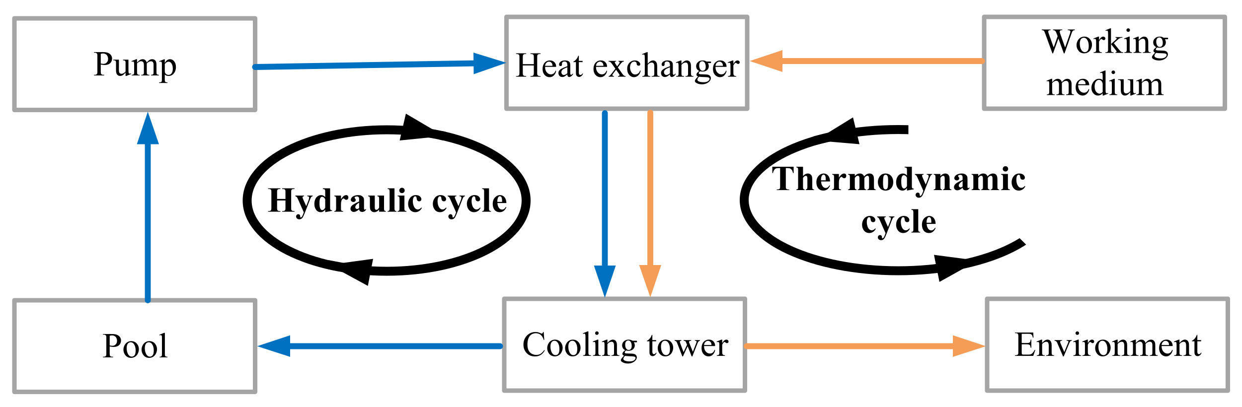
CCWS is a typical heat and mass transfer system with water as a cooling medium (the water is recycled). It is mainly composed of a heat exchanger, cooling tower, water pump, and pipeline. The system operation comprises hydraulic and thermal cycles. The hydraulic cycle can be regarded as a closed cycle, and the thermal cycle is a semi-open cycle, as shown in Figure 1.
The pool is usually regarded as the starting point of a cycle. The cooling water is pressurized by the water pump to a certain pressure energy and transmitted to the heat exchanger network. Then, the flow of each branch is redistributed by adjusting the valve opening. In the heat exchanger, the heat is transferred from the high-temperature working medium side to the cooling water through the tube wall. The heat transfer is affected by the flow mode of cold and hot fluids and the temperature entering the heat exchanger. After heat absorption, the cooling water enters the cooling tower under the action of the residual pressure of the return water of the system to exchange heat with the air again. The cooling water flows evenly from top to bottom after passing through the filler. The air is sucked into the cooling tower by the fan and flows out from bottom to top. The cooling water can be fully in contact with the air and cooled by contact heat transfer and surface evaporation heat transfer. After cooling by the cooling tower, the temperature of the cooling water is restored to the initial state, and the cooling water is stored in the pool for secondary circulation. During this period, the cooling water is lost due to evaporation, entrainment, purged water, leakage, and other reasons. Continuous supply of new water is necessary to keep the liquid level in the pool constant.
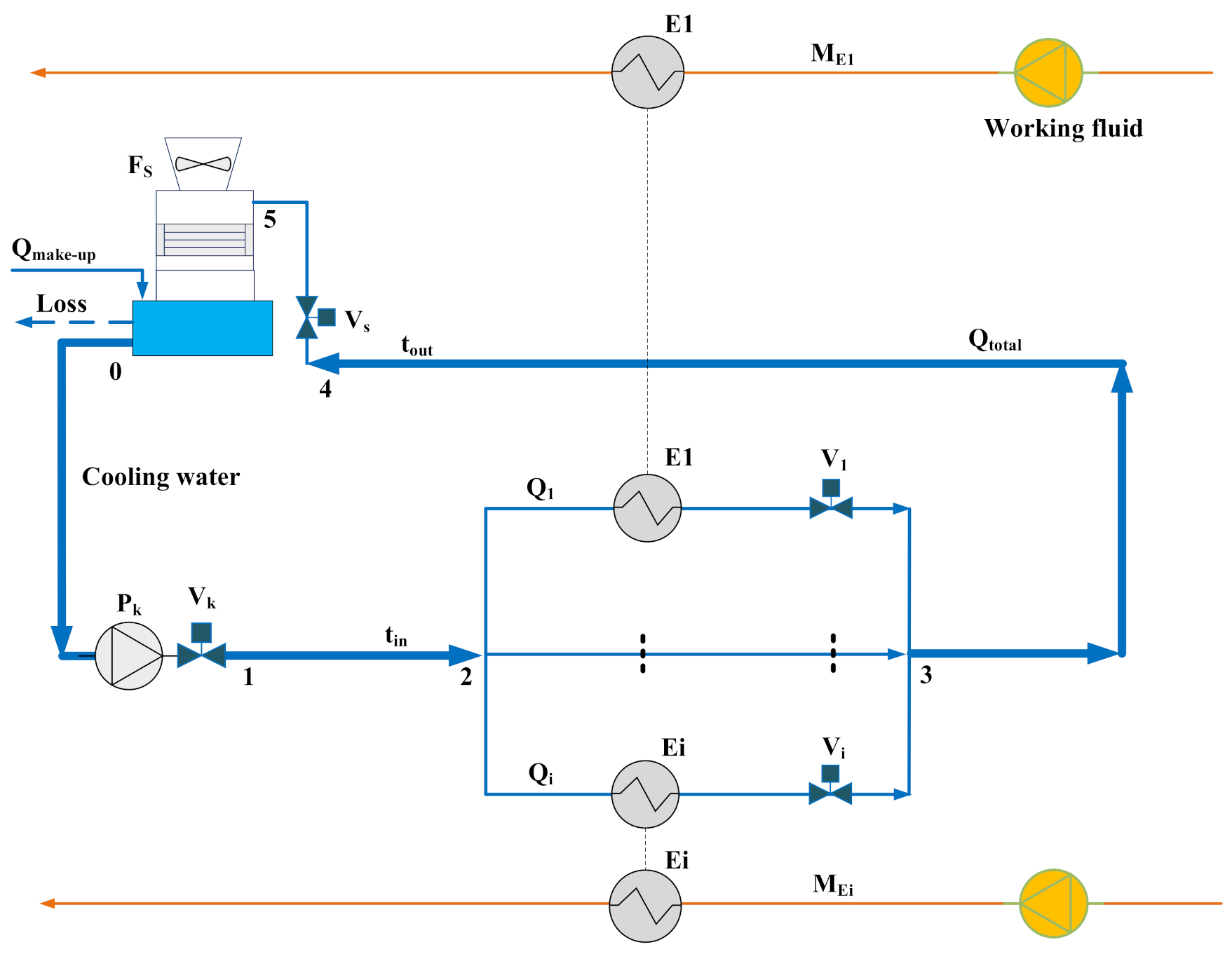
The CCWS superstructure is shown in Figure 2. The cooling water enters the pipe network from position 0 and flows out from position 5. Positions 2 and 3 represent the diversion and confluence points of parallel branches, respectively. In the figure, i is the index of parallel branches, k is the index of parallel pumps, and s is the index of parallel cooling towers. Additionally, is the cooling water supply temperature, is the return temperature of cooling water, represents the working medium flow of heat exchanger Ei, is the cooling water flow of branch i, and is the total flow of the cooling water.
3. Numerical Simulation
3.1. Model Formula
The pressure drop in the common pipe section of parallel branches is small. Minimal heat is dissipated through the pipe surface during the transmission of cooling water in the pipe. The temperature of make-up water is close to that of water supply, and the water volume accounts for only 5% of the total water volume of the system. The load rate of the heat exchanger in many production units changes in the same proportion. Accordingly, the optimal operation model proposed in this study is based on the following assumptions, which aim to simplify the model while controlling the error of model calculation and actual operation within an acceptable range.
- (1)
- The pressure drop in the common section of parallel branches is ignored.
- (2)
- The heat loss of the entire system is ignored.
- (3)
- The effect of make-up water on water supply temperature is ignored.
- (4)
- The load rates of all heat exchangers increase or decrease simultaneously at the same proportion.
Hypothesis (1) aims to simplify the superstructure modeling process and ignore the pressure drop in the common pipe section of parallel branches; it is widely used in superstructure modeling of circulating cooling water systems. Hypotheses (2)–(4) aim to ignore or fix secondary factors that affect the system operation cost.
3.1.1. Heat Exchanger Model Formula
The heat balance equation for the hot and cold fluids inside the heat exchanger is established as follows:
We assume that the heat transfer coefficient at each position in the heat exchanger changes slightly. The heat transfer of the heat exchanger can be expressed as
When the cooling water flow or working medium flow through the heat exchanger changes, the total heat transfer coefficient also changes. For the shell and tube side heat exchanger, when the cooling water goes through the tube side, the following relationship is satisfied [28]:
where represents the shell side heat transfer coefficient in the reference state; represents the fouling thermal resistance in the reference state; and represents the tube side heat transfer coefficient in the reference state, which can be obtained from the operating parameters of the heat exchanger [29]. Xis the ratio of the real working medium flow in the heat exchanger to the working medium flow in the reference state. In this study, it is called the load rate. is the ratio of the real cooling water flow in the heat exchanger to the cooling water flow in the reference state.
The branch flow () can be obtained by simultaneously applying Equations (1)–(3).
In accordance with the mass conservation equation, the total flow of cooling water can be expressed as the sum of the flow of each branch as follows:
The return water temperature of CCWS can be expressed as
The fixed variables involved in the heat exchanger model include . The random variable is the load rate .
3.1.2. Cooling Tower and Fan Model Formula
The thermodynamic calculation of the cooling tower uses the enthalpy difference method [30] proposed by Merkel in 1925.
The left side of the formula is called the characteristic number of the cooling tower, and the right side is called the cooling number of the cooling tower. The Chebyshev integral method is used to solve the integral function on the right side of the formula, as recommended by the American Cooling Tower Association. The accuracy of four interpolation points, which are , is sufficient.
where , , , and represent the difference between saturated and corresponding air enthalpies when the air temperature at each interpolation point is equal to the water temperature.
The enthalpy of air in the cooling tower (), the available air wet bulb temperature (τ), and the corresponding saturated air enthalpy () are . In accordance with the heat balance equation, the enthalpy of air out of the cooling tower () can be expressed as
and in the characteristic number of the cooling tower are the test coefficients of the filler. represents the air–water ratio of the cooling tower, and its value is related to air bulk density , fan air volume (G), ambient dry bulb temperature (), ambient wet bulb temperature (τ), and cooling water flow into the tower (Q).
The Antoine equation is used to calculate saturated steam pressure [31], as follows:
The power consumption of the cooling tower fan can be approximately solved with the method proposed in [23,24]. is a constant that can be obtained through regression between the measured fan power and the fan air volume under different working conditions.
The fixed variables involved in the cooling tower model include . The random variables include and τ. and are obtained from the heat exchanger model.
3.1.3. Pipe Network and Pump Model Formula
The water pump transports the cooling water to the heat exchanger through the pipe network, and the water finally flows into the cooling tower. The pump head should meet two conditions.
Condition 1: The pressure of cooling water at position 5 of the pipe network is greater than or equal to zero.
Condition 2: The pressure of cooling water at the highest point of the branch is greater than or equal to zero.
where is the operating head of the water pump, and the parallel water pump has the same head. is the liquid level in the sump. refer to the head loss of cooling water on the pipeline (see Figure 1 for node position). is the head loss of cooling water on the branch, and it can be calculated with the method presented in [13,14].
The pressure drops of all branches in the parallel pipe network are the same, and they are all equal to the largest one.
Pump delivery power () is equal to the sum of the power of all power frequency pumps and speed regulating pumps. Generally, only one water pump has a VFD.
where con represents the power frequency pump, and var represents the variable frequency pump. The pump head () is determined. and can be obtained in accordance with the performance curve of the water pump. The flow of the variable frequency pump is calculated as
In accordance with the actual operating point (, ) of the variable frequency pump, a parabola () can be obtained, and it is called an equal efficiency parabola. The operating efficiency of the variable frequency pump is equal to the efficiency value at the intersection of the parabola and the performance curve of the rated speed water pump. However, when the pump speed deviates considerably from the rated speed, the relative loss in the pump increases due to the excessive decrease in flow rate in the pump, and the actual isoefficiency curve does not coincide with the parabola. When the rotational speed decreases, the water pump efficiency can be corrected in accordance with the method in [32].
The fixed variables in the pipe network model include , , specifications of the water pump and pipe network, and structural parameters of the heat exchanger. The flow of each pipe section () and the main pipeline flow () are obtained from the heat exchanger model.
3.2. Objective Function
The objective function is the total system operation cost per unit time at the minimum. The total system operation cost includes pump operation cost (), fan operation cost (), and make-up water cost (). The proportion of other costs is extremely small, and the fluctuation is small; thus, these are not considered [20,26].
where is the electricity price, and is the water price. Instantaneous make-up water flow () is equal to all the cooling water lost by the system during this period,
The cooling water loss caused by leakage in the pipe network is an uncertain factor and will not be considered temporarily. According to [33], the amount of water replenishment can be expressed as
where ∂ is the correction coefficient of make-up water, which is obtained through reverse calculation in accordance with the actual operation data.
3.3. Numerical Method
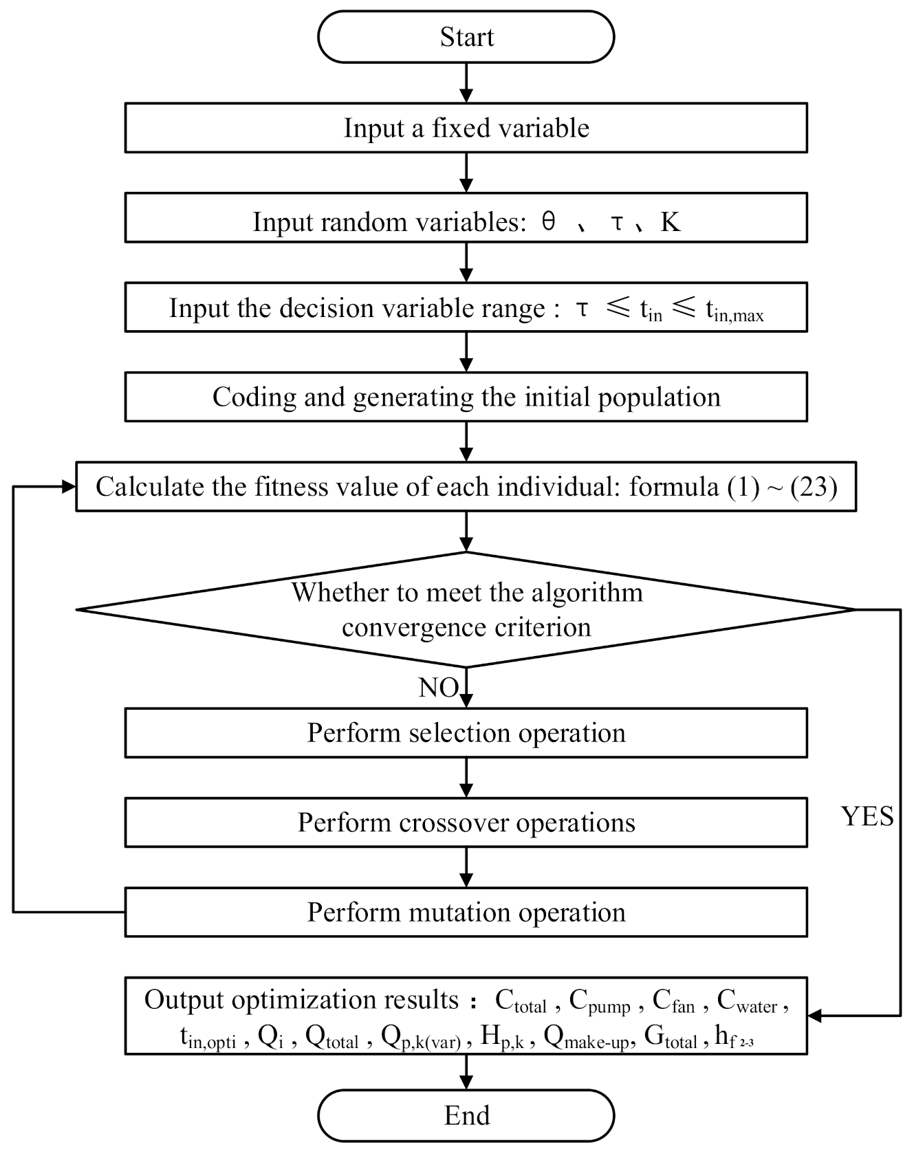
The proposed CCWS operation cost analysis and optimization model is a synchronous optimization of the network structure, equipment operation mode, and equipment operation state, which is a nonlinear programming problem. Therefore, the genetic algorithm toolkit of MATLAB [34] is used to solve this problem, and the flowchart of the numerical simulation is shown in Figure 3. The fixed variables include specifications of the water pump, pipe network, and structural parameters of the heat exchanger. The random variables include , , and X. The cooling water supply temperature () can be connected in series with the operation plan of each module of the system, hence, it is used as a decision variable.
4. Sensitivity of Operation Cost to Ambient Temperature and Working Medium Flow
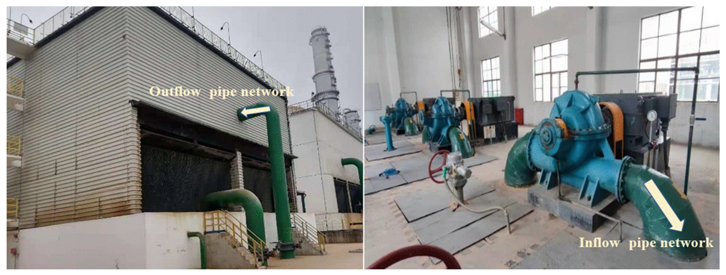
The developed program is an effective tool to study the impact of environmental temperature and load rate changes on the system operation cost. The data used in this section are from the numerical simulation results. The values of ambient dry bulb temperature, ambient wet bulb temperature, and load rate refer to the ambient temperature and production status of the research object.
The research object is a CCWS in Southern China, as shown in Figure 4. The system is equipped with three mechanical ventilation countercurrent cooling towers, five water pumps, and five heat exchangers. The equipment specifications are shown in Table 1. Each cooling tower fan in the system contains a VFD, and the operation of the fan is adjusted in accordance with the water pool temperature. One of the water pumps is also equipped with a VFD. The system controls the supply pressure and flow of cooling water by initializing and stopping the pump and variable frequency pump. The electricity price of the plant is 0.09 $/kWh, and the water price is 0.17 $/m3. The motor efficiency is 95%, and the air pressure is the local atmospheric pressure of 104 kPa (although the atmospheric pressure changes in the entire process, the change is extremely small, and the atmospheric pressure can be regarded as a constant).
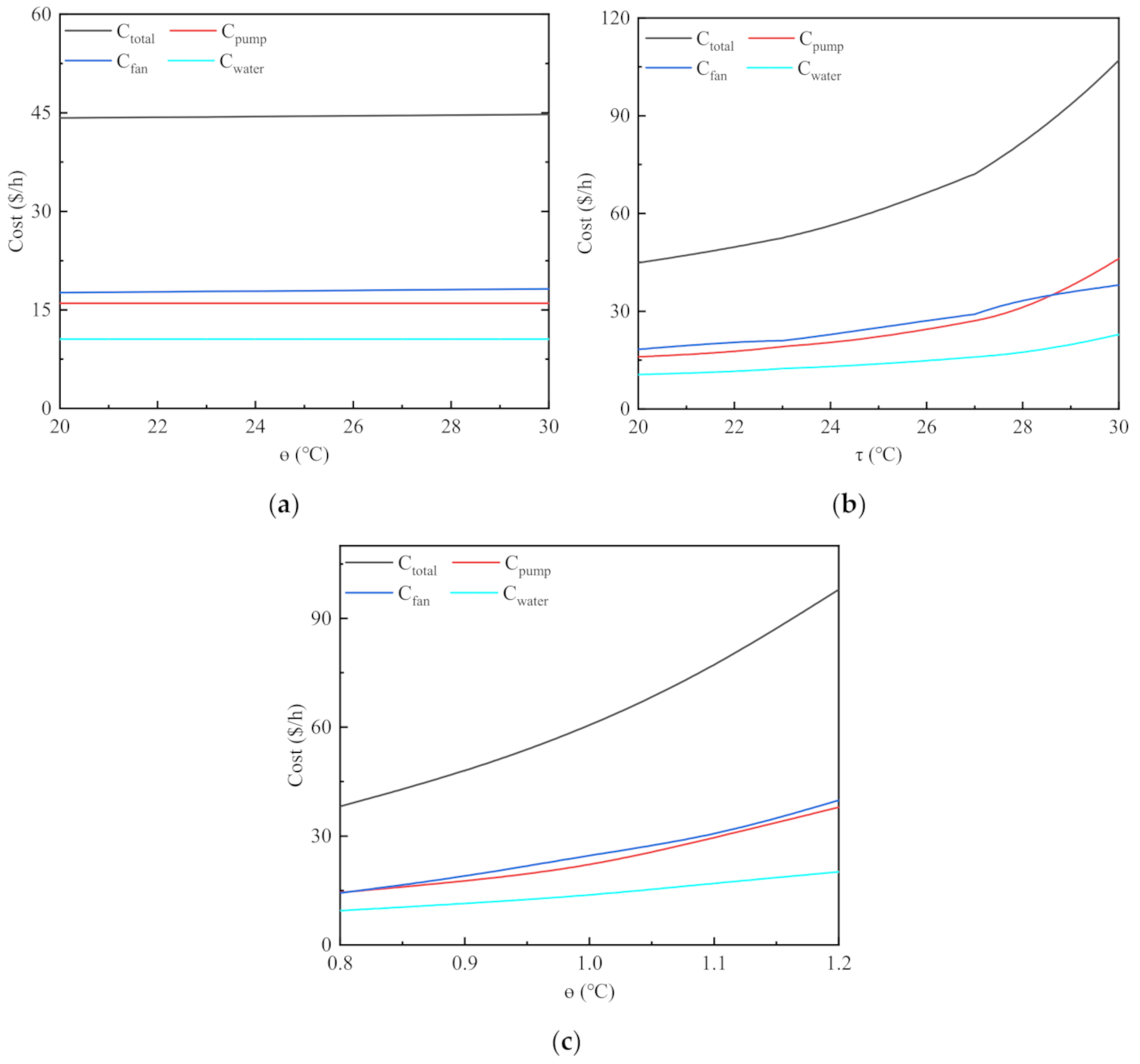
During the sensitivity analysis of ambient dry bulb temperature, its value changes between 20 °C and 30 °C. At this time, the ambient wet bulb temperature and load rate are 20 °C and 100%, respectively. The impact of ambient dry bulb temperature on the operation cost is shown in Figure 5a. The water replenishment cost accounts for the smallest proportion in the total cost, contributing approximately 20–25% to the total cost. The operating cost of the fan is close to that of the water pump, but the operating cost of the water pump is slightly higher than that of the fan. When the ambient dry bulb temperature gradually increases from 20 °C to 30 °C, the operation cost of the fan increases slightly, whereas the operation cost of the water pump and the water replenishment cost do not change. That is, the change in ambient dry bulb temperature does not affect the best operation of the system.
During the sensitivity analysis of the environmental wet bulb temperature, its value changes between 20 °C and 30 °C. At this time, the environmental dry bulb temperature and load rate are 30 °C and 100%, respectively. The impact of ambient wet bulb temperature on the operation cost is shown in Figure 5b. The ambient wet bulb temperature ranges from 20 °C to 30 °C. The operation costs of the system fan, water pump, and make-up water are significantly increased, and the change in the total system operation cost relative to ambient wet bulb temperature is significant. The reason is that the cooling water in the cooling tower is mainly dissipated by evaporation, and the power of evaporation and heat dissipation is the pressure difference between the saturated steam pressure of water and the water vapor in the air. The main factor that influences evaporative heat dissipation is ambient wet bulb temperature rather than ambient dry bulb temperature. Wet bulb temperature is the temperature limit at which the cooling tower can cool the cooling water. Given that the mass transfer and heat exchange efficiency at high wet bulb temperatures are higher than those at low wet bulb temperatures, the increase rate of fan operation cost decreases when the wet bulb temperature is high, as shown in Figure 5b. When the wet bulb temperature is less than 28 °C, the increase rate of fan operation cost increases with the increase in wet bulb temperature. When the wet bulb temperature is greater than 28 °C, the increase rate of fan operation cost suddenly decreases.
In the load rate sensitivity analysis, the value changes between 80% and 120%. At this time, the ambient dry and wet bulb temperatures are 25 °C and 27 °C, respectively. As shown in Figure 5c, with the increase in load rate, the operation cost of the system water pump, make-up water cost, and fan operation cost increase, and the sensitivity of water pump and fan operation costs to load rate are basically the same. The increase in load rate indicates that the heat transferred by the system increases. More cooling water or lower water supply temperature is required in the heat exchange process in the heat exchanger to enhance heat transfer, and more air volume is needed in the heat exchange process in the cooling tower to improve the gas–water ratio.
5. Operation Optimization
Another objective of this work is to provide a method to guide the optimal operation of the system on-site, without resorting to time-consuming simulation when the working conditions change.
5.1. Optimal Water Supply Temperature
According to Equations (2) and (3), reducing the water supply temperature and increasing the cooling water flow can increase the heat transfer of the heat exchanger. The increase in cooling water flow can improve the heat transfer coefficient of the heat exchanger. However, when the cooling water flow is greater than the design value, the increase in the heat transfer coefficient becomes small. At this time, the heat transfer coefficient of the heat exchanger depends on the heat transfer coefficient on the working medium side and the fouling thermal resistance. Furthermore, reducing the water supply temperature can increase the logarithmic average temperature difference of the heat exchanger, which is another way to improve the heat exchange. When the cooling water temperature is similar to the inlet temperature of the working medium, the heat exchange is 0. Conversely, to eliminate the same heat, an increase in water supply temperature requires more cooling water. An increase in water supply temperature is bound to cause an increased pump operation cost. The water supply temperature of the system is considerably important for its operation cost. According to the analysis of the sensitivity of operation cost to ambient temperature and working medium flow, we only need to analyze the variation law of various operating costs with water supply temperature under different ambient wet bulb temperatures and production loads; we do not need to consider the ambient dry bulb temperature.
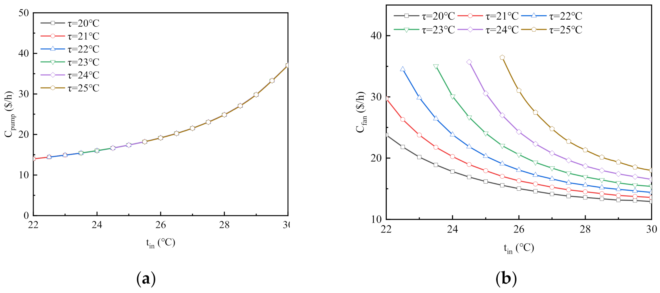
Figure 6 shows the variation law of operation cost relative to water supply temperature under different wet bulb temperatures when the load rate is 100%. As shown in Figure 6a, the operating cost of the water pump increases gradually with the increase in water supply temperature, and the different wet bulb temperatures do not cause a change in the operating cost of the water pump. Figure 6b indicates that with the increase in water supply temperature, the fan operation cost gradually decreases; when the wet bulb temperature is high or the water supply temperature is low, the fan operation cost has a large reduction range. As shown in Figure 6c, the replenishment cost increases gradually with the increase in water supply temperature, and the difference in wet bulb temperature does not cause a change in the replenishment cost, which is similar to the law of pump operation cost. Figure 6d indicates that with the increase in water supply temperature, the total operation cost of the system initially decreases and then increases. An excessively high or excessively low water supply temperature results in a significant increase in operation cost. The higher the wet bulb temperature is, the more sensitive the total operation cost of the system is to the water supply temperature.
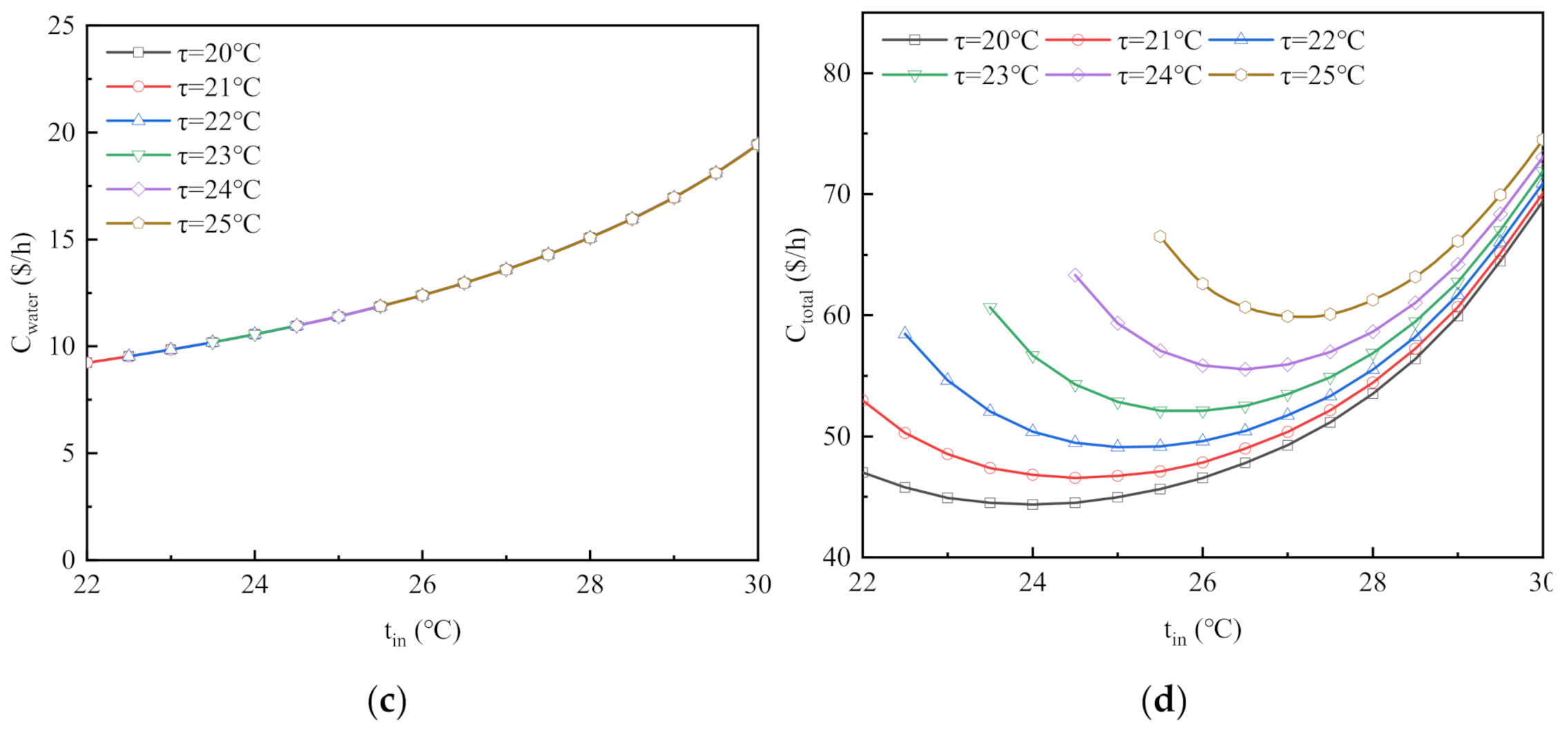
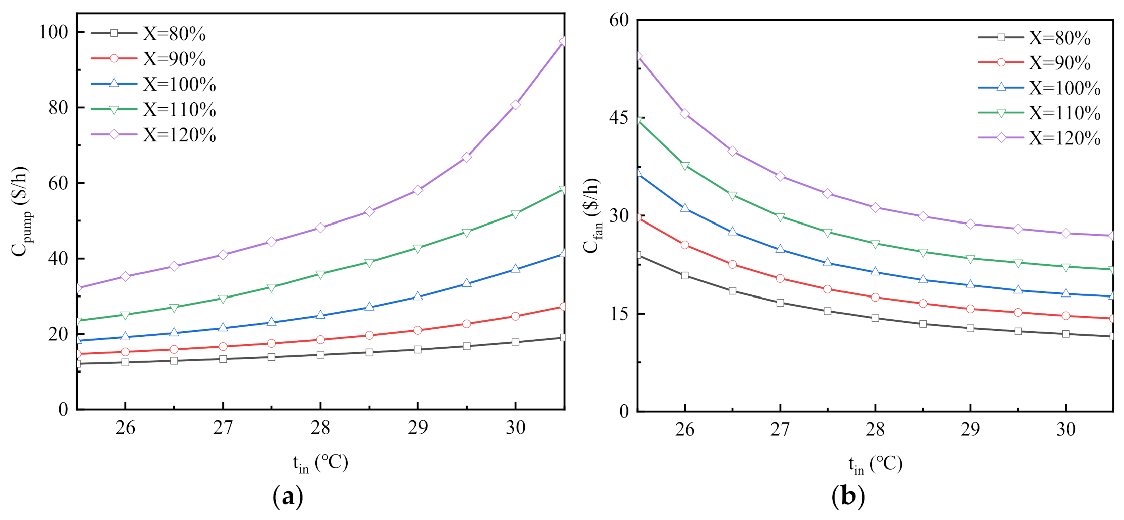
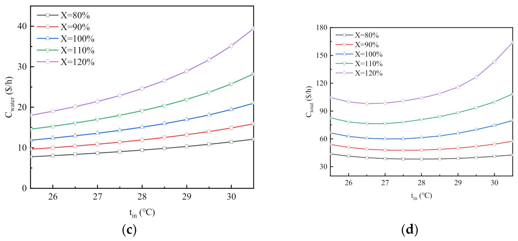
Figure 7 demonstrates the variation law of each operation cost relative to water supply temperature under different load rates when the ambient wet bulb temperature is 25 °C. Figure 7a shows that with the increase in water supply temperature, the operating cost of the water pump gradually increases; the higher the load rate or the higher the water supply temperature, the greater the increment rate of the operating cost of the water pump. As presented in Figure 7b, with the increase in water supply temperature, the fan operation cost gradually decreases; when the load rate is high or the water supply temperature is low, the fan operation cost has a large reduction range. Figure 7c illustrates that with the increase in water supply temperature, the water replenishment cost gradually increases; the higher the load rate or the higher the water supply temperature, the greater the water replenishment cost; this trend is similar to the law of pump operation cost. As shown in Figure 7d, with the increase in water supply temperature, the total operation cost of the system initially decreases and then increases. An extremely low or extremely high water supply temperature causes a significant increase in operation cost. In addition, the higher the load rate, the more sensitive the total operation cost of the system is to the water supply temperature.
The minimum total operation cost of the system (the minimum value of each curve in Figure 6 and Figure 7d can be obtained through the proposed operation optimization model). At this time, the water supply temperature is called the optimal water supply temperature. The optimal water supply temperature under different ambient temperatures and load rates is the focus of engineers and the problem to be solved in this section.
5.2. Correlation of Optimal Water Supply Temperature with Ambient Wet Bulb Temperature and Load Rate
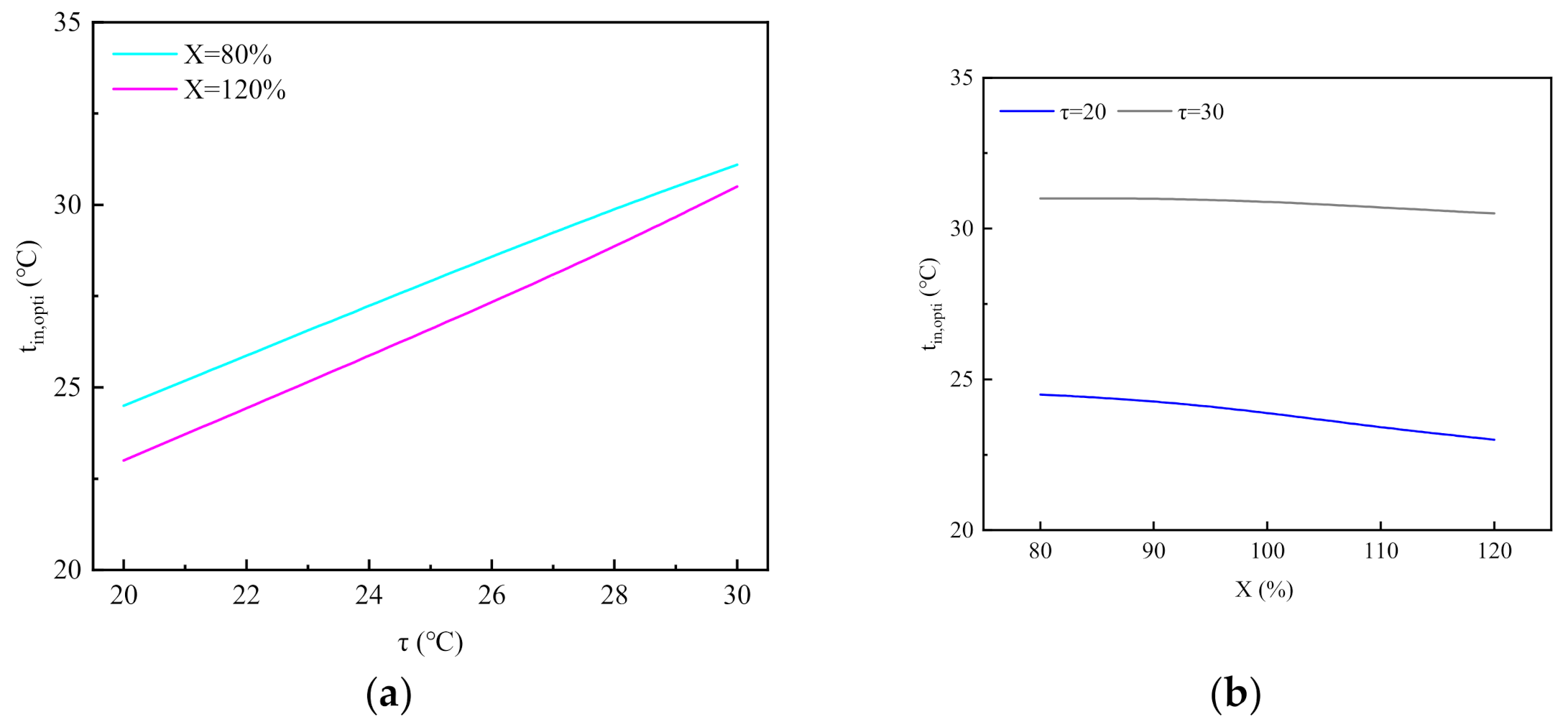
Figure 8a shows the correlation between the optimal water supply temperature of the system and ambient wet bulb temperature. With the increase in ambient wet bulb temperature, the optimal water supply temperature increases considerably, and the high load rate strengthens the effect of ambient wet bulb temperature on the optimal water supply temperature. Figure 8b presents the relationship between the optimal water supply temperature and the load rate of the system. The optimal water supply temperature decreases slightly with the increase in load rate, and the effect becomes small when the ambient wet bulb temperature is high. According to the change rate of the optimal water supply temperature with ambient wet bulb temperature and load rate, the effect of wet bulb temperature on water supply temperature is much higher than the effect of load rate.
Several calculation results for the case model are listed in Table 2.
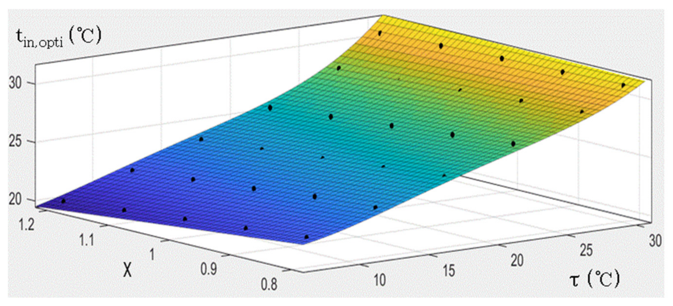
The polynomials associated with the data in Table 2 are obtained through the subroutine cftool function in MATLAB software, and the optimal values of each coefficient are shown in Table 3.
The goodness of fit is shown in Figure 9, and the optimal values of each coefficient are shown in Table 3. When the ambient wet bulb temperature is 15–30 °C and the load rate is 80–120%, Equation (24) can simply and rapidly calculate the optimal water supply temperature of the system on the premise of ensuring accuracy.
5.3. Method Validation
Equation (24) can guide engineers in the optimization of the water supply temperature of the system under changing wet bulb temperatures or load rates and the total operation cost of the system. We perform optimal scheduling experiments on the research system with the help of engineers to verify the reliability of the proposed method. The calculated and actual values of the total operation cost under seven experimental conditions and their error rates are listed in Table 4. Errors occur because the model ignores secondary influencing factors, and partly because of the measurement and data statistics errors of the field instruments. As shown in Table 4, the calculated total operation cost is very close to the actual total operation cost and the error range under seven groups of experimental conditions is basically within 5%. Hence, the proposed method is reliable.
5.4. Optimization Effect
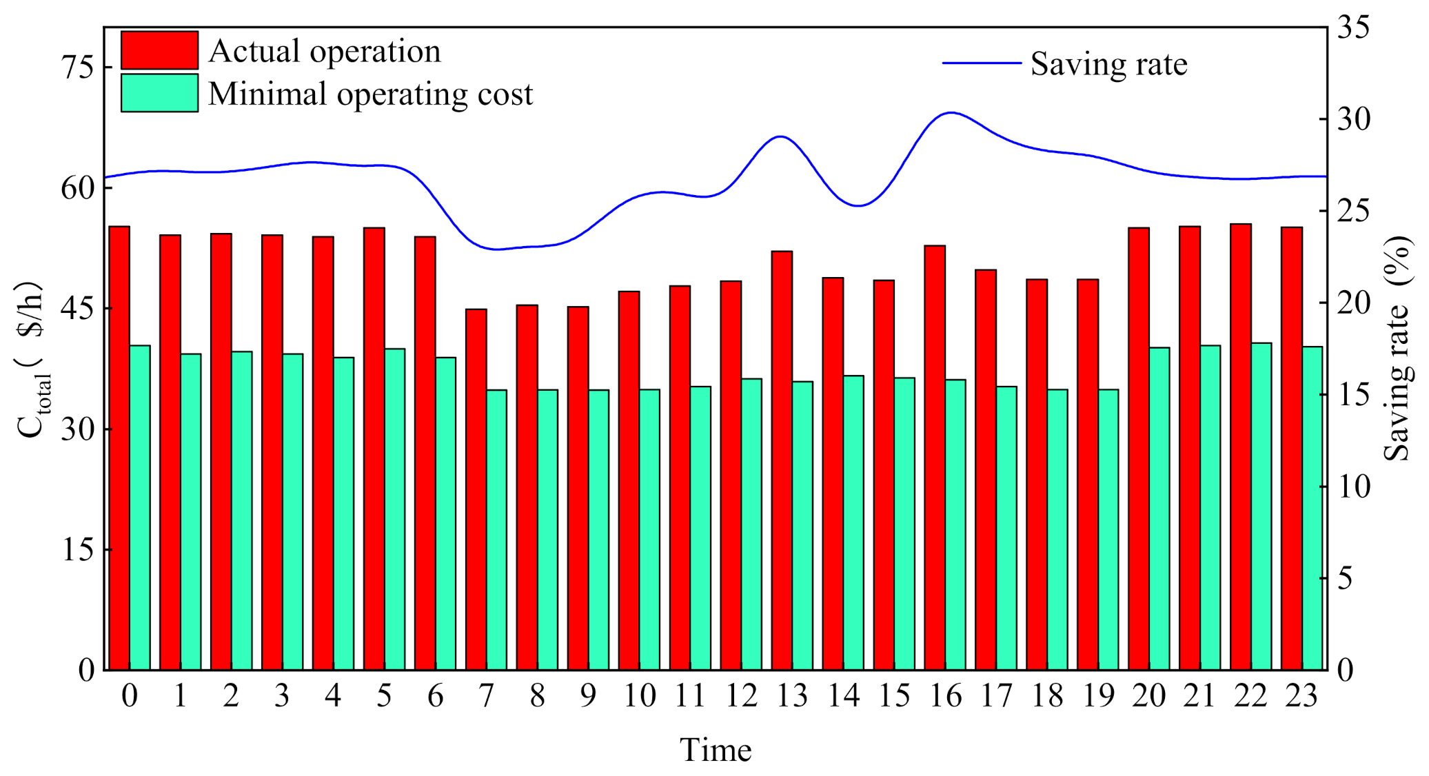
To verify the real effect of the proposed operation optimization method, the operation cost controlled by the optimal water supply temperature control equation is compared with the actual operation cost. Table 5 shows the actual 24-h operation data of the system on a certain day in April, and it includes the required ambient wet bulb temperature, load rate, and actual water supply temperature. With the ambient wet bulb temperature and system load rate at different times in Table 5, the optimal water supply temperature can easily be obtained through Equation (24). Then, the pressure and flow of the system can be adjusted to approach the minimum operation cost.
Figure 10 shows a comparison of the actual and optimized operation costs. In one day of sampling, the cost saving rate is as low as 22% and as high as 31%. The comparison results show that this method can effectively reduce the operation cost of the system and increase the profit of the enterprise.
6. Conclusions
An operation cost analysis and optimization model based on the superstructure method is proposed through an in-depth analysis of CCWS. The model considers the effect of the installation height of the heat exchanger when calculating the operation cost of the water pump (Equation (15)). The model uses ambient dry bulb temperature, ambient wet bulb temperature, and load rate as random variables. Other process parameters are employed as fixed variables to quantify the impact of weather conditions and working medium flow on the system operation cost. In addition, operation optimization based on the minimum cost is performed, and the relationship among ambient wet bulb temperature, load rate, and optimal water supply temperature of the system is analyzed to determine the optimal water supply temperature in consideration of the changes in climate and working medium flow. The main conclusions are as follows:
- (1)
- The effect of ambient dry bulb temperature on the total system operation cost is extremely small and can be ignored. The operating costs of the cooling tower fan, water pump, and make-up pump are highly sensitive to ambient wet bulb temperature and working medium flow. They increase rapidly with the increase in ambient wet bulb temperature or load rate.
- (2)
- With the increase in water supply temperature, the total operation cost of the system initially decreases then increases. An extremely low or extremely high water supply temperature causes a significant increase in operation cost. With the increase in wet bulb temperature or load rate, the total operation cost of the system becomes increasingly sensitive to water supply temperature.
- (3)
- The optimal water supply temperature and ambient wet bulb temperature increase and decrease at the same time, and a high load rate strengthens the effect of ambient wet bulb temperature on the optimal water supply temperature. The optimal water supply temperature decreases slightly with the increase in load rate, and a high ambient wet bulb temperature weakens the effect of load rate on the optimal water supply temperature.
- (4)
- The optimization results show that considering the changes in ambient wet bulb temperature and working medium flow can effectively reduce the operation cost of the system. The control equation for the optimal water supply temperature can guide the system to adapt to the current working conditions for operation optimization and can facilitate the planning of future working conditions. It can also help evaluate the capability of the system to deal with extreme wet bulb temperature or extreme load rate. A control equation for optimal water supply temperature that is similar to Equation (24) should be customized for all systems.
Author Contributions
Investigation, optimization model establishment, data analysis, and paper writing were carried out by P.W., X.L. and S.C. conceived and supervised the study and edited the manuscript; and Q.C. and J.L. completed the programming. All authors have read and agreed to the published version of the manuscript.
Funding
This study was supported by the National Natural Science Foundation of China (Grant nos. 51879216 and 51527808).
Conflicts of Interest
The authors declare no conflict of interest.
Nomenclature
The following abbreviations are used in this manuscript:
| CCWS | Circulating cooling water system |
| VFD | Variable frequency drive |
| List of Symbols | |
| Heat transfer area | |
| Test factor of filler | |
| Specific heat of the working medium | |
| Specific heat of cooling water | |
| Fan operational cost | |
| Pump operational cost | |
| Total operating cost | |
| Cost of make-up water | |
| d | Tube inner diameter |
| Air enthalpy | |
| Enthalpy of saturated air | |
| Acceleration of gravity | |
| Total air flow | |
| Height of the heat exchanger | |
| Liquid level height | |
| Head loss from node 0 to node 2 (Figure 1) | |
| Head loss on branch i | |
| Operating head of the pump | |
| Heat coefficient taken away by evaporated water | |
| Convective heat transfer coefficient of the shell side in reference state | |
| Convective heat transfer coefficient of the tube side in reference state | |
| L | Tube length |
| Working medium flow | |
| Flow of working medium in reference state | |
| Number of tubes in a heat exchanger | |
| Number of concentration cycles | |
| Number of tube passes of a heat exchanger | |
| Atmospheric pressure | |
| Instantaneous power of the pump | |
| Instantaneous power of the fan | |
| Electricity price | |
| Water price | |
| Saturated water vapor pressure | |
| Water flowrate lost by entrainment | |
| Water flowrate lost by evaporation | |
| Flow of cooling water in reference state | |
| Flow of cooling water on branch i | |
| Water flowrate lost by leakage | |
| Make-up water flow | |
| Purged water flowrate | |
| Total flow of cooling water | |
| Dirt thermal resistance | |
| Cooling water outlet temperature | |
| System supply water temperature | |
| Optimal water supply temperature | |
| System return water temperature | |
| Working medium inlet temperature | |
| Working medium outlet temperature | |
| Production load rate | |
| Cooling water flow ratio | |
| Heat exchange | |
| Relative humidity | |
| Correction coefficient of make-up water flow | |
| Test factor of filler | |
| Air–water ratio | |
| Environmental dry bulb temperature | |
| Environmental wet bulb temperature | |
| Density of cooling water | |
| Density of air | |
| Pump operation efficiency | |
| Pump motor operating efficiency | |
| Constants related to a fan | |
| Large temperature difference between both sides | |
| Small temperature difference between both sides | |
| Pressure loss of a heat exchanger | |
| Pressure loss of a branch pipeline |
References
- Huang, M.-T.; Zhai, P.-M. Achieving Paris Agreement temperature goals requires carbon neutrality by middle century with far-reaching transitions in the whole society. Adv. Clim. Chang. Res. 2021, 12, 281–286. [Google Scholar] [CrossRef]
- Zhu, X.; Wang, F.; Niu, D. Energy-saving transformation of circulating cooling water system based on energy-saving bottleneck diagnosis. Control Decis. China 2019, 35, 8. [Google Scholar]
- Suo, R.; Wang, Y.; Feng, X. Optimization of circulating water network considering heat transfer enhancement. Comput. Appl. Chem. 2015, 32, 1439–1442. [Google Scholar]
- Chen, L. Energy Saving and Emission Reduction Technology in Industrial Circulating Water System; Anhui Jianzhu University: Hefei, China, 2017. [Google Scholar]
- Linnhoff, B.; Hindmarsh, E. The pinch design method for heat exchanger networks. Chem. Eng. Sci. 1983, 38, 745–763. [Google Scholar] [CrossRef]
- Polley, G.T.; Shahi, M.H. Interfacing Heat Exchanger Network Synthesis and Detailed Heat Exchanger Design. Chem. Eng. Res. Des. 1991, 69, 445–457. [Google Scholar]
- Panjeshahi, M.; Tahouni, N. Pressure drop optimisation in debottlenecking of heat exchanger networks. Energy 2008, 33, 942–951. [Google Scholar] [CrossRef]
- Jiang, N.; Lin, L.; Wang, L. Heat exchanger network integration considering pressure drops and multiple shells. CIESC J. 2013, 64, 4128–4136. [Google Scholar]
- Torkfar, F.; Avami, A. A simultaneous methodology for the optimal design of integrated water and energy networks considering pressure drops in process industries. Process. Saf. Environ. Prot. 2016, 103, 442–454. [Google Scholar]
- Sun, J.; Feng, X.; Wang, Y.; Deng, C.; Chu, K.H. Pump network optimization for a cooling water system. Energy 2014, 67, 506–512. [Google Scholar] [CrossRef]
- Ma, J.; Wang, Y.; Feng, X. Simultaneous optimization of pump and cooler networks in a cooling water system. Appl. Therm. Eng. Des. Process. Equip. Econ. 2017, 125, 377–385. [Google Scholar] [CrossRef]
- Zhang, H.; Feng, X.; Wang, Y.; Zhang, Z. Sequential optimization of cooler and pump networks with different types of cooling. Energy 2019, 179, 815–822. [Google Scholar] [CrossRef]
- Ma, J.; Wang, Y.; Feng, X. Energy recovery in cooling water system by hydro turbines. Energy 2017, 139, 329–340. [Google Scholar] [CrossRef]
- Gao, W.; Feng, X. The power target of a fluid machinery network in a circulating water system. Appl. Energy 2017, 205, 847–854. [Google Scholar] [CrossRef]
- Gao, W.; Feng, X. Synthesis of the fluid machinery network in a circulating water system. Chin. J. Chem. Eng. 2019, 27, 114–124. [Google Scholar] [CrossRef]
- Lee, H.; Teo, K.; Cai, X. An optimal control approach to nonlinear mixed integer programming problems. Comput. Math. Appl. 1998, 36, 87–105. [Google Scholar] [CrossRef] [Green Version]
- Kim, J.-K.; Smith, R. Automated retrofit design of cooling-water systems. AIChE J. 2003, 49, 1712–1730. [Google Scholar] [CrossRef]
- Panjeshahi, M.H.; Ataei, A. Application of an environmentally optimum cooling water system design in water and energy conservation. Int. J. Environ. Sci. Technol. 2008, 5, 251–262. [Google Scholar]
- Ma, J. Simultaneous Optimization of Cooler Network, Pump Network, and Cooling Tower. In Proceedings of the 27th European Symposium on Computer Aided Process Engineering, Part A, Barcelona, Spain, 1–5 October 2017; pp. 763–768. [Google Scholar]
- Zhu, X.; Wang, F.; Niu, D.; Zhao, L. Integrated Modeling and Operation Optimization of Circulating Cooling Water System Based on Superstructure. Appl. Therm. Eng. 2017, 127, 1382–1390. [Google Scholar] [CrossRef]
- Zhao, S. The Principle of Cooling Tower Technology; China Construction Industry Press: Beijing, China, 2015. [Google Scholar]
- Muangnoi, T.; Asvapoositkul, W.; Wongwises, S. Effects of inlet relative humidity and inlet temperature on the performance of counterflow wet cooling tower based on exergy analysis. Energy Convers. Manag. 2008, 49, 2795–2800. [Google Scholar] [CrossRef]
- Hajidavalloo, E.; Shakeri, R.; Mehrabian, M.A. Thermal performance of cross flow cooling towers in variable wet bulb temperature. Energy Convers. Manag. 2010, 51, 1298–1303. [Google Scholar] [CrossRef]
- Papaefthimiou, V.; Rogdakis, E.; Koronaki, I.; Zannis, T. Thermodynamic study of the effects of ambient air conditions on the thermal performance characteristics of a closed wet cooling tower. Appl. Therm. Eng. 2012, 33–34, 199–207. [Google Scholar] [CrossRef]
- Pontes, R.F.; Yamauchi, W.M.; Silva, E.K. Analysis of the Effect of Seasonal Climate Changes on Cooling Tower Efficiency, and Strategies for Reducing Cooling Tower Power Consumption. Appl. Therm. Eng. 2019, 161, 114148. [Google Scholar] [CrossRef]
- Castro, M.M.; Song, T.W.; Pinto, J.M. Minimization of Operational Costs in Cooling Water Systems. Chem. Eng. Res. Des. 2000, 78, 192–201. [Google Scholar] [CrossRef]
- Liao, J.; Xie, X.; Nemer, H.; Claridge, D.E.; Culp, C.H. A simplified methodology to optimize the cooling tower approach temperature control schedule in a cooling system. Energy Convers. Manag. 2019, 199, 111950.1–111950.9. [Google Scholar] [CrossRef]
- Liu, W. Handbook of Process Calculation for Cold Exchange Equipment; China Petrochemical Press: Beijing, China, 2003. [Google Scholar]
- Yu, J.Z. Principle and Design of Heat Exchanger; Beijing University of Aeronautics and Astronautics Press: Beijing, China, 2006. [Google Scholar]
- Merkel, F. Verdunstungskühlung; No. 275, Verdunstungskuhlung; VDI Forschungsarbeiten: Berlin, Germany, 1925. [Google Scholar]
- Chen, X.Z.; Cai, Z.Y.; Hu, W.M. Chemical Engineering Thermodynamics, 2nd ed.; Chemical Industry Press: Beijing, China, 2008. [Google Scholar]
- Guan, X.F. Modern Pump Theory and Design; China Aerospace Press: Beijing, China, 2011. [Google Scholar]
- Perry, R.H.; Green, D. Perry’s Chemical Engineers’ Handbook; McGraw Hill: New York, NY, USA, 1997. [Google Scholar]
- The Mathworks Matlabs Optimization Toolbox. USA. 2017. Available online: https://www.mathworks.com/ (accessed on 25 August 2021).
Figure 1.
Schematic of hydraulic and thermal cycles in CCWS.

Figure 2.
Superstructure of CCWS.

Figure 3.
Sensitivity of operation cost to ambient temperature and working medium flow.

Figure 4.
Cooling tower and water pump of the research object.

Figure 5.
Variation in operating cost relative to ambient dry bulb temperature, ambient wet bulb temperature, and load rate. (a) Ambient dry bulb temperature. (b) Ambient wet bulb temperature. (c) Load rate.
Figure 5.
Variation in operating cost relative to ambient dry bulb temperature, ambient wet bulb temperature, and load rate. (a) Ambient dry bulb temperature. (b) Ambient wet bulb temperature. (c) Load rate.

Figure 6.
Variation law of operation cost relative to water supply temperature under different wet bulb temperatures. (a) Pump operation cost. (b) Fan operation cost. (c) Make-up water cost. (d) Total operating cost.
Figure 6.
Variation law of operation cost relative to water supply temperature under different wet bulb temperatures. (a) Pump operation cost. (b) Fan operation cost. (c) Make-up water cost. (d) Total operating cost.


Figure 7.
Variation law of operation cost relative to water supply temperature under different load rates. (a) Pump operation cost. (b) Fan operation cost. (c) Make-up water cost. (d) Total operating cost.
Figure 7.
Variation law of operation cost relative to water supply temperature under different load rates. (a) Pump operation cost. (b) Fan operation cost. (c) Make-up water cost. (d) Total operating cost.


Figure 8.
Correlation of optimal water supply temperature with ambient wet bulb temperature and load rate. (a) Ambient wet bulb temperature. (b) Load rate.
Figure 8.
Correlation of optimal water supply temperature with ambient wet bulb temperature and load rate. (a) Ambient wet bulb temperature. (b) Load rate.

Figure 9.
Goodness of fit results.

Figure 10.
Comparison of operation cost before and after optimization.


Table 1.
Equipment specification data.
| Unit | Performance Parameter | ||||||
|---|---|---|---|---|---|---|---|
| Pump | |||||||
| (= 43.84, = 8.70.10−3, = 3.33.10−6, = 0.34, = 4.22.10−4, = 7.77.10−8) | |||||||
| Heat Exchanger | Ei | d (m) | L (m) | n | Np | A (m2) | (m) |
| E1 | 0.019 | 12.9 | 1930 | 1 | 1602 | 26 | |
| E2 | 0.019 | 12.6 | 1750 | 1 | 1413 | 11 | |
| E3 | 0.019 | 11.0 | 1391 | 1 | 980 | 9 | |
| E4 | 0.019 | 10.8 | 923 | 1 | 639 | 9 | |
| E5 | 0.020 | 6.0 | 872 | 1 | 399 | 5 | |
| Cooling Tower | , , | ||||||
Table 2.
Optimum water supply temperature under different ambient wet bulb temperatures and load rates.
Table 2.
Optimum water supply temperature under different ambient wet bulb temperatures and load rates.
| = 110% | = 120% | ||||
|---|---|---|---|---|---|
| τ = 15 °C | 22 | 21.5 | 21 | 20.5 | 20 |
| τ = 18 °C | 23.7 | 23.4 | 22.8 | 22.3 | 21.8 |
| τ = 21 °C | 25.5 | 25 | 24.5 | 24 | 23.6 |
| τ = 24 °C | 27.5 | 27 | 26.5 | 26 | 25.5 |
| τ = 27 °C | 29.3 | 29 | 28.6 | 28.2 | 28 |
| τ = 30 °C | 31.1 | 31 | 30.9 | 30.7 | 30.5 |
Table 3.
Best coefficients of polynomials obtained.
| Coefficient | Optimal Value | Unit |
|---|---|---|
| 28.79 | °C | |
| −1.08 | [-] | |
| −8.131 | °C | |
| 0.1266 | °C−1 | |
| 0.7711 | [-] | |
| −0.004387 | °C−2 | |
| −0.05576 | °C−1 | |
| 4.999 × 10⁻⁵ | °C−3 | |
| 0.001247 | °C−2 |
Table 4.
Comparison of calculation results and actual operation.
| Working Conditions | 1 | 2 | 3 | 4 | 5 | 6 | 7 |
|---|---|---|---|---|---|---|---|
| τ (°C) | 16.0 | 21.5 | 23.7 | 18.5 | 26.8 | 25.7 | 20.8 |
| X (%) | 110 | 105 | 100 | 110 | 90 | 95 | 110 |
| Model calculation Ctotal ($/h) | 39.2 | 46.6 | 49.6 | 43.0 | 52.1 | 53.2 | 50.5 |
| Actual operation Ctotal ($/h) | 40.5 | 47.6 | 52.0 | 45.3 | 51.5 | 51.7 | 52.4 |
| Error rate (%) | 3.3 | 2.2 | 4.6 | 5.1 | −1.2 | −2.9 | 3.6 |
Table 5.
Actual operation data of a day.
| Time | 0 | 1 | 2 | 3 | 4 | 5 | 6 | 7 | 8 | 9 | 10 | 11 |
|---|---|---|---|---|---|---|---|---|---|---|---|---|
| τ (°C) | 17.1 | 16.2 | 16.5 | 16.2 | 15.7 | 16.8 | 15.7 | 16.3 | 16.9 | 16.6 | 17 | 18 |
| X (%) | 110 | 110 | 110 | 110 | 110 | 110 | 110 | 100 | 100 | 100 | 100 | 100 |
| tin (°C) | 26 | 26 | 26 | 26 | 26 | 26 | 26 | 26.5 | 26.5 | 26.5 | 27 | 27 |
| Time | 12 | 13 | 14 | 15 | 16 | 17 | 18 | 19 | 20 | 21 | 22 | 23 |
| τ (°C) | 19.1 | 18.8 | 19.4 | 19.2 | 19 | 18 | 17.1 | 17.1 | 16.9 | 17.1 | 17.3 | 17 |
| X (%) | 100 | 100 | 100 | 100 | 100 | 100 | 100 | 100 | 110 | 110 | 110 | 110 |
| tin (°C) | 27 | 28 | 28 | 28 | 28 | 28 | 27.5 | 27.5 | 26 | 26 | 26 | 26 |
Publisher’s Note: MDPI stays neutral with regard to jurisdictional claims in published maps and institutional affiliations. |
© 2021 by the authors. Licensee MDPI, Basel, Switzerland. This article is an open access article distributed under the terms and conditions of the Creative Commons Attribution (CC BY) license (https://creativecommons.org/licenses/by/4.0/).
Share and Cite
MDPI and ACS Style
Wang, P.; Lu, J.; Cai, Q.; Chen, S.; Luo, X. Analysis and Optimization of Cooling Water System Operating Cost under Changes in Ambient Temperature and Working Medium Flow. Energies 2021, 14, 6903. https://doi.org/10.3390/en14216903
AMA Style
Wang P, Lu J, Cai Q, Chen S, Luo X. Analysis and Optimization of Cooling Water System Operating Cost under Changes in Ambient Temperature and Working Medium Flow. Energies. 2021; 14(21):6903. https://doi.org/10.3390/en14216903
Chicago/Turabian StyleWang, Peng, Jinling Lu, Qingsen Cai, Senlin Chen, and Xingqi Luo. 2021. "Analysis and Optimization of Cooling Water System Operating Cost under Changes in Ambient Temperature and Working Medium Flow" Energies 14, no. 21: 6903. https://doi.org/10.3390/en14216903
Note that from the first issue of 2016, this journal uses article numbers instead of page numbers. See further details here.