Insights into Partial Slips and Temperature Jumps of a Nanofluid Flow over a Stretched or Shrinking Surface

Abstract

This paper elucidates the significance of partial slips and temperature jumps on the heat and mass transfer of a boundary layer nanofluid flowing through a stretched or shrinking surface. Considerable consideration is given to the dynamic properties of the nanofluid process, including Brownian motion and thermophoresis. A similarity transform is introduced to obtain a physical model of nonlinear ordinary differential equations, and the Chebyshev method of collocation is used to numerically analyze the influences of parameters of physical flow such as slip, temperature jump, Brownian motion, thermophoresis, suction (or injection) parameters, and Lewis and Prandtl numbers. The numerical results for temperature and concentration profiles, and heat and mass transfer rates, are graphically represented, and insights into the effects of slips and temperature jumps are revealed. In the case of a stretched sheet, the slip parameter enhances the temperature field and increases the thermal boundary layer thickness as well as the concentration function’s boundary layer thickness. When the slip parameter is raised in the case of the shrinking sheet, the dual solutions for temperature and concentration functions are reduced. For the first solution, both the temperature and concentration functions drop as the slip parameter increases, but for the second solution, both the temperature and concentration functions rise as the slip parameter increases. The discoveries have applications in a number of disciplines, including heat transfer in a solar energy collector. Glass blowing, annealing, and copper wire thinning are just a few of the technical and oilfield applications for the current problem. In high-temperature industrial applications, radiation heat transfer research is critical.

1. Introduction

Nanofluid mechanics have become one of the most noteworthy technologies in energy, nanotechnology, tissue engineering, medicine, material science, chemistry, textile engineering, and in the field of renewable energy sources because of their distinctive thermal, electrical, and chemical properties [1,2,3,4,5,6]. The author of ref. [1] investigated seven slip processes that might result in a relative velocity between the nanoparticles and the base fluid. Inertia, Brownian diffusion, thermophoresis, diffusiophoresis, the Magnus effect, fluid drainage, and gravity are examples of these. Only Brownian diffusion and thermophoresis, according to the author, are major slip processes in nanofluids. The findings given in ref. [2] show that nanofluids comprising smaller and better conductivity copper nanoparticles achieve substantially greater increases in effective thermal conductivity. Ref. [3] discusses the synthesis, fluid stabilization, and surface modification of superparamagnetic iron oxide nanoparticles, as well as their applications in biomedical fields such as magnetic resonance imaging contrast enhancement, tissue repair, immunoassay, detoxification of biological fluids, hyperthermia, drug delivery, and cell separation, among others. All of these biomedical and bioengineering applications need high magnetization values and particle sizes of less than 100 nm, with an overall narrow particle size range, to ensure that the particles have homogeneous physical and chemical properties. The important variables in understanding the thermal characteristics of nanofluids, according to Keblinski et al. [4], are the ballistic, rather than diffusive, nature of heat transport in nanoparticles, along with fluid-mediated clustering effects that provide pathways for rapid heat transfer. Furthermore, the boundary conditions, e.g., porous boundaries, deformable boundaries, slips and temperature jumps, will also greatly affect the nanofluid processing [1,2,3,4].

The research of Xiong et al. [5] provides a detailed overview of the usage of hybrid nanofluids in solar collectors. Thermal efficiency was discovered to be proportionately dependent on the fraction of nanoparticles in regular fluids with acceptable values. Aneli et al. [6] investigated the consequences of switching the cooling fluid of a PV/T system from pure water to a nanofluid comprising water and aluminum oxide (Al₂O₃). It was found that increasing the thermal level causes a minor increase in the operating temperatures of the PV, resulting in a tiny drop in the amount of energy produced. Elgazery and Elelamy [7] proposed dual solutions for non-Newtonian Casson nanofluid flow through a moving stretched sheet, with variable thermal conductivity and nonlinear thermal radiation effects, through a porous medium with convective boundary conditions. Their findings are extremely relevant in medicine, particularly in strengthening medication administration through the skin, because drug trapping by nanoparticles improves drug transport to, or absorption by, target cells. It has been widely proven that a small volumetric fraction (less than 5%) of nanoparticles suspended in a base non-Newtonian fluid can increase the thermal conductivity by 10–50% [5,6,7].

Dual solutions for the flow through a nonlinearly decreasing sheet with slip conditions, in the presence of suction, were previously obtained [8]. It was discovered that the momentum boundary layer thickness for the first solution reduces with slip and suction parameters, but rises with the power-law index of the decreasing velocity. The computational examination of steady, magnetohydrodynamic boundary-layer slip flow of a nanofluid across a permeable stretching/shrinking sheet with heat radiation, using RKF45 with a shot approach, was addressed in previous work [9]. According to the findings, the Nusselt number falls with the increasing of the thermophoresis parameter and the thermal slip parameter, but rises with the increasing of the thermal radiation and the Prandtl number. Analysis was provided in ref. [10] to examine the dual nature of mass transfer with first-order chemical reactions in boundary layer stagnation-point flow across a stretching/shrinking sheet. According to the results of this study, dual solutions for the velocity field and the concentration distribution are obtained for particular values of the velocity ratio parameter. The authors of [11] investigated the topic of unsteady magnetohydrodynamic (MHD) stagnation point flow in a viscous fluid across a stretching/shrinking sheet with viscous dissipation and ohmic heating. Dual (first and second) solutions were discovered to exist exclusively for the decreasing sheet situation. It was also discovered that the magnetic and unsteadiness factors have a significant impact on fluid flow and heat transmission. Ref. [12] investigated the numerical simulation of MHD boundary layer flow with heat and mass transport of a nanofluid, with viscous dissipation, across a nonlinear stretching sheet embedded in a porous medium. It was observed that the Brownian motion parameter and the thermophoresis parameter have an effect on the heat transfer rate. Because the heat transfer rate decreases as the magnetic parameter increases, a magnetic field may be utilized to control cooling. Reddy et al. [13] investigated the simultaneous effects of Joule heating and variable heat sources/sinks on the MHD 3D flow of Carreau nanoliquids with temperature-dependent viscosity. Their examination resulted in an improvement in either the stretching rate parameter or the nanoparticle volume fraction, which enhanced the Nusselt number.

The effects of slips and temperature jumps have been studied separately in the literature [14,15,16,17,18], but their combined effort is more important for practical applications such as nuclear power plants, rockets, and space vehicles. Mansur et al. [14] studied the flow of a nanofluid’s boundary layer through a stretching/shrinking sheet with hydrodynamic and thermal slip boundary conditions. They demonstrated that as the thermal slip parameter, thermophoresis parameter, and Brownian motion parameter are increased, the local Nusselt number, which measures the heat transfer rate, decreases. The authors of [15] investigated the effects of second-order slips on unsteady convective boundary layer flow of a nanofluid on a permeable shrinking/stretching sheet with suction on the surface, and the two-component nonhomogeneous equilibrium model of Buongiorno was used to include the effects of Brownian motion and thermophoresis for the nanofluids. The authors of ref. [16] concentrated on the unstable squeezing flow of a bioconvective nanofluid in the presence of gyrotactic microorganisms. The results show that the temperature decreases for the squeezing factor and first-order velocity slip parameter, but increases for the second-order slip parameter.

Noghrehabadi et al. [17] investigated the development of slip effects on boundary layer flow and heat transmission across a stretched surface in the presence of nanoparticle fractions. The findings of this study demonstrated that the slip parameter has a substantial impact on the flow velocity and surface shear stress on the stretched sheet, as well as leading to reductions in the Nusselt number and the Sherwood number. The authors of [18] investigated (MoS₂) and (SiO₂)/(H₂0) hybrid nanofluid flow and improved its thermophysical properties in the presence of slips, temperature jumps, and exothermic effects on a non-uniform vertical surface. They determined that increasing the value of the porosity parameter causes a decrease in the intensity of the velocity field, but the same behavior may be observed for the skin friction and the heat transfer rate.

Considering these factors and deriving inspiration from the previously mentioned works in the field of nanofluids, there is a physical reason to investigate the topic of the current article in order to attain improvements in the dimensionless aspects of the stream function, temperature, and volume of nanoparticles. As a result, the current work’s goal is to debate the impact of the boundary conditions of partial slips and temperature jumps on nanofluid heat and mass transfer over a stretching or shrinking surface, and the physical model of nonlinear ordinary differential equations is numerically solved using the Chebyshev method of collocation [19,20,21,22,23]. The results of this study indicate that the thickness of the thermal barrier layer of the heat transfer rate rises as the temperature jump parameter increases, for both stretching and shrinking sheets, thereby reducing the heat transfer rate.

2. Analysis

We will examine the constant two-dimensional boundary layer flow of a nanofluid through a stretching or shrinking surface with the linear velocity specified in Equation (6). Figure 1 expounds the flow situation, and $\overline{X}$ is the coordinate measured along with the stretching or shrinking surface. The flow occurs at $\overline{Y}\ge 0$, where $\overline{Y}$ the normal is to the stretched or shrinking surface coordinate. A constant uniform stress is applied along the $\overline{X}$-axis, resulting in equal and opposing forces, causing the sheet to stretch or shrink while maintaining the origin constant. The temperature $\overline{T}$ and the nanoparticle fraction $\overline{C}$ are assumed to have constant values ${\overline{T}}_w$ and ${\overline{C}}_w$ at the stretching or shrinking surface. The ambient values of $\overline{T}$ and $\overline{C}$ as y approaches infinity are represented by ${\overline{T}}_{\infty }$ and ${\overline{C}}_{\infty }$, respectively. The governing equations for mass conservation, momentum conservation, thermal energy conservation, and nano-particle equations for nanofluid flow across a stretching or shrinking surface are described as follows [24,25]:

$$\frac{\partial \overline{U}}{\partial \overline{X}}+\frac{\partial \overline{V}}{\partial \overline{Y}}=0,$$

(1)

$$\overline{U}\frac{\partial \overline{U}}{\partial \overline{X}}+\overline{V}\frac{\partial \overline{U}}{\partial \overline{Y}}=-\frac{1}{{\rho }_f}\frac{\partial \overline{P}}{\partial \overline{X}}+\overline{\nu }\left(\frac{{\partial }^2\overline{U}}{\partial {\overline{X}}^2}+\frac{{\partial }^2\overline{U}}{\partial {\overline{Y}}^2}\right),$$

(2)

$$\overline{U}\frac{\partial \overline{V}}{\partial \overline{X}}+\overline{V}\frac{\partial \overline{V}}{\partial \overline{Y}}=-\frac{1}{{\rho }_f}\frac{\partial \overline{P}}{\partial \overline{Y}}+\overline{\nu }\left(\frac{{\partial }^2\overline{V}}{\partial {\overline{X}}^2}+\frac{{\partial }^2\overline{V}}{\partial {\overline{Y}}^2}\right),$$

(3)

$$\overline{U}\frac{\partial \overline{T}}{\partial \overline{X}}+\overline{V}\frac{\partial \overline{T}}{\partial \overline{Y}}=\overline{\alpha }\left(\frac{{\partial }^2\overline{T}}{\partial {\overline{X}}^2}+\frac{{\partial }^2\overline{T}}{\partial {\overline{Y}}^2}\right)+\overline{\tau } \left\{ {\overline{D}}_B\left(\frac{\partial \overline{C}}{\partial \overline{X}}\frac{\partial \overline{T}}{\partial \overline{X}}+\frac{\partial \overline{C}}{\partial \overline{Y}}\frac{\partial \overline{T}}{\partial \overline{Y}}\right)+\frac{{\overline{D}}_T}{{\overline{T}}_{\infty }} \left[{\left(\frac{\partial \overline{T}}{\partial \overline{X}}\right)}^2+{\left(\frac{\partial \overline{T}}{\partial \overline{Y}}\right)}^2\right]\right\},$$

(4)

$$\overline{U}\frac{\partial \overline{C}}{\partial \overline{X}}+\overline{V}\frac{\partial \overline{C}}{\partial \overline{Y}}={\overline{D}}_B\left(\frac{{\partial }^2\overline{C}}{\partial {\overline{X}}^2}+\frac{{\partial }^2\overline{C}}{\partial {\overline{Y}}^2}\right)+\frac{{\overline{D}}_T}{{\overline{T}}_{\infty }} \left(\frac{{\partial }^2\overline{T}}{\partial {\overline{X}}^2}+\frac{{\partial }^2\overline{T}}{\partial {\overline{Y}}^2}\right),$$

(5)

In particular, Equation (5) describes the transport of dispersed particles for ideal dispersion. The model disposes of a specific interaction potential for the dispersed particles, representing steric or electrostatic stabilization. Without this, the model will only provide very limited insight, and many technically important phenomena, such as, e.g., cluster aggregation or particle sedimentation, cannot be studied.

Considering the slip and temperature jump, the boundary conditions are

$$\begin{gathered} \overline{U}\left(\overline{X},0\right)=d\overline{X}+{\overline{\lambda }}_1\overline{U}\left(\overline{X},0\right),\overline{V}\left(\overline{X},0\right)={\overline{s}}_1,\overline{T}\left(\overline{X},0\right)={\overline{T}}_w+{\overline{k}}_1^{*}{\overline{T}}_{\overline{Y}}\left(\overline{X},0\right), \overline{C}\left(\overline{X},0\right)={\overline{C}}_w, \\ \overline{U}\left(\overline{X},\infty \right)=\overline{V}\left(\overline{X},\infty \right)=0,\overline{T}\left(\overline{X},\infty \right)={\overline{T}}_{\infty },\overline{C}\left(\overline{X},\infty \right)={\overline{C}}_{\infty }. \end{gathered}$$

(6)

where $\overline{U}$ and $\overline{V}$ are the velocities along the axes $\overline{X}$ and $\overline{Y}$, respectively, ${\rho }_f$ is the fluid’s density without nanoparticles, $\overline{\nu }$ is the kinematic viscosity, $\overline{P }$ is the fluid pressure, $\overline{\alpha }=\frac{k_f}{{\left(\rho c\right)}_f}$ is the thermal diffusivity, ${\overline{D}}_B$ is the Brownian diffusion coefficient, ${\overline{D}}_T$ is the thermophoretic diffusion coefficient, $\overline{\tau }=\frac{{\left(\rho c\right)}_p}{{\left(\rho c\right)}_f}$ is the heat capacity ratio between the nanoparticles and the fluid, $c$ is the volumetric volume expansion coefficient and ${\rho }_p$ is the density of the particles, $c_p$ is the fluid’s specific heat at constant pressure, ${\mu }_f$ is the viscosity of the base fluid, ${\overline{\lambda }}_1$ is the velocity slip factor, ${\overline{k}}_1^{*}$ is the temperature jump factor, and ${\overline{s}}_1$ is the normal velocity at the sheet, respectively. $\overline{T}$ is the fluid temperature, $\overline{C}$ is the nanoparticle volume fraction, ${\overline{T}}_w$ is the temperature at the stretching surface, ${\overline{C}}_w$ is the nanoparticle volume fraction at the stretching surface, ${\overline{T}}_{\infty }$ is the ambient temperature and ${\overline{C}}_{\infty }$ is the ambient nanoparticle volume fraction. For the boundary layer flow, the above equations are reduced to

$$\frac{\partial \overline{U}}{\partial \overline{X}}+\frac{\partial \overline{V}}{\partial \overline{Y}}=0,$$

(7)

$$\overline{U}\frac{\partial \overline{U}}{\partial \overline{X}}+\overline{V}\frac{\partial \overline{U}}{\partial \overline{Y}}=\overline{\nu }\frac{{\partial }^2\overline{U}}{\partial {\overline{Y}}^2},$$

(8)

$$\overline{U}\frac{\partial \overline{T}}{\partial \overline{X}}+\overline{V}\frac{\partial \overline{T}}{\partial \overline{Y}}=\overline{\alpha }\frac{{\partial }^2\overline{T}}{\partial {\overline{Y}}^2}+\overline{\tau } \left\{ {\overline{D}}_B\left(\frac{\partial \overline{C}}{\partial \overline{Y}}\frac{\partial \overline{T}}{\partial \overline{Y}}\right)+\frac{{\overline{D}}_T}{{\overline{T}}_{\infty }} {\left(\frac{\partial \overline{T}}{\partial \overline{Y}}\right)}^2\right\},$$

(9)

$$\overline{U}\frac{\partial \overline{C}}{\partial \overline{X}}+\overline{V}\frac{\partial \overline{C}}{\partial \overline{Y}}={\overline{D}}_B\frac{{\partial }^2\overline{C}}{\partial {\overline{Y}}^2}+\frac{{\overline{D}}_T}{{\overline{T}}_{\infty }} \frac{{\partial }^2\overline{T}}{\partial {\overline{Y}}^2}.$$

(10)

By means of a similarity transform [24], the following nonlinear ordinary differential equations are obtained:

$$f^{\prime \prime \prime }+\left(\frac{1}{4 Pr}\right)\left[3 f f^{″}-2{\left(f^{\prime }\right)}^2\right]=0,$$

(11)

$${\theta }^{″}+\frac{3}{4}f{\theta }^{\prime }+Nb{\varphi }^{\prime }{\theta }^{\prime }+Nt{\left({\theta }^{\prime }\right)}^2=0,$$

(12)

$${\varphi }^{″}+\frac{3}{4}Lef{\varphi }^{\prime }+\frac{Nt}{Nb}{\theta }^{″}=0,$$

(13)

with the boundary conditions:

$$\begin{gathered} f\left(0\right)=s,f^{\prime }\left(0\right)=d+\lambda f^{″}\left(0\right),\theta \left(0\right)=1+k_1{\theta }^{\prime }\left(0\right),\varphi \left(0\right)=1, \\ {f}^{\prime }\left(\infty \right)=0,\theta \left(\infty \right)=0,\varphi \left(\infty \right)=0, \end{gathered}$$

(14)

where $f, \theta$ and $\varphi$ are the dimensionless stream function, temperature, and nanoparticle volume fraction, respectively. Primes indicate differentiation with respect to $\eta$ and $Pr, Nb, Nt, Le, s, \lambda ,$ and $k_1$ are the Prandtl number, Brownian motion parameter, thermophoresis parameter, Lewis number, suction parameter (for $s>0$) or injection parameter (for $s<0$), slip parameter, and temperature jump parameter, respectively. Besides, $d=1$ denotes a stretching sheet and $d=-1$ denotes a shrinking sheet. Furthermore, as in Kuznetsov and Nield [24], there are two important parameters, i.e., the reduced Nusselt number $Nur$ and the reduced Sherwood number $Shr$, defined, respectively, as

$$Nur=-{\theta }^{\prime }\left(0\right),Shr=-{\varphi }^{\prime }\left(0\right).$$

(15)

3. Results and Discussion

Equations (11)–(13), with boundary conditions given in Equation (14), can generally be solved numerically, for example, the shooting method [26], and the finite difference method [27], the reproducing kernel method [28], and the direct algebraic method [29]. The stability analysis [30,31,32] is also important, and new approaches to the analysis of temperature jump appeared in the literature [33]. In this computational study, the Chebyshev pseudospectral approach [19,20,21,22,23] with mathematical software code was used to investigate the relevance of partial slips and temperature jumps in terms of the heat and mass transfer of a boundary layer nanofluid flow over a stretched or shrinking surface. As a result, the numerical results can be interpreted according to

Table 1. Variation of numerical results for the reduced Nusselt number Nur = θ′(0) and the reduced Sherwood number Shr = −ϕ′(0) when Nt = 0.1, 0.3, 0.5 at various values of Nb, λ, and k₁ when Pr = 5, Le = 1 and s = −0.5 for stretching sheet.

$\lambda$	${\mathrm{k}}_1$	$\mathrm{Nt}=0.1$		$\mathrm{Nt}=0.3$		$\mathrm{Nt}=0.5$
1	1	$\mathrm{N}b$	$\mathrm{N}ur$	$\mathrm{N}b$	$\mathrm{N}ur$	$\mathrm{N}b$	$\mathrm{N}ur$
		0.1	0.232	0.1	0.222	0.1	0.213
		0.3	0.214	0.3	0.204	0.3	0.195
		0.5	0.196	0.5	0.187	0.5	0.178
		$\mathrm{Nt}=0.1$		$\mathrm{Nt}=0.3$		$\mathrm{Nt}=0.5$
10	20	$\mathrm{N}b$	$\mathrm{N}ur$	$\mathrm{N}b$	$\mathrm{N}ur$	$\mathrm{N}b$	$\mathrm{N}ur$
		0.1	0.037	0.1	0.222	0.1	0.037
		0.3	0.036	0.3	0.204	0.3	0.036
		0.5	0.035	0.5	0.187	0.5	0.035
		$\mathrm{Nt}=0.1$		$\mathrm{Nt}=0.3$		$\mathrm{Nt}=0.5$
1	1	$\mathrm{N}b$	$\mathrm{S}hr$	$\mathrm{N}b$	$\mathrm{S}hr$	$\mathrm{N}b$	$\mathrm{S}hr$
		0.1	0.261	0.1	0.154	0.1	0.075
		0.3	0.309	0.3	0.283	0.3	0.265
		0.5	0.319	0.5	0.308	0.5	0.302
		$\mathrm{Nt}=0.1$		$\mathrm{Nt}=0.3$		$\mathrm{Nt}=0.5$
10	20	$\mathrm{N}b$	$\mathrm{S}hr$	$\mathrm{N}b$	$\mathrm{S}hr$	$\mathrm{N}b$	$\mathrm{S}hr$
		0.1	0.155	0.1	0.154	0.1	0.146
		0.3	0.158	0.3	0.283	0.3	0.158
		0.5	0.159	0.5	0.308	0.5	0.160

, which shows how to apply the friction factor and Nusselt number to relevant physical factors [25]. For both stretching and shrinking sheet cases, the effects of some of these physical parameters on the temperature profile, the concentration, and heat and mass transfer profiles are discussed.

In the current study, the dimensionless similarity function $\mathsf{\theta }\left(\eta \right)$ is compared with the previous work [23] for the stretching sheet when $Pr=Le=1,Nb=Nt=0.1,s=0.1$ and $\lambda =k_1=0$ to check the correctness of our numerical testing. The current findings are found to be in perfect accord with those given in ref. [23].

3.1. Stretching Sheet Results

Figure 2 in this chapter illustrates the physical impacts of various factors on the solution property. For both the temperature and concentration profiles, the numerical findings demonstrate an exponential decline. It is worth noting that in the presence of the $k_1$ parameter, the temperature profiles in Figure 3a,c, as well as in Figure 4a, will take different locations.

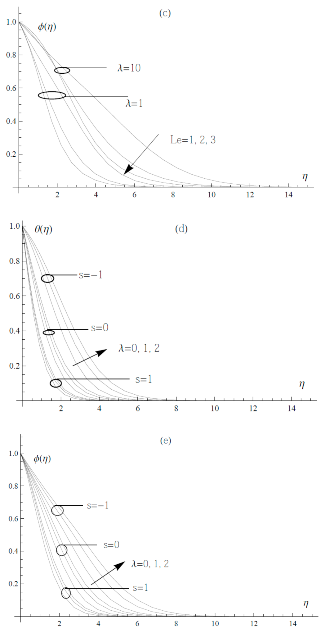
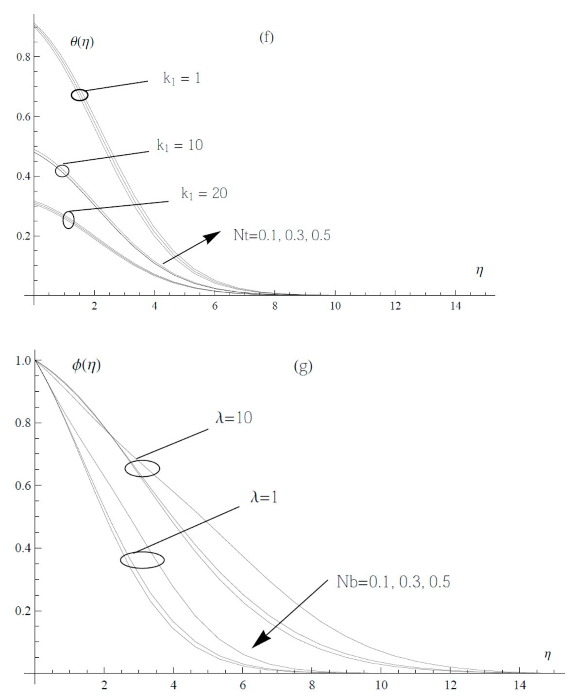
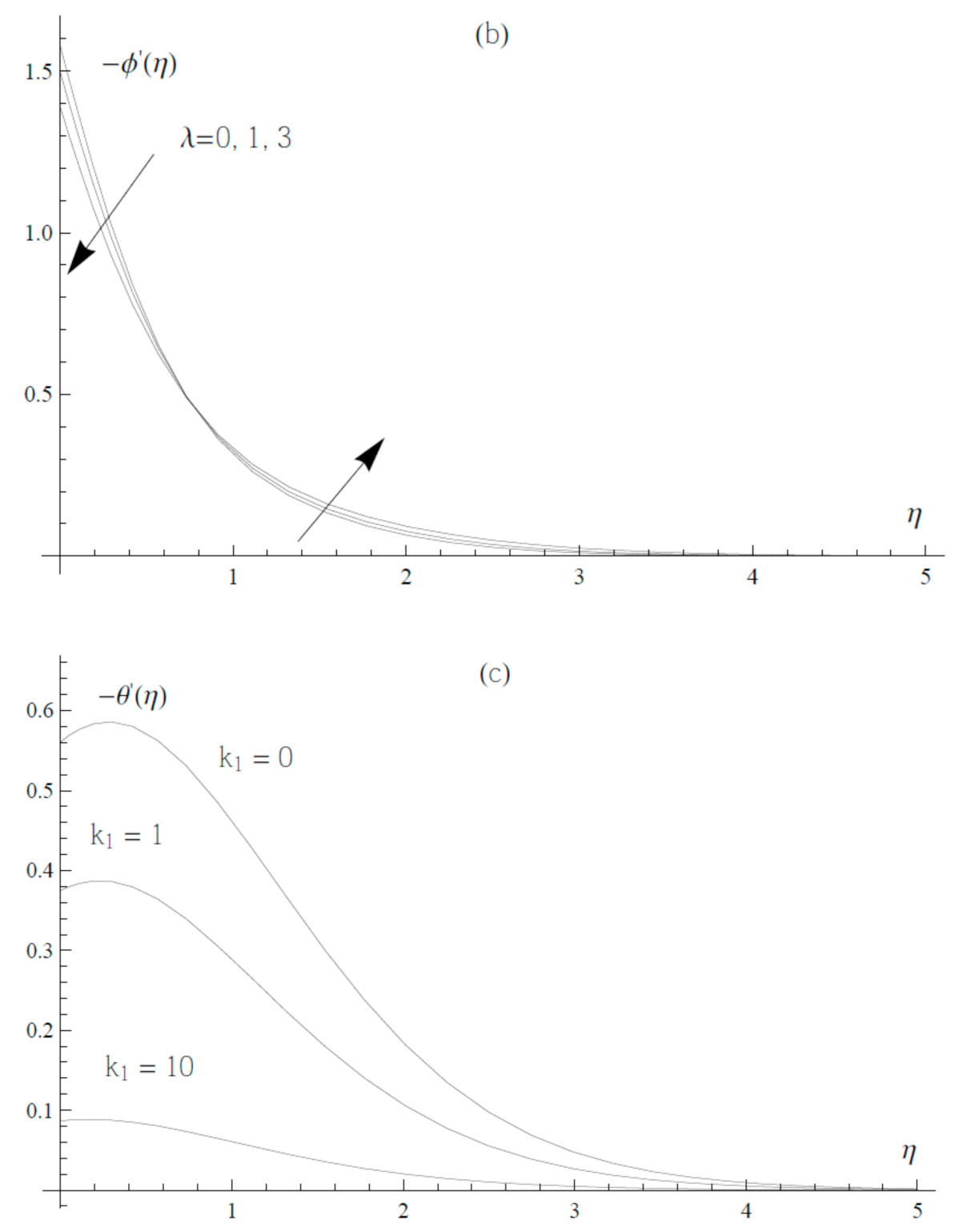
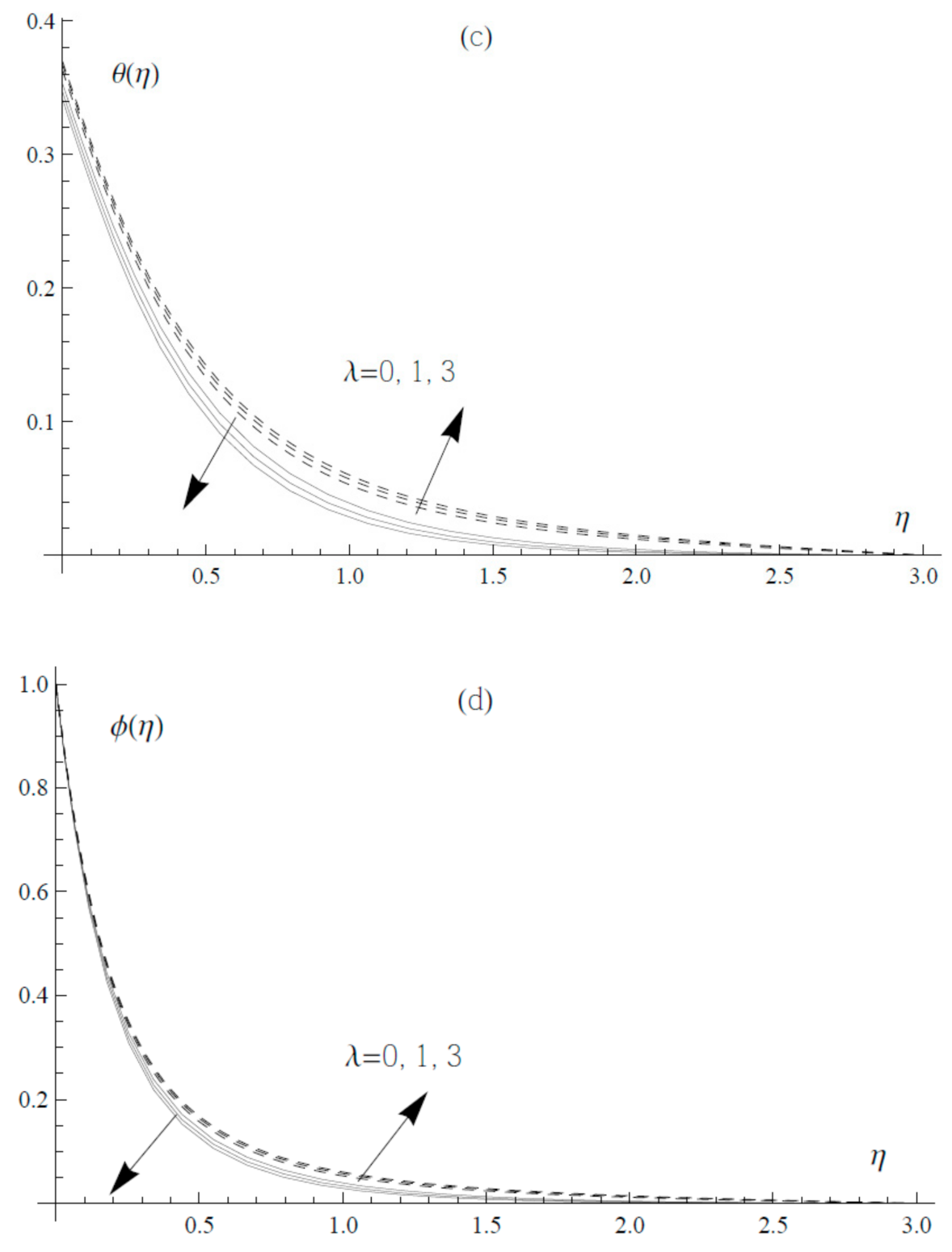
In Figure 2b, both the temperature and concentration profiles are increased by raising the parameter of the slip. It can be seen that a larger Lewis number results in a slower decay of the concentration profile, but it still grows when the slip parameter changes (see Figure 2c). In addition, Figure 2b shows that there are significant differences in the concentration profiles, where with an increase in the parameter of $\lambda =0,1,3$, the concentration profiles increase, but these profiles decrease in the case of $k_1$ changing from $0$ to $20$ (see Figure 3b). Some real examples are provided to back up the claimed simulation findings because of the significance of this discovery for engineers and researchers in almost every field of engineering and science. Such engineering disciplines include nuclear power plants, gas turbines, and different propulsion technologies for airplanes, missiles, satellites, and space vehicles. It is obvious that a larger slip parameter leads to a slower decay of both the temperature and concentration profiles, while an investment effect is seen for the parameters (see Figure 2d,e). Moreover, the thinness of the thermal boundary layer can be observed, for example, in Figure 2f. It is found that with the increasing of $Nb$, the concentration profiles decrease, and the variation of the slip parameter enhances the concentration function, as shown in Figure 2g. Figure 2f,g show the numerical results of the profiles of $\theta \left(\eta \right)$ and $\varphi \left(\eta \right)$ for (f) $k_1=1, 10, 20$ and $\mathrm{Nt}=0.1, 0.3, 0.5 \mathrm{at} \mathrm{Nb}=0.1, \mathrm{Pr}=5, \mathrm{Le}=1, \mathrm{s}=-1,$ and $\lambda =0.01,$ and (g) $\lambda =1, 10$ and $Nb=0.1, 0.3, 0.5$ at $\mathrm{Nt}=0.1, \mathrm{Pr}=5, \mathrm{Le}=1, \mathrm{s}=-1, \mathrm{and} \mathrm{k}₁=0.01$. The temperature function clearly increases as $\mathrm{Nt}$ increases in Figure 2f. However, for varied $\mathrm{Nt}$ and $k_1$ values, the temperature function steadily decreases.

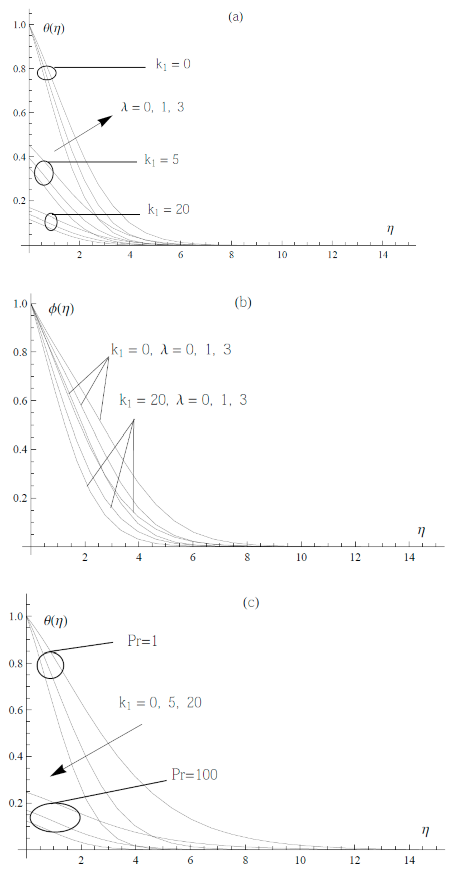
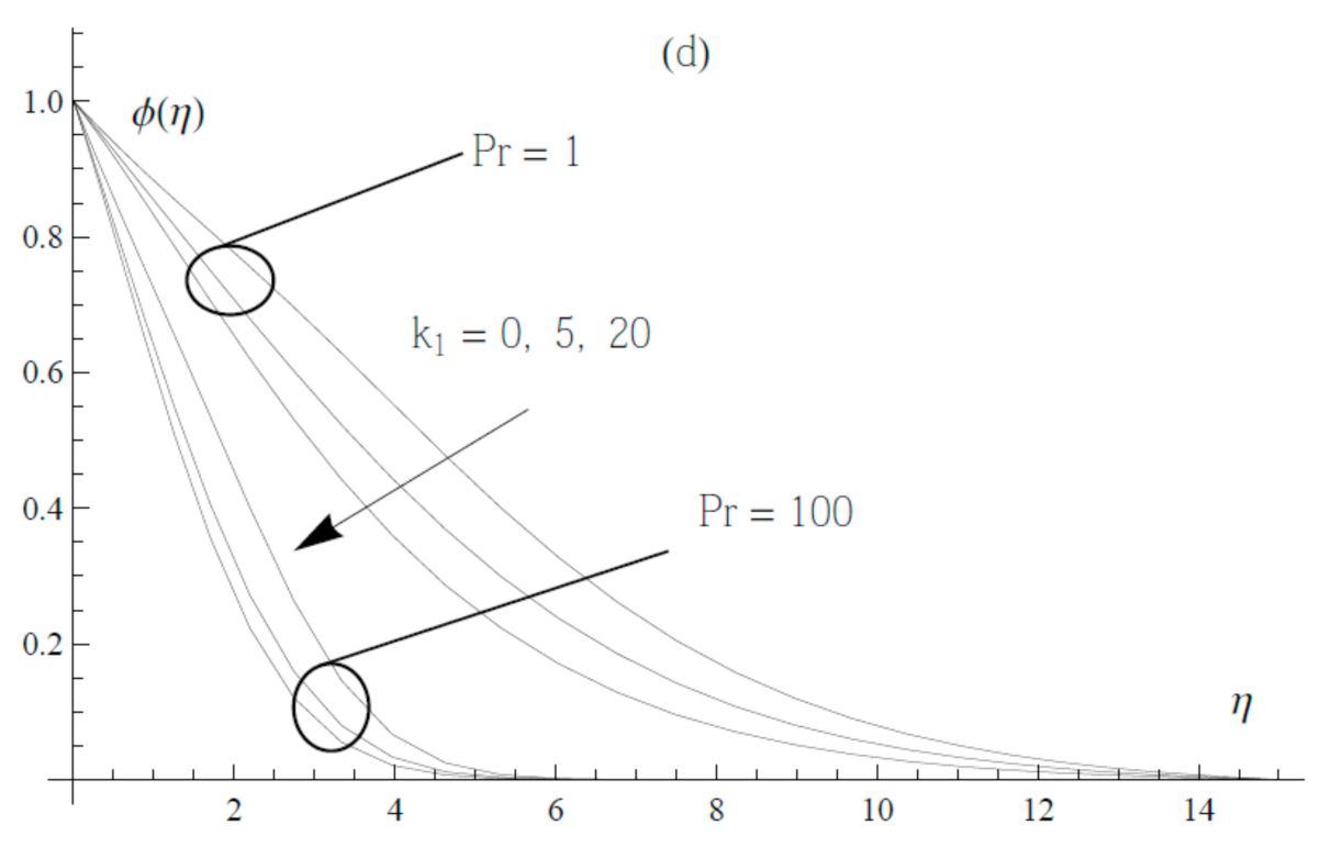
Figure 3 shows the impact of changing various physical parameters ($k_1,\mathsf{\lambda },$ and Pr) on $\theta \left(\eta \right)$ and $\varphi \left(\eta \right).$ Figure 3a,b elucidate the effect of $k_1=0, 5, 20$ and $\mathsf{\lambda }=0, 1, 3 \mathrm{on} \theta \left(\eta \right)$ in (a) and $k_1=0, 20$, $\mathsf{\lambda }=0, 1, 3 \mathrm{on} \varphi \left(\eta \right)$ in (b) for $\mathrm{Nt}=\mathrm{Nb}=0.1, \mathrm{Pr}=5, \mathrm{Le}=1 \mathrm{and} \mathrm{s}=-0.5$. It is evident from Figure 3a that when the parameter $\mathsf{\lambda }$ is increased, the temperature profiles increase and begin at unity near the wall at ${\mathrm{k}}_1=0, \mathsf{\lambda }=0, 1, \mathrm{and} 3$. At varying values of ${\mathrm{k}}_1$ and $\mathsf{\lambda }$, the temperature function $\theta \left(\eta \right)$ decreases rapidly. Temperature profiles diminish, and by raising the parameter of ($\mathrm{Pr}=1, 100$), temperature profiles are reduced, and a thickening of the thermal boundary layer is observed, as shown in Figure 3c. As the Pr value rises, the temperature falls. This is consistent with the physical reality that the thickness of the thermal boundary layer decreases as Pr increases. In Figure 3d, the combination of the ${\mathrm{k}}_1 \mathrm{and} \mathrm{Pr}$ parameters has a significant influence on the concentration profiles. Physically, a higher Prandtl number causes a faster decline in the rate of heat transfer (see [23,25]).

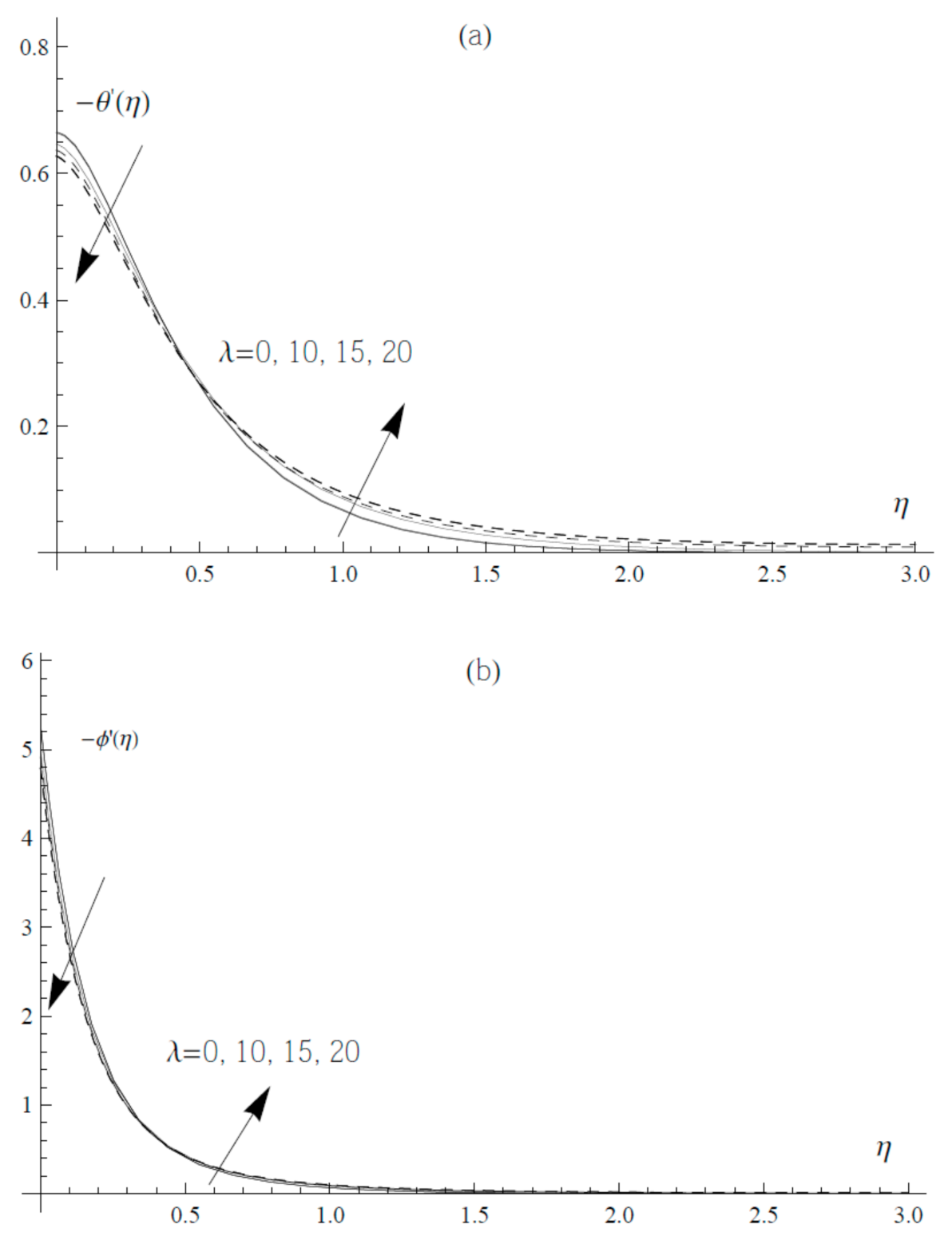
This is due to the fact that a higher Prandtl number indicates lower thermal conductivity and a thinner thermal boundary layer, which reduces the heat transfer rate at the surface. It should be noted that the dimensionless heat transfer rate values exhibit two stages in Figure 4a. Through the first stage, $- \mathsf{\theta }\prime \left(\eta \right)$ can be seen to decline in the domain $0\le \eta \le 1.0$ while $- \mathsf{\theta }\prime \left(\eta \right)$ rising in the domain $1\le \eta \le 5.0,$ indicating that, in this study, fluctuations in the heat transfer rate were reduced near the boundary and increased far away from the border as $\mathsf{\lambda }$ increased. The thickness of the thermal boundary layer for the heat transfer rate, which can be seen in Figure 4a, should be highlighted. In the same vein, Figure 4b depicts two phases of dimensionless mass transfer rate values. Through the first stage, $-{\varphi }^{\prime }\left(\eta \right)$ declined in the domain of $0\le \eta \le 0.8$ while increasing in the domain of $0.8\le \eta \le 5$, indicating that fluctuations in the mass transfer rate were reduced near the border and rose far away from the boundary as $\mathsf{\lambda }$ increased. The thinness of the boundary layer for the mass transfer rate is noticeable in this example. It is worth noting that the temperature jump parameter ${\mathrm{k}}_1$ has a significant influence on the heat transfer rate. However, when ${\mathrm{k}}_1$ increases, the heat transfer rate drops, as seen in Figure 4c [11]. Additionally, it is noted that the boundary layer thickness of the heat transfer rate from ${\mathrm{k}}_1=1 \mathrm{to} 10$ is higher than that of ${\mathrm{k}}_1=0 \mathrm{to} 1$. It is used in thermal engineering, mechanical engineering, and physics for such purposes as heat treatment, ventilation, and air conditioning.

3.2. Shrinking Sheet Results

This section addresses the duality of shrinking sheet solutions for various physical parameter values. Dimensionless similarity functions for the shrinking sheet when $\mathrm{Pr}=10, \mathrm{Le}=1, \mathrm{Nb}=\mathrm{Nt}=0.1, \mathrm{s}=4.5 \mathrm{and} \mathsf{\lambda }={\mathrm{k}}_1=0$ are compared with those obtained in a previous work [23] to assess the precision of our numerical findings, as shown in Figure 5a. It is considered that the shrinking sheet data provided are highly consistent with those given in [23]. Figure 5b shows plots of dual-dimensional similarity functions with $\mathrm{Nb}=\mathrm{Nt}=0.1,\mathrm{Pr}=10,\mathrm{Le}=1, \mathrm{and} \mathrm{s}=4.5,$ in the presence of the slip parameter $\mathsf{\lambda }=1$ and the temperature jump parameter ${\mathrm{k}}_1=0.01$. There is a discrepancy between dimensionless similarity functions $f$ in Figure 5a,b. The dual solutions for the influence of the slip parameter $\mathsf{\lambda }$ on both $\theta \left(\eta \right)$ and $\varphi \left(\eta \right)$ are shown in Figure 5c,d. In the case of the first solution, an increase in the slip parameter leads to a drop in both the temperature function $\theta \left(\eta \right)$ and the concentration function $\varphi \left(\eta \right)$, as well as a decrease in the thermal boundary layer thickness [8,14]. When the slip parameter is changed in the second solution, both the temperature function $\theta \left(\eta \right)$ and the concentration function $\varphi \left(\eta \right)$ decrease.

In addition, the slip parameter has little effect on $\varphi \left(\eta \right)$ and the thickness of the thermal boundary layer. Figure 6a illustrates the dual solutions for the impact of parameter s on $\theta \left(\eta \right).$ Physically, increases in the parameter s slow down the fluid velocity and reduce the temperature and concentration along the sheet [7,23]. Figure 6b,c characterize the dual solutions for the influence of the temperature jump parameter ${\mathrm{k}}_1$ on both $\theta \left(\eta \right)$ and $\varphi \left(\eta \right)$. Raising the parameter ${\mathrm{k}}_1$ lowers both the temperature and the concentration. It can be observed that in the case of the second solution, both the temperature function $\theta \left(\eta \right)$ and the concentration function $\varphi \left(\eta \right)$ are larger than in the case of the first solution.

The dual solutions for the impact of slip and temperature parameters on dimensionless heat and mass transfer rates are shown in Figure 7. It should be noted that with the increasing of $\mathsf{\lambda }$, the dimensionless values of the heat transfer rate showed two stages (see Figure 7a). As $\mathsf{\lambda }$ increased, the variations in the heat transfer rate decreased near the boundary and increased far away from the boundary as follows: $-{\theta }_{\prime }\left(\eta \right)$ was reduced in the domain of $\left(0\le \mathsf{\eta }\le 0.5\right)$ while it rose in the domain of $\left(0.5\le \eta \le 3\right)$. Physically, this indicates that the wall absorbed heat from the fluid at first, but subsequently, the heat progressively dissipated from the wall to the fluid. In the first solution, the temperature gradient was greatest near the surface, which is also where it decreased the most. In addition, the thinness of the thermal boundary layer affected the heat transfer rate. Furthermore, typical matching of the dimensionless mass transfer rate profiles can be observed, as shown in Figure 7b. The thermal boundary layer thickness was higher for the $-{\theta }^{\prime }\left(\eta \right)$ profiles than for the $-{\varphi }^{\prime }\left(\eta \right)$ profiles (see Figure 7c,d). Moreover, the dimensionless mass transfer rate $-{\varphi }^{\prime }\left(\eta \right)$ values exhibit two stages in Figure 7d. $-{\varphi }^{\prime }\left(\eta \right)$ dropped in the domain of $\left(0\le \eta \le 0.35\right)$, whereas it rose in the domain of $\left(0.35\le \eta \le 3\right)$, indicating that variances in the mass transfer rate were reduced near the boundary and increased further away from the boundary as $\mathsf{\lambda }$ increased.

Finally, Figure 8a,b show the fluctuation of dual numerical findings for the reduced Nusselt number and the reduced Sherwood number at various $\mathrm{Nb}$ and $\mathrm{Nt}$ values when values of $\mathrm{Pr}=100, \mathrm{Le}=1, \mathsf{\lambda }= \mathrm{k}₁=1, \mathrm{and} \mathrm{s}=-0.5$ were applied to shrinking sheets. The duals of the reduced Nusselt number and the reduced Sherwood number are both decreasing functions. This has important applications in thermal engineering, mechanical engineering, and physics, such as heat treatment, ventilation, and air conditioning, as well as in renewable energy sources.

4. Conclusions

The effects of the partial slip boundary condition and the jump temperature on nanofluid flow heat and mass transfer over a stretching or shrinking surface were studied. The nanofluid model combines the effects of Brownian motion and thermophoresis. It was found that dual solutions exist for the shrinking case, while the solution is unique for the stretching case. The design of chemical processing equipment, the design of heat exchangers, the formation and dispersion of fog, temperature and moisture distributions over agricultural fields, environmental pollution, and thermo protection systems are some of the applications of interest that use combined heat and mass transfer by natural convection. A system of nonlinear ordinary differential equations was numerically solved using the Chebyshev pseudospectral technique at particular physical parameter values of $\mathrm{Pr}, \mathrm{Nb}, \mathrm{Nt}, \mathrm{Le}, \mathrm{s}, \mathsf{\lambda },$ and ${\mathrm{k}}_1$.

Based on past findings, the following was established:

• It was discovered that when $\mathrm{Pr}=5, \mathrm{Le}=1, \mathrm{and} \mathrm{s}=-0.5$ in the case of stretched sheet, the reduced Nusselt number is a falling function whereas the reduced Sherwood number is a rising function at various values of $\mathrm{Nt}, \mathrm{Nb}, \mathsf{\lambda }, \mathrm{and} {\mathrm{k}}_1$ (see, Table 1). The reverse is true for the shrinking sheet at various values of $\mathrm{Nt}$ and $\mathrm{Nb}$ when $\mathrm{Pr}=100, \mathrm{Le}=1, \mathrm{s}=-0.5, \mathsf{\lambda }=1$, and ${\mathrm{k}}_1=1$, as shown in Figure 8a,b.
• The slip parameter improves the temperature field and increases the thermal boundary layer thickness, as well as the concentration function’s boundary layer thickness in the case of a stretched sheet. On the other hand, in the case of the shrinking sheet, the dual solutions for temperature and concentration functions are lowered when the slip parameter is increased. Both temperature and concentration functions were found to decrease with the increasing of the slip parameter for the first solution, whereas both the temperature and concentration functions were found to increase with the increasing of the slip parameter for the second solution (see Figure 5c,d). In this situation, the influence of $\mathsf{\lambda }$ on both the temperature and concentration profiles is greater for the first solutions than for the second solutions.
• The temperature jump parameter ${\mathrm{k}}_1$ has a significant impact on temperature and concentration profiles. As shown in Figure 3c,d for stretching sheets and Figure 6c,d for shrinking sheets, increasing the temperature jump parameter ${\mathrm{k}}_1$ causes the temperature and concentration profiles to decline.
• Heat and mass transfer rates become monotone as the slip parameter increases, as seen in Figure 4a,b for the stretching sheet and Figure 7a for the shrinking sheet. Furthermore, the slip parameter has no effect on the mass transfer rate of the shrinking sheet (see Figure 7b).
• The thickness of the thermal boundary layer of the heat transfer rate rises as the temperature jump parameter $\mathrm{k}₁$ increases, as seen in Figure 4c and Figure 7c for both stretching and shrinking sheets, thereby reducing the heat transfer rate.
• The findings have potential uses in a variety of fields, particularly in the optimal design of a solar energy collector’s heat transfer.

References

- Buongiorno, J. Convective Transport in Nanofluids. J. Heat Transf. 2005, 128, 240–250. [Google Scholar] [CrossRef]
- Eastman, J.A.; Choi, S.U.S.; Li, S.; Yu, W.; Thompson, L.J. Anomalously increased effective thermal conductivities of ethylene glycol-based nanofluids containing copper nanoparticles. Appl. Phys. Lett. 2001, 78, 718–720. [Google Scholar] [CrossRef]
- Gupta, A.K.; Gupta, M. Synthesis and surface engineering of iron oxide nanoparticles for biomedical applications. Biomaterials 2005, 26, 3995–4021. [Google Scholar] [CrossRef] [PubMed]
- Keblinski, P.; Phillpot, S.; Choi, S.; Eastman, J. Mechanisms of heat flow in suspensions of nano-sized particles (nanofluids). Int. J. Heat Mass Transf. 2002, 45, 855–863. [Google Scholar] [CrossRef]
- Xiong, Q.; Altnji, S.; Tayebi, T.; Izadi, M.; Hajjar, A.; Sundén, B.; Li, L.K. A comprehensive review on the application of hybrid nanofluids in solar energy collectors. Sustain. Energy Technol. Assess. 2021, 47, 101341. [Google Scholar] [CrossRef]
- Aneli, S.; Gagliano, A.; Tina, G.M.; Hajji, B. Analysis of the energy produced and energy quality of nanofluid impact on photovoltaic-thermal systems. In Proceedings of the 2020 ICEERE 2nd International Conference on Electronic Engineering and Renewable Energy Systems, Saidia, Morocco, 13–15 April 2020; pp. 739–745. [Google Scholar]
- Elgazery, N.S.; Elelamy, A.F. Multiple solutions for non-Newtonian nanofluid flow over a stretching sheet with nonlinear thermal radiation: Application in transdermal drug delivery. Pramana 2020, 94, 1–22. [Google Scholar] [CrossRef]
- Ghosh, S.; Mukhopadhyay, S.; Vajravelu, K. Dual solutions of slip flow past a nonlinearly shrinking permeable sheet. Alex. Eng. J. 2016, 55, 1835–1840. [Google Scholar] [CrossRef] [Green Version]
- Rana, P.; Dhanai, R.; Kumar, L. Radiative nanofluid flow and heat transfer over a non-linear permeable sheet with slip conditions and variable magnetic field: Dual solutions. Ain Shams Eng. J. 2017, 8, 341–352. [Google Scholar] [CrossRef] [Green Version]
- Bhattacharyya, K. Dual solutions in boundary layer stagnation-point flow and mass transfer with chemical reaction past a stretching/shrinking sheet. Int. Commun. Heat Mass Transf. 2011, 38, 917–922. [Google Scholar] [CrossRef]
- Soid, S.K.; Ishak, A.; Pop, I. Unsteady MHD flow and heat transfer over a shrinking sheet with ohmic heating. Chin. J. Phys. 2017, 55, 1626–1636. [Google Scholar] [CrossRef]
- Bhargava, R.; Chandra, H. Numerical simulation of MHD boundary layer flow and heat transfer over a nonlinear stretching sheet in the porous medium with viscous dissipation using hybrid approach. J. Arxiv Fluid Dyn. 2017, 17, 1–19. [Google Scholar]
- Reddy, J.V.R.; Sugunamma, V.; Sandeep, N. Simultaneous impacts of Joule heating and variable heat source/sink on MHD 3D flow of Carreau-nanoliquids with temperature dependent viscosity. Nonlinear Eng. 2018, 8, 356–367. [Google Scholar] [CrossRef]
- Mansur, S.; Ishak, A.; Pop, I. Flow and heat transfer of nanofluid past stretching/shrinking sheet with partial slip boundary conditions. Appl. Math. Mech. 2014, 35, 1401–1410. [Google Scholar] [CrossRef]
- Mousavi, S.M.; Dinarvand, S.; Yazdi, M.E. Generalized second-order slip for unsteady convective flow of a nanofluid: A utilization of Buongiorno’s two-component nonhomogeneous equilibrium model. Nonlinear Eng. 2020, 9, 156–168. [Google Scholar] [CrossRef]
- Acharya, N.; Bag, R.; Kundu, P.K. Unsteady bioconvective squeezing flow with higher-order chemical reaction and second-order slip effects. Heat Transf. 2021, 50, 5538–5562. [Google Scholar] [CrossRef]
- Noghrehabadi, A.; Pourrajab, R.; Ghalambaz, M. Effect of partial slip boundary condition on the flow and heat transfer of nanofluids past stretching sheet prescribed constant wall temperature. Int. J. Therm. Sci. 2012, 54, 253–261. [Google Scholar] [CrossRef]
- Khan, M.; Rasheed, A. Slip velocity and temperature jump effects on molybdenum disulfide MoS2 and silicon ox-ide SiO2 hybrid nanofluid near irregular 3D surface. Alex. Eng. J. 2021, 60, 1689–1701. [Google Scholar] [CrossRef]
- Canuto, C.; Hussaini, M.Y.; Zang, T.A. Spectral Methods in Fluid Dynamic; Springer: New York, NY, USA, 1988. [Google Scholar]
- Peyret, R. Spectral Methods for Incompressible Viscous Flow; Springer: New York, NY, USA, 2002. [Google Scholar]
- Elbarbary, E.M.E.; El-Sayed, S.M. Higher-order pseudospectral differentiation matrices. Appl. Numer. Math. 2005, 55, 425–438. [Google Scholar] [CrossRef]
- Abd Elazem, N.Y. Numerical results for influence the flow of MHD nanofluids on heat and mass transfer past a stretched surface. Nonlinear Eng. 2021, 10, 28–38. [Google Scholar] [CrossRef]
- Abd Elazem, N.Y. Numerical Solution for the Effect of Suction or Injection on Flow of Nanofluids Past a Stretching Sheet. Z. Nat. A 2016, 71, 511–515. [Google Scholar] [CrossRef]
- Kuznetsov, A.V.; Nield, D.A. Natural convective boundary-layer flow of a nanofluid past a vertical plate. Int. J. Therm. Sci. 2010, 49, 243–247. [Google Scholar] [CrossRef]
- Khan, W.A.; Pop, I. Boundary-layer flow of a nanofluid past a stretching sheet. Int. J. Heat Mass Transf. 2010, 53, 2477–2483. [Google Scholar] [CrossRef]
- Naveed, M.; Awais, M.; Abbas, Z.; Sajid, M. Analysis of Joule heating in a chemically reactive flow of time dependent Carreau-nanofluid over an axisymmetric radially stretched sheet using Cattaneo-Christov heat flux model. Ric. Mat. 2021. [Google Scholar] [CrossRef]
- Suganya, S.; Muthtamilselvan, M.; Abdalla, B. Effects of radiation and chemical reaction on Cu-Al2O3/water hybrid flow past a melting surface in the existence of cross magnetic field. Ric. Mat. 2021. [Google Scholar] [CrossRef]
- Dan, D.D.; Zhang, W.; Wang, Y.L.; Ban, T.T. Using piecewise reproducing kernel method and Legendre polynomial for solving a class of the time variable fractional order advection-reaction-diffusion equation. Therm. Sci. 2021, 25, 1261–1268. [Google Scholar]
- Tian, Y.; Liu, J. Direct algebraic method for solving fractional Fokas equation. Therm. Sci. 2021, 25, 2235–2244. [Google Scholar] [CrossRef]
- Tian, D.; Ain, Q.T.; Anjum, N.; He, C.H.; Cheng, B. Fractal N/MEMS: From pull-in instability to pull-in stability. Fractals 2021, 29, 2150030. [Google Scholar] [CrossRef]
- Tian, D.; He, C.H. A fractal micro-electromechanical system and its pull-in stability. J. Low Freq. Noise Vib. Act. Control 2021, 1461348420984041. [Google Scholar] [CrossRef]
- He, C.H.; Tian, D.; Moatimid, G.M.; Salman, H.F.; Zekry, M.H. Hybrid Rayleigh-van der pol-duffing oscillator: Stability analysis and controller. J. Low Freq. Noise Vib. Act. Control 2021, 14613484211026407. [Google Scholar] [CrossRef]
- Liu, F.; Zhang, T.; He, C.H.; Tian, D. Thermal oscillation arising in a heat shock of a porous hierarchy and its application. Facta Univ. Ser. Mech. Eng. 2021. [Google Scholar] [CrossRef]
Figure 1.
Physical diagram of the flow geometry.
Figure 2.
(a) Comparison of the dimensionless similarity function θ(η) when Pr = Le = 1, Nb = Nt = 0.1, s = 0.1, and λ = k1 = 0 for the stretching sheet in the present study with the results obtained in ref. Abd Elazem [23] (the continuous line represents the present results; the dots are from Ref [23]). (b) Effect of λ on θ(η) and Φ(η) at Nt = Nb = 0.1, Pr = 5, Le = 1, s = 0.8, and k1 = 0.01 for the stretching sheet. (c) Effect of λ and Le on Φ(η) at Nt = Nb = 0.1, Pr = 5, s = −0.8, and k1 = 0.01 for the stretching sheet. (d) Effect of λ and s on θ(η) at Nt = Nb = 0.1, Pr = 5, Le = 1, and k1 = 0.01 for the stretching sheet. (e) Effect of λ and s on Φ(η) at Nt = Nb = 0.1, Pr = 5, Le = 1, and k1 = 0.01 for the stretching sheet. (f) Effect of k1 and Nt on θ(η) at Nb = 0.1, Pr = 5, Le = 1, s = −1, and λ = 3 for the stretching sheet. (g) Effect of λ and Nb on Φ(η) at Nt = 0.1, Pr = 5, Le = 1, s = −1, and k1 = 0.01 for the stretching sheet.
Figure 3.
(a) Effect of k1 and λ on θ(η) at Nt = Nb = 0.1, Pr = 5, Le = 1, and s = −0.5 for the stretching sheet. (b) Effect of k1 and λ on Φ(η) at Nt = Nb = 0.1, Pr = 5, Le = 1, and s = −0.5 for the stretching sheet. (c) Effect of k1 and Pr on θ(η) at Nt = Nb = 0.1, Le = 1, s = −0.5, and λ = 3 for the stretching sheet. (d) Effect of k1 and Pr on Φ(η) at Nt = Nb = 0.1, Le = 1, s = −0.5, and λ = 3 for the stretching sheet.
Figure 4.
(a) Effect of λ on −θ’(η) at Nt = Nb = 0.5, Pr = 100, Le = 2, s = 0.8, and k1 = 1 for the stretching sheet. (b) Effect of λ on −Φ’(η) at Nt = Nb = 0.5, Pr = 100, Le = 2, s = 0.8, and k1 = 1 for the stretching sheet. (c) Effect of k1 on −θ’(η) at Nt = Nb = 0.5, Pr = 100, Le = 2, s = 0.8, and λ = 1 for the stretching sheet.
Figure 5.
(a) Comparison of the dual dimensionless similarity functions f(η), θ(η), and Φ(η) when Pr = 10, Le = 1, Nb = Nt = 0.1, s = 4.5, and λ = k1 = 0 for the shrinking sheet in the present study with the results obtained in ref. Abd Elazem [23]. (the continuous line represents the present results; the dots are from Ref [23]). (b) Plots of dual dimensionless similarity functions f(η), θ(η), and Φ(η) at Pr = 10, Le = 1, Nb = Nt = 0.1, s = 4.5 when λ = 1, and k1 = 0.01 for the shrinking sheet. (the continuous and the dashed lines represent the first and the second solutions). (c) Dual solutions for the effect of λ on θ(η) at Nb = Nt = 0.5, Pr = 100, Le = 2, s = 4, and k1 = 1 for the shrinking sheet. (the continuous and the dashed lines represent the first and the second solutions). (d) Dual solutions for the effect of λ on Φ(η) at Nb = Nt = 0.5, Pr = 100, Le = 2, s = 4, and k1 = 1 for the shrinking sheet. (the continuous and the dashed lines represent the first and the second solutions).
Figure 6.
(a) Dual solutions for the effect of s on θ(η) at Nt = Nb = 0.5, Pr = 100, Le = 2, s = 4, λ = 3, and k1 = 1 for the shrinking sheet. (the continuous and the dashed lines represent the first and the second solutions). (b) Dual solutions for the effect of k1 on θ(η) at Nb = Nt = 0.5, Pr = 100, Le = 2, s = 4, and λ = 3 for the shrinking sheet. (the continuous and the dashed lines represent the first and the second solutions). (c) Dual solutions for the effect of k1 on Φ(η) at Nb = Nt = 0.5, Pr = 100, Le = 2, s = 4, and λ = 3 for the shrinking sheet. (the continuous and the dashed lines represent the first and the second solutions).
Figure 7.
(a) Dual solutions for the effect of λ on at Nt = Nb = 0.5, Pr = 100, Le = 2, s = 4, and k1 = 1 for the shrinking sheet. (the continuous and the dashed lines represent the first and the second solutions). (b) Dual solutions for the effect of λ on at Nb = Nt = 0.5, Pr = 100, Le = 2, s = 4, and k1 = 1 for the shrinking sheet. (the continuous and the dashed lines represent the first and the second solutions). (c) Dual solutions for the effect of k1 on at Nb = Nt = 0.5, Pr = 100, Le = 2, s = 4, and λ = 3 for the shrinking sheet. (the continuous and the dashed lines represent the first and the second solutions). (d) Dual solutions for the effect of k1 on at Nb = Nt = 0.5, Pr = 100, Le = 2, s = 4, and λ = 3 for the shrinking sheet. (the continuous and the dashed lines represent the first and the second solutions).
Figure 8.
(a) Dual solutions for the effect of Nt on at various values of Nb when Pr = 100, Le = 1, s = −0.5, λ = 1, and k1 = 1 for the shrinking sheet. (the continuous and the dashed lines represent the first and the second solutions). (b) Dual solutions for the effect of Nt on at various values of Nb when Pr = 100, Le = 1, s = −0.5, λ = 1, and k1 = 1 for the shrinking sheet (the continuous and the dashed lines represent the first and the second solutions).