
Control-Oriented Modeling for Nonlinear MIMO Turbofan Engine Based on Equilibrium Manifold Expansion Model

1
School of Energy Science and Engineering, Harbin Institute of Technology, No. 92, West Da-Zhi Street, Harbin 150001, China
2
Shenyang Airplane Design and Research Institution, Shenyang 110013, China
3
Xi’an Aerospace Propulsion Institute, Xi’an 710199, China
*
Author to whom correspondence should be addressed.
Energies 2021, 14(19), 6277; https://doi.org/10.3390/en14196277
Submission received: 10 August 2021
/
Revised: 8 September 2021
/
Accepted: 17 September 2021
/
Published: 2 October 2021
(This article belongs to the Topic Optimisation, Optimal Control and Nonlinear Dynamics in Electrical Power, Energy Storage and Renewable Energy Systems)
Abstract
:This paper investigates the control-oriented modeling for turbofan engines. The nonlinear equilibrium manifold expansion (EME) model of the multiple input multiple output (MIMO) turbofan engine is established, which can simulate the variation of high-pressure rotor speed, low-pressure rotor speed and pressure ratio of compressor with fuel flow and throat area of the nozzle. Firstly, the definitions and properties of the equilibrium manifold method are presented. Secondly, the steady-state and dynamic two-step identification method of the MIMO EME model is given, and the effects of scheduling variables and input noise on model accuracy are discussed. By selecting specific path, a small amount of dynamic data is used to identify a complete EME model. Thirdly, modeling and simulation at dynamic off-design conditions show that the EME model has model accuracy close to the nonlinear component-level (NCL) model, but the model structure is simpler and the calculation is faster than that. Finally, the linearization results are obtained based on the properties of the EME model, and the stability of the model is proved through the analysis of the eigenvalues, which all have negative real parts. The EME model constructed in this paper can meet the requirements of real-time simulation and control system design.
1. Introduction
In recent years, as an ideal power plant for aircraft, turbofan engine has received extensive attention [1,2,3,4,5]. The continuous improvement of aircraft performance and the expansion of flight envelope have put forward higher requirements for the control system of turbofan engines. Data show that 80% of the work for the aero-engine control system design is devoted to modeling and understanding the characteristics of engine [6]. Therefore, control-oriented modeling plays a significant role in the design. However, the turbofan engine is a complex aerodynamic thermodynamic system with multi-variable, nonlinear, and time-varying characteristics, so the control-oriented modeling of the turbofan engine faces great challenges.
The modeling needs to resolve the contradiction between model accuracy and real-time. Early work on aero-engine modeling is to build nonlinear component-level (NCL) models [7,8,9]. The input-output relationships are established based on the characteristics of each component of the turbofan engine. Then, the NCL model is established according to the relationship and various constraints. At present, the NCL model has been applied in real-time simulation and used to complete the real-time digital verification of the control system [10,11]. However, the NCL model cannot meet the requirements of the closed-loop control system design for the turbofan engine due to its complexity [12]. Since most modern control methods are based on linear theory, the state variable model is often used in linear system theory. It is a linear model established in the state space, which can be obtained by derivative method [13] and fitting method [14,15]. Unfortunately, although the state variable model solves the application of linear control method in turbofan engines, it only has good fitting effect near the steady-state point used in the model identification. This shows that the state variable model is not effective for a wide range of operating conditions. At the same time, it is difficult to guarantee the good performance of turbofan engines in full envelope or in a wide range of operating conditions. In order to deal with these problems, the linear parameters-varying (LPV) model has been widely discussed in academia [16]. The modeling methods of LPV and quasi-LPV are discussed in Refs. [16,17], and the main difference between them is that quasi-LPV considers the change of state variables. There are three main modeling methods for the LPV model: the Jacobian linearization approach [18], the state transformations techniques [19], and the function substitution method [20]. Huang et al. [21] studied the identification of the LPV model with two scheduling variables. Rotondo et al. [22] introduced the modeling of the quasi-LPV for MIMO system. Lu and Huang [23] proposed a new lifecycle real-time model to describe the dynamic behavior of turbofan engines and studied engine/model mismatch compensation and performance degradation adaptive problems. The LPV model was converted to a switched convex polytopic form with hysteresis switching logic, and a switched LPV model of aero-engine rotor speed was obtained in Ref. [24]. With the development of LPV technology, many studies have appeared on the control method of turbofan engines in a wide range of operating conditions. However, the main problem of LPV method is that equilibrium points of engines change greatly with the scheduling variable in the actual work process, which brings great challenges to the accuracy and stability of the LPV model.
In order to obtain a control-oriented model that guarantees the accuracy and stability in a wide range of working conditions, the equilibrium manifold expansion (EME) model is proposed [25,26,27,28,29]. The ultimate goal of the equilibrium manifold method is to obtain the linearized family of nonlinear plants expanded along the equilibrium manifold. Thus, the EME model contains steady-state and dynamic characteristics of the nonlinear system near the equilibrium manifold, which are beneficial for the modeling of turbofan engines with operating line. Different from the LPV model, the EME model considers the mapping between the EM and scheduling variables, thereby ensuring the high accuracy of the model. Moreover, the equilibrium manifold method has been well applied in the modeling of areo-engines. The comparison of simulation and engineering test data has a small error. Yu et al. [25] studied the design of the shock position control system based on the equilibrium manifold method. Sui and Yu [26] proposed the EME model, analyze the error of the model, and solve the ill-posed problem of the identification matrix by using the constraint conditions of the equilibrium manifold. Yu and Zhao [27,28] developed the aero-engine control based on the EME model, and establish the affine EME model to complete the feedback linearization control of the engine. Liu et al. [29,30] built a control-oriented surge margin EME model and discussed the adaptive problem based on the EME model. In order to further improve the accuracy of the EME model, a switched EME model was proposed, and the switching control of the aircraft engine was carried out after the stability was proven [31]. Chen and Zhao [32] applied the switching control to the acceleration and safety protection of turbofan engines based on the switched EME model. With the improvement of the performance requirements for turbofan engine, the engine must be developed in a geometrically adjustable direction to ensure both performance and safety. Unfortunately, the aforementioned EME models are identified from the SISO systems with fuel flow as an input variable, which cannot meet the control requirements of advanced turbofan engines in a wide range of working conditions. In particular, geometrically adjustable variables, such as throat area of the nozzle, expand the operating range of turbofan engines. Up to now, few studies about how to extend the EME model from SISO system to MIMO system have been reported. Therefore, constructing the MIMO EME mode of turbofan engine is a new perspective, which is the focus of this paper.
Compared with existing studies, the main contributions of this work are as follows. Firstly, the basic definition of EM and EME model is introduced in Section 2, and the mathematical properties of the EME model are given. Subsequently, the modeling of the EME model for MIMO turbofan engine is given in Section 3. The steady-state and dynamic data needed for the identification of the MIMO EME model are obtained through the NCL model simulation, and all the parameters are normalized. After constructing the EME model, the EME model of the MIMO turbofan engine is obtained by using the steady-state and dynamic two-step identification method. In the process of dynamic parameter identification, it is creatively proposed to use less identification data and discuss the influence of different paths on dynamic parameter identification. In addition, the EME model shows that it can ensure the recognition accuracy under the interference of input noise. The EME models of the MIMO turbofan engine with different scheduling variables are discussed. Besides, the validation and stability analysis of the EME model is stated in Section 4. This paper verifies the accuracy of the EME model at off-design points. The validity and reliability of EME model is demonstrated over the whole range of operating conditions. In addition, the stability analysis of the EME model is carried out based on the linearization results of the model. Finally, Section 5 presents conclusion.
2. Description of EM and EME Model
2.1. Definitions of the Model
Consider the nonlinear system in the following form:
where is the state variable, is the input variable, is the output variable, and and are corresponding smooth nonlinear functions.
Definition 1
The EM which contains a series of algebraic equations is parameterized by the scheduling variable . Generally, the dimensional of scheduling variable is equal to the dimensional of input variable u, and the scheduling variable is selected from the steady-state value of input or state variables. Therefore, all the equations of the EM can be expressed as the functions of , namely:
Definition 2
(Ref. [27]). The equilibrium manifold expansion (EME) model of system (1) is a family of first-order Taylor expansion at different equilibrium points , and there appears a mapping between the scheduling variable and current operating point . The EME model is expressed as:
where the content in Equation (4) can be simplified as:
The research shows that the mapping is not arbitrary [26]. It must satisfy the condition that any equilibrium point maps to itself. That is, must be satisfied in the mapping. Although the EME model of system (1) is obtained by Taylor expansion, it is still a nonlinear system when the scheduling variable is eliminated.
2.2. Properties of the Model
There are a lot of studies on equilibrium manifold modeling in SISO aircraft gas turbine engine. Compared with other models, the EME model has advantages in accuracy and real-time performance due to its property.
Property 1.
The linearization results and the EME model (4) of nonlinear system (1) are the same at any equilibrium point [27].
Explanation:The EME model can be regarded as an approximate nonlinear result of system (1), which is valid only if the linearization results of the two are consistent. At the same steady state, the coefficient matrix , , , and should be consistent.
Property 2.
Equation (6) is a necessary and sufficient condition for EM (2) to become a family of linearized models [27].
Explanation:Equation (6) is the constraint of the steady-state and dynamic structure of the EME model. The unique identification method and structure of the EME model may result in missing parameters of Equation (5). Therefore, the completeness of linearization results of the EME model can be guaranteed by the constraint of Equation (6).
3. Modeling of the EME Model for the MIMO Turbofan Engines
3.1. The Source of the Identification Data
In order to identify the EME model of the turbofan engine, it is necessary to carry out the simulation in a wide range of operating conditions. The NCL model used in this paper was established by Ref. [33]. A high degree of confidence component level model of a twinspool turbofan engine has been achieved. The turbofan engine mainly consists of the following components: inlet, fan, HPC, combustor, High Pressure Turbine (HPT), Low Pressure Turbine (LPT), bypass, and nozzle. Each component is modeled by aerothermodynamics calculations and solving a set of balance equations. The engine design operation data and characteristic maps of rotating components are used to construct the turbofan engine nonlinear model [34]. This NCL model of turbofan engine has been used in other studies [35,36,37,38]. The NCL model only provides the raw data needed for the EME model identification. Through the study of EME model identification methods, the high-precision mathematical models that can fit different types of turbofan engines will be obtained.
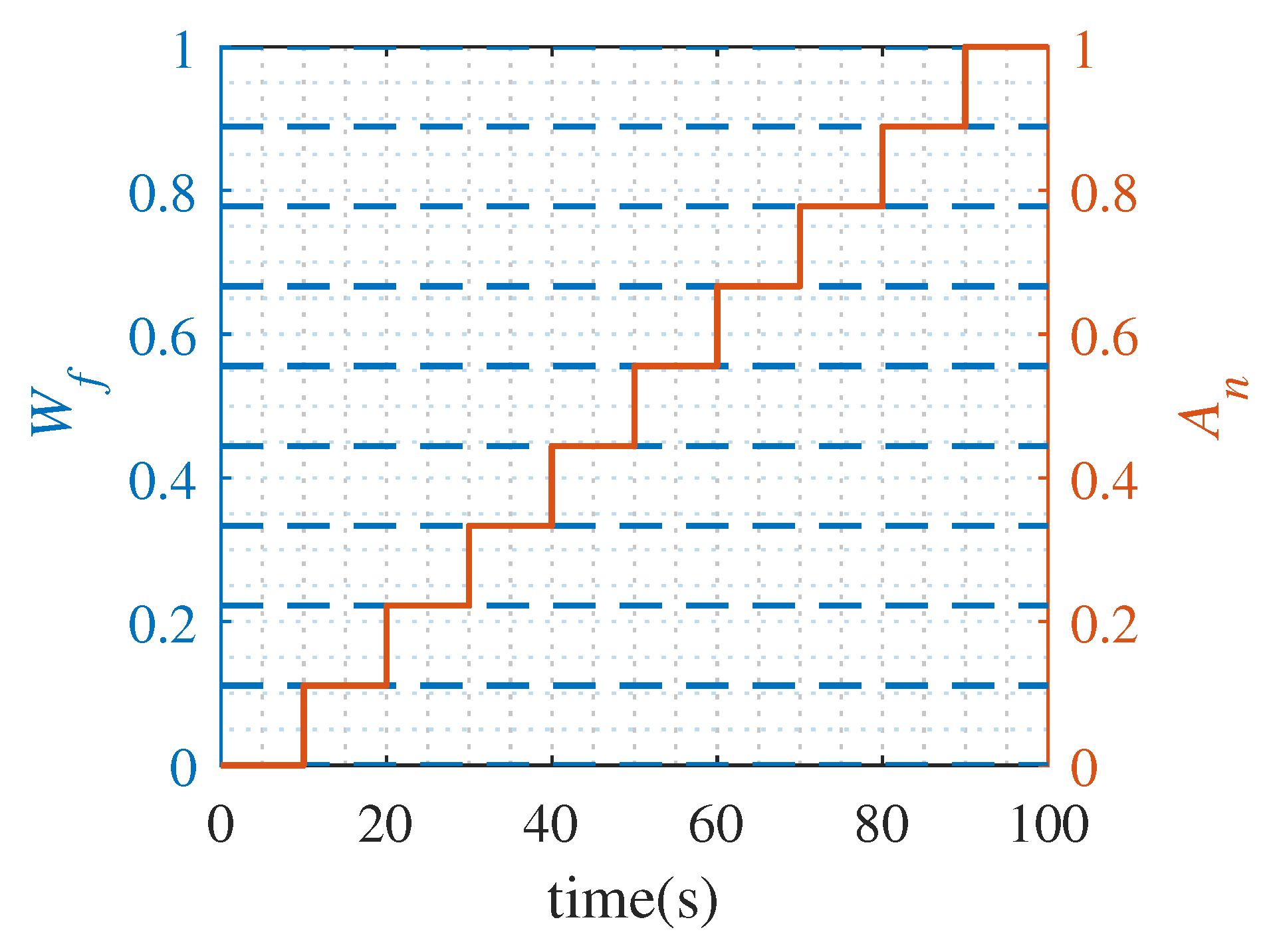
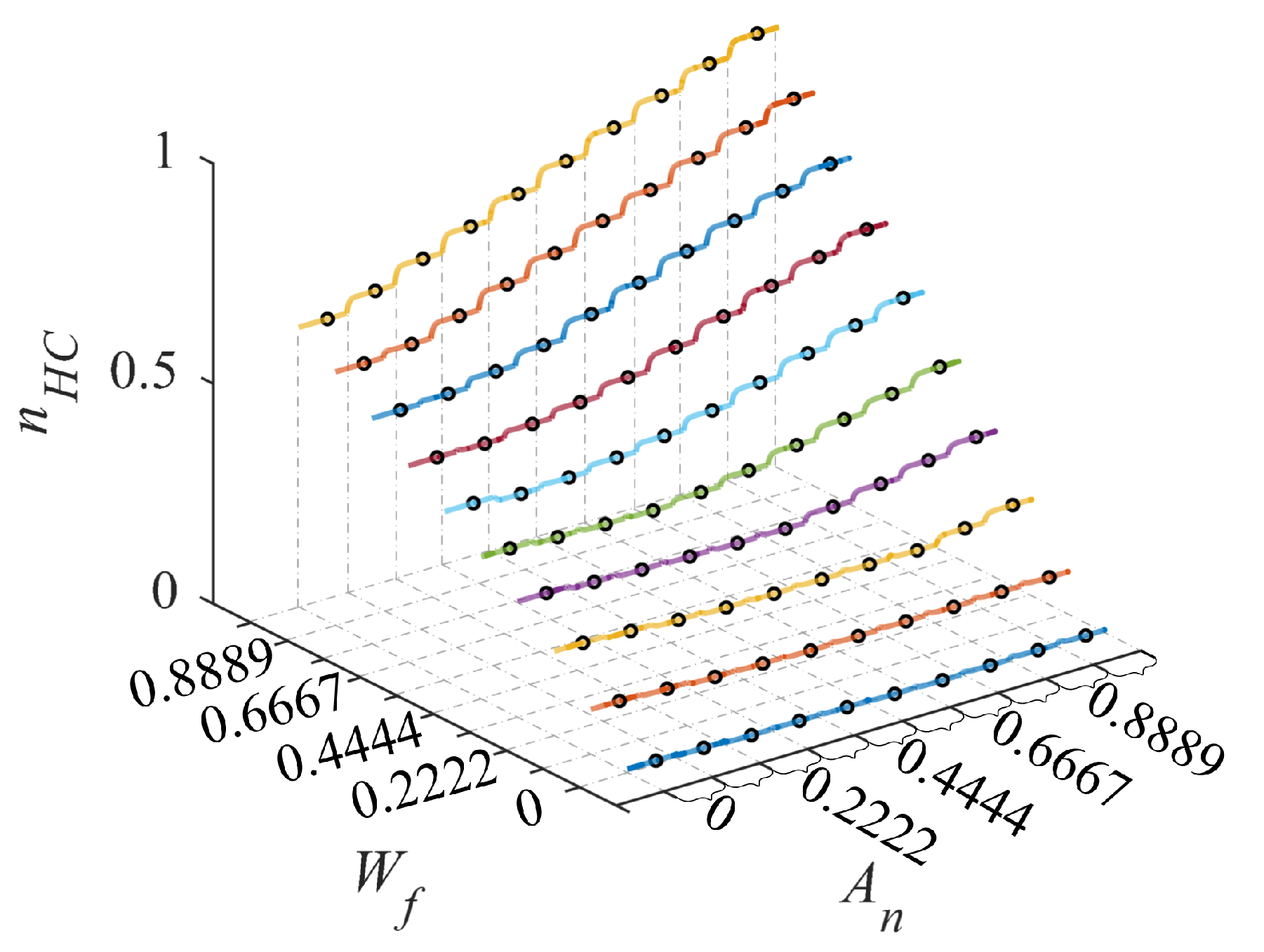
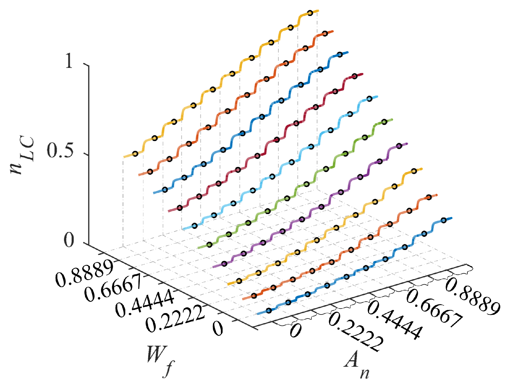
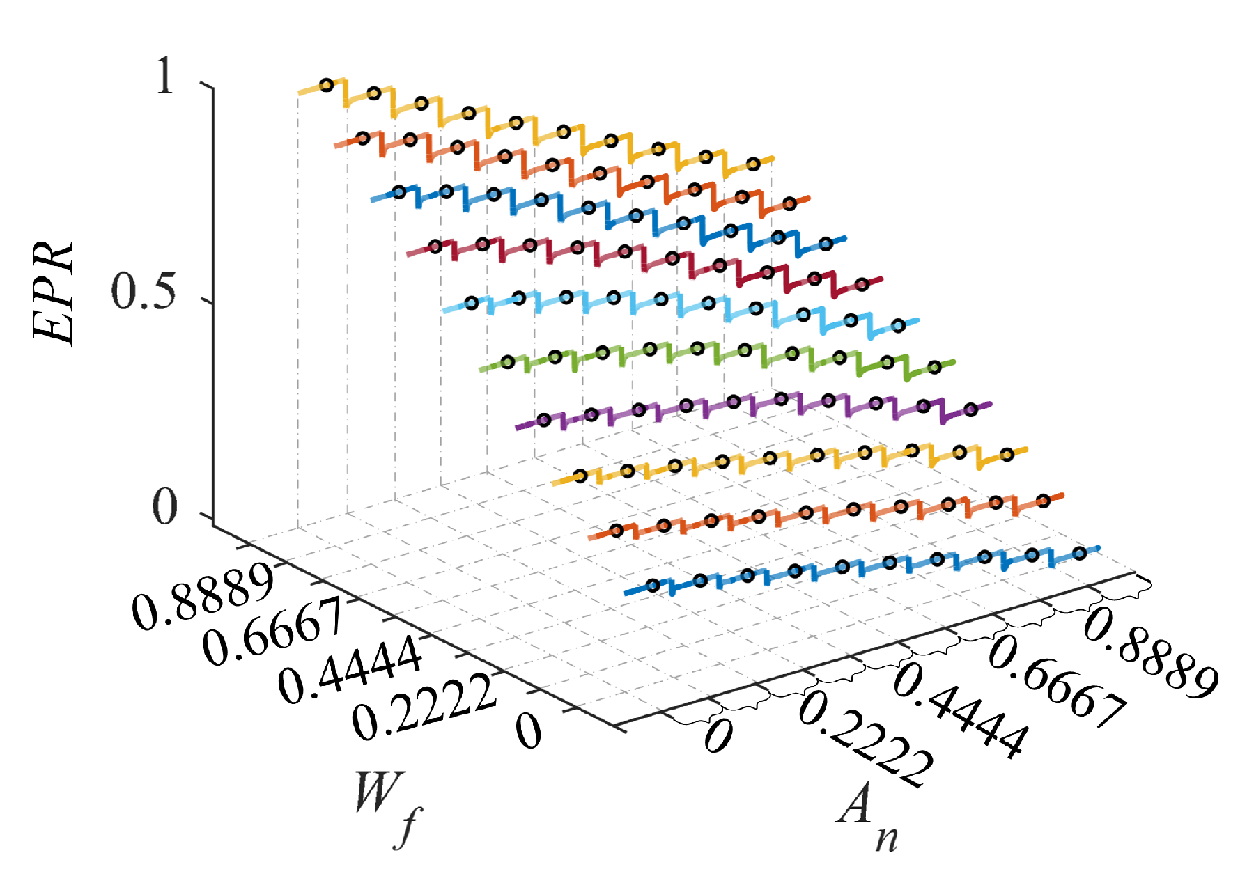
The EM of an MIMO turbofan engine develops from a simple curve to a complex surface form. In the simulation, the engine NCL model works at H = 0 km, Ma = 0. In this paper, input variables of MIMO turbofan engine are fuel flow and throat area of the nozzle . At each , the increases step by step during simulation. The specific change of input variables is shown in Figure 1. Then, the high-pressure rotor speed , low-pressure rotor speed , and engine pressure ratio () are considered to be the output variables of the turbofan engine. Figure 2, Figure 3 and Figure 4 show the output results of the NCL model in simulation. The inputs in Figure 1 is normalized, and the actual range of is 1.5906–2.4060 kg/s, while the actual range of is 0.2577–0.3144 . This process involves the acceleration of the engine. Meanwhile, the steady-state data which is required for the identification of the EME model is extracted from the dynamic process. In addition, all the data in this paper are normalized results.
Instead of simple data processing, it is significant to analyze the steady-state and dynamic performances of nonlinear plants and select the appropriate structure for the identification of the EME model. Firstly, when is small, is hardly affected by in Figure 2. It indicates that the turbofan engine exhibits strong nonlinearity over a wide range of operating conditions. As the value of reaches around 0.3333, rises with the increase of (greater than 0.6667). Subsequently, Figure 3 shows that both and have effects on in 10 groups of dynamic operation. On the whole, larger and correspond to higher . As increases, there appears a prominent steady-state linear relationship between and . Next, Figure 4 indicates that effectively regulates the overall work capacity of the turbofan engine. The performance of the engine improves with the increase of , and increases at the corresponding . However, the engine is close to dangerous conditions in high performance, such as surge. Therefore, plays an important role in solving engine safety problems in high performance operation. Under the same condition, can be effectively reduced by increasing , which provides control direction for avoiding compressor surge.
3.2. Identification of the MIMO EME Model
The turbofan engine is described as follows:
where is the vector of the state variable, is the vector of the output variable, and is the vector of the input variable. In this paper, the typical state variables and of turbofan engines are directly used as output variables.
The family of steady-state operating points of this engine is expressed as:
where .
The EM shown in the Equation (3) is parameterized by . Thus, the EME model of the turbofan engine shown in Equation (4) can be obtained as follows:
where , , , , , .
The number of scheduling variables in the EME model is equal to the number of input variables. In this section, and are selected as to build the EME model of turbofan engine. So, the structure of is shown as follows:
According to Equation (10), , and . Meanwhile, and are both state variables and output variables. Thus, the EME model of turbofan engine shown in Equation (9) can be replaced by:
Here, the MIMO EME model of the turbofan engine is established according to Equation (11). The modeling procedure, which is called the steady-state and dynamic two-step method, is divided into two steps:
- Based on the steady-state results obtained by the simulation of the turbofan engine NCL model, the steady-state EM results of the engine shown in Equation (8) are identified.
- In the NCL model simulation process, the input variable signal is set to the staircase signal. The EME model coefficients in Equation (11) are identified by simulation results of the NCL model and the EM model.
Firstly, it is significant to obtain steady-state EM of turbofan engine for modeling the EME model that shown in Equation (11). Normally, the EM is identified by polynomial. Considering the accuracy of the identification, the engine EM is identified with the m-order polynomial as shown below.
where is the EM of the turbofan engine, which is distinguished by the subscript n.
Table 1 shows the subscript n corresponding to different EM .
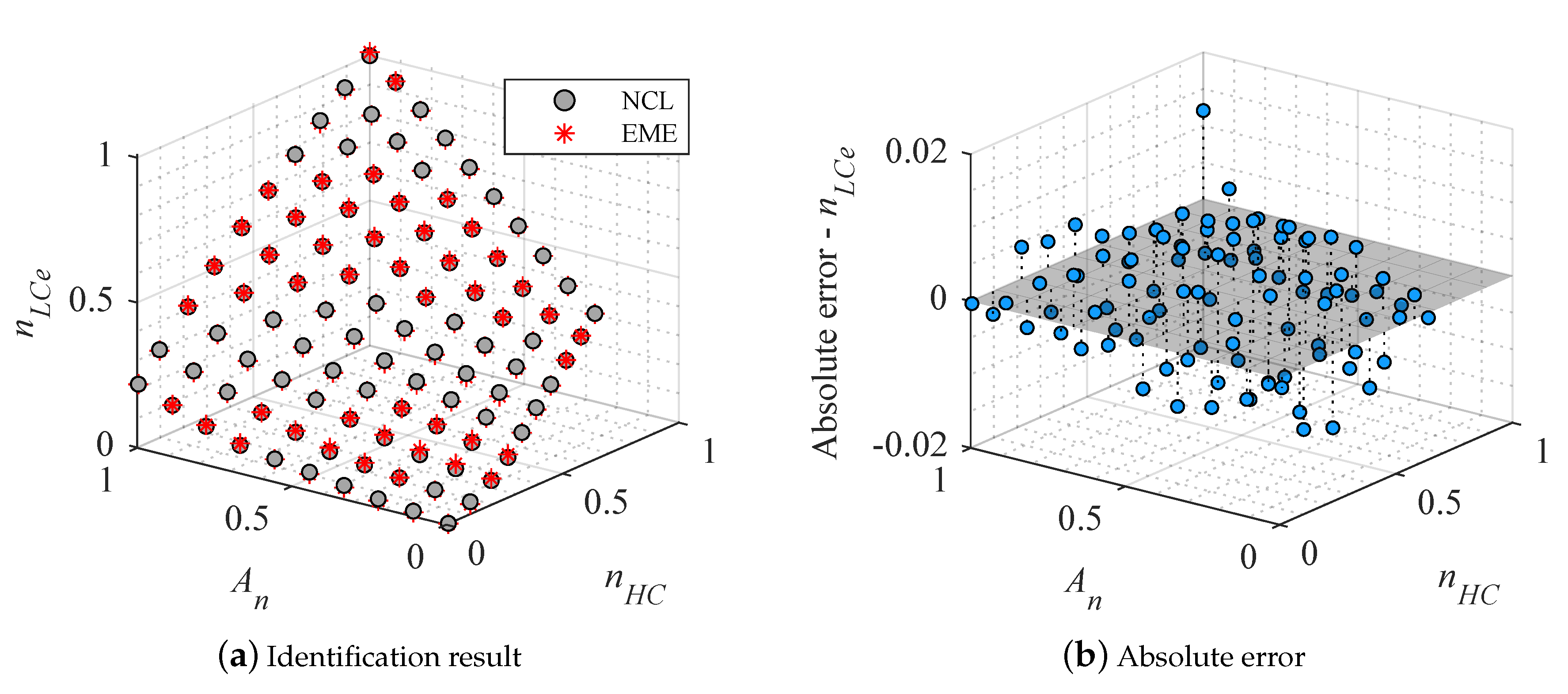
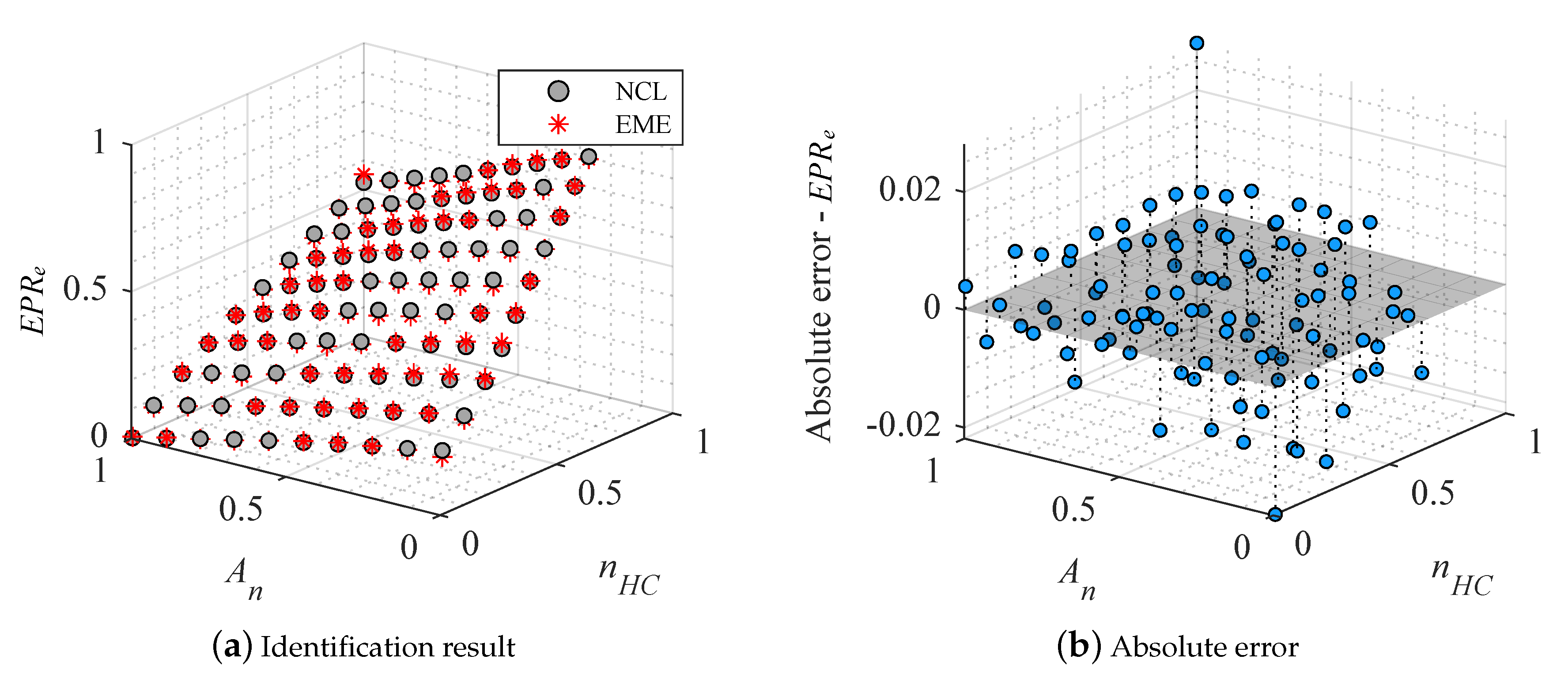
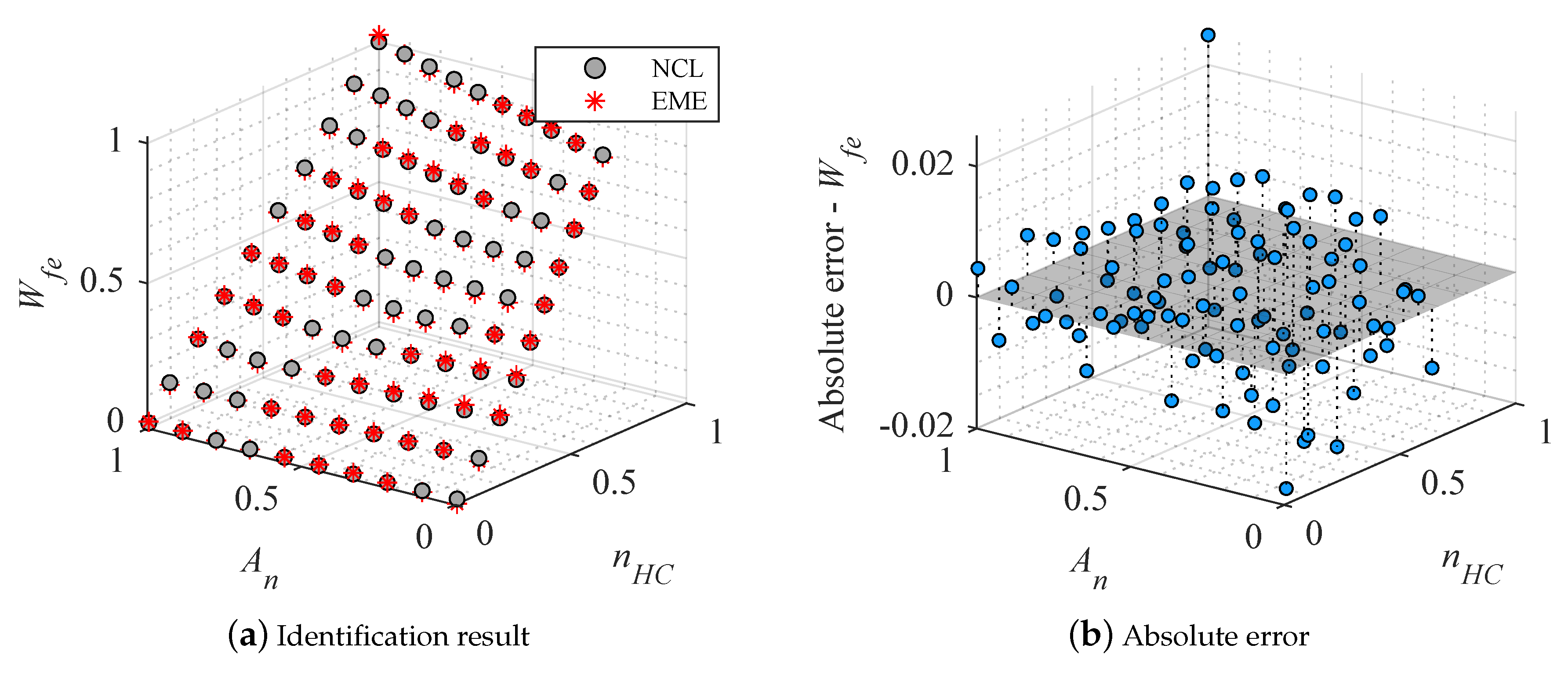
When and are selected as scheduling variables , the EM of the turbofan engine are , , and , which have the structure of Equation (12). The one-to-one correspondence between the input variables and the performance parameters of the turbofan engine is shown as the black circular mark in Figure 2, Figure 3 and Figure 4. These data are obtained by simulating the turbofan engine NCL model carried out in Section 3.1. Therefore, and are taken as independent variables to extract all steady-state results from simulations, and the corresponding dependent variables , , and are obtained. By using the least square method and selecting the 4-order polynomial , the identification results of EM for the turbofan engine are shown in Table 2. Meanwhile, the comparison steady-state results and error analysis are shown in Figure 5, Figure 6 and Figure 7.
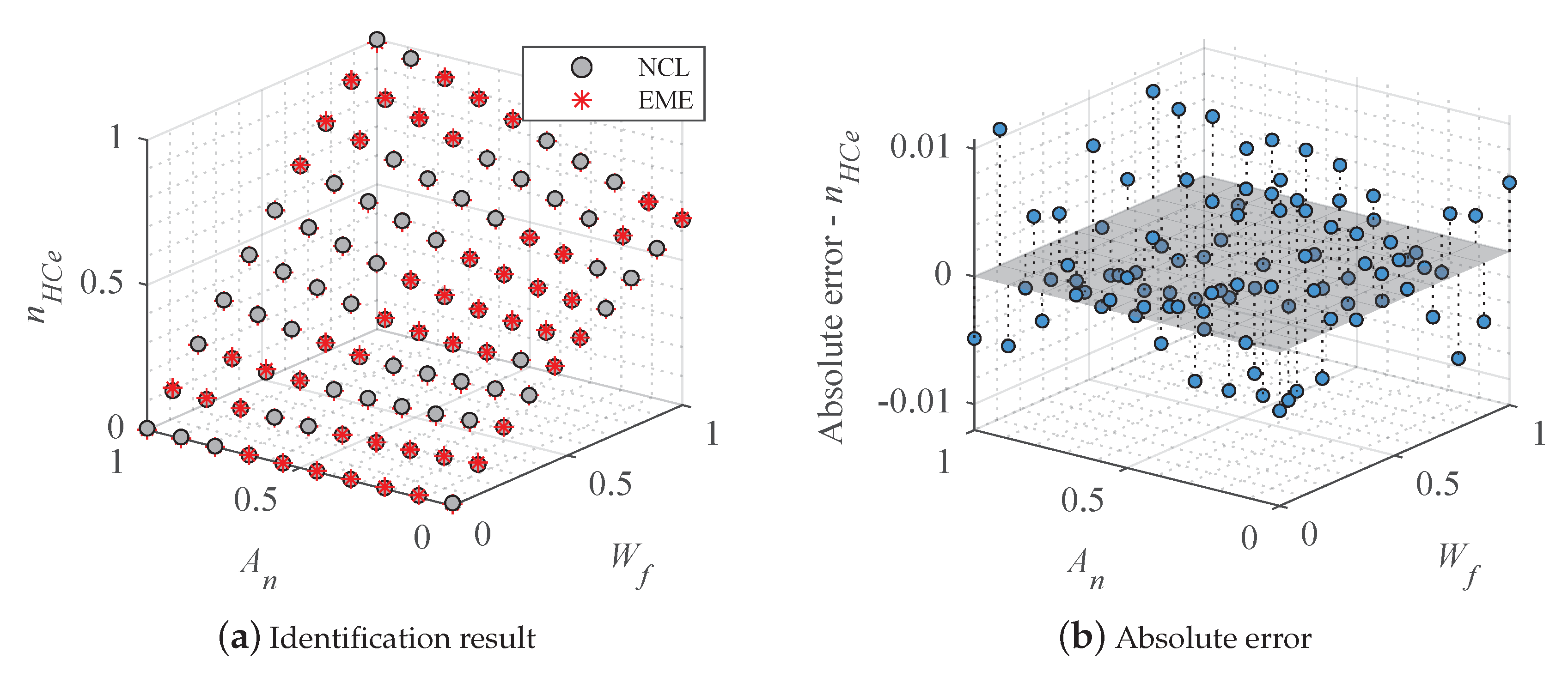
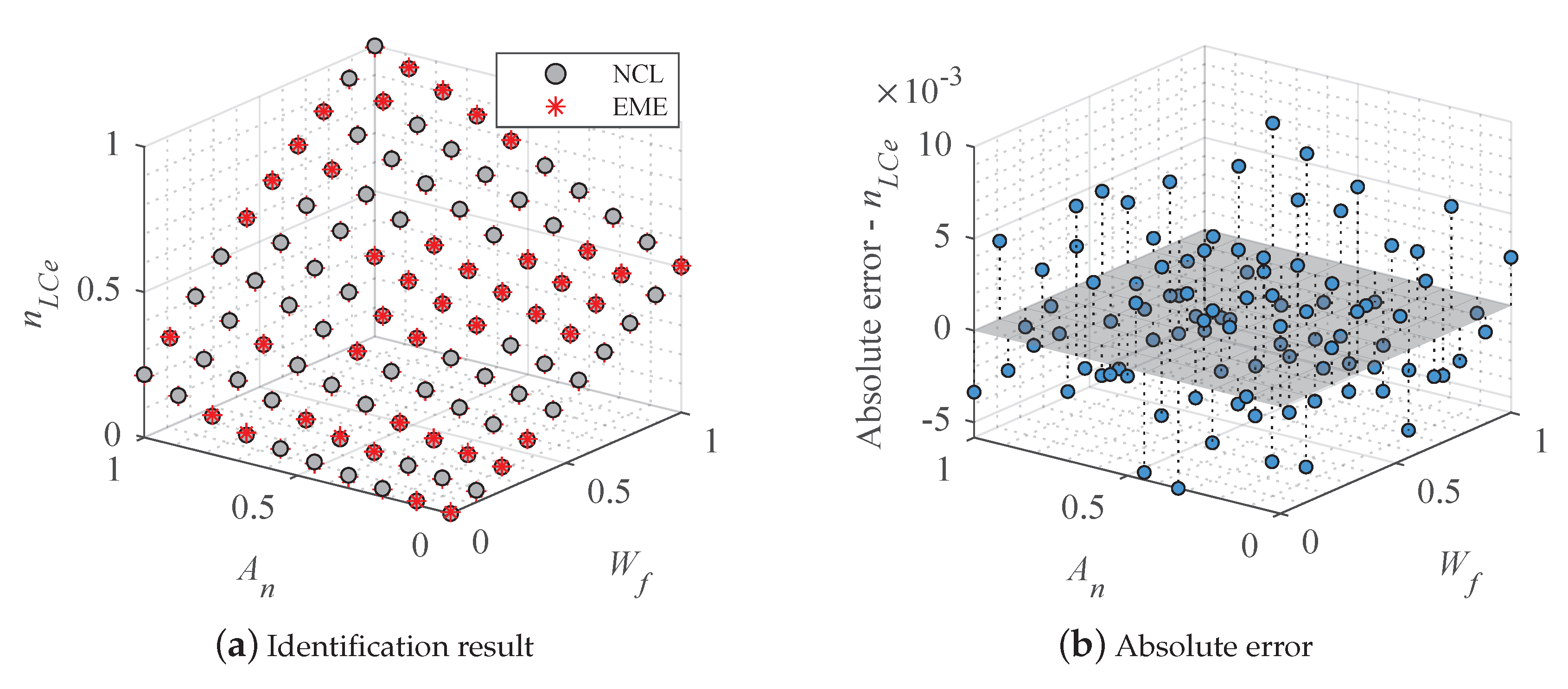
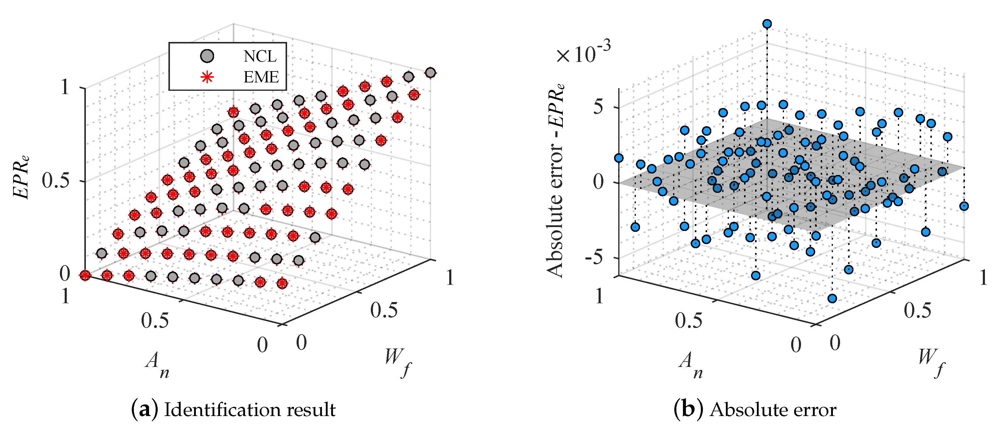
In Figure 5a, Figure 6a, and Figure 7a, the identification results of EM are presented. Among them, the black points are the steady-state results of the NCL model, and the red asterisks are the fitting result. Meanwhile, the absolute errors of the EM with the NCL model’s steady-state results are given in sub-figure (b). Firstly, Figure 5 indicates that the absolute error range of is about −0.015–0.017. In the region composed of (0–0.4) and (0–0.5), the fluctuation of the is caused by the strong nonlinearity of the engine, and the error changes from −0.0084 ( = 0.1034, = 0) to 0.0168 ( = 0.1885, = 0.1111) and then to −0.0132 ( = 0.3761, = 0.1111). The same phenomenon also occurs when and become larger, but the fluctuation amplitude is smaller. Secondly, the absolute error range of is about −0.022–0.028, and the maximum value is 0.028 ( = 1, = 1) in Figure 6. There appears the same strong nonlinear region, in which the error of changes by a wide margin from −0.0219 ( = 0.009, = 0) to 0.0196 ( = 0.1885, = 0.1111) and then to −0.0207 ( = 0.3761, = 0.1111). Thirdly, Figure 7 shows the absolute error of . Its range is about −0.02–0.024, and the maximum one is 0.0246 ( = 1, = 1). Besides, the absolute error of changes from −0.0176 ( = 0.009, =0) to 0.0180 ( = 0.1885, = 0.1111) and then to −0.0188 ( = 0.3814, = 0.2222) in the same strong nonlinear region. Overall, the identification result of the is better than the , and , which is less than 0.017.
The fourth-order polynomial used in this section meets requirement of the accuracy. Usually, when a low order polynomial is used to fit the EM of the system with strong nonlinearity, the steady-state accuracy may not be satisfied. It is considered that increasing order of polynomial is a method to improve the fitting accuracy of the EM. However, the EM with a high-order polynomial also brings problems, such as overfitting and complex expression forms, when the result of the EM is close to the data from the NCL model. It is not conducive to the application of the EME model. In addition, the future research can also adopt switching method and neural network to solve the accuracy problem of the EM.
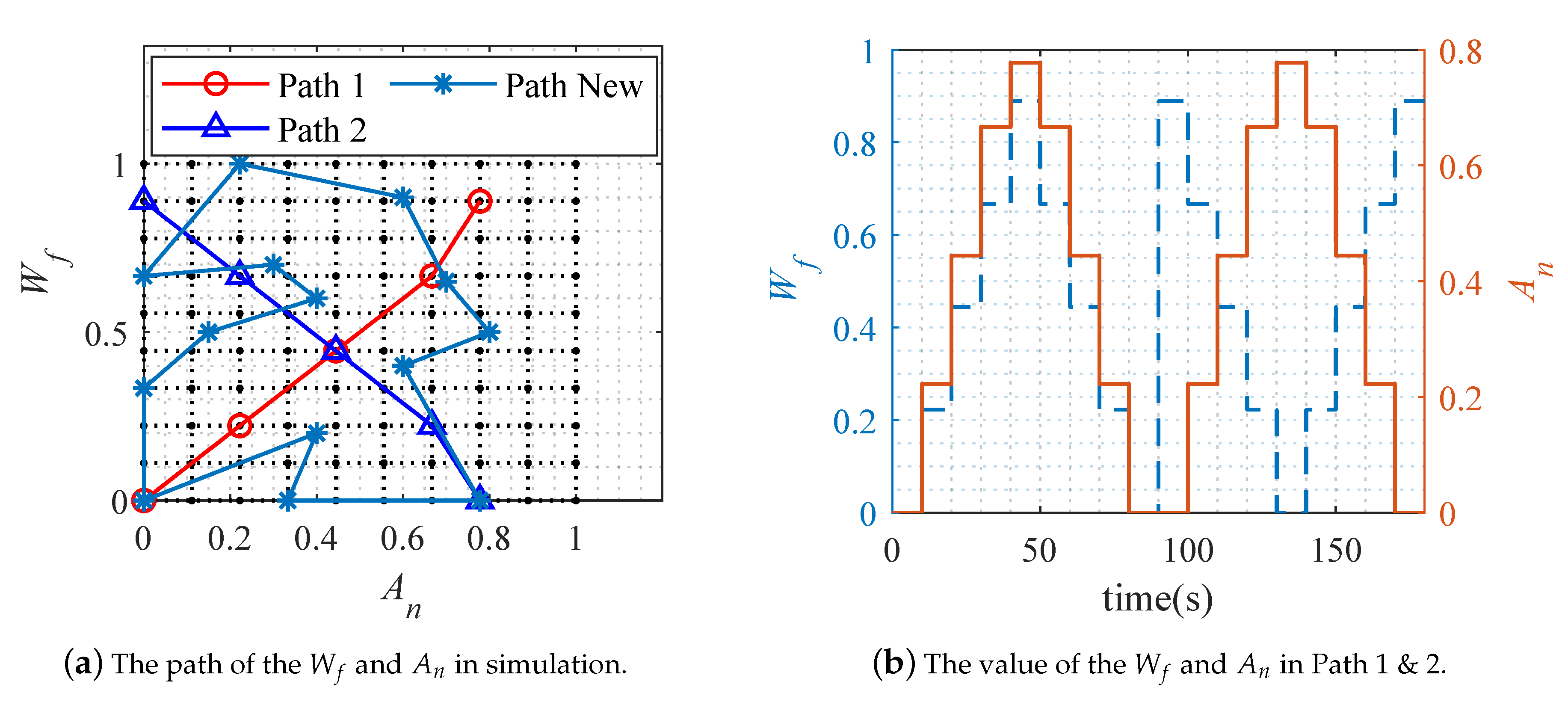
Secondly, the dynamic and static two-step identification method is applied to fit the EME model. After obtaining the steady-state EM, the coefficient matrix , , , and in Equation (11) is identified by the dynamic simulation results of the turbofan engine NCL model. In the simulation of the NCL model, the input variables and that contain two paths considering the sufficient excitation conditions for the identification are shown in Figure 8. As described above, the identification results of the EM require a large number of steady-state data to ensure the accuracy. However, this is not the case for the dynamic parameters of the EME model. If a large number of dynamic processes are adopted or the variation interval of input parameters is excessively reduced in the identification, the results of EME model may be unstable. Therefore, some simulation paths are provided in Figure 8a to obtain the data needed for the dynamic coefficients of the EME model. Path 1 and Path 2 are the diagonal lines of the feasible region of the engine input, and they contain a certain degree of dynamic characteristics. However, neither Path 1 nor Path 2 alone can identify stable dynamic parameters of the EME model. This situation is alleviated after combining Path 1 and Path 2 (Path 1 & 2). At the same time, through the well-designed dynamic parameter identification Path New, better identification results are obtained. Table 3 shows the accuracy results of EME model under different dynamic paths in this paper. Analysis indicators include the sum of squares due to error (), root mean squared error (), and coefficient of determination (). The closer the and are to 0, the better the model selection and fitting, and the more successful the data prediction. The closer is to 1, the better the model fits the data. The results show that the path for dynamic parameters fitting will affect the accuracy of the EME model. Path New has higher accuracy than Path 1 & 2. Facing different engines, a well-designed dynamic path can improve the accuracy of the EME model. The difficulty is that the dynamic path selection is random, and the optimal path for different engines is also difficult to obtain. On the contrary, the combination of Path 1 and Path 2 is the general operating range of turbofan engines. From the results of Table 3, the EME model identified by Path 1 & 2 has the satisfactory accuracy. Therefore, the study adopts Path 1 & 2 to carry out dynamic parameter identification of EME model, and carries out follow-up work based on this path.
Figure 8b shows the input variables changing along Path 1 (0–90 s) and Path 2 (90–180 s). Thus, the scheduling variables , derivatives (), and deviations (, ) in the EME model of the turbofan engine can be obtained. That is, , , , and in Equation (11) can be calculated by the NCL and EM simulations. The coefficient matrix of the EME model is identified as follows:
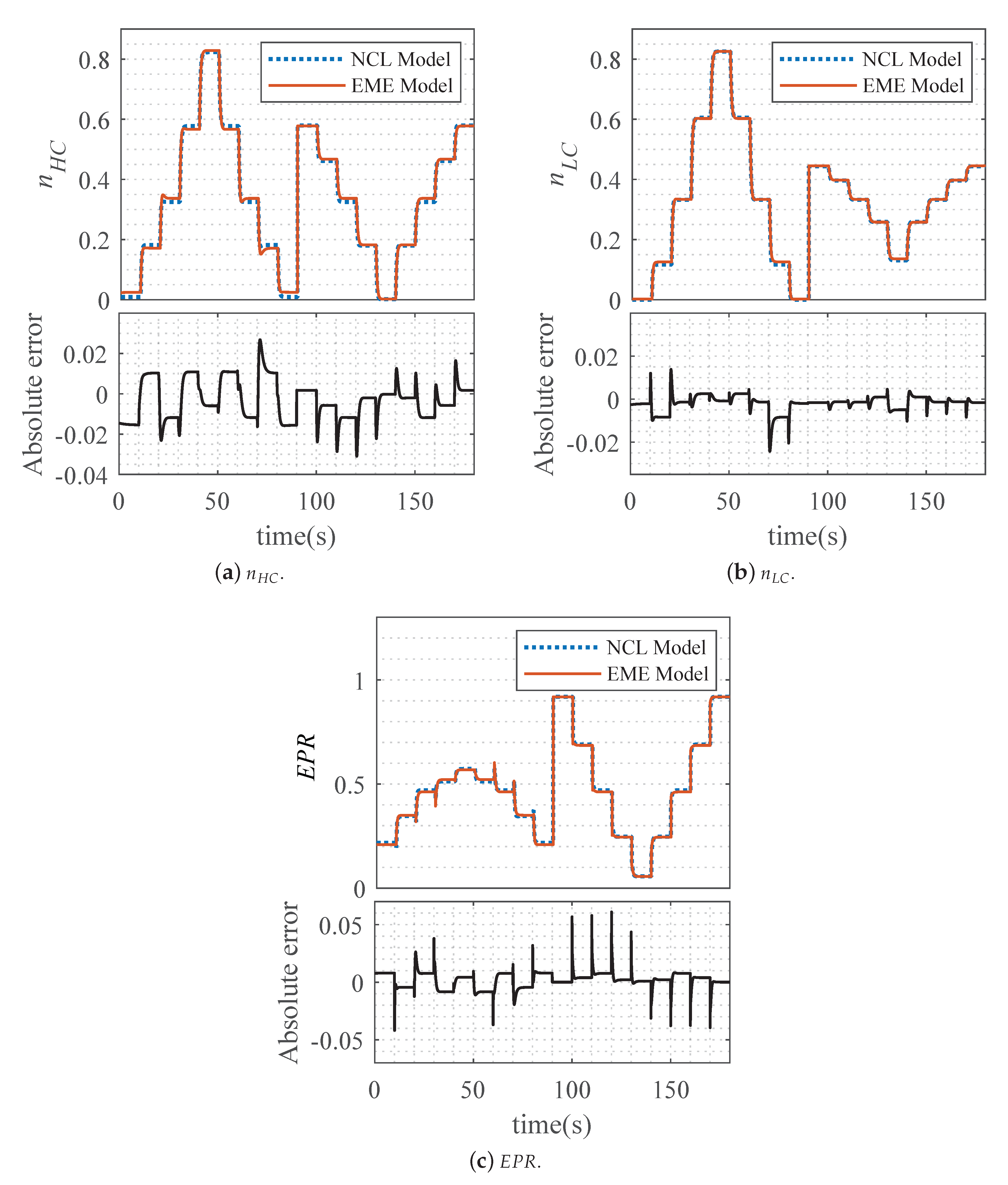
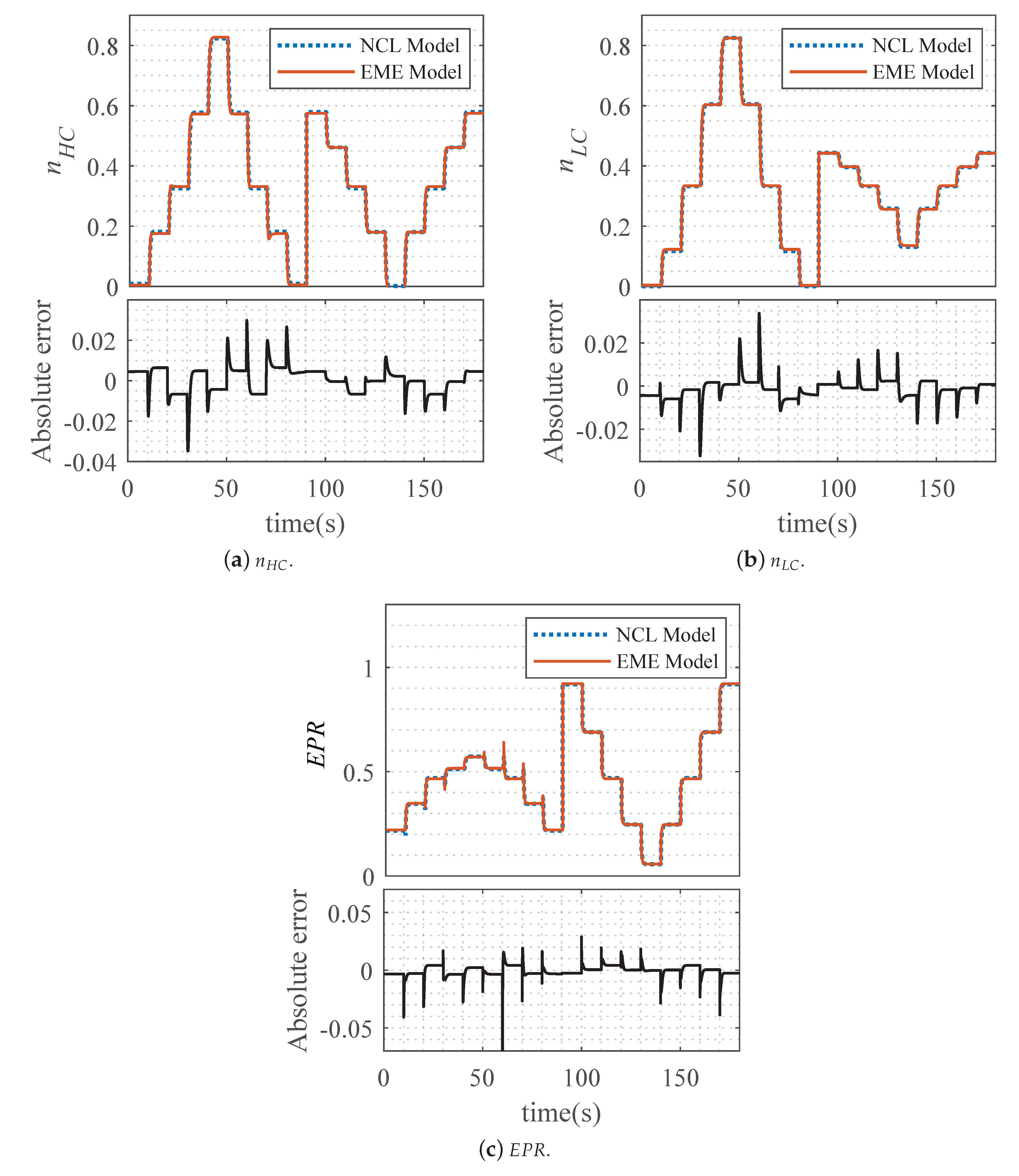
So far, all the parameters of the EME model have been identified. Naturally, it is necessary to validate the accuracy of the EME model. During the verification, the input variables and are still shown in Figure 8. In addition, the comparison and error analysis of the turbofan engine’s NCL model and EME model are shown in Figure 9. The results given by Figure 9 show that the and of the EME () have high steady-state accuracy, while the has low steady-state accuracy. Obviously, the steady-state accuracy of and is determined by the identification results of and , respectively. Meanwhile, the simulations also indicate that the and meet high dynamic accuracy, in which the dynamic time of the EME model is similar to that of the NCL model. In particular, there appears a dynamic error with absolute value around 0.02 for the simulations of at 10 s and 70 s in Figure 9b. In Figure 9c, the results of show a dynamic error with absolute value around 0.05. The large dynamic error of the may be caused by the negative regulation characteristics. However, the shown in Figure 9a is not satisfactory. In the simulation, large overshoot occurs in the EME model at 20 s, 60 s, and 70 s, and the overshoot at 70 s is close to 0.02.
3.3. Effects of Scheduling Variables on Model Accuracy
In Section 3.2, there are some errors in the steady-state and dynamic accuracy of EME () model, especially in . Thankfully, the previous studies have shown that the optimal identification form of the EME model always exists in the nonlinear plants with analytic representation. Although MIMO turbofan engine with strong nonlinearity cannot be expressed analytically, the accuracy of the EME model can also be improved by selecting different combinations of the scheduling variables.
and are selected as to complete the EME model of the turbofan engine in this section. Thus, the form of can be rewritten as follows:
According to Equation (10), , and . Thus, the EME model of the turbofan engine shown in Equation (9) can be replaced by:
Firstly, we identify the EM of the turbofan engine. When and are selected as scheduling variables , the EMs of the turbofan engine are , , and which meet the form of Equation (12). Based on the method given in Section 3.2, the identification results of steady-state EM are shown in Table 5. Meanwhile, the steady-state results and the absolute error analysis of EM with NCL model are shown in Figure 10, Figure 11 and Figure 12. The identification results of EM () are presented in Figure 10a, Figure 11a, and Figure 12a. Among them, the black points are the steady-state results of the NCL model in Section 3.1, and the red asterisks are fitting results. The absolute error of the EM with the NCL model’s steady-state results is given in Figure 10b, Figure 11b, and Figure 12b.
Clearly, the operating range of the is shown in Figure 10, and the maximum absolute error is −0.0120 . However, the strong nonlinear region of the EM in EME () is not significant in EME (). Figure 11 shows that the absolute error range of is about −0.006–0.010. The extremum of the absolute errors are −0.0058 () and 0.0098 () in Figure 11b. In addition, Figure 12b indicates that the absolute error range of is about −0.0060–0.0060. The extremum of the absolute errors are −0.0061 () and 0.0040 () in Figure 12b. In general, the accuracy of the EM in EME () is higher than in EME ().
Secondly, the coefficient matrix , , and in Equation (11) is identified by the dynamic simulation results of the turbofan engine NCL model. Clearly, the specific fitting method is given in Section 3.2. That is, , , , and in Equation (15) can be calculated by the results of the NCL model and the EM. The coefficients of the EME model can be identified as follows:
Because the validation is an important part of modeling, so the validation of the EME model is carried out as follows. The input variables and vary according to the rule shown in Figure 8. Through the simulation, the comparison and error analysis of the turbofan engine’s NCL model and EME model are shown in Figure 13. The results demonstrate the accuracy of the EME model along the design Path 1 & 2.
Figure 13 indicates that , , and in EME () all have high steady-state accuracy, which is determined by the identification results of the EM. Simultaneously, the results also have high dynamic accuracy in EME (). There are large dynamic errors for , , and at 60s, and the values are 0.025, 0.0275, and −0.055, respectively. The EME () model can reflect the overshoot characteristics of in the range of 0–0.035. Besides, the overshoot is less than the EME () at 60 s in Figure 13a. The accuracy of the EME model is affected by , which is confirmed in the simulation. The analysis indicators in Table 3 shows that the EME () model has higher steady-state accuracy than the EME () model, and the identification result of the is more satisfactory. However, direct measurement of inputs, such as real engine fuel, will limit the feasibility of inputs as scheduling variables for the EME model.
3.4. Effects of Noise on Model Accuracy
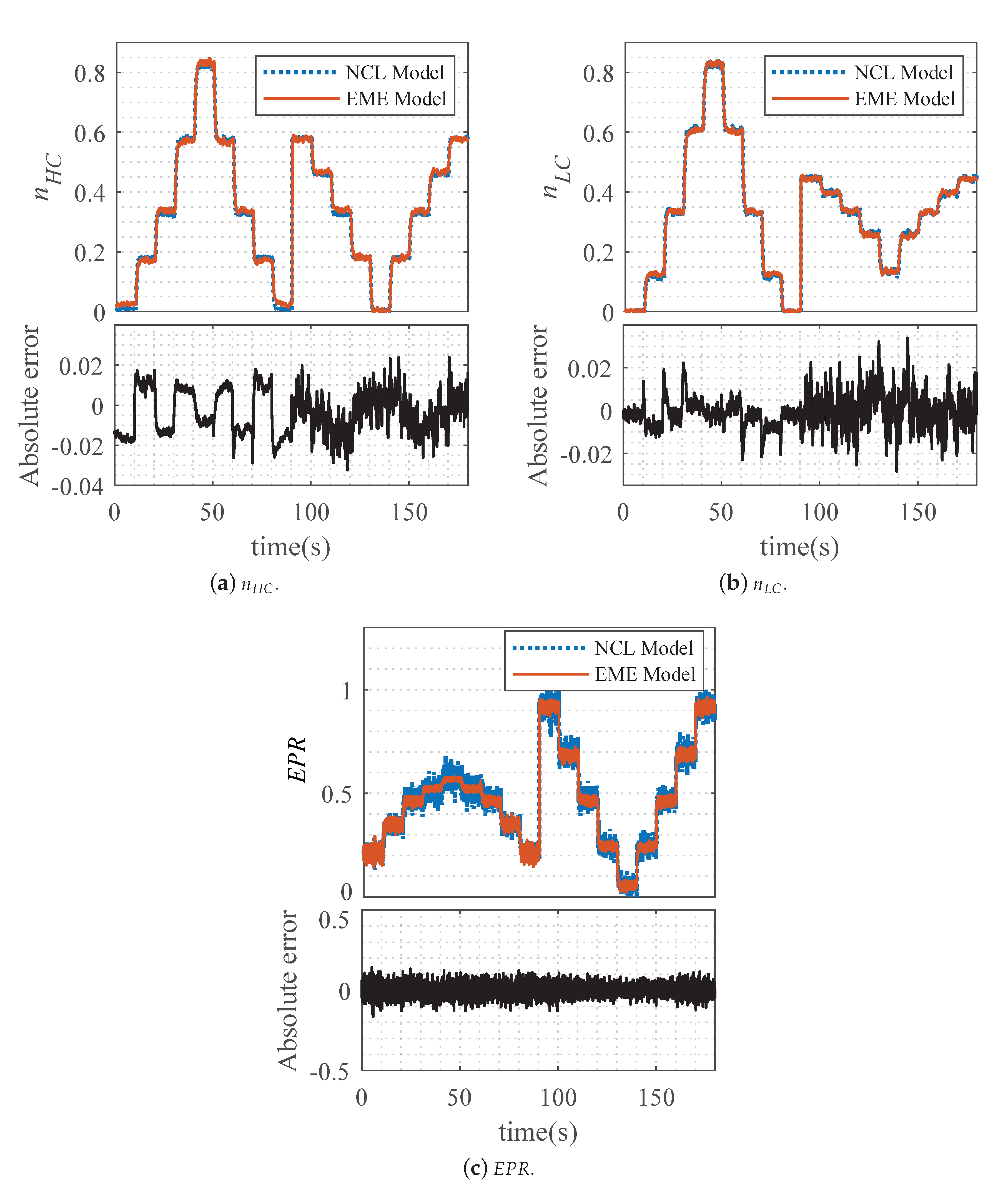
The EME model is a turbofan engine mathematical model based on data identification. These data can be obtained by dynamic simulation of the NCL model, on the one hand, and can be obtained by a large number of real engine tests, on the other hand. However, the cost of engine testing is too high to be used as a data source for the study of EME modeling methods. In fact, there is a big difference between NCL model simulation data and engine test data, among which noise is an important influencing factor. To analyze the influence of noise on EME model identification, we add random noise to the input and of the dynamic Path 1 & 2 in Section 3.2, and complete the EME model identification according to the same process. The output results of the NCL model and the EME model are shown in Table 3.
First, it can be seen from Figure 14 that the input noise has a greater impact on the engine pressure ratio than two rotors and . Secondly, under the effect of input noise, the EME model still has a strong model fitting ability. From the perspective of steady-state results, the EME model can ensure stability; meanwhile, the steady-state accuracy of and is kept about within 2%. Although the pressure ratio error is relatively large, the EME model ensures the steady-state accuracy of the engine and shows a certain filtering ability.
4. Validation and Stability Analysis of the EME Model
4.1. Validation at Dynamic Off-Design Conditions
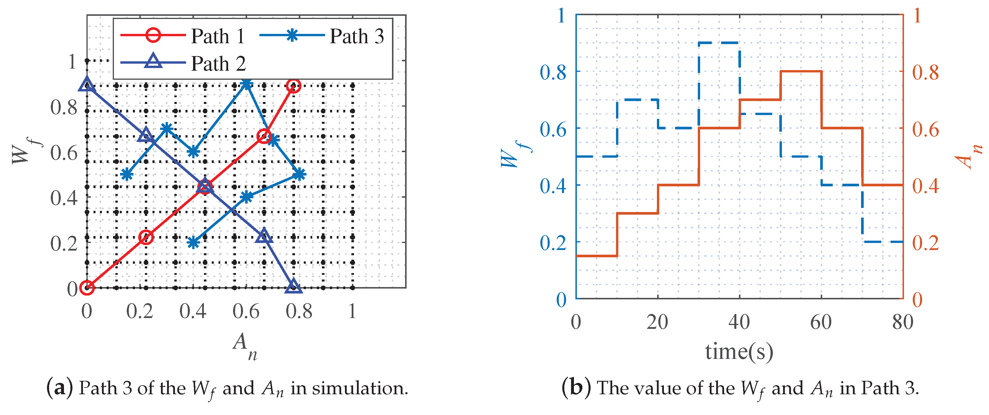
This paper proposes that the dynamic coefficients of the EME model are identified by Path 1 & 2 shown in Figure 15a. Despite differences in accuracy, the identification results of the EME model shown in Section 3.2 and Section 3.3 are satisfactory in control-oriented modeling. However, verifying the accuracy of the EME model on the design path alone is insufficient. Therefore, this section considers the validation of the EME () model and the EME () model at dynamic off-design conditions. Path 3, which is different from Path 1 and Path 2, is given in Figure 15a. Figure 15b shows the corresponding input variables for the validation.
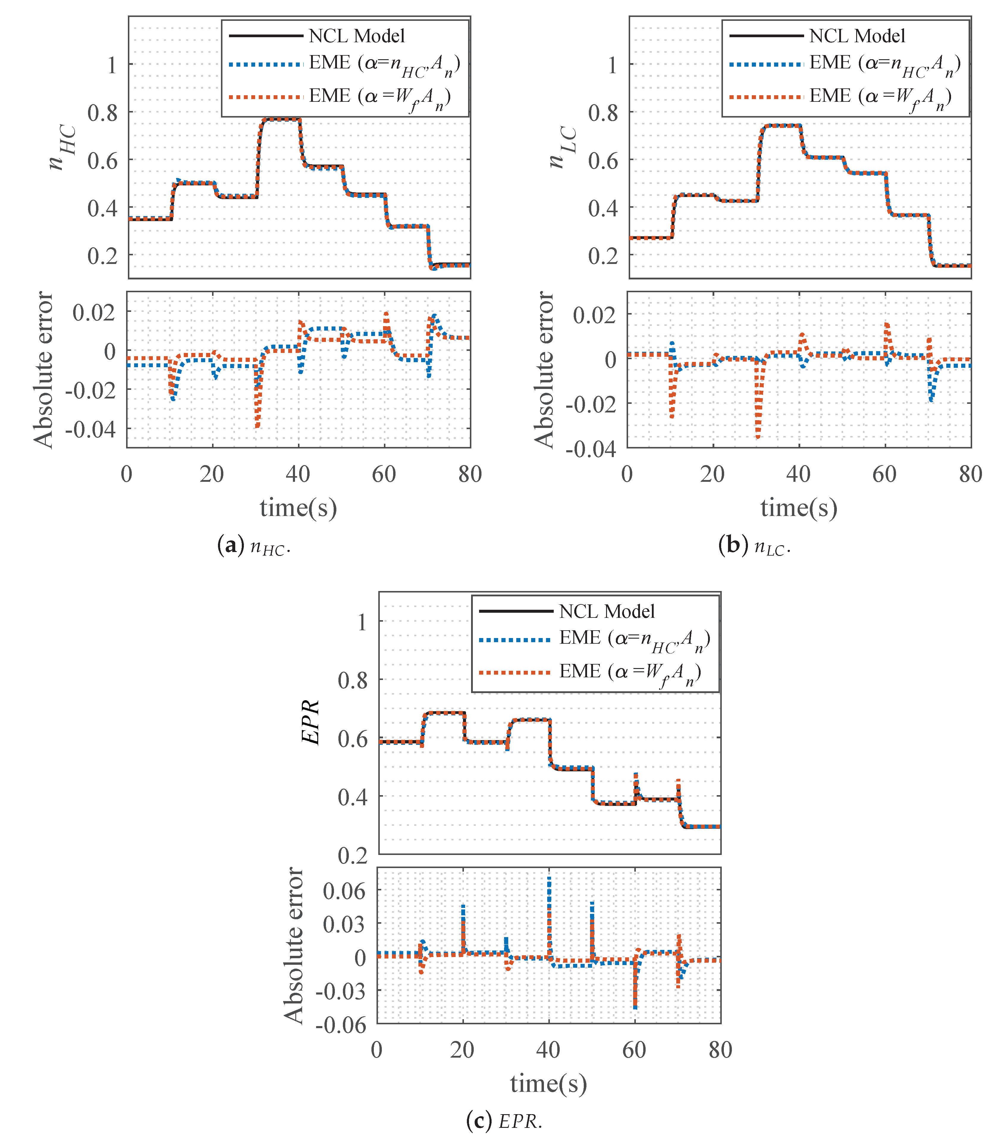
The input variables given in Figure 15b are used in the NCL, EME (), and EME () model of the turbofan engine for simulation. The output variables , and of the turbofan engine are shown in Figure 16. At the same off-design conditions, the validation results of different turbofan engine models, and the absolute errors between the EME () model to the NCL model and the EME () model to the NCL model are shown in Figure 16.
Firstly, the steady-state , and of the EME model with different scheduling variables have different accuracy. In particular, Figure 16a shows that there is a difference between the EME () and EME () model in the steady-state accuracy of . The EME () model has higher steady-state accuracy at the off-design conditions given in Path 3, which is consistent with the results obtained from Path 1 and 2. In addition, Figure 16b indicates that the steady-state accuracy of at off-design conditions is almost the same, except that the steady-state accuracy of the EME () is lower than the EME () at 70–80 s. The steady-state accuracy of at off-design conditions is similar to that shown in Figure 16c, except that the EME () has lower steady-state accuracy than the EME () at 40–50 s. Secondly, Figure 16 shows that the dynamic time of the EME () and EME () is almost the same, which means that the two EME models can well meet the dynamic process of the turbofan engine. Meanwhile, Figure 16a indicates that there is an overshoot of at 30 s, which is caused by the strong nonlinearity of the engine.
In short, the EME model has satisfactory accuracy at both design and off-design conditions. The model meets the demand of real-time simulation. These are significant for the control-oriented model of the turbofan engine. Although it is difficult to find the EME model with the smallest error for the strongly nonlinear system including turbofan engines that cannot be expressed analytically, we can identify the EME model that meet the requirements of the accuracy by selecting different combinations of the scheduling variables.
4.2. Linearization and Stability Analysis
As a control-oriented model of the MIMO turbofan engine, it is significant for the EME model to meet the requirements of the control system design. At present, the most common and well-developed control methods are linear control, while the nonlinear control methods have difficulties in solving and practical applications. Moreover, many nonlinear control methods involve the linearization of the complex nonlinear plants. Therefore, a wide-range linear model with high accuracy can greatly reduce the difficulty of a control system design for nonlinear plants. Nevertheless, the EME model is a nonlinear parameter-varying system, and some coefficients of the linearization for the EME model are missing in , , , and due to the selection of the scheduling variables. , , , , , and are missing in Equation (11), whereas , , , , , and are missing in Equation (15). Thus, it is important to obtain a complete linearization result of the EME model. Fortunately, Property 2 of the EME model introduced in Section 2.2 can be used to complete the linearization results, which contains the constraints of the EME model. For Equation (11), the sufficient and necessary conditions Equation (6) given in Property 2 can be expanded to:
Considering the orthogonal properties of the scheduling variables, we have:
Substituting Equation (18) into Equation (17), the missing coefficients in Equation (11) can be completed as:
Similarly, the missing coefficients in Equation (15) can be completed as:
Obviously, after the EME () model is complemented by Equation (19) and the EME () model is complemented by Equation (20), the linear model of the MIMO turbofan engine at any steady-state operating point can be obtained. As the turbofan engine is a stable system which can be seen from the simulation in Section 3.1, the EME model should be stable, and it is verified in the time domain simulation shown in Figure 9 and Figure 13. However, the analysis from the time domain is not rigorous enough. Stability analysis is necessary for the linearized results of the EME model.
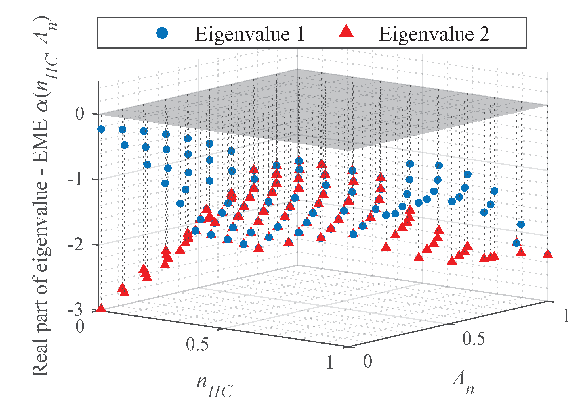
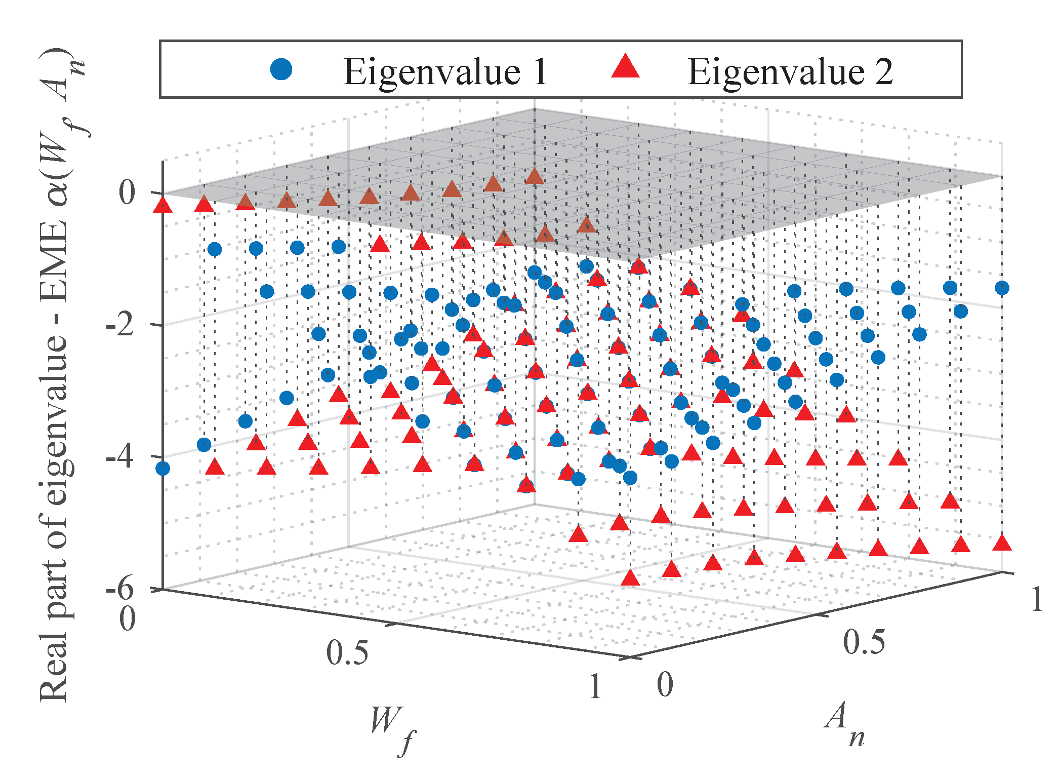
The sufficient and necessary condition for the stability of linear systems is that all the roots of the characteristic equations of closed-loop systems have negative real parts. This condition means all the matrix from the linearization results of the EME model with the state space form have negative real parts. Thus, the linearization of the EME () model and the EME () model are completed at the 100 steady-state points given in Figure 2, Figure 3 and Figure 4, and the real part of the eigenvalues of matrix is shown in Figure 17 and Figure 18.
Since all the eigenvalues of have negative real parts, the linearization results of the EME models () are stable within the range of the scheduling variables. So far, the accuracy and stability of the EME model are proved by the time domain simulation and linearization results, which indicates that the EME model can be used as real-time simulation model for control system design.
5. Conclusions
This paper investigates a control-oriented model of nonlinear MIMO turbofan engines using the equilibrium manifold method. To obtain the EME model of turbofan engine with input variables and and output variables , , and , extending the equilibrium manifold modeling method from the SISO system to the MIMO system is studied. The main conclusions of this article are:
- The two EME models that contain the input variables () and the output variables () are established. The results of the steady state EM () show that the absolute error range of (−0.015–0.017) is better than (−0.022–0.028) and (−0.02–0.024). The absolute error range of EM () are about −0.006–0.010 in , −0.0060–0.0060 in , and −0.012–0.010 in . Obviously, the accuracy of EME () is higher than EME (). Because of the simple structure, the EME model also meets the needs of real-time simulation. Meanwhile, the EME model still shows high accuracy under the influence of noise.
- The EME model meets the accuracy requirement of the simulation and the stability in the entire range of operating conditions. The validity of the EME model is verified by simulation at off-design points. At the same time, the results also show that the identification of the dynamic coefficients for the EME model can be completed through only considering simple paths. Depending on the property of the EME model, the linearization of the model is completed. By calculating the eigenvalues, both EME models (,) have stable linearization result, thus ensuring that the EME model can be regarded as a control-oriented model.
Furthermore, the dynamic coefficients of the EME model have low dependence of the excitation condition in identification. It means that the identification of the dynamic coefficients needs few data, which is different from the general method of model identification. This finding provides a possibility for the EME model to solve the performance degradation of the turbofan engine in future.
Author Contributions
Conceptualization, C.L., Z.W., J.C. and D.Y.; methodology, C.L., Z.W., J.C. and D.Y.; software, C.L.; validation, C.L. and Z.W.; formal analysis, J.C. and D.Y.; investigation, C.L. and Z.W.; resources, J.C. and D.Y.; writing—original draft preparation, C.L., Z.W. and J.C.; writing—review and editing, L.D., H.L. and D.Y.; project administration, C.L. and Z.W.; funding acquisition, J.C. and D.Y. All authors have read and agreed to the published version of the manuscript.
Funding
This research work is supported by the National Science and Technology Major Project (2017-V-0004-0054).
Institutional Review Board Statement
Not applicable.
Informed Consent Statement
Not applicable.
Data Availability Statement
Not applicable.
Conflicts of Interest
The authors declare no conflict of interest.
References
- Dong, Z.; Li, D.; Wang, Z.; Sun, M. A review on exergy analysis of aerospace power systems. Acta Astronaut. 2018, 152, 486–495. [Google Scholar] [CrossRef]
- Liu, J.; Ma, Y.; Zhu, L.; Zhao, H.; Liu, H.; Yu, D. Improved gain scheduling control and its application to aero-engine LPV synthesis. Energies 2020, 13, 5967. [Google Scholar] [CrossRef]
- Aretakis, N.; Roumeliotis, I.; Alexiou, A.; Romesis, C.; Mathioudakis, K. Turbofan engine health assessment from flight data. J. Eng. Gas. Turbines Power Trans. ASME 2015, 137, 041203. [Google Scholar] [CrossRef]
- Zhou, S.; Ma, H.; Yang, Y.; Zhou, C. Investigation on propagation characteristics of rotating detonation wave in a radial-flow turbine engine combustor model. Acta Astronaut. 2019, 160, 15–24. [Google Scholar] [CrossRef]
- Zheng, J.L.; Chang, J.T.; Ma, J.C.; Yu, D.R. Performance uncertainty propagation analysis for control-oriented model of a turbine-based combined cycle engine. Acta Astronaut. 2018, 153, 39–49. [Google Scholar] [CrossRef]
- Link, C.J.; Jack, D.M. Aircraft Engine Controls: Design, System Analysis and Health Monitoring; AIAA Education Series; American Institute of Aeronautics and Astronautics: Reston, VA, USA, 2009. [Google Scholar]
- Szuch, J.R.; Seldne, K. Real-Time Simulation of F100-PW-100 Turbofan Engine Using the Hybrid Computer; NASA TMX-3261; National Aeronautics and Space Administration: Washington, DC, USA, 1975. [Google Scholar]
- Ballin, M.G. A High Fidelity Real-Time Simulation of a Small Turboshaft Engine; NASA-TM-100991; National Aeronautics and Space Administration: Washington, DC, USA, 1988. [Google Scholar]
- Ma, J.X.; Chang, J.T.; Ma, J.C.; Bao, W.; Yu, D.R. Mathematical modeling and characteristic analysis for over-under turbine based combined cycle engine. Acta Astronaut. 2018, 148, 141–152. [Google Scholar] [CrossRef]
- Frederick, D.K.; Decastro, J.A.; Litt, J.S. User’s Guide for the Commercial Modular Aero-Propulsion System Simulation (C-MAPSS); NASA/TM-215026; National Aeronautics and Space Administration: Washington, DC, USA, 2007. [Google Scholar]
- Csank, J.; May, R.D.; Litt, J.; Jonathan, L.; Ten-Huei, G. Commercial Modular Aero-Propulsion System Simulation 40k (C-MAPSS40k) User’s Guide; NASA/TM-216831; National Aeronautics and Space Administration: Washington, DC, USA, 2010. [Google Scholar]
- Evans, C.; Rees, D.; Hill, D. Frequency-domain identification of gas turbine dynamics. IEEE Trans. Control Syst. Technol. 1998, 6, 651–662. [Google Scholar] [CrossRef]
- Sugiyama, N. Derivation of ABCD System Matrices from Nonlinear Dynamic Simulation of Jet Engines; AIAA 92-3319; American Institute of Aeronautics and Astronautics: Washington, DC, USA, 2012. [Google Scholar]
- Feng, Z.P.; Sun, J.; Huang, J. A new method for establishing a state variable model of aeroengine. J. Aerosp. Power 1998, 13, 435–438. [Google Scholar]
- Leibov, R. Aircraft turbofan engine linear model with uncertain eigenvalues. IEEE Trans. Autom. Control 2002, 47, 1367–1369. [Google Scholar] [CrossRef]
- Rugh, W.J.; Shamma, J.S. Research on gain scheduling. Automatica 2000, 36, 1401–1425. [Google Scholar] [CrossRef]
- Leith, D.J.; Leithead, W.E. Survey of gain-scheduling analysis and design. Int. J. Control 2000, 73, 1001–1025. [Google Scholar] [CrossRef]
- Wolodkin, G.; Balas, G.J.; Garrard, W.J. Application of parameter-dependent robust control synthesis to turbofan engines. J. Guid. Control Dyn. 1999, 22, 833–838. [Google Scholar] [CrossRef]
- Shamma, J.S.; Cloutier, J.R. Gain-scheduled missile autopilot design using linear parameter varying transformations. J. Guid. Control Dyn. 2012, 16, 256–263. [Google Scholar] [CrossRef]
- Bhattacharya, R.; Balas, G.J.; Kaya, M.A.; Packard, A. Nonlinear receding horizon control of an F-16 aircraft. J. Guid. Control Dyn. 2002, 25, 924–931. [Google Scholar] [CrossRef] [Green Version]
- Huang, J.Y.; Ji, G.L.; Zhu, Y.C. Identification of multi-model LPV models with two scheduling variables. J. Process Control. 2012, 22, 1198–1208. [Google Scholar] [CrossRef]
- Rotondo, D.; Nejjari, F.; Puig, V. Quasi-LPV modeling, identification and control of a twin rotor MIMO system. Control Eng. Pract. 2013, 21, 829–846. [Google Scholar] [CrossRef]
- Lu, F.; Huang, J.N.Q.J.J.Q.; Qiu, X.J. In-flight adaptive modeling using polynomial LPV approach for turbofan engine dynamic behavior. Aerosp. Sci. Technol. 2017, 64, 223–236. [Google Scholar] [CrossRef]
- Liu, T.J.; Sun, D.X.X.M.; Richter, H.; Zhu, F. Robust tracking control of aero-engine rotor speed based on switched LPV model. Aerosp. Sci. Technol. 2019, 91, 382–390. [Google Scholar] [CrossRef]
- Yu, D.R.; Cui, T.; Bao, W. Equilibrium manifold linearization model for normal shock position control systems. J. Aircr. 2005, 42, 1344–1347. [Google Scholar]
- Sui, Y.F.; Yu, D. Identification of expansion model based on equilibrium manifold of turbojet engine. Hangkong Xuebao/Acta Aeronaut. Astronaut. Sin. 2007, 28, 531–534. [Google Scholar]
- Yu, D.R.; Zhao, H.; Xu, Z.; Sui, Y.F.; Liu, J.F. An approximate non-linear model for aeroengine control. Proc. Inst. Mech. Eng. Part G J. Aerosp. Eng. 2011, 225, 1366–1381. [Google Scholar] [CrossRef]
- Zhao, H.; Liu, J.F.; Yu, D.R. Approximate nonlinear modeling and feedback linearization control for aeroengines. J. Eng. Gas Turbines Power Trans. ASME 2001, 133, 111601. [Google Scholar] [CrossRef]
- Liu, X.F.; Yuan, Y. Nonlinear system modeling and application based on system equilibrium manifold and expansion model. J. Comput. Nonlinear Dyn. 2014, 9, 021013. [Google Scholar] [CrossRef]
- Liu, X.F.; Zhao, L. Approximate nonlinear modeling of aircraft engine surge margin based on equilibrium manifold expansion. Chin. J. Aeronaut. 2012, 25, 663–674. [Google Scholar] [CrossRef] [Green Version]
- Shi, Y.; Zhao, J.; Liu, Y.Y. Switching control for aero-engines based on switched equilibrium manifold expansion model. IEEE Trans. Ind. Electron. 2016, 64, 3156–3165. [Google Scholar] [CrossRef]
- Chen, C.; Zhao, J. Switching control of acceleration and safety protection for turbofan aero-engines based on equilibrium manifold expansion model. Asian J. Control. 2018, 20, 1689–1700. [Google Scholar] [CrossRef]
- Zhou, W.X. Research on Object-Oriented Modeling and Simulation for Aeroengine and Control System; Nanjing University of Aeronautics and Astronautics: Nanjing, China, 2007. [Google Scholar]
- Fei, X.; Huang, J.Q.; Zhou, W.X. Modeling of and simulation research on turbofan engine based on MATLAB/SIMULINK. J. Aerosp. Power 2007, 22, 2134–2138. [Google Scholar]
- Pan, M.; Huang, H.; Huang, J.Q. T-S fuzzy modeling for aircraft engines: The clustering and identification approach. Energies 2019, 12, 3284. [Google Scholar] [CrossRef] [Green Version]
- Zhou, X.; Lu, F.; Huang, J.Q. Fault diagnosis based on measurement reconstruction of hpt exit pressure for turbofan engine. Chin. J. Aeronaut. 2019, 32, 1156–1170. [Google Scholar] [CrossRef]
- Xu, W.; Huang, J.Q.; Qin, J.K.; Pan, M.X. Limit protection design in turbofan engine acceleration control based on scheduling command governor. Chin. J. Aeronaut. 2021, 34, 67–80. [Google Scholar] [CrossRef]
- Pan, M.; Zhang, K.; Chen, Y.; Huang, J.Q. A new robust tracking control design for turbofan engines: H∞/leitmann approach. Appl. Sci. 2017, 7, 439. [Google Scholar] [CrossRef] [Green Version]
Figure 1.
The input variables and for the simulation of the NCL model.

Figure 2.
The simulation results of under ten simulation conditions.

Figure 3.
The simulation results of under ten simulation conditions.

Figure 4.
The simulation results of under ten simulation conditions.

Figure 5.
The identification result and absolute error of the EM .

Figure 6.
The identification result and absolute error of the EM .

Figure 7.
The identification result and absolute error of the EM .

Figure 8.
The input variables and for the identification of the EME model.

Figure 9.
The identification result and absolute error of the EME () model.

Figure 10.
The identification result and absolute error of the EM .

Figure 11.
The identification result and absolute error of the EM .

Figure 12.
The identification result and absolute error of the EM .

Figure 13.
The identification result and absolute error of the EME () model.

Figure 14.
The validation of the EME () model with noise conditions in Path 1 & 2.

Figure 15.
The input variables and for the identification of the EME model at dynamic off-design conditions.
Figure 15.
The input variables and for the identification of the EME model at dynamic off-design conditions.

Figure 16.
The validation of the EME (,) model at dynamic off-design conditions.

Figure 17.
The real part of eigenvalue of for the EME () model.

Figure 18.
The real part of eigenvalue of for the EME () model.


Table 1.
Subscript corresponding to different EM.
| n | |
|---|---|
| h | |
| l | |
| f | |
| s | |
| p |
Table 2.
The coefficients of the EM .
| Coef 1 | Result 1 | Coef 2 | Result 2 | Coef 3 | Result 3 |
|---|---|---|---|---|---|
| −0.0031 | −0.0278 | 0.1875 | |||
| 0.0952 | 0.1859 | 0.0355 | |||
| 0.0029 | −0.4295 | −0.5316 | |||
| 0.1822 | 0.4005 | 0.4544 | |||
| −0.0662 | −0.1310 | −0.1465 | |||
| 0.1586 | 1.0829 | 0.8436 | |||
| 1.1210 | 0.4523 | 0.2797 | |||
| −0.2957 | −0.2919 | −0.0796 | |||
| −0.0700 | −0.1283 | −0.2328 | |||
| 2.0277 | 1.6503 | 1.6111 | |||
| −2.0877 | −2.8265 | −3.1073 | |||
| 0.2379 | 0.8793 | 0.9245 | |||
| −1.9790 | −1.5050 | −1.6747 | |||
| 1.1385 | 1.4396 | 1.7264 | |||
| 0.5497 | 0.2737 | 0.2624 | |||
Table 3.
Accuracy results of EME model under different dynamic paths.
| Path | Output | ||||
|---|---|---|---|---|---|
| 1&2 | 0.9508 | 0.0103 | 0.9979 | ||
| 0.1539 | 0.0041 | 0.9996 | |||
| 0.4772 | 0.0073 | 0.9990 | |||
| New | 0.2701 | 0.0035 | 0.9994 | ||
| 0.1623 | 0.0042 | 0.9996 | |||
| 0.1615 | 0.0042 | 0.9997 | |||
| 1&2 with noise | 0.9204 | 0.0101 | 0.9980 | ||
| 0.1912 | 0.0046 | 0.9995 | |||
| 0.5516 | 0.0078 | 0.9988 | |||
| 1&2 | 0.3830 | 0.0065 | 0.9992 | ||
| 0.2505 | 0.0053 | 0.9994 | |||
| 0.1983 | 0.0047 | 0.9996 |
Table 4.
The coefficients of the EME model.
| Coef 1 | Result 1 | Coef 2 | Result 2 | Coef 3 | Result 3 |
|---|---|---|---|---|---|
| −0.2362 | −1.4657 | −0.0875 | |||
| 1.5140 | 0.2270 | −0.0401 | |||
| −2.1259 | −2.0621 | −0.9159 | |||
| 0.0148 | −0.1033 | 0.0749 | |||
| 0.0023 | −0.0175 | −0.0227 | |||
| 1.7453 | 1.3592 | 0.3058 | |||
Table 5.
The coefficients of the EM .
| Coef 1 | Result 1 | Coef 2 | Result 2 | Coef 3 | Result 3 |
|---|---|---|---|---|---|
| 0.0047 | 0.0044 | 0.2207 | |||
| 0.0261 | 0.0832 | −0.2133 | |||
| −0.0989 | −0.0001 | 0.0389 | |||
| 0.0896 | 0.1935 | −0.0500 | |||
| −0.0207 | −0.0678 | 0.0054 | |||
| 1.0655 | 0.2134 | 0.6443 | |||
| −1.0625 | 0.2511 | 0.5970 | |||
| 1.2794 | 0.6322 | −0.7356 | |||
| −0.3306 | −0.2856 | 0.1915 | |||
| −1.1696 | 0.8536 | 0.5171 | |||
| 1.9950 | 0.0144 | −1.2565 | |||
| −0.7915 | −0.4243 | 0.5088 | |||
| 1.0608 | −0.9268 | −0.5161 | |||
| −0.7422 | 0.0930 | 0.4477 | |||
| −0.3170 | 0.3604 | 0.1315 | |||
Table 6.
The coefficients of the EME model.
| Coef 1 | Result 1 | Coef 2 | Result 2 | Coef 3 | Result 3 |
|---|---|---|---|---|---|
| 0.5015 | 3.7503 | −0.5078 | |||
| −0.0845 | 1.0956 | −0.1344 | |||
| −2.2704 | −1.4782 | 0.3204 | |||
| 0.6230 | −4.2386 | 0.0782 | |||
| 2.2073 | 0.9056 | −0.7508 | |||
| −2.6501 | −2.0944 | 0.9199 | |||
Publisher’s Note: MDPI stays neutral with regard to jurisdictional claims in published maps and institutional affiliations. |
© 2021 by the authors. Licensee MDPI, Basel, Switzerland. This article is an open access article distributed under the terms and conditions of the Creative Commons Attribution (CC BY) license (https://creativecommons.org/licenses/by/4.0/).
Share and Cite
MDPI and ACS Style
Lv, C.; Wang, Z.; Dai, L.; Liu, H.; Chang, J.; Yu, D. Control-Oriented Modeling for Nonlinear MIMO Turbofan Engine Based on Equilibrium Manifold Expansion Model. Energies 2021, 14, 6277. https://doi.org/10.3390/en14196277
AMA Style
Lv C, Wang Z, Dai L, Liu H, Chang J, Yu D. Control-Oriented Modeling for Nonlinear MIMO Turbofan Engine Based on Equilibrium Manifold Expansion Model. Energies. 2021; 14(19):6277. https://doi.org/10.3390/en14196277
Chicago/Turabian StyleLv, Chengkun, Ziao Wang, Lei Dai, Hao Liu, Juntao Chang, and Daren Yu. 2021. "Control-Oriented Modeling for Nonlinear MIMO Turbofan Engine Based on Equilibrium Manifold Expansion Model" Energies 14, no. 19: 6277. https://doi.org/10.3390/en14196277
Note that from the first issue of 2016, this journal uses article numbers instead of page numbers. See further details here.