Article

Capsule Vehicle Dynamics Based on Levitation Coil Design Using Equivalent Model of a Sidewall Electrodynamic Suspension System

1
Department of Transportation System Engineering, Korea Railroad Research Institute Campus, University of Science and Technology, Uiwang-si 16105, Gyeonggi-do, Korea
2
New Transportation Innovation Research Centre, Korea Railroad Research Institute, Uiwang-si 16105, Gyeonggi-do, Korea
*
Author to whom correspondence should be addressed.
Energies 2021, 14(16), 4979; https://doi.org/10.3390/en14164979
Submission received: 9 July 2021 / Revised: 10 August 2021 / Accepted: 10 August 2021 / Published: 13 August 2021

Abstract

:
A levitation system based on sidewall electrodynamic suspension (EDS) is considered for a capsule vehicle, which is a next-generation high-speed transportation system currently being studied. This levitation system does not require controlling of the gap between the guideway and the vehicle on which the superconducting electromagnet is mounted. However, when the vehicle is operated in a levitated state, the ride comfort is worse than that of the levitation system based on electromagnetic suspension (EMS), making it necessary to develop methods that can ensure good riding comfort. In addition, because the EDS system is complex and nonlinear with a combination of electromagnetics and mechanical dynamics, it is complicated to analyze the dynamic characteristics of the capsule vehicle, and the corresponding numerical analysis is time-consuming. Therefore, to easily understand the running dynamics of a capsule vehicle in the sidewall EMS system, the magnetic suspension characteristics corresponding to the primary suspension are simply modeled by considering the levitation stiffness in the vertical direction and the guidance stiffness in the lateral direction, similar to that in the case of the mechanical suspension. In this study, mathematical models of the levitation and guidance stiffnesses with respect to the speed and position of a vehicle body running at high speeds in a levitated state in the sidewall EDS system were derived for three design proposals of the levitation coil. The dynamic behavior of the vehicle based on the three design proposals was investigated by simulating a capsule vehicle model with 15 degrees of freedom.

1. Introduction

One of the recently developed transportation systems is the capsule train system [1,2,3]. This system has a capsule vehicle equipped with a superconducting magnet that enables it to move in a tube at an ultra-high speed of 1000 km/h. There are two types of magnetic levitation systems [4,5,6]: electromagnetic suspension (EMS) [7,8] and electrodynamic suspension (EDS) [9,10,11]. As shown in Figure 1a, in the case of EMS, the electromagnet of the vehicle is located under the magnetic material of the guideway and generates a levitation force through the attraction between the two. The guidance force is generated through the magnetic material and an electromagnet attached to the side of the guideway and the bogie. EDS is illustrated in Figure 1b; when the vehicle with electromagnets attached to the bottom or side drives along the guideway with a levitation coil installed over a certain speed, levitation force and guidance force are generated through the repulsive force. Unlike the EMS system, which requires gap control between the running body and the guideway, the EDS system does not require any gap control. In addition, because the EMS method is unsuitable for driving speeds of over 500 km/h, the EDS system is more popular for capsule train systems [12,13,14,15].
When the EDS system is applied to maglev, which is a high-speed magnetic levitation system employed in Japan, the characteristics of the magnetic stiffness corresponding to the primary suspension between the running vehicle and the guideway should be identified as accurately as possible [16,17,18,19,20,21,22,23,24]. The characteristics of the magnetic stiffness are used to understand the running dynamics of the capsule vehicle in advance to provide excellent ride comfort to passengers. In particular, because the EDS system is a complex nonlinear system that combines electromagnetics and mechanical dynamics, it is complicated to analyze the dynamic characteristics of the capsule vehicle, and the corresponding numerical analysis is time-consuming. Therefore, to easily understand the running dynamics of a capsule vehicle in the sidewall electrodynamic suspension system, the magnetic suspension characteristics corresponding to the primary suspension are simply modeled by considering the levitation stiffness in the vertical direction and the guidance stiffness in the lateral direction, similar to that in the case of the mechanical suspension.
In this study, the running dynamics of a capsule vehicle were studied by reflecting the levitation and guidance stiffnesses of the capsule vehicle system. Nonlinear mathematical equations for the levitation and guidance stiffnesses were established using the levitation and guidance forces of the traveling body designed in a reduced form [20,21] before designing a real-size capsule vehicle. The equations were then expanded and modified to be applicable to a real-size capsule vehicle. These equations were applied to the equation of motion of the capsule vehicle modeled with 15 degrees of freedom to study the dynamic characteristics of the capsule vehicle. To date, only the dynamic characteristics of the EDS magnetic levitation system for the maximum traveling speed of 450 km/h have been reviewed [21]. By contrast, in this paper, the dynamic characteristics from low to high speed (300 km/h, 600 km/h, and 900 km/h) are considered. Furthermore, whereas the results of examining the levitation stiffness and guide stiffness were previously published for only one levitation coil, in this study, simulations were performed on three types of levitation coils and the results compared to determine the most suitable levitation coil design for the capsule vehicle system.

2. Electromagnetic Force between Superconducting Electromagnet and Levitation Coil

This section presents the electromagnetic force acting on the traveling body (hereinafter referred to as “traveling body”) designed in a reduced form before designing the full-size capsule vehicle. The levitation system applied to the capsule vehicle system comprises a superconducting electromagnet mounted on a running vehicle and a levitation coil installed on the guideway. As shown in Figure 2, the arrangement of the superconducting electromagnet and the levitation coil is the same on both sides of the running vehicle [12,13,14]. The levitation coil is installed at regular intervals on both sides of the guideway. The high-speed vehicle travels below the reference position (z = 0) at a certain height in the vertical direction. Owing to the characteristics of the EDS method, the vertical and lateral vibrations are expected to be high [17,18,19].
Figure 3 shows the levitation coil considered in this study, and two coils are connected up and down to form the shape of “8.” In addition, as listed in Table 1, three levitation coil design models (or design proposals) were considered [14], and the magnetomotive force in each case was equal to 300 kAt.
Figure 4 shows the results obtained using the finite element analysis of the magnetic force distributed in the space between the superconducting magnet and the levitation coil [14]. The force applied to the traveling body varies significantly with the position of the body [22,23,24].

3. Force Applied to the Traveling Body at the Force Balance Position

The running dynamics of a traveling body of mass M are obtained by applying the levitation and guidance forces to the equations of motion such as Equations (1) and (2). F y is the guidance force, F z is the levitation force, and g is the gravitational acceleration.
M d 2 y d t 2 = F y
M d 2 y d t 2 = F z M g
The characteristics of the force applied to the traveling body are identified under the following assumptions.
(a)
The center of mass of the vehicle is considered as the origin of the coordinate axis of the vehicle, and the levitation and guidance forces applied to the vehicle by the superconducting electromagnet act on the pole of the superconducting electromagnet.
(b)
The traveling body travels at a constant speed v in the running direction (x direction).
The weight of the traveling body frame is 450 kg and that of the superconducting electromagnet is also 450 kg [12]. Considering that the traveling body weighs 1350 kg, including two superconducting electromagnets, the force due to its own weight is 1350 kg × 9.8 m/s2 = 13,230 (N). Table 2 shows the two vertical positions where the levitation force approximating 13,230 N is generated for each design. From Table 2, the position where the total weight of the traveling body and the levitation force is balanced is approximately 0.05 m below the center of the levitation coil for Design A and approximately 0.04 m for Designs B and C. When a magnetomotive force of 300 kAt is applied to the high-speed traveling body at a constant speed of 500 km/h, the levitation and guidance forces generated at the position where the total weight of the traveling body and the levitation force are balanced in the vertical direction and at a distance of 0.02 m in the lateral direction are shown in Figure 5 for Design A.
Both the levitation and guidance forces include a nonzero constant component and a sinusoidal component. The part corresponding to the sine wave is related to the pitch ( τ l ) of the levitation coil. In other words, this period is the time required for the superconducting electromagnet to pass through the levitation coil and is calculated using Equation (3). The period T is 1.944 msec for Design A, 2.916 msec for Design B, and 3.888 msec for Design C.
T = τ l v
Table 3 shows the average value and fluctuation in the levitation and guidance forces for each design. From Table 3, Design A has the highest force and Design C the lowest. In addition, the magnitude of the guidance force is the highest in Design A and the lowest in Design C. The change rate of the guidance force is the lowest in Design B.
On the other hand, the levitation and guidance forces depend on the speed of the traveling body, vertical position, and lateral position, and there is a fluctuation component with respect to the levitation coil pitch [22,23,24,25,26]. In addition, in the EDS system, the levitation and guidance forces between the traveling body and the guideway (or levitation coil) can be expressed in the form of an equivalent stiffness, similar to that in the case of the primary suspension of a railway vehicle [21,25,26]. In other words, the equivalent stiffness due to the levitation force (hereinafter referred to as “levitation stiffness”) can be considered the primary vertical spring of the railway vehicle, and the equivalent stiffness (hereinafter referred to as “guidance stiffness”) because of the guidance force can be considered the primary lateral spring of the railway vehicles. At this time, the levitation stiffness and guidance stiffnesses have nonlinearities owing to the characteristics of the EDS system. Considering this point, the levitation and guidance forces can be expressed as in Equations (4) and (5), respectively.
k z ( v , x , y , z ) = F y / z
k y ( v , x , y , z ) = F z / y
where k z and k y are the levitation and guidance stiffnesses, respectively; F z and F y are the levitation and guidance forces, respectively; and v is the running speed of the traveling body.

4. Equivalent Model of Levitation Stiffness

As mentioned previously, the levitation and guidance forces depend on the speed of the traveling body, the vertical position, and the lateral position. Moreover, because they include a fluctuation component with respect to the levitation coil pitch, these characteristics should be reflected in the levitation and guidance stiffnesses.

4.1. Levitation Stiffness with Respect to the Speed of the Traveling Body

Figure 6 shows the relationship between the levitation force and the speed of the traveling body when the traveling body passes the levitation coil at a position where the load of the traveling body is balanced with the levitation force for Designs A, B, and C. In Designs A, B, and C, the levitation force tends to converge as the speed increases. In addition, as the speed decreases, the levitation force is low, and the traveling body runs considerably below the center position of the levitation coil. Therefore, the traveling body will not be levitated below a certain speed and will be driven by the wheels. Generally, in an RL circuit forming the levitation coil, the time constant is L/R, and because this levitation system is an RL circuit, the attenuation of the current can be approximated as e t   R / L [21]. Since the current in the RL circuit is similar to the speed in the mechanical system, the levitation and guidance stiffness can be expressed as an exponential function of the speed.
Figure 7 shows the levitation stiffness with respect to the speed for each design as a graph using Equation (4). The levitation stiffness was calculated based on the position where the load of the traveling body and levitation force were balanced (Design A: z = −0.05 m, Designs B and C: z = −0.04 m).
From this result, the levitation stiffness can be approximated as a function of the speed, as expressed in Equation (6). The values of the parameters in Equation (6) are given in Table 4 [27,28,29]. Here, the unit of k z z is kN/m.
k z z = a z e ( b z / v )          

4.2. Levitation Stiffness with Respect to the Vertical Position

Figure 8 shows the relationship between the levitation stiffness and the vertical position of the traveling body by speed for each design. Figure 8 shows only the average value, ignoring the fluctuation component due to the pitch of the levitation coil. The levitation stiffness has a nonlinear relationship with the vertical position of the traveling body.
Figure 9 shows the levitation stiffness with respect to the vertical position for each design when the speed of the traveling body is v = 500 km/h, including fluctuations due to the pitch of the levitation coil. Because the levitation force varies depending on the pitch of the levitation coil, the average, maximum, and minimum values are displayed together. As shown in Figure 6, the fluctuation in this levitation force is almost sinusoidal, and this component can also be expressed as an approximate equation.
From Figure 9, the maximum, average, and minimum values of the levitation stiffness with respect to the vertical positions can be expressed as quadratic functions for Designs A, B, and C, as expressed in Equations (7)–(15) [21,25,26,27,28,29]. Here, the unit is N/m.
Design A:
k l , m a x = ( 310.3 × 10 3 1.204 × 10 7 z 2 )
k l , a v g = ( 295.3 × 10 3 1.165 × 10 7 z 2 )
k l , m i n = ( 280.2 × 10 3 1.125 × 10 7 z 2 )
Design B:
k l , m a x = ( 379.1 × 10 3 1.535 × 10 7 z 2 )
k l , a v g = ( 363.7 × 10 3 1.437 × 10 7 z 2 )
k l , m i n = ( 344.8 × 10 3 1.326 × 10 7 z 2 )
Design C:
k l , m a x = ( 377.1 × 10 3 1.409 × 10 7 z 2 )
k l , a v g = ( 369.1 × 10 3 1.377 × 10 7 z 2 )
k l , m i n = ( 355.7 × 10 3 1.331 × 10 7 z 2 )
To understand the running dynamics of the traveling body, the levitation stiffness obtained from the relationship with the speed and vertical position of the traveling body needs to be expressed mathematically. As expressed in Equations (16) and (17), the levitation stiffness can be expressed by dividing the average value ( k z , a v g ) and the oscillating component ( k z , o s c ) generated by the pitch of the levitating coil. In Equations (16) and (17), c 1 ,   c 2 ,   c o 1 ,   and   c o 2   are functions related to the speed and have the form of Ae ( B / v ) as mentioned above, where A and B are coefficients determined by the shape of the levitation coil. Therefore, the coefficients for each design can be obtained from Equations (6) and (7)–(15). Table 5 lists the coefficients for each of the three design models.
k z , a v g ( v , z ) = c 1 ( v ) + c 2 ( v ) z 2
k z , o s c ( v , z ) = c o 1 ( v ) + c o 2 ( v ) z 2
On the other hand, one period of the oscillation component of the levitation stiffness is the time passing through one pitch of the levitation coil, and the levitation stiffness is a function of the position x in the traveling direction and the position z in the vertical direction and can be expressed as Equation (18) [21,25,26]. The pitch ( τ l ) of the levitation coil for each design is listed in Table 5.
k l ( v , x , z ) = k z , a v g ( v , z ) + k z , o s c ( v , z )   sin ( 2 π x / τ l )

4.3. Levitation Stiffness with Respect to the Lateral Position

Finally, to express the levitation stiffness in terms of the lateral position of the traveling body as a mathematical approximation, the characteristics of the levitation stiffness with respect to both the vertical and lateral positions of the traveling body should be determined. Figure 10 shows the average value of the levitation stiffness and oscillation components with respect to the vertical and lateral positions of the body when the traveling speed v = 500 km/h for Design A. They can be expressed as mathematical Equations (19) and (20), respectively.
k l ,   y z = ( 5.4 195.4 z 2 ) ( 54.42 + 1.0 × 10 4 y 2 )
k l ,   y z , o s c = ( 0.629 7.696 z 2 ) ( 2255 + 1.0 × 10 4 y 2 )
Using the same process, the levitation stiffness with respect to the vertical and lateral positions of the traveling body can be obtained for Designs B and C. Notably, the approximate equations derived in this way do not represent the values at the position where the load and levitation force of the traveling body are balanced. Therefore, to match the balance position of the traveling body, we should consider z = −0.05 m for Design A and z = −0.04 m for Designs B and C. Table 6 lists the final equations for the levitation stiffness, which are summarized by reflecting the force balance position and the effects of speed.

5. Equivalent Model of Guidance Stiffness

5.1. Guidance Stiffness with Respect to the Speed of the Traveling Body

Similar to the case of levitation stiffness, the guidance stiffness is also shown in Figure 11 when the guidance stiffness with respect to the speed of the traveling body for each design model is graphically represented by Equation (5). The guidance stiffness was calculated based on the point where y = ±0.02 m in the lateral direction for all three designs.
From this result, the guidance stiffness can be approximated as a function of the speed, as expressed in Equation (21). The values of the parameters of Equation (21) are given in Table 7 [27,28,29]. Here, the unit of k y y is kN/m.
k y y = a y e ( b y / v )

5.2. Guidance Stiffness with Respect to the Lateral Position

Figure 12 shows the relationship between the guidance stiffness and the lateral position of the traveling body by speed for each design. Figure 12 shows only the average value, ignoring the fluctuation component due to the pitch of the levitation coil. The guidance stiffness has a nonlinear relationship with the lateral position of the traveling body.
Figure 13 shows the guidance stiffness with respect to the lateral position for each design when the speed of the traveling body is v = 500 km/h, including fluctuations due to the pitch of the levitation coil. Because the guidance force varies depending on the pitch of the levitation coil, the average, maximum, and minimum values are displayed together. As in the case of the levitation stiffness, the fluctuation in this guidance force is almost sinusoidal, and this component can also be expressed as an approximate equation.
From Figure 13, the maximum, average, and minimum values of the guidance stiffness with respect to the lateral position can be expressed as a quadratic function for Designs A, B, and C, as expressed in Equations (22)–(30) [21,25,26,27,28,29]. Here, the unit is N/m.
Design A:
k g , m a x = ( 220.03 × 10 3 7.056 × 10 6 y 2 )
k g , a v g = ( 181.1 × 10 3 0.450 × 10 6 y 2 )
k g , m i n = ( 140 × 10 3 0.776 × 10 6 y 2 )
Design B:
k g , m a x = ( 139.7 × 10 3 3.903 × 10 6 y 2 )
k g , a v g = ( 136.3 × 10 3 2.756 × 10 6 y 2 )
k g , m i n = ( 132.5 × 10 3 1.079 × 10 6 y 2 )
Design C:
k g , m a x = ( 118.4 × 10 3 3.773 × 10 6 y 2 )
k g , a v g = ( 110.1 × 10 3 3.425 × 10 6 y 2 )
k g , m i n = ( 95.42 × 10 3 3.025 × 10 6 y 2 )
As in the case of the levitation stiffness, the guidance stiffness can be expressed by dividing the average value and the oscillating component generated by the pitch of the levitating coil. In Equations (31) and (32), d 1 ,   d 2 ,   d o 1 ,   and   d o 2   are expressed in the form of an exponential function related to the speed of the traveling body, including the coefficient determined by the shape of the levitation coil in the same way as the levitation stiffness. Table 8 shows the d 1 ,   d 2 ,   d o 1 ,   and   d o 2 values for each design obtained from Equations (21) and (22)–(30). The unit is N/m.
k y , a v g ( v , y ) = d 1 ( v ) + d 2 ( v ) y 2
k y , o s c ( v , y ) = d o 1 ( v ) + d o 2 ( v ) y 2
Considering the relationship between the period of the oscillation component of the guidance stiffness and the pitch of the levitation coil, the guidance stiffness can be expressed as in Equation (33) for the position x in the traveling direction and the lateral position y [21,25,26]. The pitch ( τ l ) of the levitation coil for each design is listed in Table 8.
k g ( v , x , y ) = k y , a v g ( v , y ) + k y , o s c ( v , y )   sin ( 2 π x / τ l )

5.3. Guidance Stiffness with Respect to the Vertical Position

Finally, to express the guidance stiffness with respect to the vertical position of the traveling body as a mathematical approximation, the characteristics of the guidance stiffness with respect to both the vertical and lateral positions of the traveling body should be identified. Figure 14 shows the average value of the guidance stiffness and oscillation components with respect to the vertical and lateral positions of the body when the traveling speed v = 500 km/h for Design A. They can be expressed as mathematical Equations (34) and (35), respectively.
k g , y z = ( 0.279 + 191.9 z 2 ) ( 230.8 + 10 4 y 2 )
k g , y z , o s c = ( 0.24 + 53.64 z 2 ) ( 107.2 + 10 4 y 2 )
Using the same process, the guidance stiffness with respect to the vertical and lateral positions of the traveling body can be obtained for Designs B and C. Notably, the approximate equations derived in this way do not represent the stiffness at the position where the load and levitation force of the traveling body are balanced. Therefore, to match the balance position of the traveling body, z = −0.05 m for Design A and z = −0.04 m for Designs B and C should be considered. Table 9 shows the final equations for the guidance stiffness, which are summarized by reflecting the force balance position and the effect of speed.

6. Comparison of Dynamic Behavior by Model

6.1. Dynamic Model of Capsule Vehicle

As seen in the previous section, the levitation and guidance stiffnesses of the three designs have opposite tendencies. In other words, the levitation stiffness is the lowest for Design A and the highest for Design C, and the guidance stiffness is the lowest for Design C and the highest for Design A. Simulations using MATLAB and Simulink S/W were performed to determine the difference in the dynamic behavior of the capsule vehicle when Designs A, B, and C were applied to the levitation system of the capsule vehicle.
The capsule train used in the simulation comprised two bogies and one body. As shown in Figure 15, eight superconducting electromagnets are mounted on each bogie, four of which are on each of the left and right sides [25,26]. The superconducting electromagnet plays a role in supplying the levitation and guidance forces to the vehicle through action with the levitation coil, which can be expressed as a primary suspension ( k l ,   k g ) in Figure 15. k l and k g are the levitation and guidance stiffnesses, respectively. In addition, two secondary suspensions ( k s v ,   k s l ,   c s v ,   c s l ) are located between the vehicle body and the bogie. The masses of the carbody and bogie are denoted by mc and mb, respectively. Table 10 lists the values of the parameters shown in Figure 15. The guideway irregularity in Figure 16 is the disturbance applied to the bogie [30,31,32].
As shown in Figure 15, the mathematical model of the capsule vehicle was composed of 15 degrees of freedom considering the vertical, lateral, roll, pitch, and yaw directions of the front and rear bogies and the body. In this study, the vertical displacement ( z f b , z r b ) and lateral displacement ( y f b , y r b ) of the carbody and front and rear bogies affecting the running stability of the vehicle were studied. The vertical and lateral accelerations of the carbody affecting the ride comfort were also studied. The equation of motion of the capsule vehicle can be expressed as state Equations (36) and (37) with a state vector x(t), a system matrix A, an input matrix B, and an output matrix C.
{   x ˙ ( t ) = A x ( t ) + B u ( t ) y ( t ) = C x ( t )              
x ( t ) = [ x n ( t ) x ˙ n ( t ) ] x n ( t ) = [ z f b z r b z c y f b y r b y c θ f b θ r b θ c Ø f b Ø r b Ø c φ f b φ r b φ c ]
Figure 17 shows the simulation model using Simulink S/W considering the state space equations of the capsule vehicle, levitation stiffness, guidance stiffness, and guideway irregularity. The levitation force and guidance force were considered 4.6 times the value calculated from the equivalent model for the traveling body summarized above. This is to compensate for the difference between the weight of the traveling body considered when the equivalent model was obtained and the weight of the capsule vehicle for simulation.

6.2. Comparison between Vertical and Lateral Displacements of the Bogie

To check the dynamic characteristics with respect to the traveling speed of the vehicle by design, simulations were performed at low speed (v = 300 km/h), medium speed (v = 600 km/h), and high speed (v = 900 km/h). Figure 18 shows the vertical and lateral displacements of the front and rear bogies in the time domain for Designs A, B, and C when running at a speed of 300 km/h. There is a delay time of approximately 0.2 s between the front and rear bogies; nevertheless, the dynamic behavior is almost the same. The high-frequency components are included in both the vertical and lateral displacements of the front and rear bogies. All of the three designs showed fluctuations within ±10 mm for the vertical displacement, and the lateral displacement showed slightly greater fluctuations than the vertical displacement.
Figure 19 shows the vertical and lateral displacements in the time domain for Designs A, B, and C when the driving speed is 600 km/h. In the case of the vertical displacement of the front and rear bogies, the magnitude of the vibration is slightly greater than that shown in Figure 18. The lateral displacement of the bogie is significantly greater than that at 300 km/h, and it appears that the lateral displacements of the bogie in Designs B and C are slightly greater than those in Design A.
Figure 20 shows the vertical and lateral displacement graphs for each design in the time domain when the capsule vehicle travels at a high speed of 900 km/h. The vertical displacement results for Designs A, B, and C are similar to the previous low- and medium-speed results. The vertical displacement shows a similar magnitude in Designs A, B, and C, as in the previous low- and medium-speed results. On the other hand, in the case of the lateral displacement, Designs B and C show greater values than Design A, the same as that at medium speed.
Figure 21 shows the comparison results of the root-mean-square (RMS) values of the vertical and lateral displacements with respect to the speed for each design. As the running speed increased, the RMS values of the vertical and lateral displacements of the bogie tended to increase for Designs A, B, and C. In the case of the vertical displacement, the three designs exhibit largely the same performance up to the medium speed; however, Design B shows a lower performance than the other two designs at high speeds. In the lateral displacement of the bogie, the RMS value of Design C was the highest and that of Design A was the lowest in all the speed zones. A comparative analysis of designs A, B, and C in terms of the vertical and lateral displacements of the bogies shows that all three designs are generally similar. However, Design A shows the best performance in terms of the lateral displacement of the bogie.

6.3. Comparison between Vertical and Lateral Accelerations of the Carbody

In this section, following the vertical and lateral displacements of the bogie discussed above, the vertical and lateral accelerations of the vehicle body are studied. Figure 22 shows the vertical and lateral accelerations in the time domain for Designs A, B, and C when the capsule vehicle is running at a speed of 300 km/h. Both the vertical and lateral accelerations appear within ± 20   mm / s 2 , and the oscillation period of the vertical acceleration is somewhat shorter than that of the lateral acceleration.
Figure 23 shows the results of the vertical and lateral accelerations of the carbody at a running speed of v = 600 km/h. At v = 300 km/h, the vertical and lateral accelerations of the carbody appear within ± 20   mm / s 2 , and all of the three designs showed similar results.
Figure 24 shows the vertical and lateral accelerations of the three designs when running at a high speed with v = 900 km/h. The vertical and lateral accelerations of the carbody are maintained within ± 20   mm / s 2 , similar to the result at an earlier lower driving speed. In addition, the vertical and lateral accelerations have an oscillation period of approximately 12 s after running for approximately 10 s. The three designs show similar results with respect to the vertical acceleration of the carbody; however, in the case of the lateral acceleration, Design C shows a higher magnitude than the other two designs.
Figure 25 shows the comparison result of the RMS values of the vertical and lateral accelerations with respect to the speed for Designs A, B, and C. The vertical acceleration of the carbody for all the three designs increased by approximately 0.6 mm/s2 at medium speed and decreased by approximately 0.65 mm/s2 at high speed. In the case of the lateral acceleration, all the three designs showed a tendency to decrease as the speed increased. At medium speed, Design A showed a higher lateral acceleration than Designs B and C but showed a high performance at high speeds, with the lowest RMS value among the three designs. As a result of the comparative analysis of Designs A, B, and C in terms of the vertical and lateral accelerations of the body, Design A is considered most advantageous.

7. Conclusions

To effectively understand the running dynamics of a capsule vehicle and ensure excellent riding comfort, a simplified model that can be easily applied to the levitation and guidance forces of the EDS system was established. The following conclusions can be drawn by comparing the performance of the three levitation coil designs from the simulation using the dynamics of the capsule vehicle:
(1)
The vertical and lateral displacements of the bogie tended to increase as the running speed increased. In the case of the vertical displacement of the bogie, all the three designs showed largely the same results; however, in terms of the lateral displacement, Design C showed the highest value, whereas Design A showed the lowest in all the speed zones.
(2)
For the vertical acceleration of the vehicle body, all the three designs showed a tendency to increase and decrease as the driving speed increased. The three designs showed a similar performance for the vertical acceleration of the carbody; however, in terms of the acceleration of the vehicle body in the lateral directions at high speeds, Design A showed the best performance, whereas Design C showed the worst performance.
(3)
As a result of studying the displacement of the bogies and acceleration of the carbody in the vertical and lateral directions by performing a simulation on a capsule vehicle with 15 degrees of freedom, adopting Design A’s levitation coil for the capsule train system is considered most advantageous in terms of the relationship between the magnitude of vibration and the increase in the traveling speed.
We studied only the vertical and lateral displacements of the bogies and the acceleration of the carbody during the running of the capsule vehicle. In the future, the design shape of the levitation coil should be determined by considering other factors such as manufacturability, assembly, and economic efficiency.

Author Contributions

Conceptualization, J.L. (Jungyoul Lim); Data curation, B.A.N.; Formal analysis, R.Y.; Investigation, K.L.; Methodology, J.L. (Jinho Lee); Resource, K.L.; Supervision, W.Y.; Validation, C.L.; Writing—original draft, R.Y.; Writing—review & editing, W.Y. All authors have read and agreed to the published version of the manuscript.
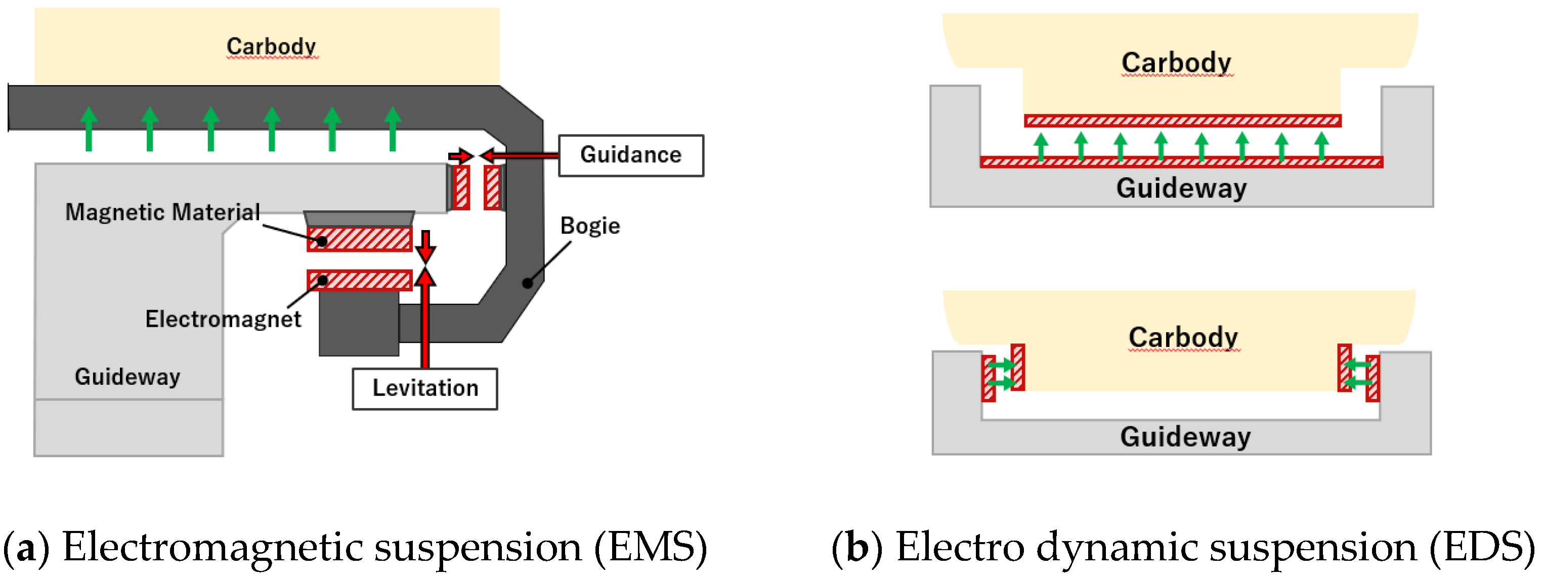
Funding

This research was supported by “Core Technology Development of Subsonic Capsule Train” of the Korea Railroad Research Institute under Grant PK2101A, Korea.

Conflicts of Interest

The authors declare no conflict of interest.

References

  1. Virgin Hyperloop One. Available online: https://virginhyperloop.com (accessed on 25 June 2021).
  2. Hyperloop Transportation Technology. Available online: https://www.hyperlooptt.com (accessed on 25 June 2021).
  3. Musk, E. Hyperloop Alpha; SpaceX: Hawthorne, CA, USA, 2013. [Google Scholar]
  4. Lever, J.H. (Ed.) Technical Assessment of Maglev System Concepts; US Army Corps of Engineers: Washington, DC, USA, 1998.
  5. Lee, H.-W.; Kim, K.-C.; Lee, J. Review of maglev train technologies. IEEE Trans. Magn. 2006, 42, 1917–1925. [Google Scholar]
  6. Yan, L. Development and application of the Maglev transportation system. IEEE Trans. Appl. Supercond. 2008, 18, 92–99. [Google Scholar]
  7. Kusagawa, S.; Baba, J.; Shutoh, K.; Masada, E. Multipurpose design optimization of EMS-type magnetically levitated vehicle based on genetic algorithm. IEEE Trans. Appl. Supercond. 2004, 14, 1922–1925. [Google Scholar] [CrossRef]
  8. Goodall, R.M. Generalised design models for EMS maglev. In Proceedings of the MAGLEV 2008, the 20th International Conference on Magnetically Levitated Systems and Linear Drives, San Diego, CA, USA, 15–18 December 2008, unpublished. [Google Scholar]
  9. Rote, D.M.; Cai, Y. A review of dynamic stability of repulsive-force maglev suspension systems. IEEE Trans. Magn. 2002, 38, 1383–1390. [Google Scholar] [CrossRef] [Green Version]
  10. Dai, H. Dynamic Behavior of Maglev Vehicle/Guideway System with Control. Electronic Thesis or Dissertation, Case Western Reserve University, Cleveland, OH, USA, 2005. OhioLINK Electronic Theses and Dissertations Center. [Google Scholar]
  11. Han, Q. Analysis and modeling of the EDS maglev system based on The Halbach permanent magnet array. Electronic Theses and Dissertations, University of Central Florida, Orlando, FL, USA, 2004. [Google Scholar]
  12. Korea Railroad Research Institute. Development of Core Technologies of Ultra-High-Speed Tube Train Project; Korea Railroad Research Institute Internal Report; Korea Railroad Research Institute: Uiwang-si, Korea, 2020. [Google Scholar]
  13. Choi, S.Y.; Lee, C.Y.; Jo, J.M.; Choe, J.H.; Oh, Y.J.; Lee, K.S.; Lim, J.Y. Sub-Sonic Linear Synchronous Motors Using Superconducting Magnets for the Hyperloop. Energies 2019, 12, 4611. [Google Scholar] [CrossRef] [Green Version]
  14. Lim, J.; Lee, C.-Y.; Lee, J.-H.; You, W.; Lee, K.-S.; Choi, S. Design Model of Null-Flux Coil Electrodynamic Suspension for the Hyperloop. Energies 2020, 13, 5075. [Google Scholar] [CrossRef]
  15. Lim, J.; Lee, C.-Y.; Choi, S.; Lee, J.-H.; Lee, K.-S. Design Optimization of a 2G HTS Magnet for Subsonic Transportation. IEEE Trans. Appl. Supercond. 2020, 30, 1–5. [Google Scholar] [CrossRef]
  16. He, J.L.; Rote, D.M.; Coffey, H.T. Study of Japanese Electrodynamic-Suspension Maglev Systems; Argonne National Lab.: Argonne, IL, USA, 1994.
  17. Erimitsu, S.; Jun, S.; Ken, W.; Hironori, H.; Masao, N. Comparison of methods to reduce vibrations in superconducting maglev vehicles by primary suspension control. J. Mech. Syst. Transp. Logist. 2008, 1, 3–13. [Google Scholar]
  18. Ken, W.; Hiroshi, Y.; Erimitsu, S.; Takayuki, T.; Masao, N. A study of vibration control systems for superconducting maglev vehicles (vibration control of lateral and rolling motions). J. Syst. Des. Dyn. 2007, 1, 593–604. [Google Scholar]
  19. Ken, W.; Hiroshi, Y.; Erimitsu, S.; Takayuki, T.; Masao, N. A study of vibration control systems for superconducting maglev vehicles (vibration control of vertical and pitching motions). J. Syst. Des. Dyn. 2007, 1, 703–713. [Google Scholar]
  20. Ohsaki, H.; Torii, S.; Higashi, K.; Masada, E. Damping Characteristics of the Superconductive Maglev Vehicle. In Advances in Superconductivity VI; Fujita, T., Shiohara, Y., Eds.; Springer: Tokyo, Japan, 1994. [Google Scholar]
  21. Ohashi, S.; Ohsaki, H.; Masada, E. Equivalent model of the side wall electrodynamic suspension system. Electr. Eng. Jap. 1998, 124, 63–73. [Google Scholar] [CrossRef]
  22. Takenori, Y.; Ken, W.; Erimitsu, S.; Takashi, S. Characteristics of Magnetic Springs for the Guidance of Superconducting Maglev Vehicles. Q. Rep. RTRI 2018, 54, 293–298. [Google Scholar]
  23. Shunsuke, F.; Tsuyoshi, F. Characteristics of combined levitation and guidance EDS maglev system. IEEJ Trans. Ind. Appl. 1992, 112, 459–466. [Google Scholar]
  24. Shunsuke, F.; Tsuyoshi, F. Characteristics of the combined levitation and guidance system using ground coils on the side wall of the guideway. In Proceedings of the International Conference on Magnetically Levitated Systems and Linear Drives, Yokohama, Japan, 7–11 July 1989. [Google Scholar]
  25. Yoon, R.; You, W.; Lee, J.; Lee, C.; Lee, K. Dynamic analysis of capsule train with 9-dof according to speed. J. Korean Soc. Railw. 2019, 22, 109–117. [Google Scholar] [CrossRef]
  26. Yoon, R.; You, W.; Lee, J.; Lee, C.; Lee, K. Study on dynamic characteristics of superconducting capsule train. Trans. Korean Soc. Noise Vib. Eng. 2019, 29, 453–461. [Google Scholar] [CrossRef]
  27. Guest, P.G. Numerical Methods of Curve Fitting; Cambridge University Press: Cambridge, UK, 2012. [Google Scholar]
  28. Arlinghaus, S. Practical Handbook of Curve Fitting; CRC Press: Boca Raton, FL, USA, 1994. [Google Scholar]
  29. William, S. Practical curve fitting. Assoc. Sci. Limnol. Oceanogr. 1979, 24, 767–773. [Google Scholar]
  30. Yang, Y.B.; Yau, J.D.; Wu, Y.S. Vehicle-Bridge Interaction Dynamics; World Scientific: Singapore, 2004; pp. 303–309. [Google Scholar]
  31. Lei, X.; Chen, X.; Li, X.; Meng, X. Track irregularity spectrum analysis of Shenchi-Huanghua heavy haul railway. J. Cent. South Univ. 2013, 12, 5147–5153. [Google Scholar]
  32. Deng, Z.; Wang, L.; Li, H.; Li, J.; Wang, H.; Yu, J. Dynamic studies of the HTS maglev transit system. IEEE Trans. Appl. Supercond. 2021, 31, 1–5. [Google Scholar]
Figure 1. Principle of electromagnetic suspension and electro dynamic suspension.
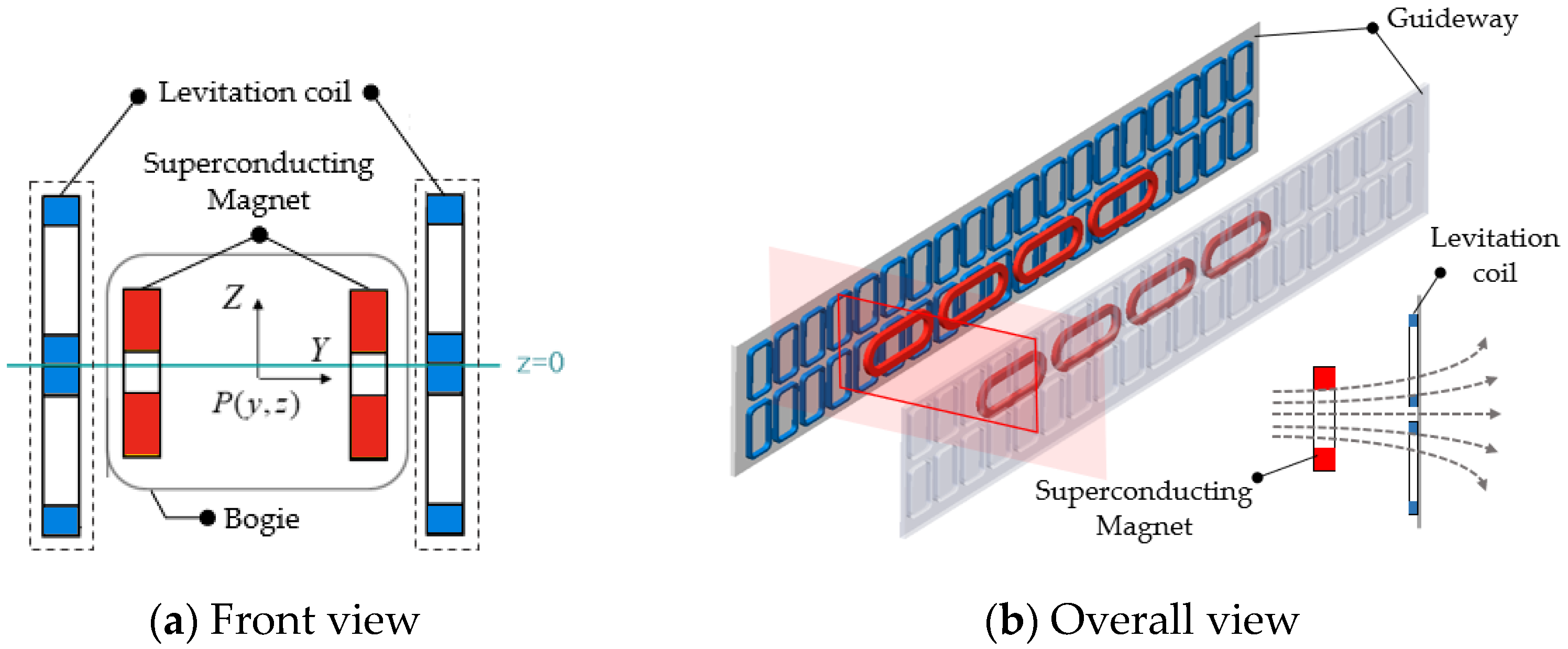
Energies 14 04979 g001
Figure 2. Arrangement of superconducting magnets and levitation coil.
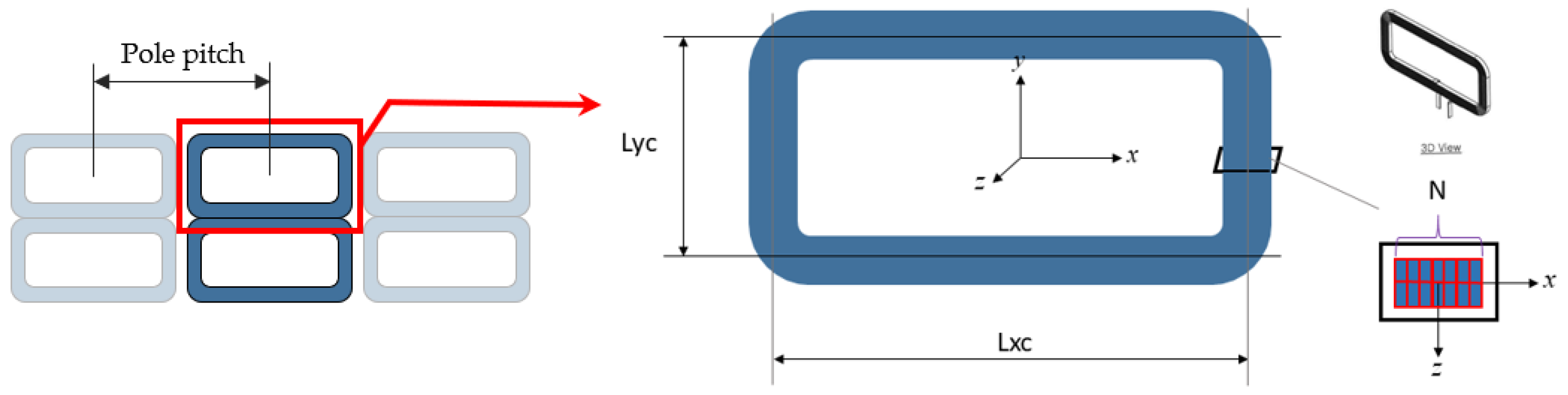
Energies 14 04979 g002
Figure 3. Design of levitation coil.
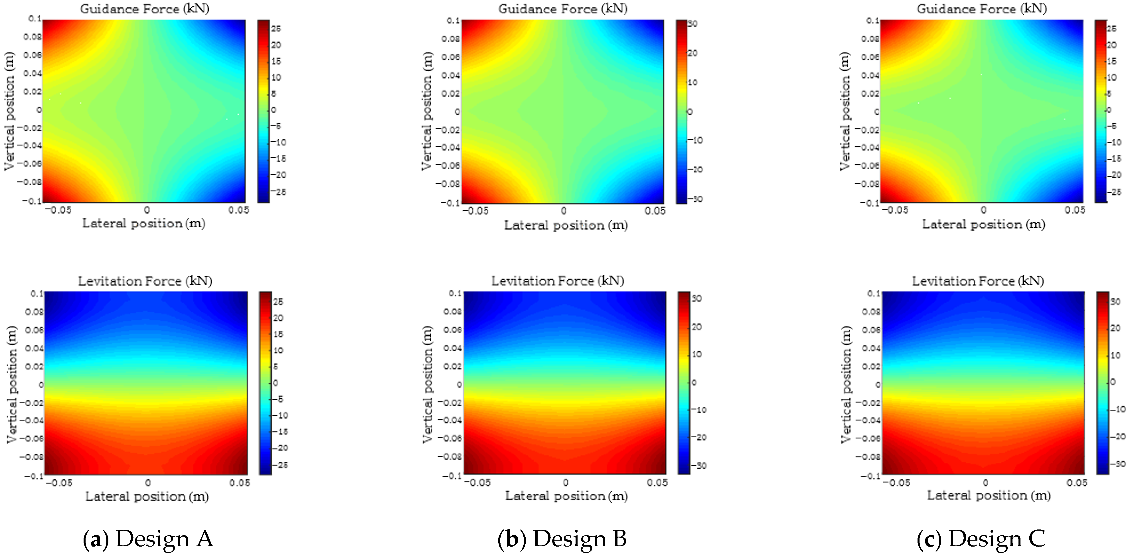
Energies 14 04979 g003
Figure 4. Distributions of the guidance and levitation forces.
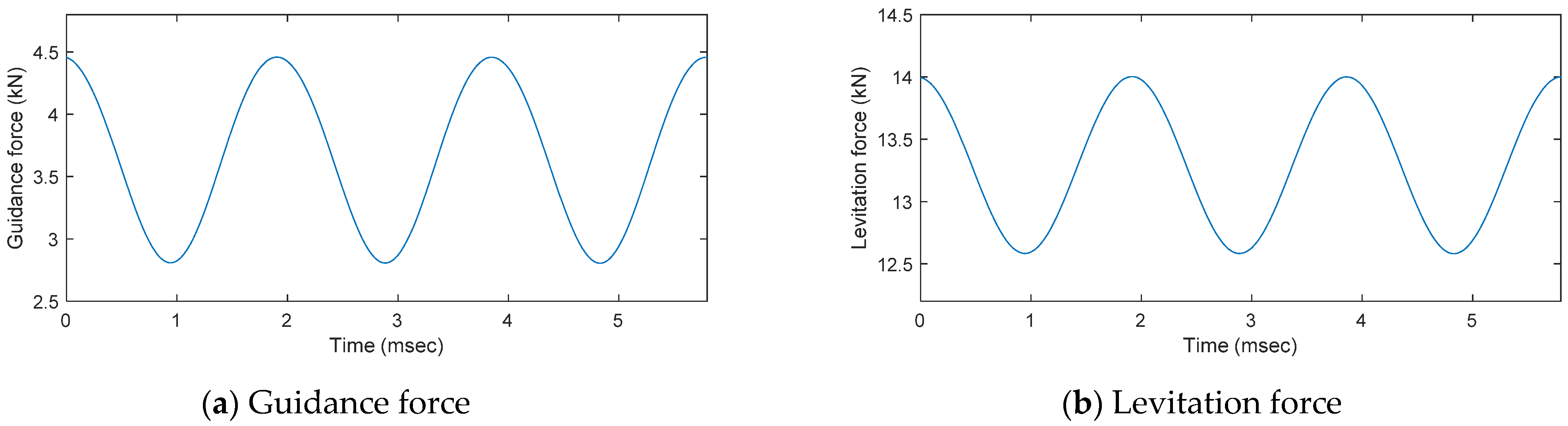
Energies 14 04979 g004
Figure 5. Levitation/guidance force in the time domain (Design A).
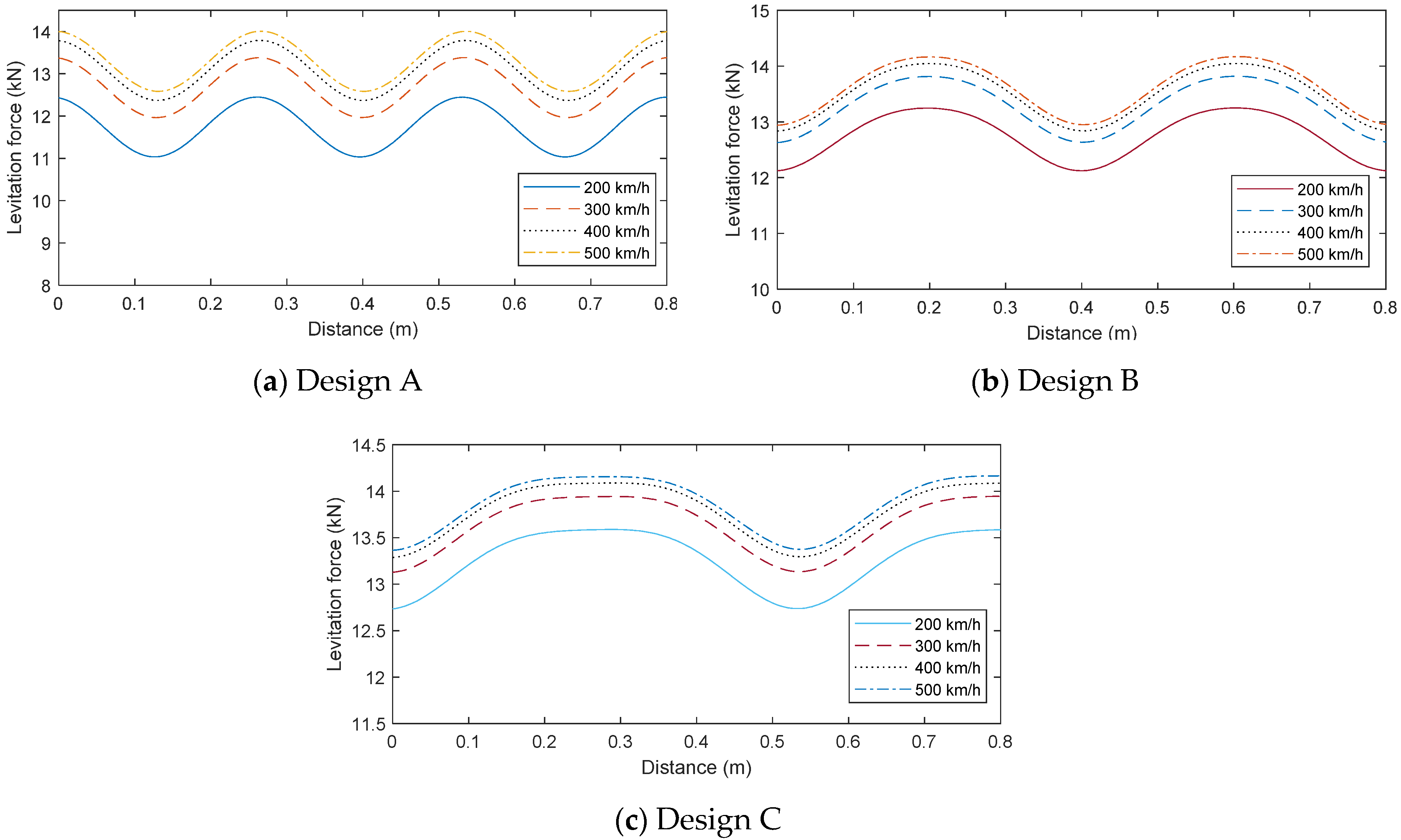
Energies 14 04979 g005
Figure 6. Variation in the levitation force with respect to vehicle speed.
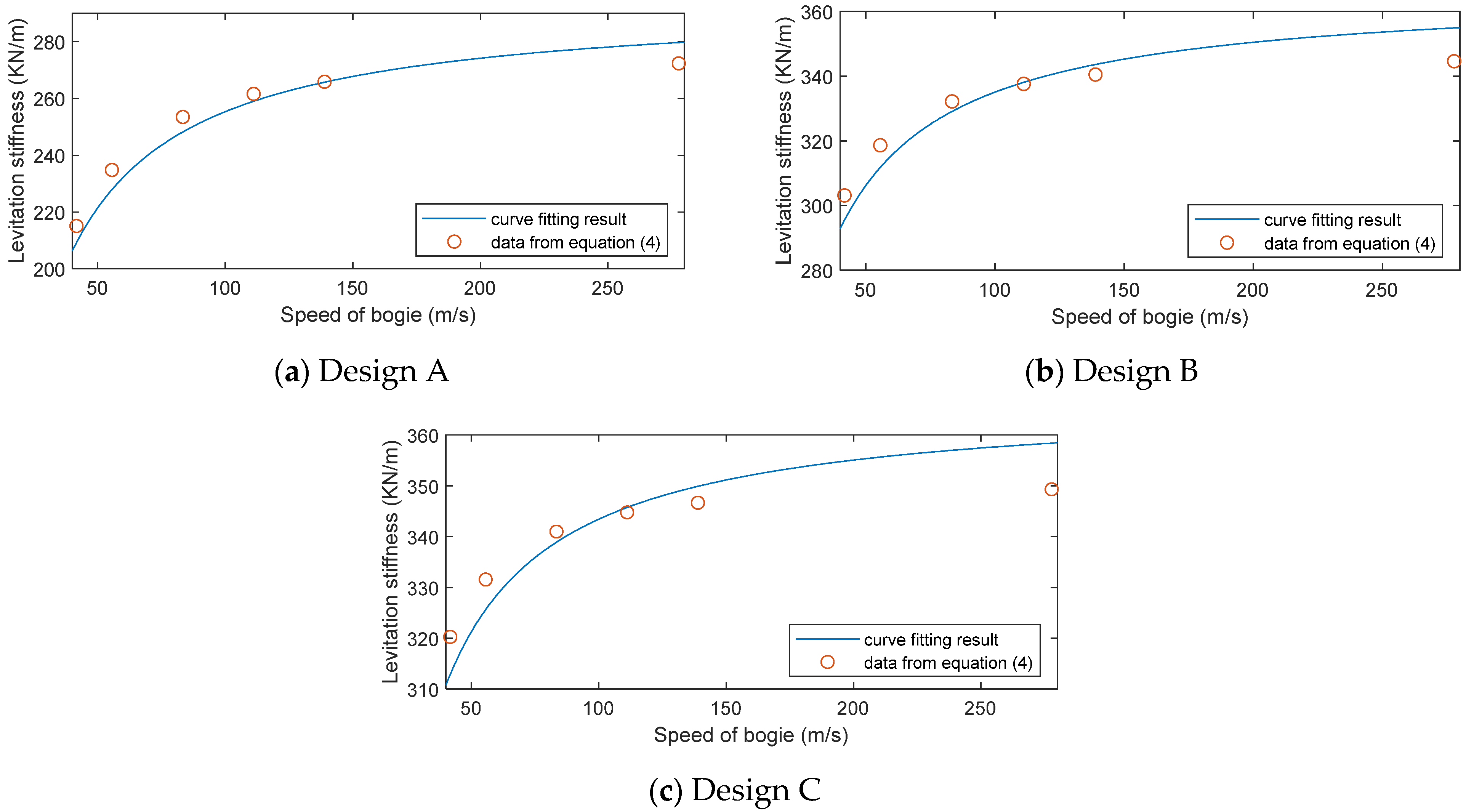
Energies 14 04979 g006
Figure 7. Levitation stiffness with respect to the speed of the traveling body.
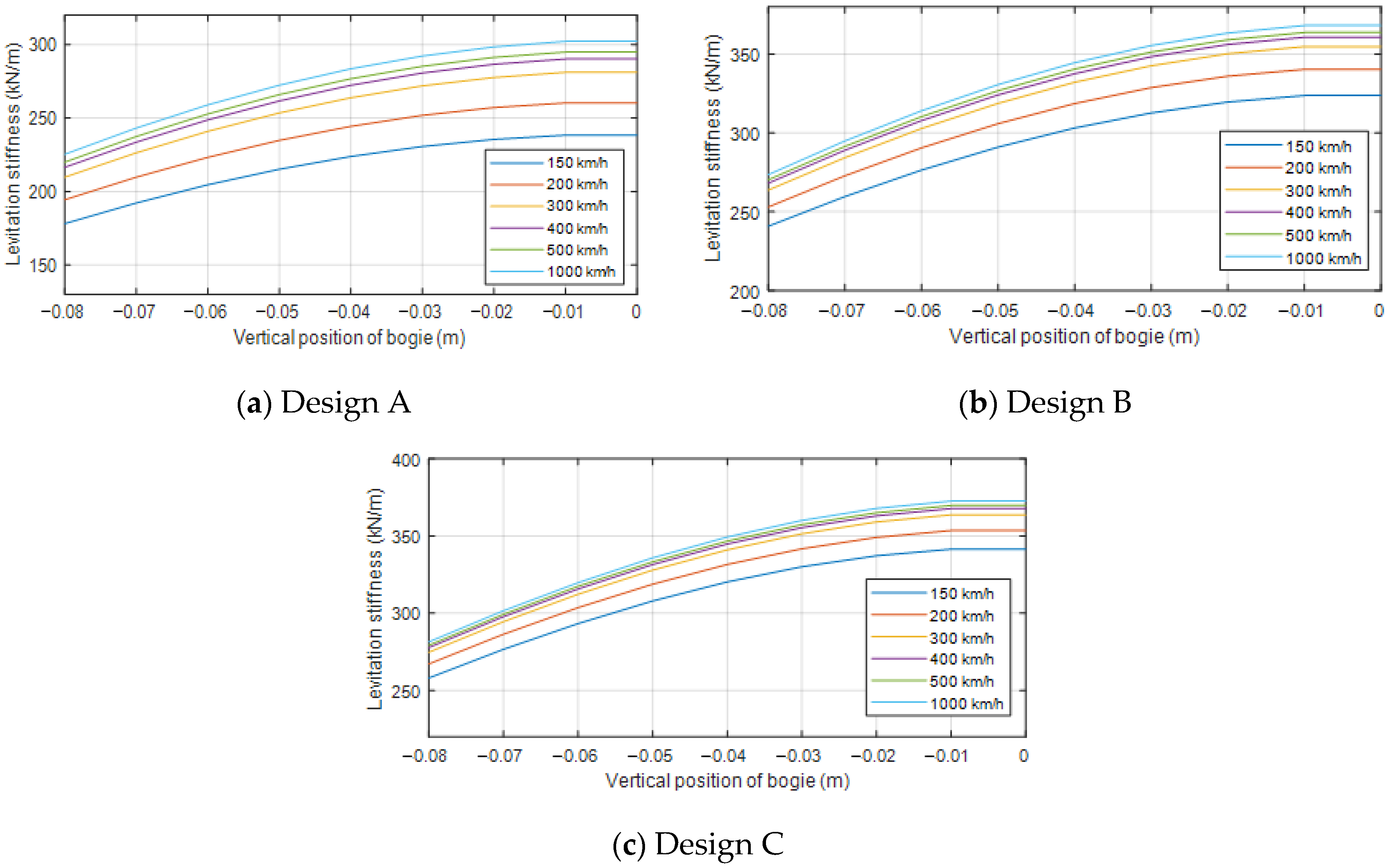
Energies 14 04979 g007
Figure 8. Relationship between levitation stiffness and vertical position (average).
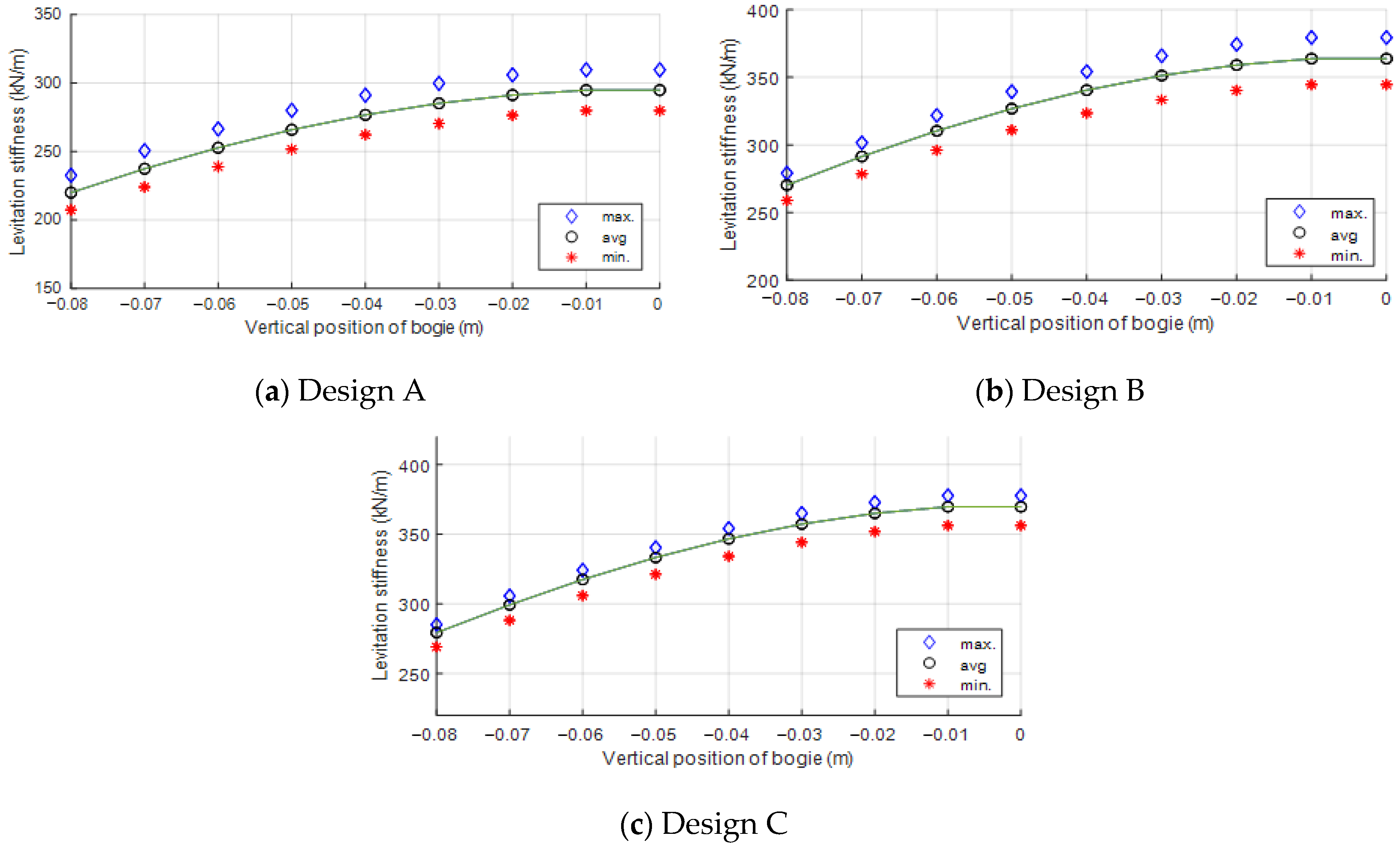
Energies 14 04979 g008
Figure 9. Relationship between levitation stiffness and vertical position (average and fluctuation).
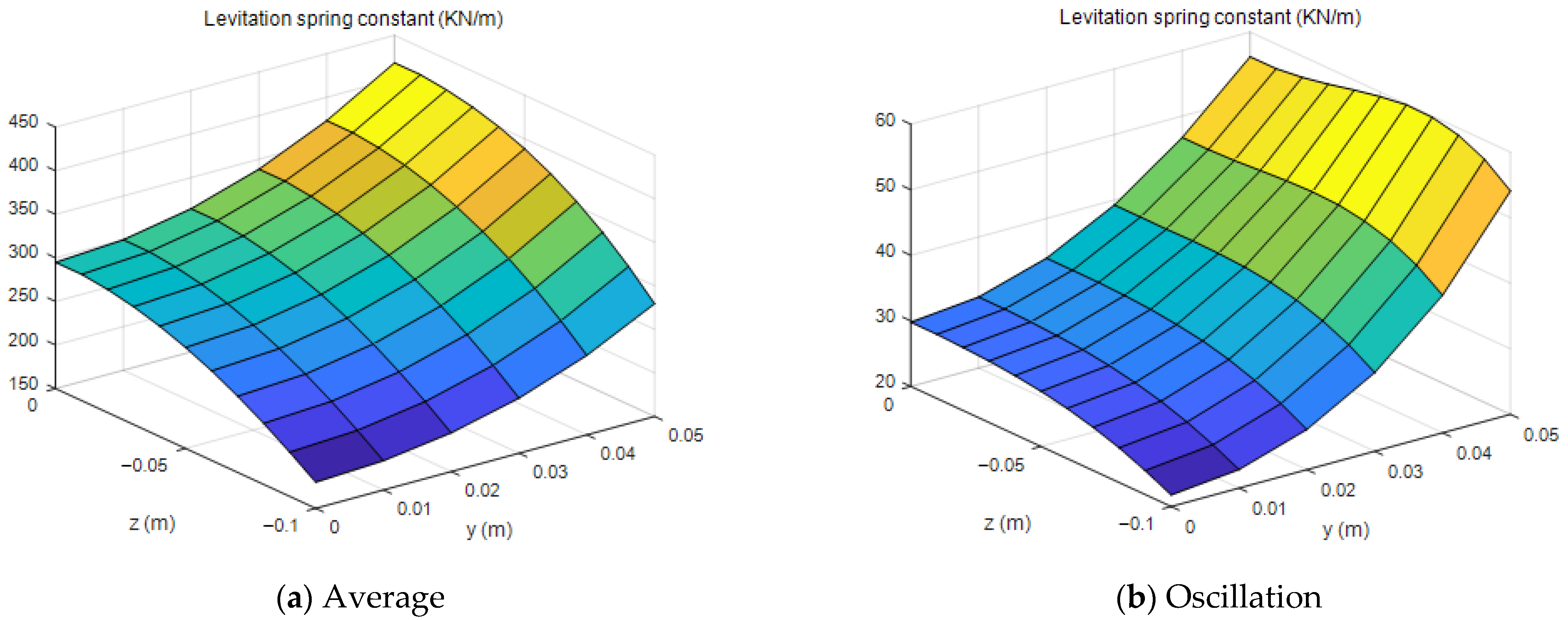
Energies 14 04979 g009
Figure 10. Levitation stiffness with respect to vertical and lateral positions.
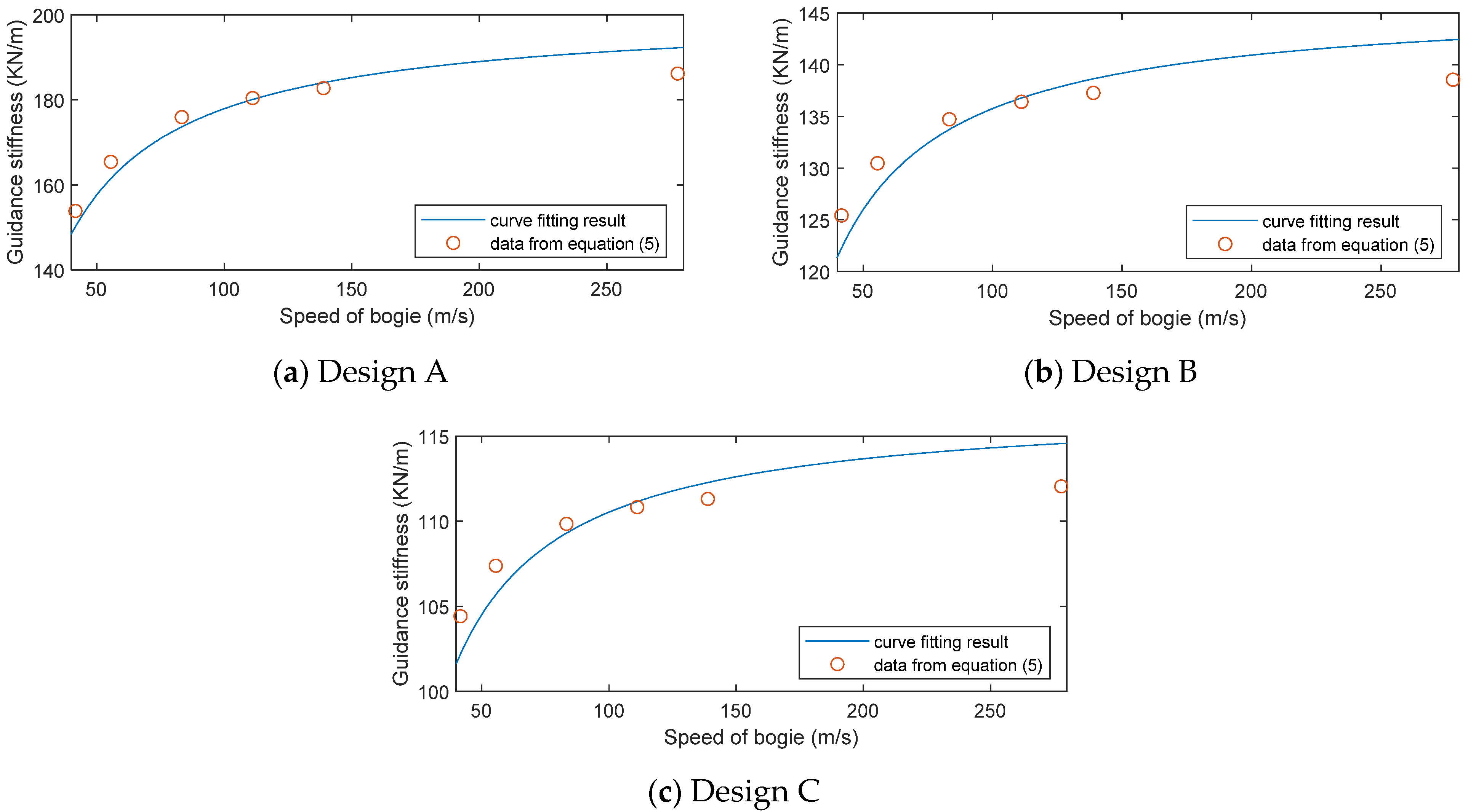
Energies 14 04979 g010
Figure 11. Guidance stiffness with respect to the speed of the traveling body.
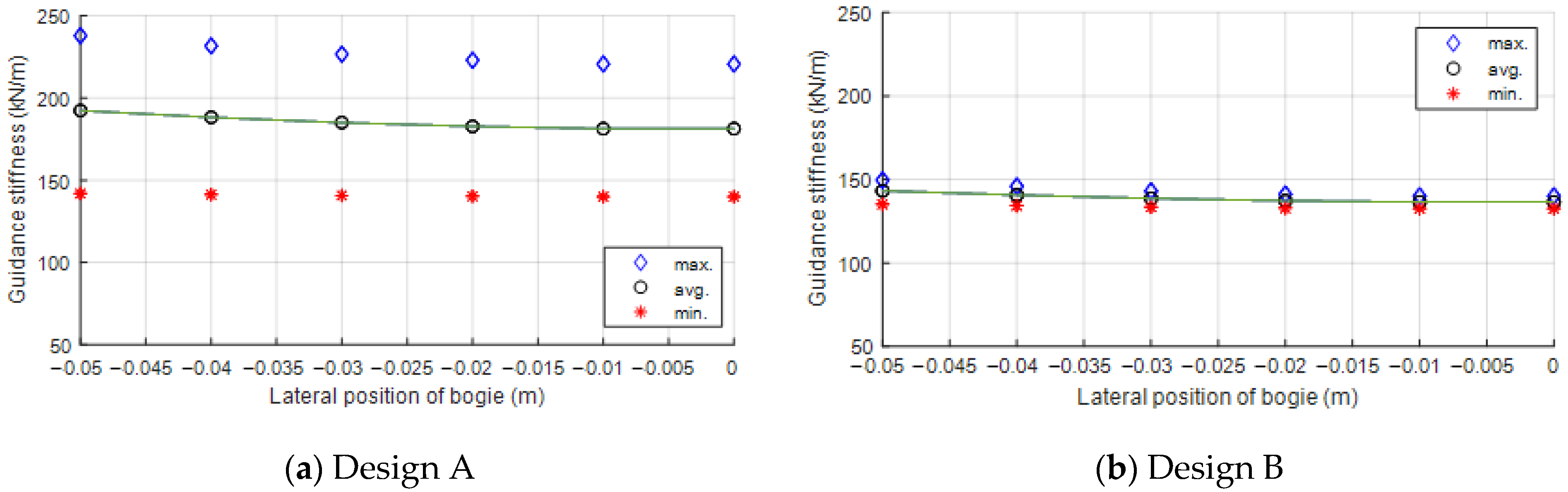
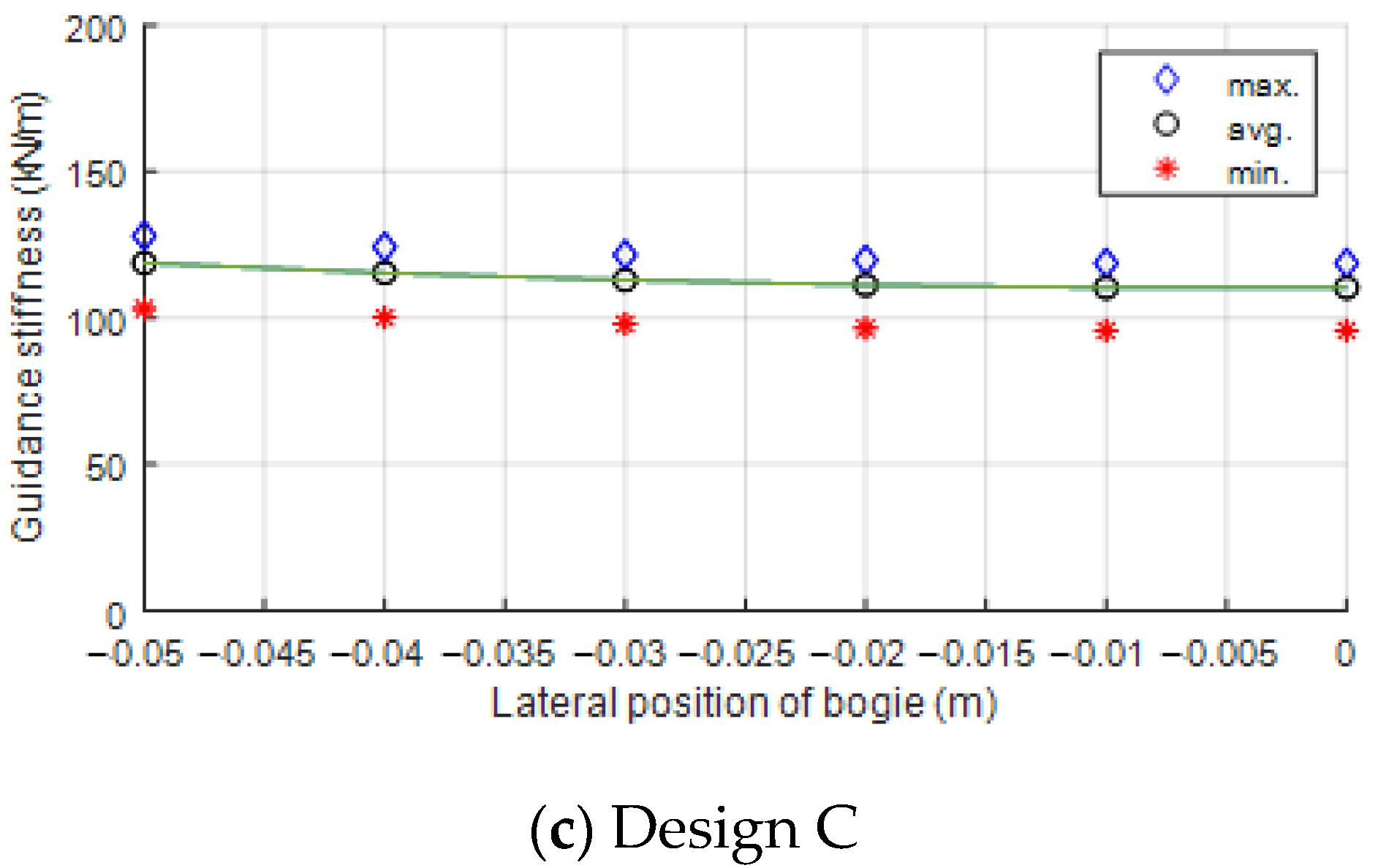
Energies 14 04979 g011
Figure 12. Relationship between guidance stiffness and lateral position (average).
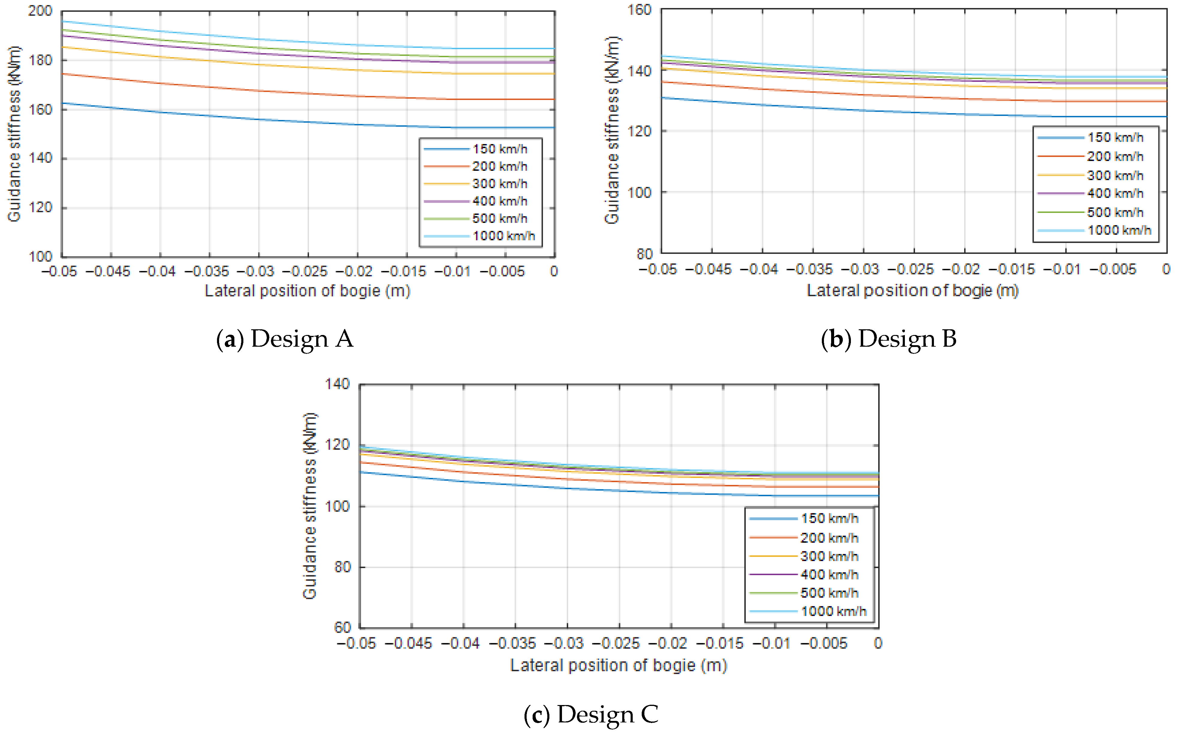
Energies 14 04979 g012
Figure 13. Relationship between the guidance stiffness and the lateral position (average and fluctuation).
Energies 14 04979 g013aEnergies 14 04979 g013b
Figure 14. Guidance stiffness with respect to the vertical and lateral positions.
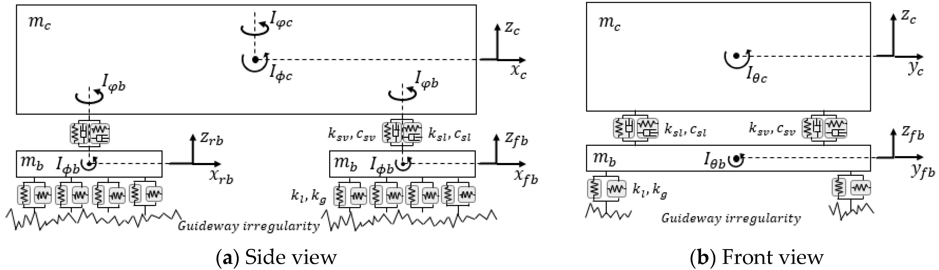
Energies 14 04979 g014
Figure 15. Dynamic model of the capsule train with the main parameters.
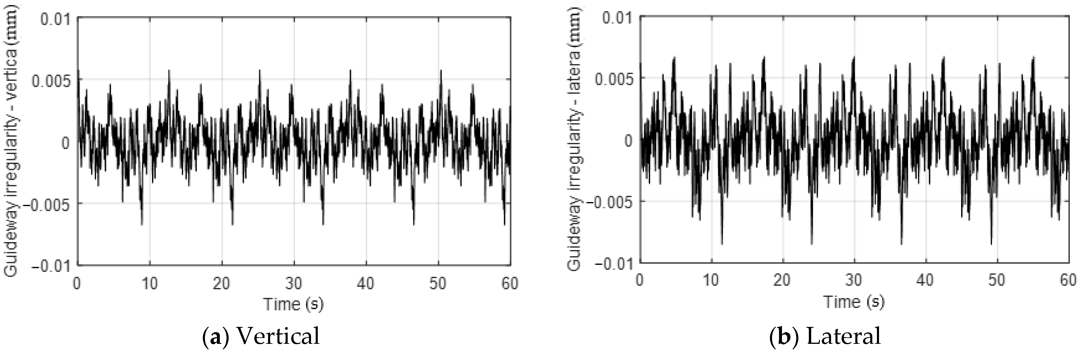
Energies 14 04979 g015
Figure 16. Guideway irregularity in the vertical/lateral direction.
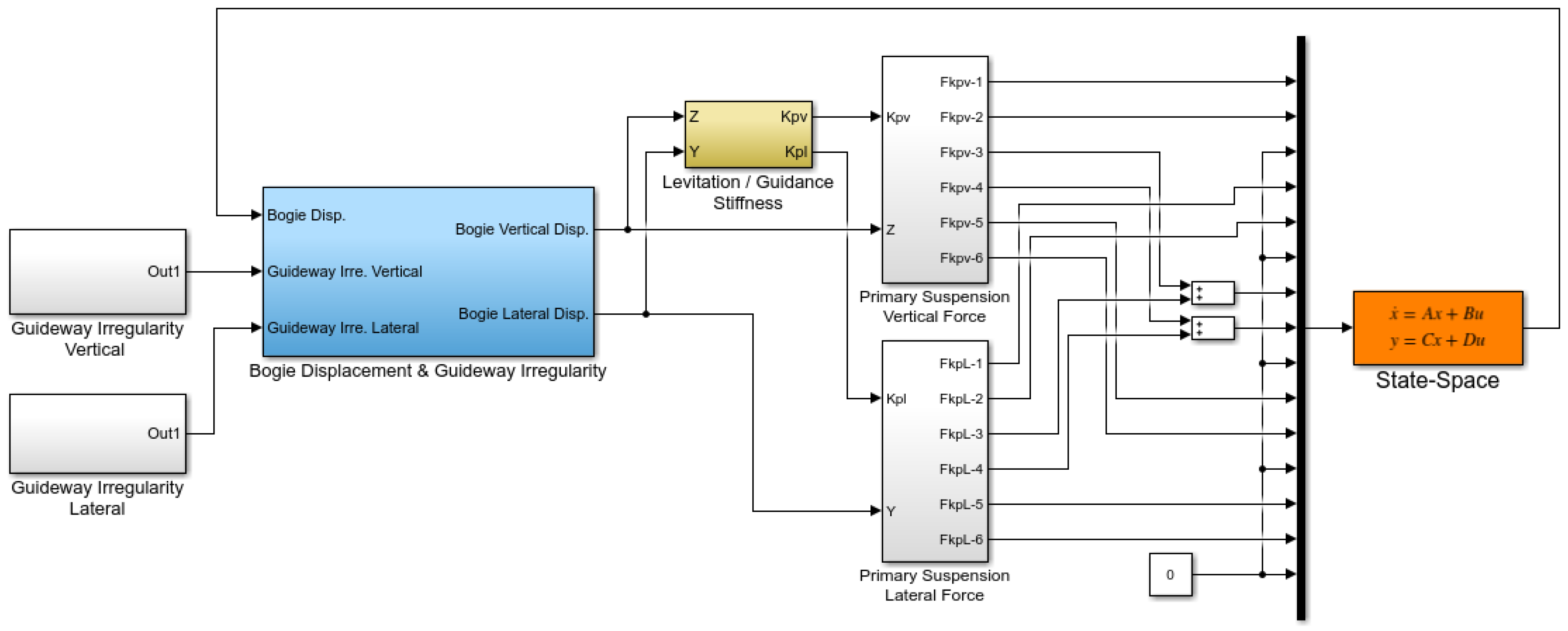
Energies 14 04979 g016
Figure 17. Modeling of capsule vehicle with Simulink S/W.
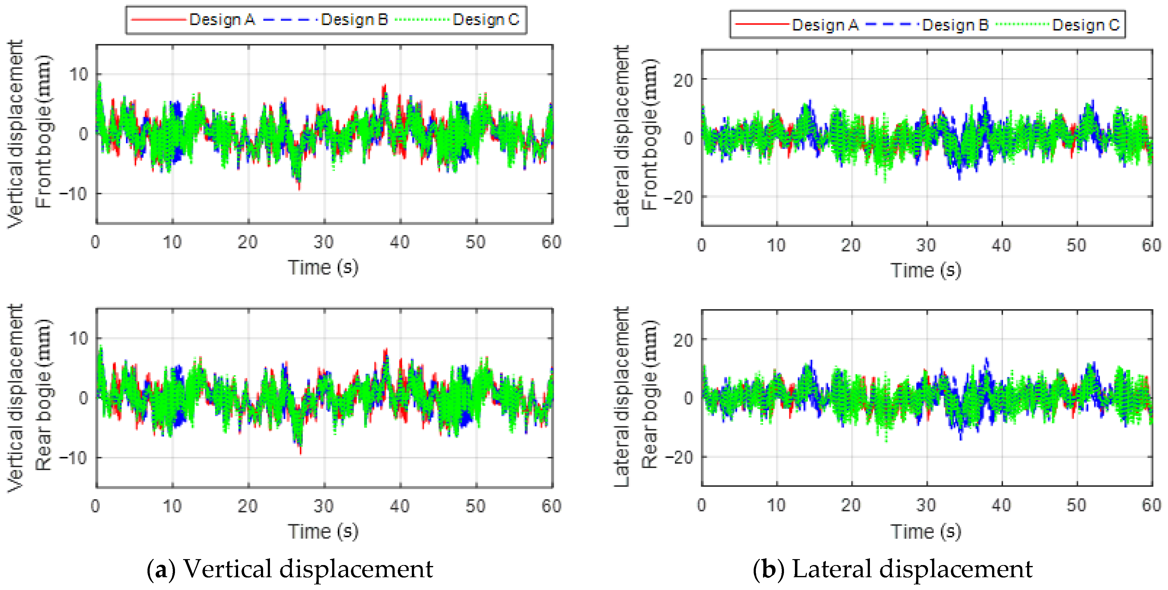
Energies 14 04979 g017
Figure 18. Vertical and lateral displacements of the front and rear bogies at a speed of 300 km/h.
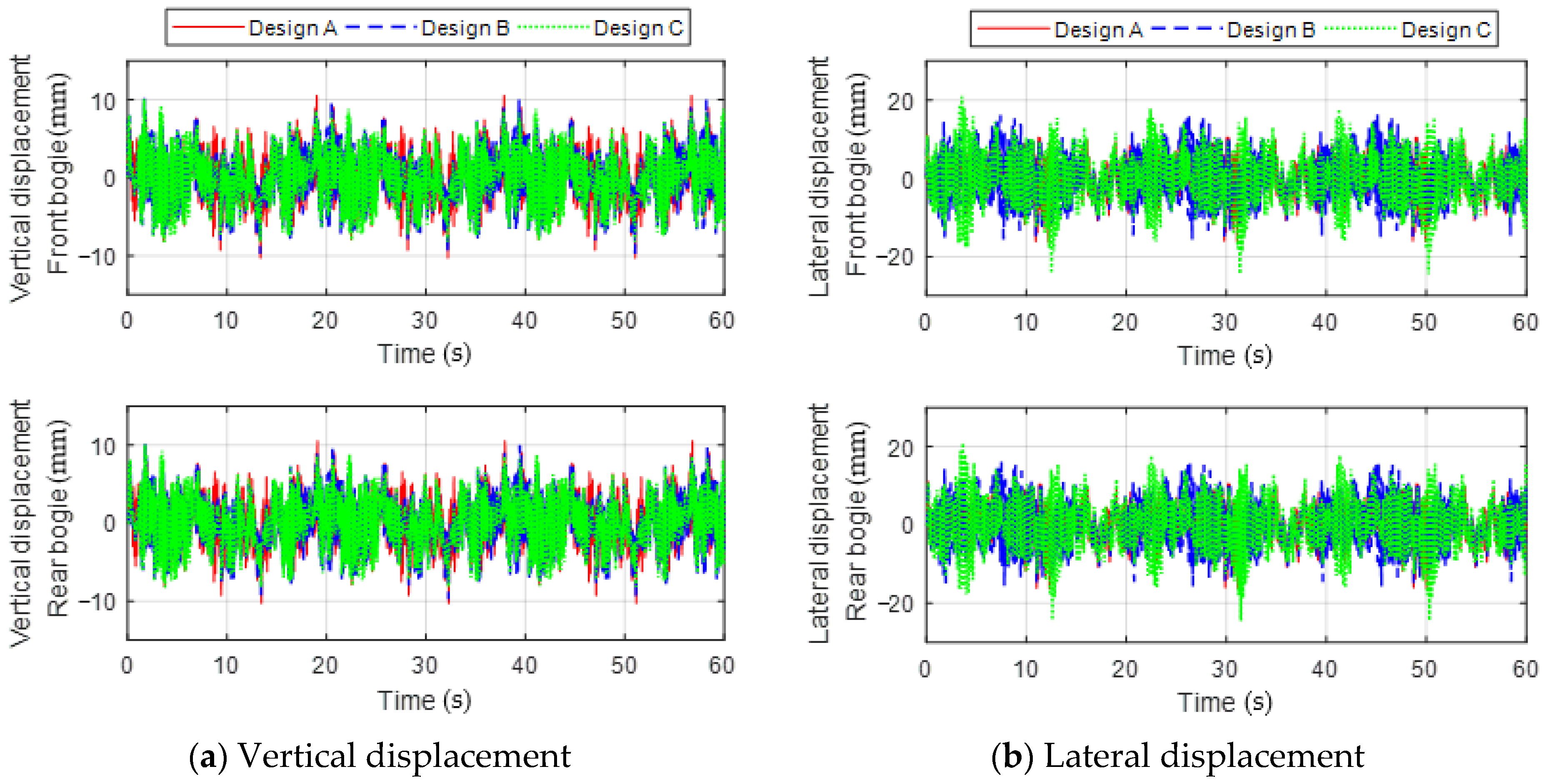
Energies 14 04979 g018
Figure 19. Vertical and lateral displacements of the front and rear bogies at a speed of 600 km/h.
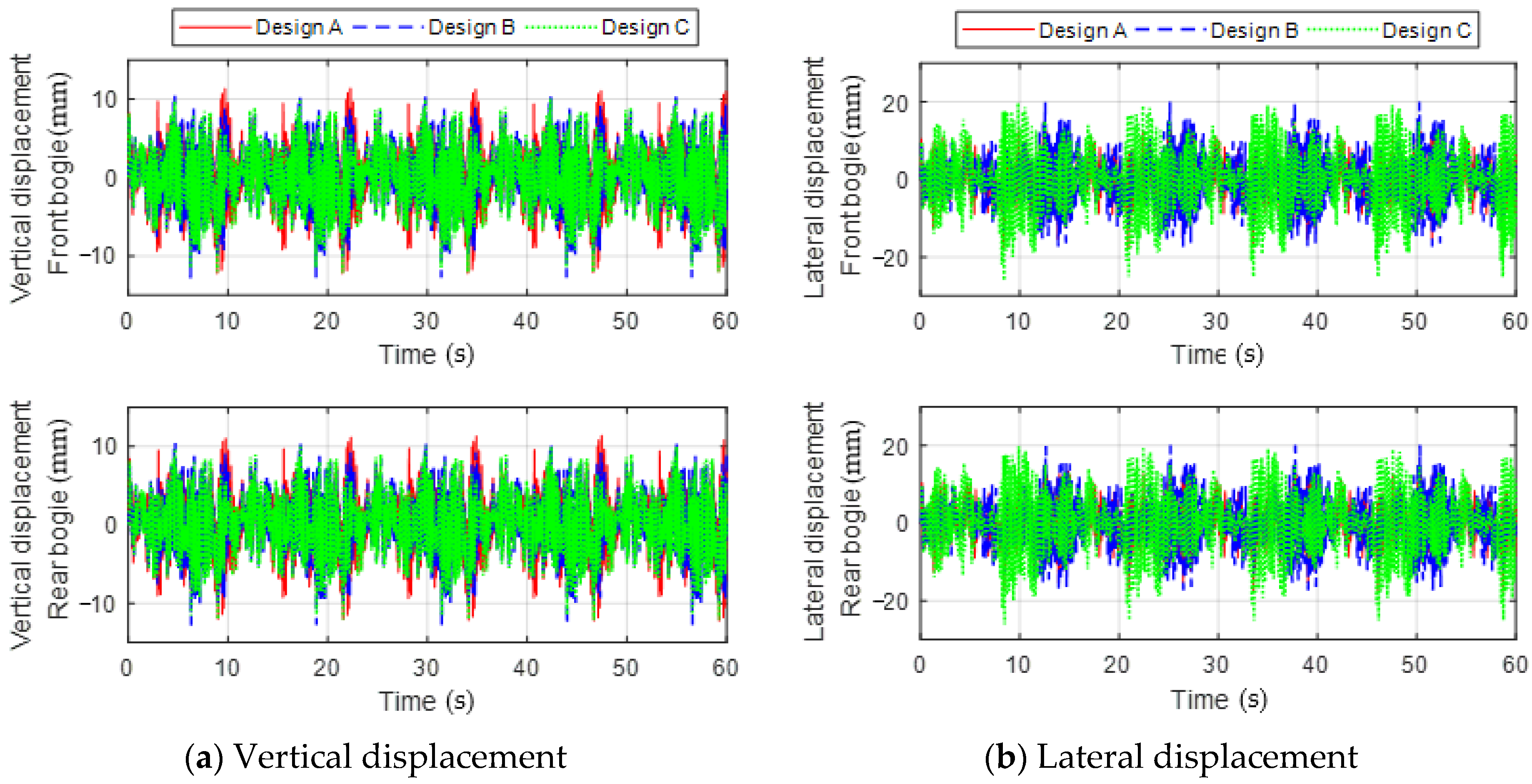
Energies 14 04979 g019
Figure 20. Vertical and lateral displacements of the front and rear bogies at a speed of 900 km/h.
Energies 14 04979 g020
Figure 21. RMS value of the vertical/lateral displacements of the bogie with respect to speed.
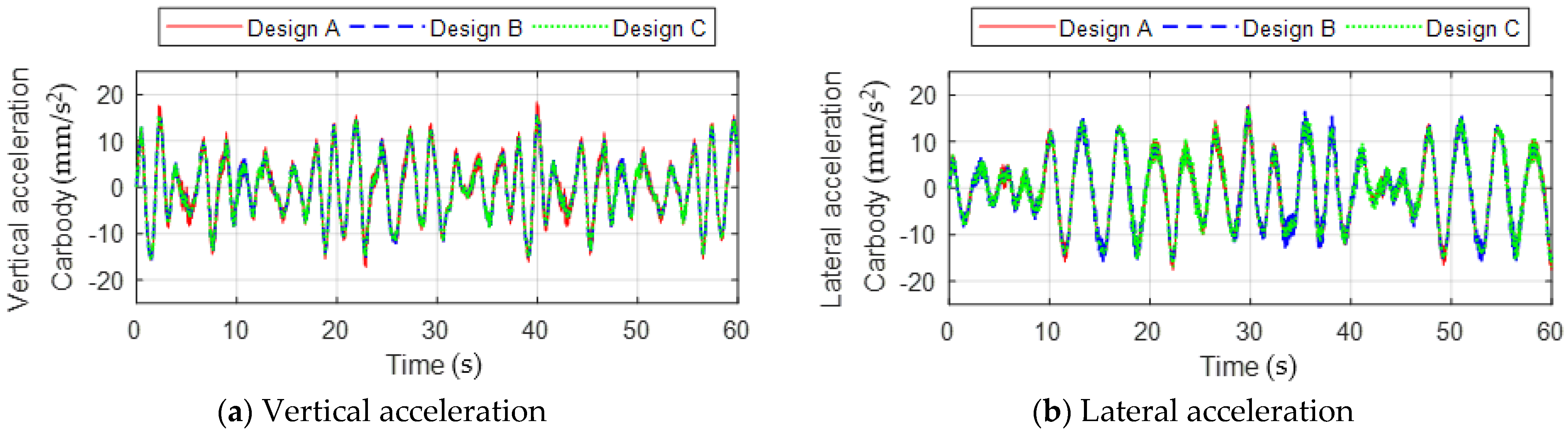
Energies 14 04979 g021
Figure 22. Vertical and lateral accelerations of a carbody at a speed of 300 km/h.
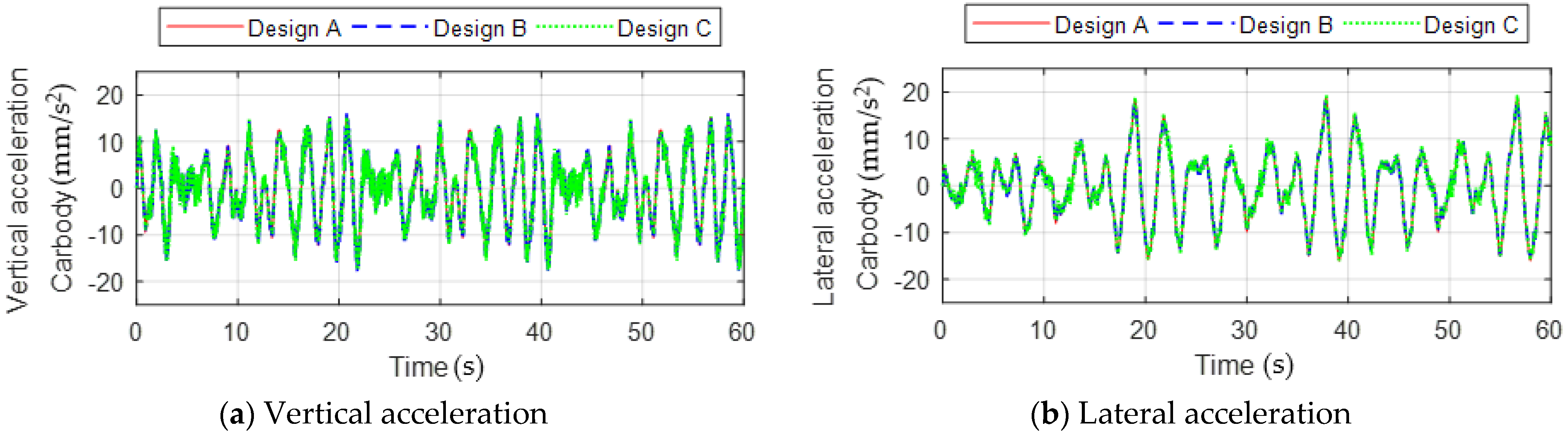
Energies 14 04979 g022
Figure 23. Vertical and lateral accelerations of the carbody at a speed of 600 km/h.
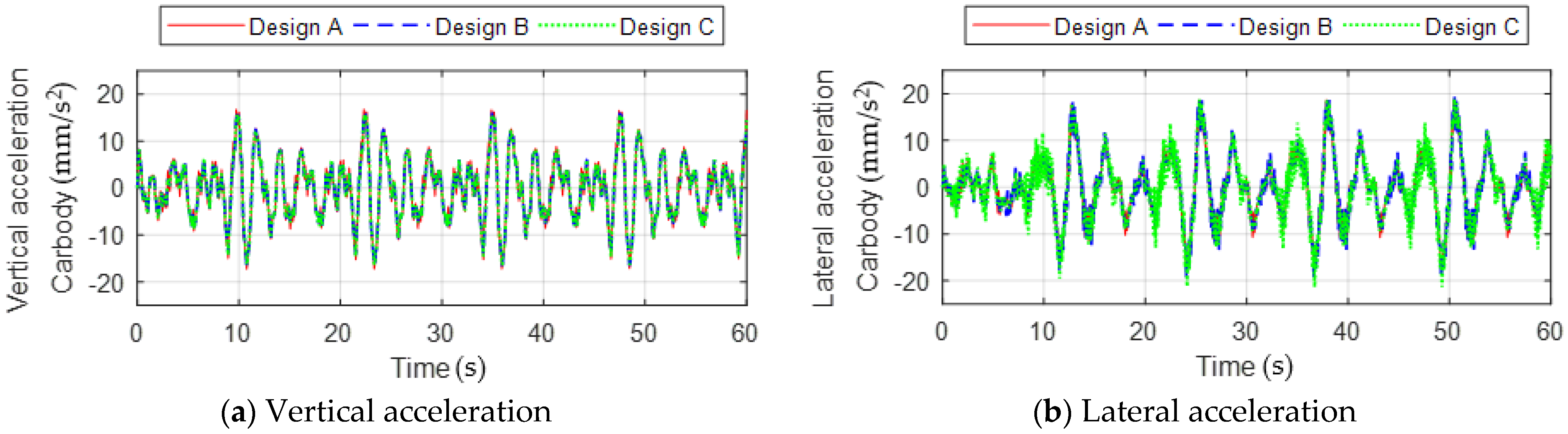
Energies 14 04979 g023
Figure 24. Vertical and lateral accelerations of a carbody at a speed of 900 km/h.
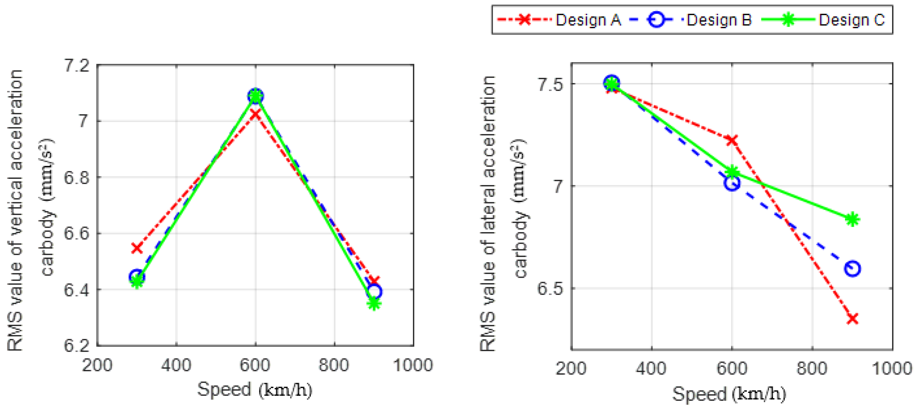
Energies 14 04979 g024
Figure 25. RMS value of the vertical/lateral acceleration with respect to speed.
Energies 14 04979 g025
Table 1. Design models of levitation coil.
DesignPole Pitch (mm)Lxc (mm)Lyc (mm)Number of Turns in the Coil
A27018029012
B40528528018
C54039028024
Table 2. Balance position of levitation force.
Position z (m)Levitation Force (kN)
Design ADesign BDesign C
−0.038.553910.539210.7192
−0.0411.069213.554913.7655
−0.0513.292016.261316.5397
Table 3. Average value and fluctuation in levitation/guidance force.
DesignDesign ADesign BDesign C
Levitation force (kN)Average13.292013.554913.7655
Fluctuation (0–peak)0.71060.61500.4010
Rate of fluctuation (%)5.354.542.91
Guidance force (kN)Average3.63242.73992.1630
Fluctuation (0–peak)0.82710.08270.2331
Rate of fluctuation (%)22.773.0210.78
Table 4. Parameter values of levitation stiffness.
ParameterDesign ADesign BDesign C
a z 264,400366,600367,100
b z 14.228.996.66
Table 5. Coefficients of levitation stiffness (average and oscillation).
Design Average   ( k z , a v g ) Oscillation   ( k z , o s c ) τ l
A c 1 = 327.1 × 10 3 e ( 14.22 / v ) c o 1 = 16.67 × 10 3 e ( 14.22 / v ) 0.270
c 2 = 1.291 × 10 7 e ( 14.22 / v ) c o 2 = 0.044 × 10 7 e ( 14.22 / v )
B c 1 = 388.02 × 10 3 e ( 8.99 / v ) c o 1 = 18.30 × 10 3 e ( 8.99 / v ) 0.405
c 2 = 1.533 × 10 7 e ( 8.99 / v ) c o 2 = 0.11 × 10 7 e ( 8.99 / v )
C c 1 = 387.23 × 10 3 e ( 6.66 / v ) c o 1 = 11.23 × 10 3 e ( 6.66 / v ) 0.540
c 2 = 1.445 × 10 7 e ( 6.66 / v ) c o 2 = 0.041 × 10 7 e ( 6.66 / v )
Table 6. Mathematical expressions of the levitation stiffness.
DesignEquation l v d
A k l , y z = ( 5.40 195.4 ( z + l v ) 2 ) ( 54.42 + 10 4 y 2 ) × 10 3 × e ( d / v )
k l , y z , o s c = ( 0.629 7.696 ( z + l v ) 2 ( 2255 + 10 4 y 2 ) × 10 3 × e ( d / v )
0.0514.22
B k l , y z = ( 6.5 244.7 ( z + l v ) 2 ) ( 55.71 + 10 4 y 2 ) × 10 3 × e ( d / v )
k l , y z , o s c = ( 1.01 62.01 ( z + l v ) 2 ) ( 16.63 + 10 4 y 2 ) × 10 3 × e ( d / v )
0.048.99
C k l , y z = ( 6.1 223.3 ( z + l v ) 2 ) ( 60.21 + 10 4 y 2 ) × 10 3 × e ( d / v )
k l , y z , o s c = ( 0.098 3.336 ( z + l v ) 2 ) ( 107.7 + 10 4 y 2 ) × 10 3 × e ( d / v )
0.046.66
Table 7. Parameter values of guidance stiffness.
ParameterDesign ADesign BDesign C
a y 200,800146,300116,900
b y 12.097.485.60
Table 8. Coefficients of the guidance stiffness (average and oscillation).
Design Average   ( k y , a v g ) Oscillation   ( k y , o s c ) τ l
A d 1 = 197.57 × 10 3 e ( 12.09 / v ) d o 1 = 43.65 × 10 3 e ( 12.09 / v ) 0.270
d 2 = 0.491 × 10 6 e ( 12.09 / v ) d o 2 = 3.426 × 10 6 e ( 12.09 / v )
B d 1 = 143.84 × 10 3 e ( 7.48 / v ) d o 1 = 3.799 × 10 3 e ( 7.48 / v ) 0.405
d 2 = 2.909 × 10 7 e ( 7.48 / v ) d o 2 = 1.490 × 10 7 e ( 7.48 / v )
C d 1 = 114.63 × 10 3 e ( 5.60 / v ) d o 1 = 11.96 × 10 3 e ( 5.60 / v ) 0.540
d 2 = 3.566 × 10 7 e ( 5.60 / v ) d o 2 = 0.389 × 10 7 e ( 5.60 / v )
Table 9. Mathematical expressions of the guidance stiffness.
DesignEquation l v d
A k g , y z = ( 0.279 + 191.9 ( z + l v ) 2 ) ( 230.8 + 10 4 y 2 ) × 10 3 × e ( d / v ) k g , y z , o s c = ( 0.24 + 53.64 ( z + l v ) 2 ) ( 107.2 + 10 4 y 2 ) × 10 3 × e ( d / v ) 0.0512.09
B k g , y z = ( 0.201 + 217.9 ( z + l v ) 2 ) ( 239.2 + 10 4 y 2 ) × 10 3 × e ( d / v ) k g , y z , o s c = ( 0.084 + 73.44 ( z + l v ) 2 ) ( 54.06 + 10 4 y 2 ) × 10 3 × e ( d / v ) 0.047.48
C k g , y z = ( 0.115 + 196.0 ( z + l v ) 2 ) ( 247.3 + 10 4 y 2 ) × 10 3 × e ( d / v ) k g , y z , o s c = ( 0.02 + 1.84 ( z + l v ) 2 ) ( 510.26 + 10 4 y 2 ) × 10 3 × e ( d / v ) 0.045.60
Table 10. Parameters of the capsule vehicle for simulation.
ParameterValueParameterValue
m b 4759   kg I Ø b 283,300   kg · m 2
m c 17,060   kg I φ b 283,300   kg · m 2
I θ c 17,100   kg · m 2 k s v 18,630   N / m
I Ø c 1,090,000   kg · m 2 k s l 16,670   N / m
I φ c 1,070,000   kg · m 2 c s v 1863   Ns / m
I θ b 2495   kg · m 2 c s l 833.5   Ns / m
Publisher’s Note: MDPI stays neutral with regard to jurisdictional claims in published maps and institutional affiliations.

