A Visual Software Implementation of Numerical Simulation for Transient Process of Pipeline Network System of Water Supply Project

Abstract

The transient process is the key for the design, operation and maintenance of the pipeline network system of the water supply project. This paper aims to study and develop a new type of visual numerical simulation software for the transient process of pipeline network system. Firstly, the software architecture design is illustrated. Then, three tiers of software architecture, i.e., back-tier, middle-tier and front-tier, are studied and developed. Finally, the practical application procedure of the software is illustrated and the accuracy of calculation results is verified. The results indicate that the visual numerical simulation software is designed based on C/S architecture. The software architecture contains back-tier, middle-tier and front-tier. The back-tier includes the model and the algorithm. The middle-tier realizes the decoding of the topology of the pipeline network system and the interaction between the back-tier and the front-tier. The front-tier integrates the visual interface and pre-post processing. The main interface includes a menu bar, a visual modeling area and a parameter input dialog box. The software has the features of professionalization, visualization, generalization, modularization and intellectualization. The software can calculate the transient process for the pipeline network system of both, pressure flow without the pump and pressure flow with the pump. The physical laws reflected from the calculation results are correct. The calculation results are accurate.

1. Introduction

The water supply project is an infrastructure for the transmission and distribution of water resources for living and production [1,2]. Generally, a water supply project contains reservoirs, pipelines, pumps, valves and water hammer prevention facilities. The types of water supply projects usually include a pressure flow system without a pump, a pressure flow system with a pump and a mixed water supply system [3,4].

The water supply project generally consists of a complex pipeline network system. Based on the theories of transient flow, the hydraulic design and optimization of the pipeline network system are the basis for the construction and operation of water supply projects [5,6]. Moreover, the hydraulic design and optimization are based on the calculation and analysis of transient processes [7,8,9]. The transient process is the key aspect for the design, operation and maintenance of the pipeline network system of the water supply project. According to the calculation and analysis results of the transient process, the design guidelines, optimization methods and operation strategies can be obtained for the pipeline network system.

The focus of the calculation and analysis of the transient process is the water hammer. The water hammer phenomenon widely exists in the pipeline network system of water supply projects. The methods for the calculation of the transient process usually include the analytical method, the graphical method and the numerical method [10,11]. Zhukovsky [12] proposes the computational formula of a direct water hammer, which establishes the relationship between a decrease of flow speed and an increase of water pressure. Gibson [13] considers the nonlinear friction losses in the analysis of water hammer and investigates the calculation of pressures in penstocks caused by gradual closing of turbine gates. Allievi [14] proposes the computational formula of indirect water hammer. In that formula, the water hammer constant is introduced. Schnyder [15] studies the calculation of water hammer by using graphical analysis and includes the friction losses first. Bergeron [16] investigates the decay of self-excited oscillations for a normal or a leaking valve by using a graphical water hammer analysis. The analytical and graphical methods establish the theoretical basis of the water hammer. However, those two methods are just used to deal with simple pipeline network systems [17,18,19]. The results obtained from the analytical and graphical methods are usually approximate solutions. Therefore, the analytical and graphical methods have a great limitation. In general, the numerical method is the first choice for the calculation of the transient process because the numerical method can deal with complex pipeline network systems and has high accuracy [20,21,22,23]. The classical method for the numerical calculation of the transient process is the method of characteristics. In [24], Fox introduces the basic equations, principle, derivation, zone and boundary conditions of the method of characteristics in detail. In [25], Goldberg and Wylie improve the application of the method of characteristics to wave problems in hydraulics by using the interpolations in time.

With the rapid development of computer technology, the numerical method for the calculation of the transient process becomes more and more popular. At present, the numerical calculation of the transient process mainly contains the one-dimensional numerical solution and three-dimensional numerical solution [26,27,28,29,30]. Compared with the three-dimensional numerical solution, the one-dimensional numerical solution has enough accuracy. Moreover, for the one-dimensional numerical solution, fewer computing resources and computing time are spared, and the computing processes are much simpler [31,32]. Therefore, the one-dimensional numerical solution is the research emphasis of the numerical calculation of the transient process. However, the traditional one-dimensional numerical solution for the transient process is realized entirely by the computer programs, not the integrated visual numerical simulation software. Then the pipeline network system of the water supply project cannot be visually presented. During the computing processes, the encoding of pipeline network system is complex and tedious. Because the computer codes are matched with the specific pipeline network system, the change of pipeline network system leads to a significant change of the computer codes. The computer codes for one pipeline network system cannot be directly applied to another pipeline network system, and the generality of computer codes is bad. For the engineers, the study and use of the computer programs are difficult because they must confront and modify large amounts of original source codes directly. Considerable efforts should be made to deal with the computer codes, and then the calculation of transient process usually takes a lot of time. Hence, the visual numerical simulation software for transient process of pipeline network system of water supply project with the features of professionalization, visualization, generalization, modularization and intellectualization is essential and urgent to develop.

In the past decades, several kinds of visual numerical simulation software for transient processes of pipeline network systems of water supply projects have been developed. The representative software contains HAMMER, Hytran, PIPENET, Surge 2000, TransAM and WANDA [33,34,35,36,37]. That software can realize the visual modeling of the pipeline network system and numerical simulation of the transient process. With the development of computer technology, the software design style gradually changes. The requirements of man–machine interaction become higher. The software is expected to be more intelligent and has a powerful pre-post processing function. Moreover, several new types of valves and water hammer prevention facilities are applied into water supply projects. The visual numerical simulation software should follow the development trend of software design and water supply projects. Based on the above considerations, a new type of visual numerical simulation software for transient process of pipeline network system of water supply project needs to be studied and developed.

This paper aims to study and develop a new software for graphical and numerical simulations of the transient processes in the water supply network. It is expected that the new software can realize the efficient calculation for transient processes in the water supply network and contains the following features: professionalization, visualization, generalization, modularization and intellectualization. Moreover, as the novelty and innovation of the software, more friendly man-machine interaction, more powerful pre-post processing function and new types of valves and water hammer prevention facilities are focused and achieved.

The paper structure is as follows. In Section 2, software architecture design is illustrated. In Section 3, Section 4 and Section 5, three tiers of the software architecture, i.e., back-tier, middle-tier and front-tier, are studied and developed, respectively. In Section 6, two engineering examples, i.e., a pipeline network system of pressure flow without a pump and a pipeline network system of pressure flow with a pump, are selected to illustrate the practical application of software and verify the accuracy of calculation results. In Section 7, the conclusions are given.

2. Software Architecture Design

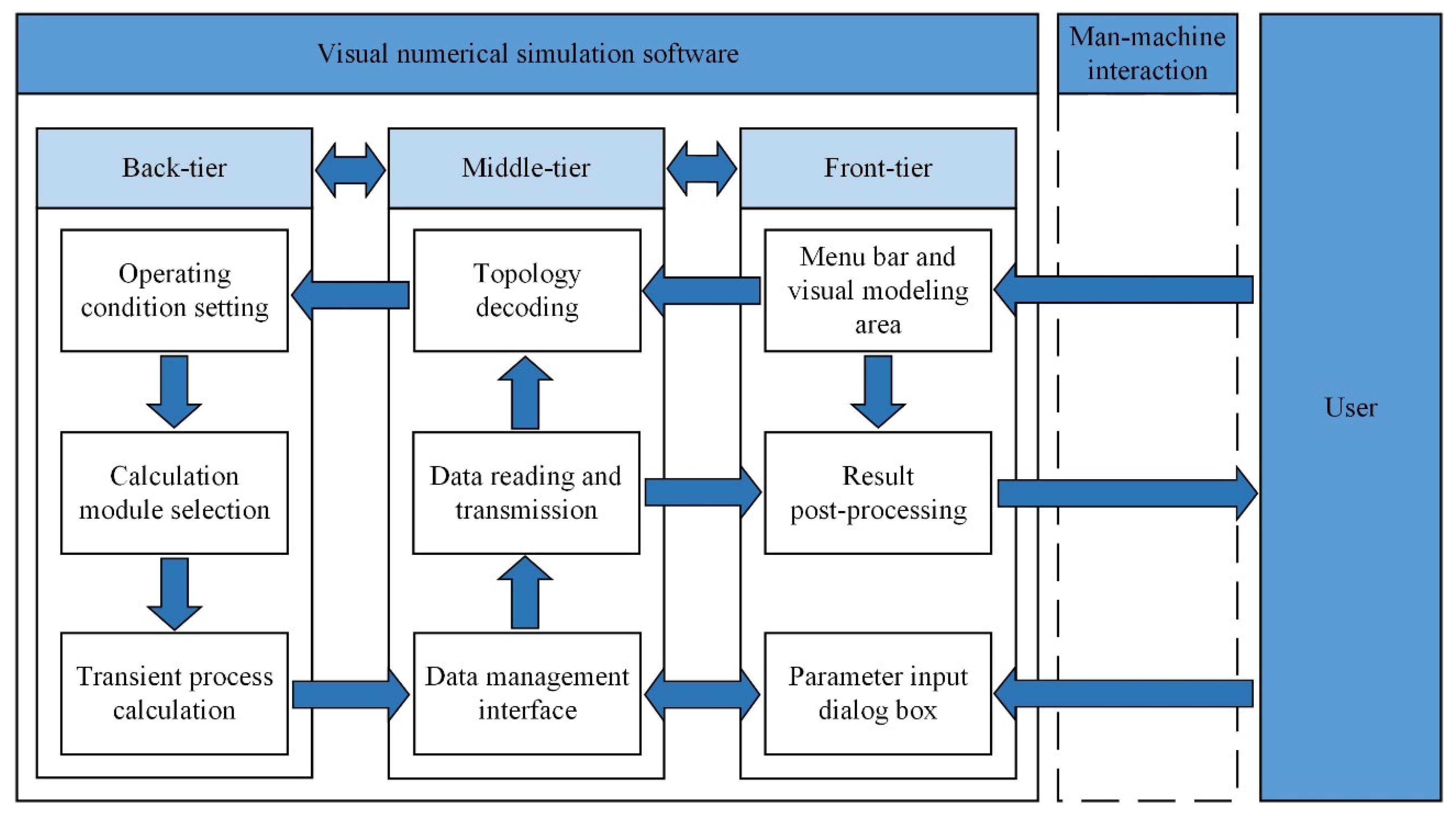
The visual numerical simulation software is designed based on the client/server architecture (C/S architecture). The client realizes the interaction tasks with the user, and the server realizes the management of data. The interfaces and operations of C/S architecture are abundant. The interaction and response speed of C/S architecture are rapid. The user-oriented system design realizes the interactive information service between man and the machine. The software architecture contains three tiers, i.e., back-tier, middle-tier and front-tier. The connotations and relationships of the three tiers of software architecture are shown in Figure 1.

(1) Back-tier

The key of back-tier is the model and the algorithm. The models of the components of the pipeline network system are established. The suitable algorithms are adopted for the solving of models. The models and algorithms are made into general calculation modules. For the numerical simulation for the transient process of the pipeline network system of the water supply project, the operating condition should be set first. Then, under an operating condition, the general calculation modules are selected and called. After the instruction of calculation is input, the calculation of transient process starts and lasts in the set time.

(2) Middle-tier

The key to middle-tier is the decoding and interaction. The topology of pipeline network system is decoded firstly. After the topology decoding, the properties and connected relations of different graphical calculation modules are determined. Then, for different graphical calculation modules, the parameters are input, read and transmitted. The data reading and transmission exist in the back-tier, middle-tier and front-tier. The data management interface realizes the data reading and transmission rapidly and smoothly.

(3) Front-tier

The key to front-tier is the visual interface and pre-post processing. The visual interface of the visual numerical simulation software is integrated in the front-tier. As a general, visual and friendly numerical simulation software, the visual interface is composed of a menu bar, a visual modeling area and a parameter input dialog box. By using the functions of the menu bar, the visual modeling area and the parameter input dialog box, the models and calculation conditions of the pipeline network system can be established and set. After the calculation of the transient process, the post-processing of results is realized in the front-tier. The calculation results of the transient process can be displayed, analyzed and saved.

Under the combination of the three tiers, the visual numerical simulation software can realize the efficient calculation for the transient process of the pipeline network system of the water supply project. The software is developed and integrated in Java. The numerical simulation software contains the following features: professionalization, visualization, generalization, modularization and intellectualization. Specifically,

(1) Professionalization: the models of the pipeline network system are extracted from authoritative literature. The classical algorithms for the calculation of the transient process are adopted. Moreover, several new types of valves and water hammer prevention facilities are considered and included. The transient processes in the water supply network can be simulated in detail, and comprehensively.

(2) Visualization: the software is a user-oriented system to realize the interactive information service between man and a machine. The visual interface of the software integrates all the operating menus and functions. In the visual interface, the model of the pipeline network system is established by graphical modules and interface tools.

(3) Generalization: the application of the software is not limited by the types of the water supply project, the layouts of the pipeline network system or the operating conditions of the transient process. The software is general for the numerical simulation for the transient processes in the water supply network.

(4) Modularization: in software, the models and algorithms are made into general modules. The components of the water supply network, such as pipe, pump and valve, are made into general model modules. The operating conditions of the transient process, such as starting up and shutting down, are made into general calculation modules.

(5) Intellectualization: the software contains several intelligent functions that make the use more convenient and efficient. By importing the CAD file of water supply network, the software can automatically identify the topology of the pipeline network system and then establish the graphical model. The calculation results of the transient process can be output as a formal report. In that report, the calculation results are automatically collected and classified. The changing curves of variables are automatically drawn and inserted.

3. Back-Tier: Model and Algorithm

3.1. Model of Unsteady Flow in Pipelines and Method of Characteristics

The research object of the pipeline network system of the water supply project is the water flow in the pipelines. In the present study, the pipeline network system is the pressure flow and completely filled with water. There is no free water surface in the pipelines. During the transient process, the water flow is unsteady. It is assumed that the water in the pipeline network system is incompressible. The basic equations that describe the unsteady flow in the pipelines contain the momentum equation and continuity equation [5,6]. Those two basic equations are presented in Equation (1).

$$\{\begin{array}{l}\frac{Q}{A}\frac{\partial H}{\partial x}+\frac{\partial H}{\partial t}+\frac{a^2}{gA}\frac{\partial Q}{\partial t}+\frac{a^{2}Q}{gA}\frac{\partial A}{\partial x}-\frac{Q}{A}\sin \theta =0\\ g{A}^2\frac{\partial H}{\partial x}+Q\frac{\partial Q}{\partial x}+A\frac{\partial Q}{\partial t}+\frac{fQ\left|Q\right|}{2D}=0\end{array}$$

(1)

where $Q$ is the discharge in the pipeline, $H$ is the pressure head, $x$ is the distance along the pipeline axis, $D$ is the diameter of the pipeline, $A$ is the cross-sectional area of the pipeline, $\theta$ is the angle between the pipeline axis and horizontal line, $f$ is the Darcy-Weisbach friction coefficient, $a$ is the speed of water hammer wave, $g$ is the acceleration of gravity, $t$ is time.

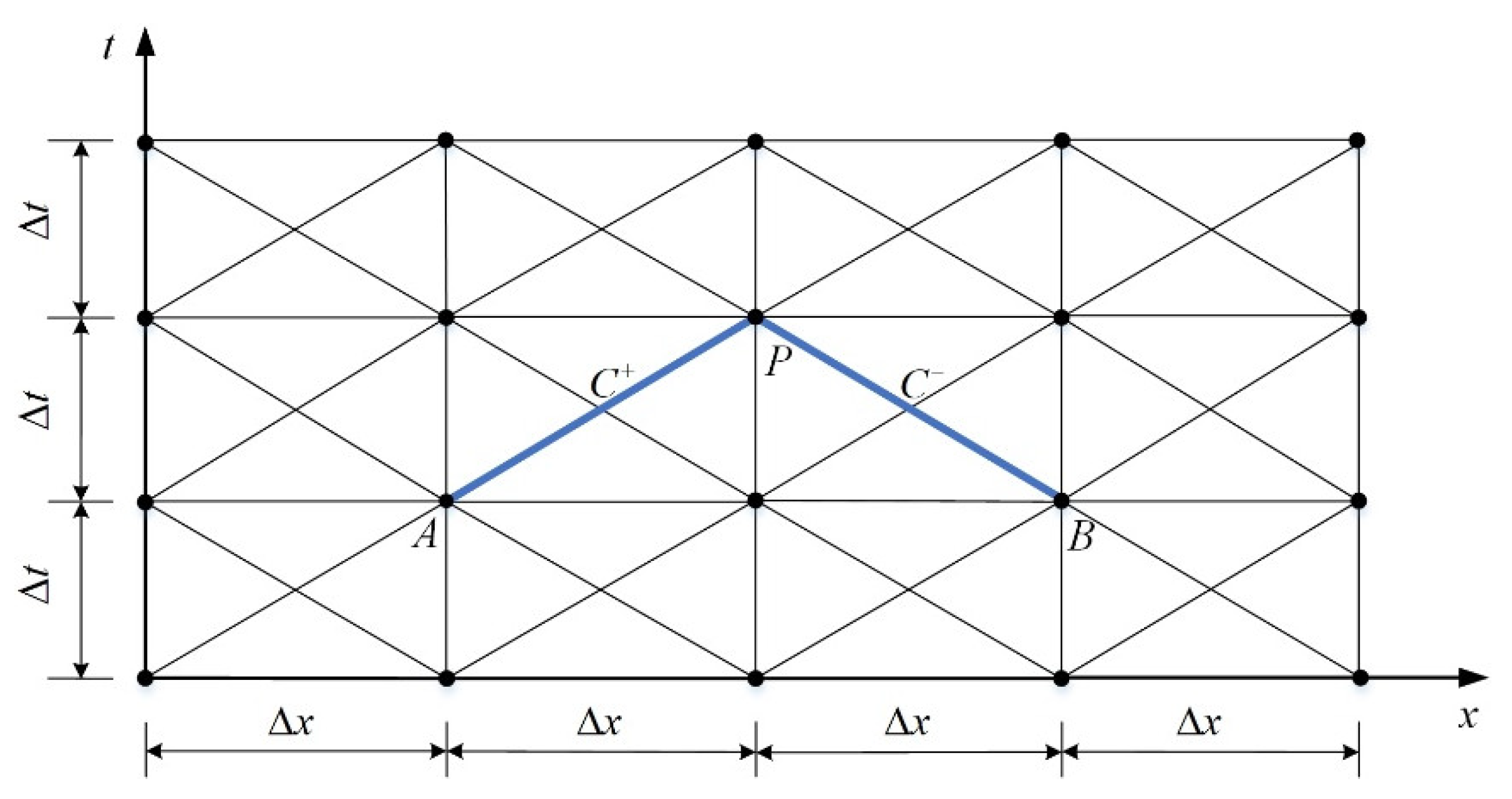
The most widely used method for solving Equation (1) is the method of characteristics [5,6]. The method of characteristics is a kind of one-dimensional numerical solution. By using the integration along the characteristic lines, the ordinary differential equations are transformed into finite difference equations. The finite difference equations are algebraic equations and can be easily solved. The schematic diagram of the method of characteristics for solving Equation (1) is shown in Figure 2.

The abscissa axis of Figure 2 represents the pipeline axis. The pipeline axis is divided into many micro sections with a length of $\Delta x$. The vertical axis of Figure 2 represents the duration time of transient process. $\Delta t$ is the time step of difference calculation. There are two characteristic lines, i.e., $C^{+}$ and $C^{-}$. The characteristic line $C^{+}$ is from point A to point P, the characteristic line $C^{-}$ is from point B to point P.

The equations of characteristic lines are:

$$\{\begin{array}{l}{C}^{+}:\frac{\mathrm{d}x}{\mathrm{d}t}=V+a\approx a\\ C^{-}:\frac{\mathrm{d}x}{\mathrm{d}t}=V-a\approx -a\end{array}$$

(2)

where $V$ is the flow speed in the pipeline.

After the transformation and integration of Equation (1) on Equation (2), the following finite difference equations are obtained.

$$\{\begin{array}{l}{C}^{+}:Q_P=C_{A1}-C_{A2}{H}_P\\ C^{-}:Q_P=C_{B1}+C_{B2}{H}_P\end{array}$$

(3)

where $C_{A1}$ and $C_{A2}$ are the coefficients that are related to the discharge and pressure head of point A, $C_{B1}$ and $C_{B2}$ are the coefficients that are related to the discharge and pressure head of point B.

Based on Equation (3), the discharge and pressure head of point P, i.e., $Q_P$ and $H_P$, can be solved by using the discharges and pressure heads of points A and B. By combining the boundary conditions and initial conditions, the discharges and pressure heads of all cross sections of pipeline network system during the transient process can be solved.

3.2. Models of Other Network Elements

The other elements of pipeline network system of water supply project include pump, valve and water hammer prevention facility. In the present study, the models of other network elements are established by matching with the method of characteristics.

3.2.1. Pump

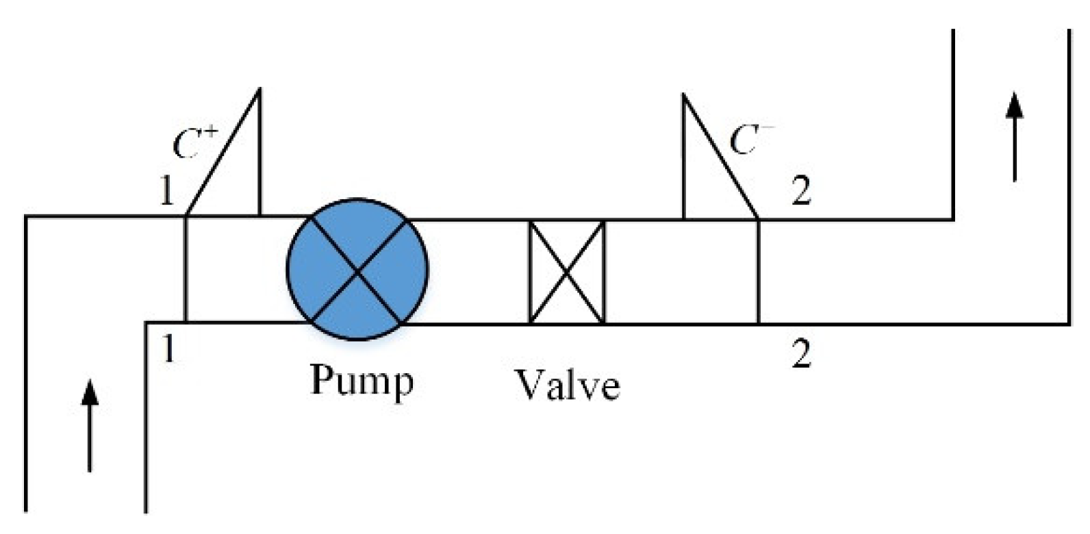
Pump is the pressurized equipment of the pipeline network system of the water supply project [38,39]. There are many kinds of pump. The model of constant speed pump is introduced in the following paragraphs. Figure 3 is the schematic diagram of the constant speed pump.

The model of pump is composed of the pressure head equilibrium equation and inertia equation [5,9]. The pressure head equilibrium equation describes the balance of pressure head between the inlet section of the pump and the output section of the valve. The valve locates at the near right side of pump. The pressure head equilibrium equation of the pump is

$$H=H_{p2}-H_{p1}-H_f$$

(4)

where $H$ is the output head of the pump, $H_{p1}$ and $H_{p2}$ are the pressure head at the inlet section of the pump and the output section of the valve, respectively, $H_f$ is the head loss of the valve.

$H_{p1}$ and $H_{p2}$ can be determined by the following equations of characteristic lines.

$$\{\begin{array}{l}{C}^{+}:H_{P1}=C_{P1}-C_{P2}Q\\ C^{-}:H_{P2}=C_{V1}+C_{V2}Q\end{array}$$

(5)

where $C_{P1}$ and $C_{P2}$ are the coefficients that are related to the discharge and pressure head of the inlet section of the pump, i.e., $Q$ and $H_{P1}$, $C_{V1}$ and $C_{V2}$ are the coefficients that are related to the discharge and pressure head of the output section of the valve, i.e., $Q$ and $H_{P2}$.

$H_f$ can be determined by the following equation [5,9,38,39].

$$H_f=H_{f0}\frac{q\left|q\right|}{{\tau }^2}$$

(6)

where $H_{f0}$ is the head loss of valve when the discharge of the pump is the rated value, i.e., $Q_R$, $\tau =\frac{\theta }{{\theta }_R}$ is the relative opening of the valve, $\theta$ and ${\theta }_R$ are the opening angle and rated opening angle of the valve, respectively, $q=\frac{Q}{Q_R}$ is the relative discharge of the pump.

The inertia equation of the pump is [5,9,38,39]

$${\alpha }_{\Delta t}-\alpha =\frac{\Delta t}{2k}{\beta }_{\Delta t}+\frac{\Delta t}{2k}\left({\alpha }^2+q^2\right)\left[C_0+C_1\left(\pi +\arctan \frac{q}{\alpha }\right)\right]$$

(7)

where $\alpha =\frac{n}{n_R}$ is the relative rotational speed of the pump, $n$ and $n_R$ are the rotational speed and rated rotational speed of the pump, respectively, $\beta =\frac{T}{T_R}$ is the relative torque of the pump, $T$ and $T_R$ are the torque and rated torque of the pump, respectively, the subscript $\Delta t$ represents the value of the variable after $\Delta t$ of the present calculation time, $C_0$ and $C_1$ are the coefficients, $k$ is an intermediate variable.

The models of other kinds of pump, such as variable speed the pump, can be found in [5,9,38,39].

3.2.2. Valve

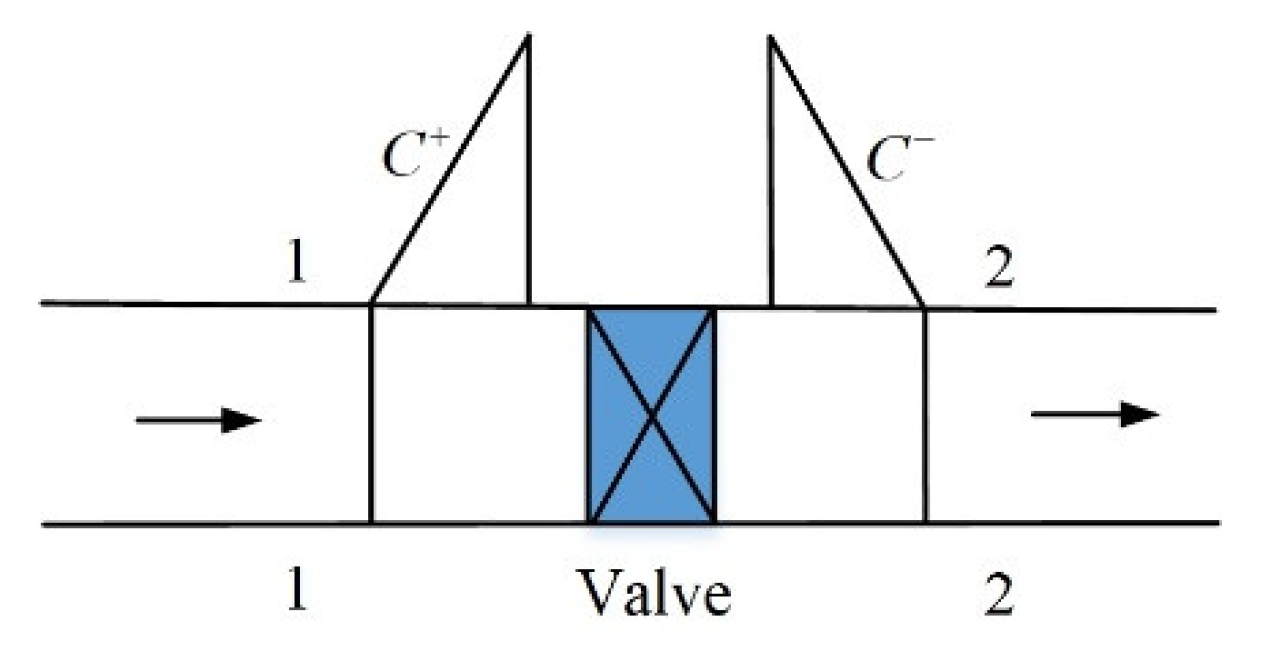
Valve is the discharge regulation equipment of the pipeline network system of the water supply project [9,40]. There are many kinds of valves. The model of gate valve is introduced in the following paragraphs. Figure 4 is the schematic diagram of the gate valve.

The discharge through the valve is [9,40]

$$Q=\mu F\sqrt{2g\Delta H_V}$$

(8)

where $\Delta H_V=H_{V1}-H_{V2}$, $H_{V1}$ and $H_{V2}$ are the pressure head at the inlet section and output section of the valve, respectively, $\mu$ and $F$ are the discharge coefficient and cross-sectional area of the valve when the opening of the valve is $\theta$, respectively.

The relationship among $Q$, $H_{V1}$ and $H_{V2}$ is also determined by the following equations of characteristic lines.

$$\{\begin{array}{l}{C}^{+}:H_{V1}=C_{V1-1}-C_{V1-2}Q\\ C^{-}:H_{V2}=C_{V2-1}+C_{V2-2}Q\end{array}$$

(9)

where $C_{V1-1}$ and $C_{V1-2}$ are the coefficients that are related to the discharge and pressure head of the inlet section of the valve, i.e., $Q$ and $H_{V1}$, $C_{V2-1}$ and $C_{V2-2}$ are the coefficients that are related to the discharge and pressure head of the output section of the valve, i.e., $Q$ and $H_{V2}$.

When the opening of valve is ${\theta }_R$, the discharge through the valve is $Q_R$. Based on Equation (8), $Q_R$ can be expressed as

$$Q_R={\mu }_R{F}_R\sqrt{2g\Delta H_{VR}}$$

(10)

where the subscript $R$ represents the rated value of the variable.

By using Equations (8) and (10), we can get

$$q=c\sqrt{2g\Delta h_V}$$

(11)

where $c=\frac{\mu F}{{\mu }_R{F}_R}$ and $\Delta h_V=\frac{\Delta H_V}{\Delta H_{VR}}$ the subscript $R$ represents the rated value of the variable.

The models of other kinds of the valve, such as regulating valve, hydraulic control valve, air valve, check valve and safety valve can be found in [9,40].

3.2.3. Water Hammer Prevention Facility

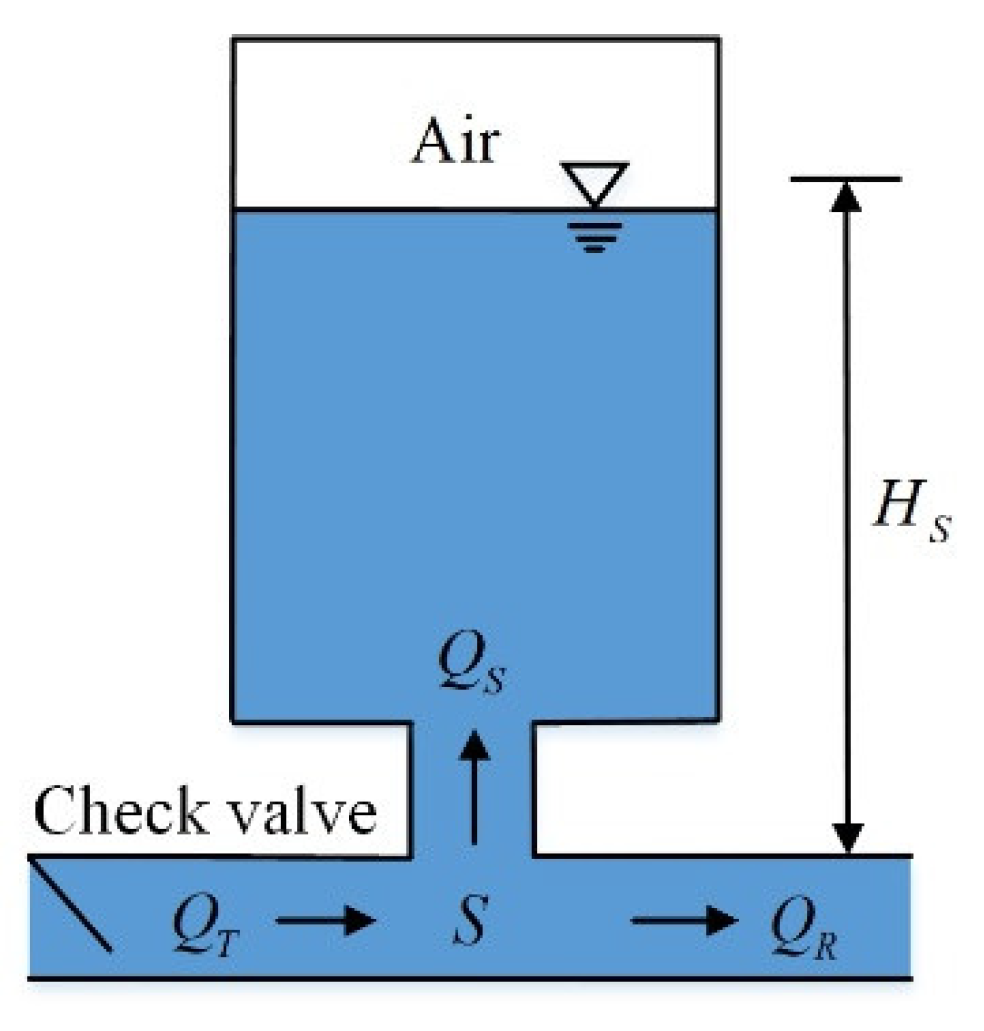
Water hammer prevention facility is the pressure reduction equipment of the pipeline network system of the water supply project [8,9,40]. There are many kinds of water hammer prevention facilities. The model of the air tank is introduced in the following paragraphs. Figure 5 is the schematic diagram of the air tank.

The air in the top of the tank satisfies the following air state equation [8,9,40,41].

$$p{l}^m=C$$

(12)

where $p$ is the pressure of the air in tank, $l$ is the height of the air cushion, $m$ is the polytropic exponent of air and $C$ is the constant.

At the bottom of the air tank, the discharges $Q_T$, $Q_S$ and $Q_R$ satisfies the following continuity equation.

$$Q_T=Q_R+Q_s$$

(13)

where $Q_T$ is the discharge in the pipe before the air tank, $Q_S$ is the discharge that flows into the air tank and $Q_R$ is the discharge in the pipe after the air tank.

The relationship among $Q_S$, $l$ and the water level $H_S$ in air tank is [8,9,40,41]

$$F_A\frac{\mathrm{d}{H}_S}{\mathrm{d}t}=-F_A\frac{\mathrm{d}l}{\mathrm{d}t}=Q_S$$

(14)

The piezometric head at the bottom of the air tank, i.e., point S, is denoted as $H_S^{\ast }$. Then we have

$$H_S^{\ast }=\left(\frac{p}{\gamma }-H_{\Delta }\right)+H_s+{\alpha }_A\left|Q_S\right|Q_S$$

(15)

where $\gamma$ is the unit weight of water, $H_{\Delta }$ is the standard atmospheric pressure and ${\alpha }_A$ is the discharge coefficient of head loss at the throttling orifice of air tank.

The head loss at the bottom of the air tank is neglected. Therefore, we have $H_S=H_T=H_R$. Then the relationship among $H_S$, $Q_T$ and $Q_R$ are determined by the following equations of characteristic lines.

$$\{\begin{array}{l}{C}^{+}:H_S=C_{T1}-C_{T2}{Q}_T\\ C^{-}:H_S=C_{R1}+C_{R2}{Q}_R\end{array}$$

(16)

where $C_{T1}$ and $C_{T2}$ are the coefficients that are related to $Q_T$ and $H_S$, $C_{R1}$ and $C_{R2}$ are the coefficients that are related to $Q_R$ and $H_S$.

The models of other kinds of water hammer prevention facility, such as two-way surge tower and one-way surge tower, can be found in [8,9,40,41].

3.3. Boundary and Initial Conditions

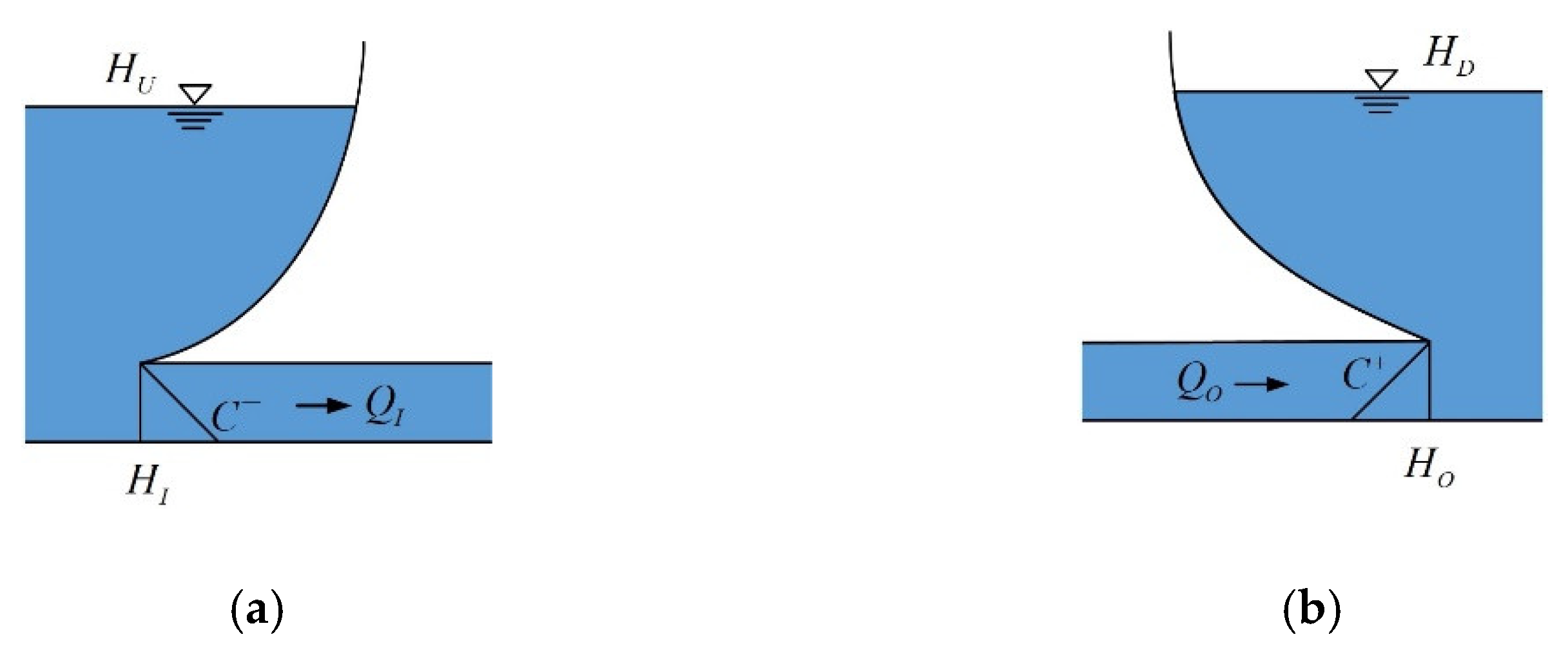
The boundary conditions of pipeline network system of water supply project are the reservoirs, which include upstream reservoir and downstream reservoir [5,6]. The equations of upstream reservoir and downstream reservoir are introduced in the following paragraphs. Figure 6 is the schematic diagram of the upstream reservoir and downstream reservoir.

For the upstream reservoir, the head loss at the water inlet of pipe is neglected. Then we have $H_I=H_U$, in which $H_I$ is the pressure head at the inlet section of pipe and $H_U$ is the water level elevation of upstream reservoir. The relationship between $H_I$ and $Q_I$ is determined by the following equation of characteristic line.

$$C^{-}:H_I=C_{I1}+C_{I2}{Q}_I$$

(17)

where $C_{I1}$ and $C_{I2}$ are the coefficients that are related to $Q_I$ and $H_I$, $Q_I$ is the discharge at the inlet section of pipe.

For the downstream reservoir, the head loss at the water outlet of pipe is neglected. Then we have $H_O=H_D$, in which $H_O$ is the pressure head at the outlet section of pipe, and $H_D$ is the water level elevation of downstream reservoir. The relationship between $H_O$ and $Q_O$ is determined by the following equation of characteristic line.

$$C^{+}:H_O=C_{O1}-C_{O2}{Q}_O$$

(18)

where $C_{O1}$ and $C_{O2}$ are the coefficients that are related to $Q_O$ and $H_O$, $Q_O$ is the discharge at the outlet section of pipe.

The initial conditions are determined by the initial steady state of pipeline network system of water supply project. For an operating condition, the initial state for the calculation of transient process of pipeline network system is set as the steady state. The values of variables under the initial steady state of pipeline network system are the initial conditions for the calculation of transient process.

3.4. Time and Space Discretization

The time and space discretization is about the determination of time step $\Delta t$ and space step $\Delta x$ for the calculation of transient process. Based on the theory of the method of characteristics, the time step $\Delta t$ and space step $\Delta x$ should satisfy the following stability condition [5,6].

$$\Delta t\le \frac{\Delta x}{a}$$

(19)

In the visual numerical simulation software, we take $\Delta t=\frac{\Delta x}{a}$. The time step $\Delta t$ is set and input by the user. In the first stage menu of “Calculation” of the main interface of visual numerical simulation software, there is a second stage menu “Time step”. That menu is specially designed for inputting the time step $\Delta t$ of calculation of transient process. After the input of time step $\Delta t$, the space step $\Delta x$ is calculated automatically in the visual numerical simulation software based on $\Delta x=a\Delta t$. For example, if $a$ is 1000 m/s and the time step $\Delta t$ is set as 0.01 s, the space step $\Delta x$ is 10 m.

4. Middle-Tier: Decoding and Interaction

The task of middle-tier contains the decoding of topology of the pipeline network system and the interaction between the back-tier and the front-tier. The key technological difficulty is the decoding of topology of the pipeline network system, which is illuminated in this section.

The topology decoding is composed of two steps, i.e., automatic encoding and automatic pipeline identification.

4.1. Automatic Encoding

The topology of the pipeline network system is composed of pipelines and nodes. The purpose of automatic encoding is to determine the connection relation between pipelines and nodes. That connection relation should be identified from the graphical model of pipeline network system and expressed by data structure with a specific form. Then the data structure should be transmitted to the computer.

Based on the feature of the topology of pipeline network system, the automatic encoding should realize the following two functions. Firstly, the pipelines and nodes are numbered, respectively. Then, the connection relation among pipelines, upstream nodes and downstream nodes are determined. The automatic encoding is realized by the method of object-oriented programming. The requirements of automatic encoding include:

(a)

All the data structures of encoding are generated by the computer automatically.

(b)

The pipelines and nodes are the basic units. An arbitrary pipeline network system can be described by the pipelines and nodes.

(c)

The encoding can be adjusted dynamically according to the change of graphical model of pipeline network system.

(d)

The data structures of encoding are independent with the data structures of attribute parameters of graphical models.

In the method of object-oriented programming, the pipelines and nodes are regarded as objects. Three data members are added for each object. That data member is called the encoding data member. Among the three data members for an object, the first encoding data member represents the encoding of the object. The second encoding data member represents the upstream connection relation, i.e., the encoding of the upstream pipeline or node of the object. The third encoding data member represents the downstream connection relation, i.e., the encoding of the downstream pipeline or node of the object. Because every object has those three encoding data members, those three encoding data members can be defined in base class.

The encoding is dynamic. The serial number of the object in data structure is regarded as the encoding of the object. With the change of the graphical model of pipeline network system, the serial number of the object in data structure changes accordingly. Then the dynamic encoding is realized. During the calculation of transient process, the data reading and transmission mainly exist in the pipelines, upstream nodes and downstream nodes.

4.2. Automatic Pipeline Identification

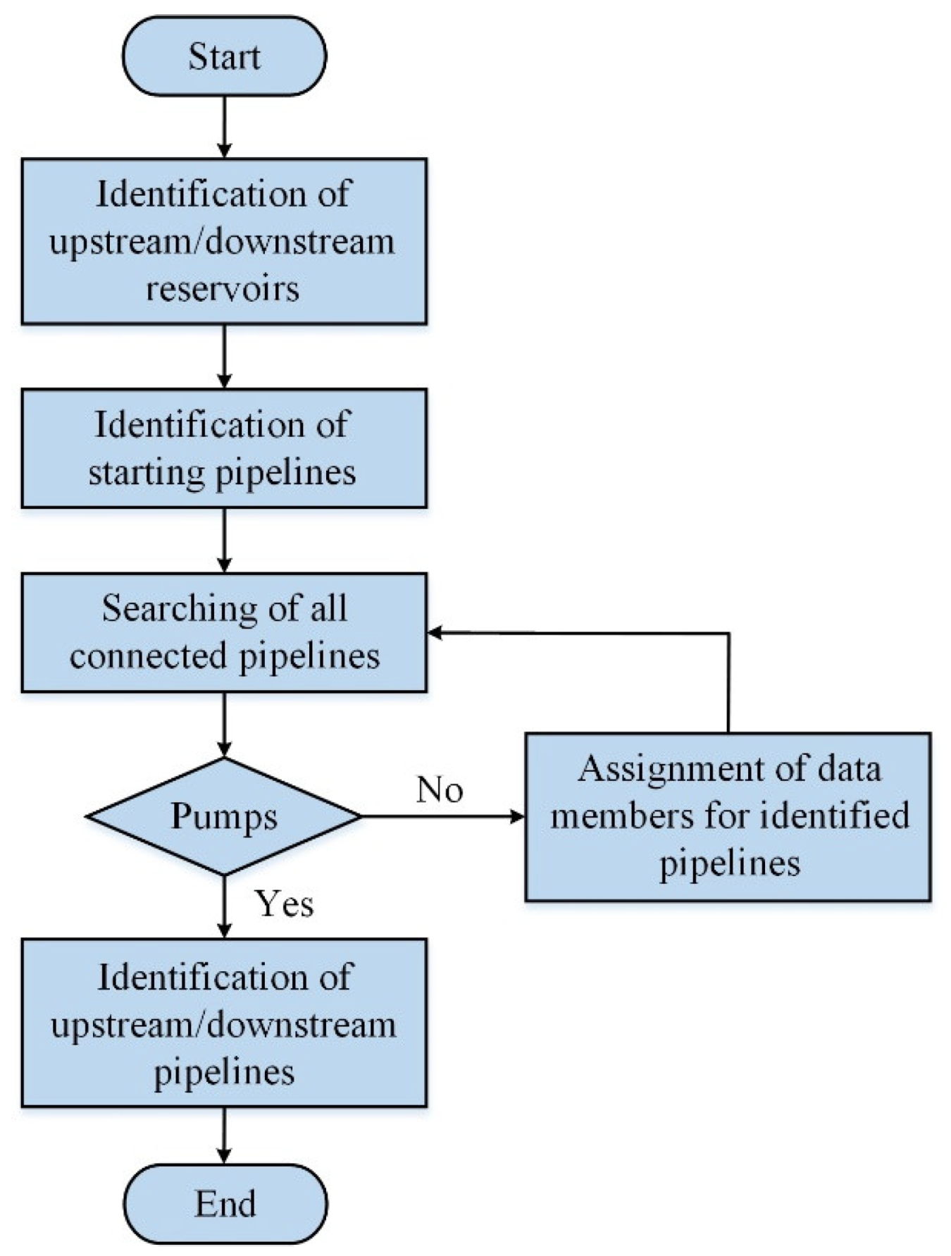
The automatic encoding determines the connection relation between pipelines and nodes. Based on the result of automatic encoding, the automatic pipeline identification aims to arrange the pipelines and nodes in the order from upstream to downstream. All the pipelines are divided into two parts, i.e., upstream pipelines and downstream pipelines.

In order to realize the function of automatic pipeline identification, two data members are added for each pipeline. For a pipeline, the first data member is used to store the information of its upstream pipeline, and the second data member is used to store the information of its downstream pipeline. The automatic pipeline identification contains two aspects.

Aspect 1—from upstream to downstream: in the process of automatic pipeline identification, the pipelines connected with upstream reservoir are identified firstly. Those pipelines are denoted as the starting pipelines. According to the starting pipelines, the searching is carried out along pipelines from upstream to downstream. For a pipeline, all the connected pipelines are identified. The searching stops when the upstream pipeline connected with pump is identified.

Aspect 2—from downstream to upstream: in the process of automatic pipeline identification, the pipelines connected with downstream reservoir are identified firstly. Those pipelines are denoted as the starting pipelines. According to the starting pipelines, the searching is carried out along pipelines from downstream to upstream. For a pipeline, all the connected pipelines are identified. The searching stops when the downstream pipeline connected with pump is identified.

The procedure of automatic pipeline identification is shown in Figure 7.

5. Front-Tier: Visual Interface and Pre-Post Processing

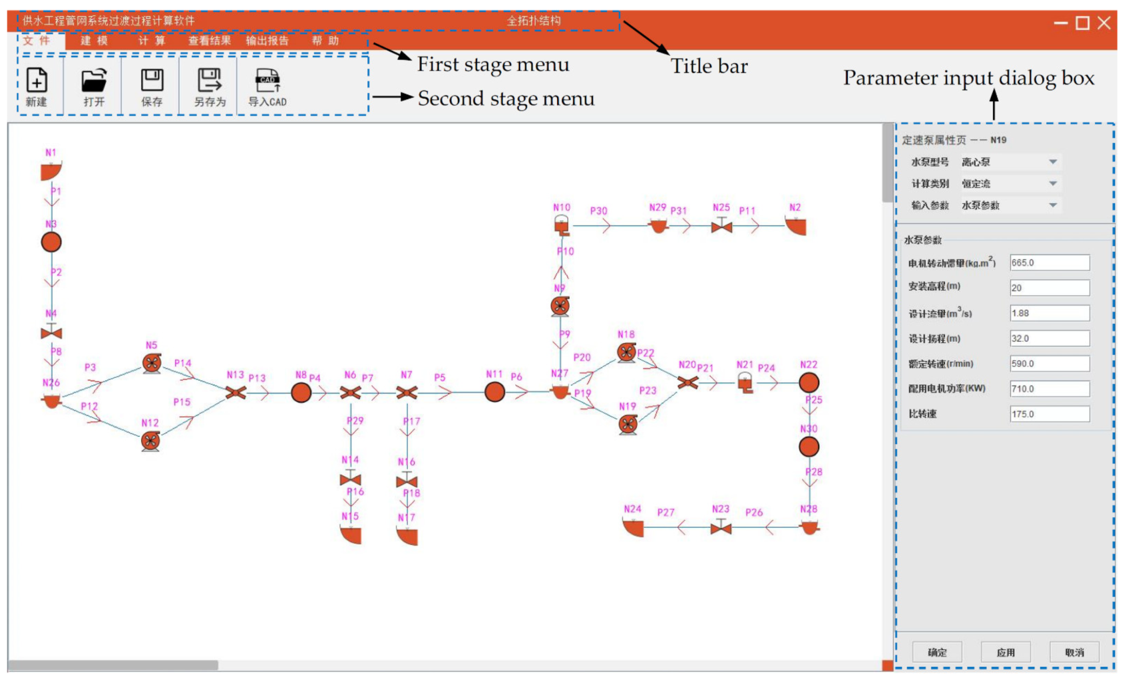
Following the principles of practicability, concision, beauty and friendly man–machine interaction, the main interface of visual numerical simulation software for transient process of pipeline network system of water supply project is designed as Figure 8.

The main interface includes three parts, i.e., menu bar, visual modeling area and parameter input dialog box. The main functions and modules are included in the menu bar. The visual modeling area is used to achieve the graphical modeling of pipeline network system. The practical and three-dimensional pipeline network system of the water supply project is converted into two-dimensional topology. The topology is composed of general modules. The parameter input dialog box is used to input the attribute parameters of modules. The operating condition is also set in the parameter input dialog box.

The main functions and modules are emphatically introduce based on the design of the menu bar in the following paragraphs. The two-stage menus are designed for the menu bar. The first stage menu contains six items, i.e., file, modeling, calculation, result view, report output and help. The functions of six items of the first stage menu are shown in

Table 1. Functions of six items of the first stage menu.

Items of the First Stage Menu	Functions
File	Create new project, open, save and save as project, import CAD file.
Modeling	Establish graphical model by using general modules, deal and check the graphical model.
Calculation	Set the calculation parameters and conditions, start the calculation of transient process, save the calculation results.
Result view	View, draw and analyze the calculation results of transient process.
Report output	Output the calculation results of transient process as a formal report.
Help	Introduce the functions of software, provide the tutorial.

.

The detailed items and functions of the second stage menu are presented in

Table 2. Detailed items and functions of the second stage menu.

Items of the First Stage Menu	Items of the Second Stage Menu	Functions
File	New	Establish a new project
	Open	Open an existed project
	Save	Save current project
	Save as	Change storage path of current project and then save it
	Import CAD	Import CAD file
Modeling	Upstream reservoir	General module, draw model of upstream reservoir in visual modeling area
	Downstream reservoir	General module, draw model of downstream reservoir in visual modeling area
	Middle reservoir	General module, draw model of middle reservoir in visual modeling area
	Constant speed pump	General module, draw model of constant speed pump in visual modeling area
	Variable speed pump	General module, draw model of variable speed pump in visual modeling area
	One-way surge tower	General module, draw model of one-way surge tower in visual modeling area
	Two-way surge tower	General module, draw model of two-way surge tower in visual modeling area
	Air tank	General module, draw model of air tank in visual modeling area
	Pipeline	General module, draw model of pipeline in visual modeling area
	Free end	General module, draw model of free end in visual modeling area
	Node	General module, draw model of node in visual modeling area
	Bifurcated point	General module, draw model of bifurcated point in visual modeling area
	Gate valve	General module, draw model of gate valve in visual modeling area
	Regulating valve	General module, draw model of regulating valve in visual modeling area
	Hydraulic control valve	General module, draw model of hydraulic control valve in visual modeling area
	Air valve	General module, draw model of air valve in visual modeling area
	Check valve	General module, draw model of check valve in visual modeling area
	Safety valve	General module, draw model of safety valve in visual modeling area
	Water hammer prevention valve	General module, draw model of water hammer prevention valve in visual modeling area
	Undo	Undo operation in previous step
	Recovery	Recovery revocation operation in previous step
	Zoom in	Zoom in graphical modeling in visual modeling area
	Zoom out	Zoom out graphical modeling in visual modeling area
	Clear drawing board	Delete all graphical models in visual modeling area
	Batch input	Input parameters of a kind in batches
	Select all	Select all graphical models in visual modeling area
	Check pipeline	Check the connection between pipelines and nodes
	Vertical alignment	Realize vertical alignment of selected nodes
	Horizontal alignment	Realize horizontal alignment of selected nodes
Calculation	Calculation time	Input calculation time of transient process
	Time step	Input time step of calculation of transient process
	Output interval	Input time interval of result output
	Iteration accuracy of head	Input iteration accuracy of head for calculation of steady flow
	Iteration accuracy of discharge	Input iteration accuracy of discharge for calculation of steady flow
	Start calculation	Start the calculation of transient process
Result view	Results list of steady flow	View calculation results of steady flow
	Results list of unsteady flow	View calculation results of unsteady flow and then draw
	Extrema list of unsteady flow	View extrema of calculation results of unsteady flow
Report output	Screen capture	Realize screen capture of visual modeling area
	Report output	Output calculation results of transient process as a formal report
	Print report	Print report in different document formats
Help	About software	Introduce development information of software
	Function introduction	Introduce functions of software

.

After the graphical model of the pipeline network system is established, the attribute parameters of models can be input based on the general modules. By double clicking a module, the parameter input dialog box pops up. For different modules, the different attribute parameters are needed. After the input of attribute parameters, the parameters are saved in modules and can be called for the calculation of the transient process.

The characteristic curves of pump are input in the module of pump. Two methods for the input of characteristic curves of pump are provided in the software. The first method is the manual input of characteristic curves. The user prepares the file of characteristic curves of pump in the format of Excel. Then by inputting the file into the pump module, the characteristic curves of discharge and characteristic curves of moment can be presented in the software. The second method is the automatic generation of characteristic curves. A database of the characteristic curves of pump is embedded in the software. For a pump, the characteristic curves can be obtained from the database based on its specific speed and curve interpolation.

6. Engineering Examples

After the combination of back-tier, middle-tier and front-tier, the visual numerical simulation software can realize the efficient calculation for transient process of pipeline network system of water supply project. For a pipeline network system, the procedure of the calculation for transient process by using the software includes the following three steps.

Step 1:

The actual layout of pipeline network system is divided into several pipelines and nodes. Then the pipeline network system can be abstracted into a two-dimensional topology. Based on the topology, the graphical model of pipeline network system is established in visual modeling area by using the general modules. For all the modules, the attribute parameters are input. As a result, a complete graphical model of pipeline network system is obtained. The graphical model reflects the layout, structure and characteristic of pipeline network system.

Step 2:

The operating condition is set in the modules of pumps and valves. The calculation parameters and conditions are set in the first stage menu of calculation. After all the parameters of operating condition and calculation conditions are set, the calculation of transient process can start.

Step 3:

After the calculation of transient process, the results can be saved in the format of Excel. The results of steady flow and unsteady flow can be viewed in the software directly. The changing curves of variables can be drawn based on the calculation results of unsteady flow. According to the results and curves, the characteristics of transient process of pipeline network system can be analyzed and evaluated. The calculation results of transient process can also be output as a formal report.

In the following parts of this section, two engineering examples, i.e., pipeline network system of pressure flow without pump and pipeline network system of pressure flow with pump, are selected to illustrate the practical application of software and verify the accuracy of calculation results. Both of those two pipeline network systems are pressure flow, and there is no free water surface in the pipelines. The two engineering examples are actual water supply projects. The calculation results of the present software are compared with those of one existing software, i.e., HAMMER [33,34].

HAMMER is a widely used commercial software for the numerical simulation for transient process of pipeline network system of water supply project. The modeling theory and method of HAMMER are the same with those of the present software. Moreover, the solution method of HAMMER is also the method of characteristics. However, for the treatment of many technical and programming details, the two kinds of software are different. For example,

(1) For the calculation of transient process, the characteristic curves of pump and valve need to be interpolated because the data points of original characteristic curves are very limited. In the present software, the interpolation of characteristic curves is realized by the method of Lagrange interpolation. However, the interpolation method of HAMMER is not public. Therefore, the interpolation methods of characteristic curves of pump and valve for the two kinds of software cannot keep the same.

(2) For the calculation of transient process, the equations of pump should be solved together with the equations of pipelines based on iteration. In the present software, the iteration solution is realized by the method of Newton-Raphson iteration. However, the iteration method of HAMMER is not public. Therefore, the iteration methods and accuracies of equations of pump and pipelines for the two kinds of software cannot keep the same.

The present software and HAMMER are large and complex. Besides the basic models, solution methods and initial conditions, there are lots of technical and programming details that would lead to the calculation deviations between the two kinds of software. Because many technical and programming details of HAMMER are not public, it is difficult to make all the calculation conditions of the two kinds of software the same. The calculation deviations between the two kinds of software are difficult to avoid. As a new software, the calculation results of the present software remain to be tested. As a widely used commercial software, the calculation results of HAMMER are credible and can be regarded as a reference. Hence, in order to verify the rationality of treatment of details and accuracy of calculation results of the present software, the contrastive analysis is necessary.

6.1. Pipeline Network System of Pressure Flow without Pump

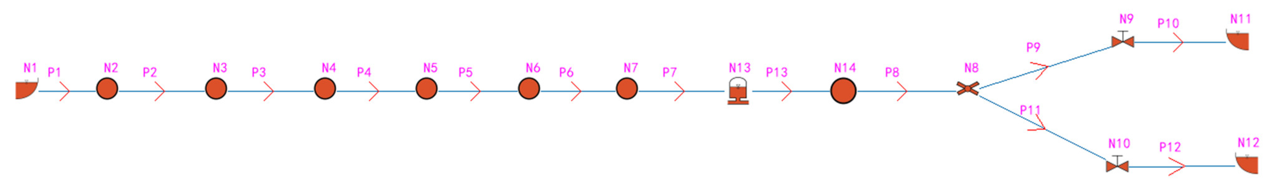
The pipeline network system of pressure flow without pump selected in this section is designed for water transfer. From the upstream reservoir to downstream reservoir, the length of the whole pipeline is about 71.07 km. At the end of the pipeline network system, two regulating valves are set in parallel. One regulating valve is used for normal operation, and the other regulating valve is used for emergency reserve. According to the actual layout of pipeline network system of pressure flow without pump, the graphical model of pipeline network system is established by present software and shown in Figure 9.

In Figure 9, N1 is the upstream reservoir, N11 and N12 are the downstream reservoirs. P1–P13 are the pipelines. N2–N7 and N14 are the tandem nodes. N9 and N10 are the two regulating valves. N8 is the bifurcated point. N13 is the two-way surge tower. The values of parameters of pipelines are shown in

Table 3. Values of parameters of pipelines for the selected pipeline network system of pressure flow without pump.

Pipelines	Length (m)	Diameter (m)	Speed of Water Hammer Wave (m/s)	Roughness Coefficient
P1	25,162.00	3.16	1000	0.014
P2	6011.00	2.20	1000	0.012
P3	30,468.00	3.16	1000	0.014
P4	3714.00	2.20	1000	0.012
P5	3468.00	3.16	1000	0.014
P6	1393.00	2.20	1000	0.012
P7	466.00	3.16	1000	0.014
P13	269.00	3.16	1000	0.014
P8	83.15	2.20	1000	0.012
P9	20.50	1.56	1000	0.012
P10	15.00	1.56	1000	0.012
P11	20.50	1.56	1000	0.012
P12	15.00	1.56	1000	0.012

.

Four operating conditions are selected for the calculation and comparison. The information of the four operating conditions is shown in

Table 4. Four operating conditions for the selected pipeline network system of pressure flow without pump.

Operating Conditions	Water Level of Upstream Reservoir (m)	Water Level of Downstream Reservoir (m)	Discharge of Water Transfer (m3/s)	Movement of Regulating Valves
GF1	87.17	12.45	7.64	N9 shuts down linearly from rated opening to zero opening in 100 s, N10 stays shut.
GF2	87.17	12.45	7.64	N9 and N10 shut down linearly from rated opening to zero opening in 61 s simultaneously.
GF3	69.20	12.45	7.64	N9 opens linearly from zero opening to rated opening in 50 s, N10 stays shut.
GF4	69.20	12.45	7.64	N9 and N10 open linearly from zero opening to rated opening in 50 s simultaneously.

.

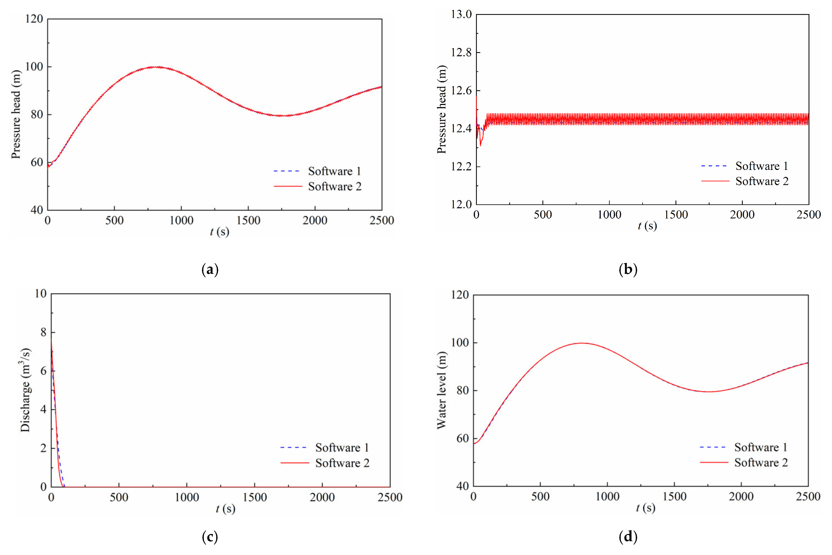
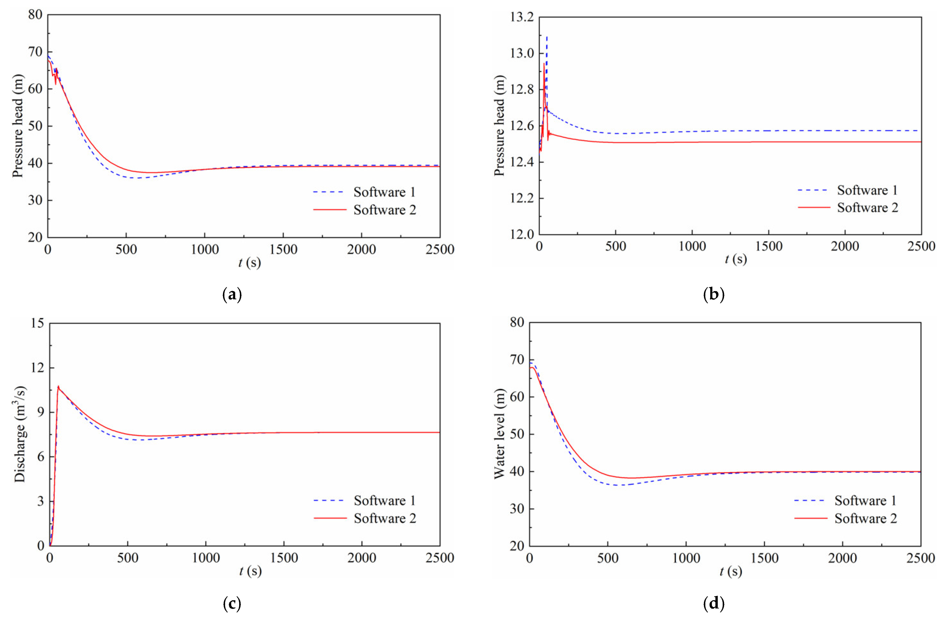
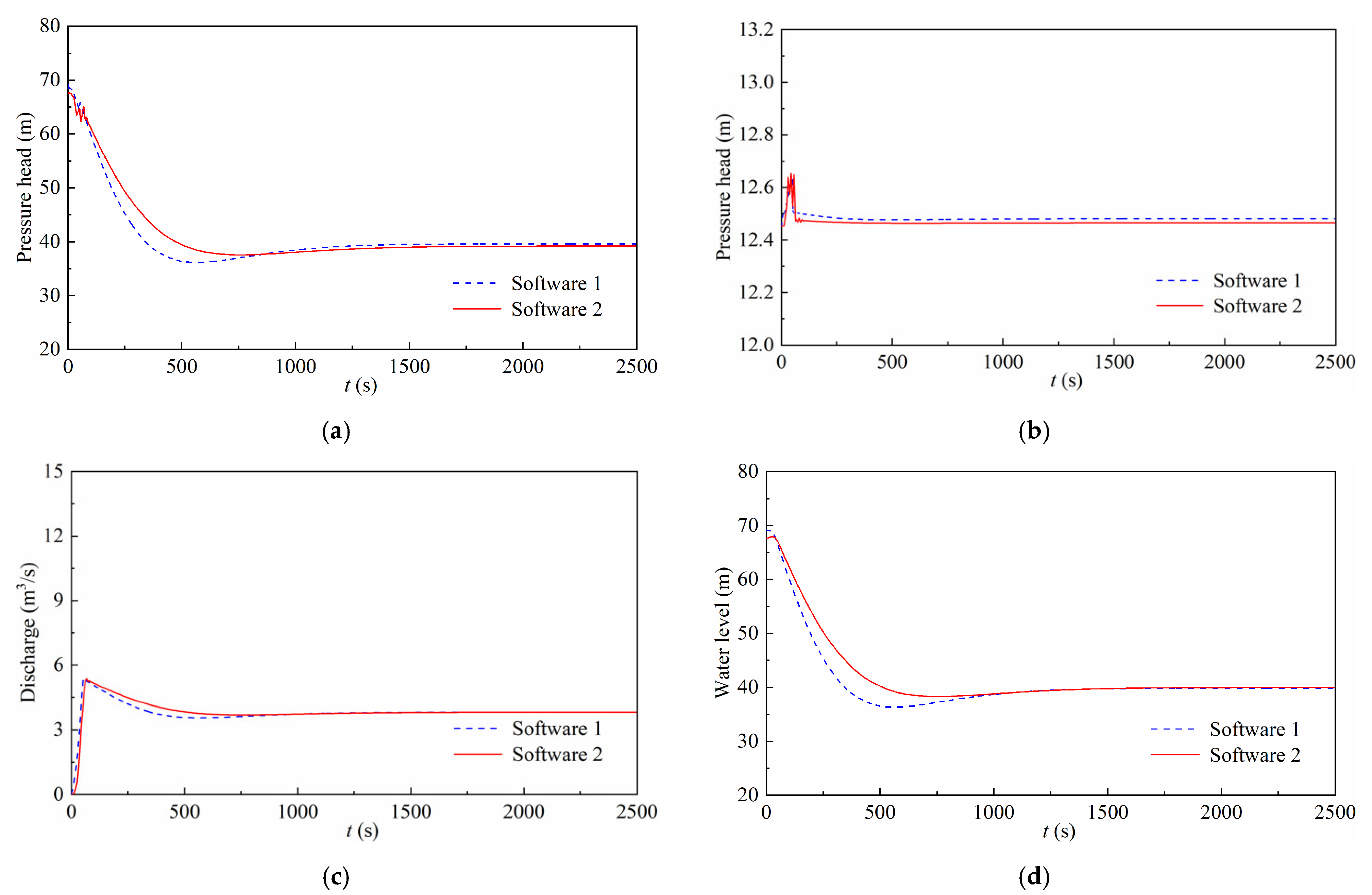
Under the four operating conditions in Table 4, the transient process for the selected pipeline network system of the pressure flow without the pump can be calculated by using the present software and the HAMMER. For each operating condition, four variables, i.e., pressure head at the inlet section of valve, pressure head at the output section of valve, discharge through the valve and water level in the two-way surge tower are presented and compared. The comparisons of calculation results under GF1, GF2, GF3 and GF4 are shown in Figure 10, Figure 11, Figure 12 and Figure 13, respectively. Software 1 represents the present software and software 2 represents the HAMMER.

Figure 10, Figure 11, Figure 12 and Figure 13 show that:

(1) For the transient processes of the four variables under the four operating conditions, the change laws of calculation results of software 1 are consistent with those of software 2. Therefore, the physical laws reflected from the calculation results of software 1 are correct.

(2) Under the four operating conditions, the maximum relative error of the extremum of pressure head at the inlet section of valve is 3.68% and occurs in GF4. The maximum relative error of the extremum of pressure head at the output section of valve is 4.98% and occurs in GF3. The maximum relative error of the extremum of water level in the two-way surge tower is 4.99% and occurs in GF4. The above results indicate that the errors of calculation results between software 1 and software 2 are small. Therefore, the calculation results of software 1 are accurate.

To sum up, the software 1 can calculate the transient process for the pipeline network system of pressure flow without pump reasonably and accurately.

6.2. Pipeline Network System of Pressure Flow with Pump

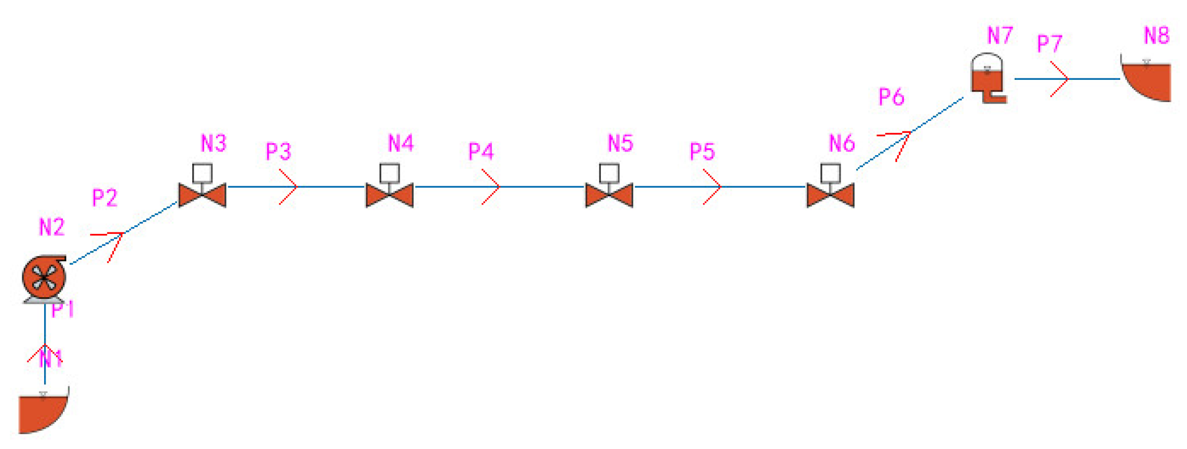
The pipeline network system of pressure flow with pump selected in this section is designed for water supplement of reservoir. The length of the whole pipeline is about 2.65 km. The water supplement from downstream reservoir to upstream reservoir is realized by one pump. According to the actual layout of pipeline network system of pressure flow with pump, the graphical model of pipeline network system is established by present software and shown in Figure 14.

In Figure 14, N1 is the downstream reservoir, and N8 is the upstream reservoir. P1-P7 are the pipelines. N2 is the pump. N3–N6 are the air valves. N7 is the one-way surge tower. The values of parameters of pipelines are shown in

Table 5. Values of parameters of pipelines for the selected pipeline network system of pressure flow with pump.

Pipelines	Length (m)	Diameter (m)	Speed of Water Hammer Wave (m/s)	Roughness Coefficient
P1	18.14	0.90	1000	0.012
P2	30.00	0.90	1000	0.012
P3	701.00	0.90	1000	0.012
P4	536.00	0.90	1000	0.012
P5	344.00	0.90	1000	0.012
P6	30.00	0.90	1000	0.012
P7	989.27	0.90	1000	0.012

.

The basic data of the pump are shown in

Table 6. Basic data of the pump.

Parameters	Values
Rated discharge (m3/s)	0.67
Rated lift (m)	59.00
Rated rotational speed (r/min)	991.00
Specific speed	98.00

.

Three operating conditions are selected for calculation and comparison. The information of the three operating conditions is shown in

Table 7. Three operating conditions for the selected pipeline network system of pressure flow with the pump.

Operating Conditions	Water Level of Downstream Reservoir (m)	Water Level of Upstream Reservoir (m)	Pump Lift (m)	Movement of Regulating Valves
PF1	6.70	59.15	Rated lift	Pump power-off, N3 shuts down linearly from rated opening to zero opening in 6 s.
PF2	7.70	59.15	Minimum lift	Pump power-off, N3 shuts down linearly from rated opening to zero opening in 6 s.
PF3	5.70	59.15	Maximum lift	Pump power-off, N3 shuts down linearly from rated opening to zero opening in 6 s.

.

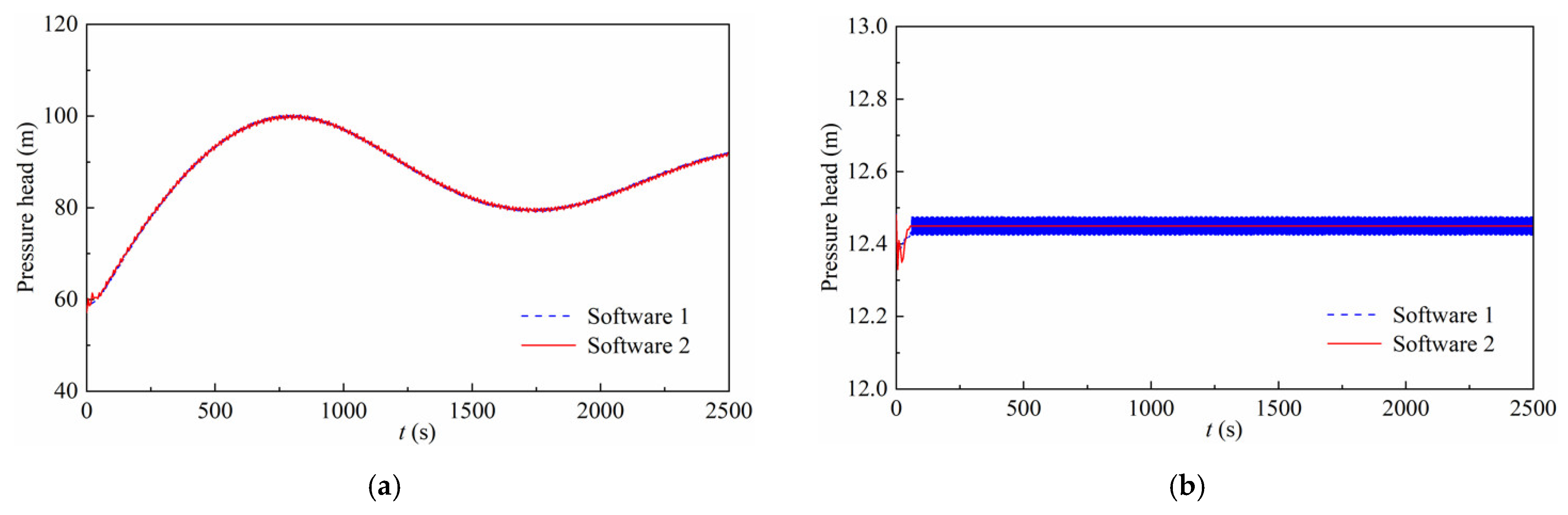
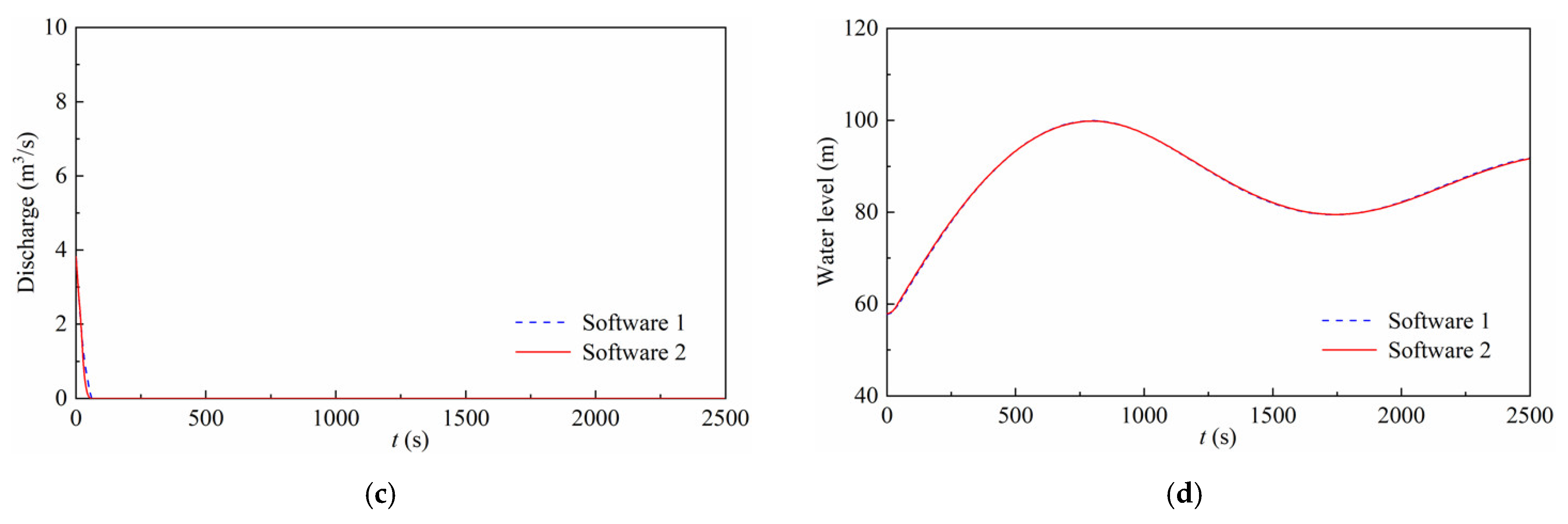
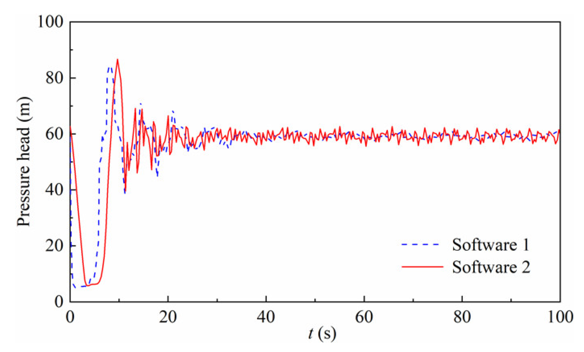
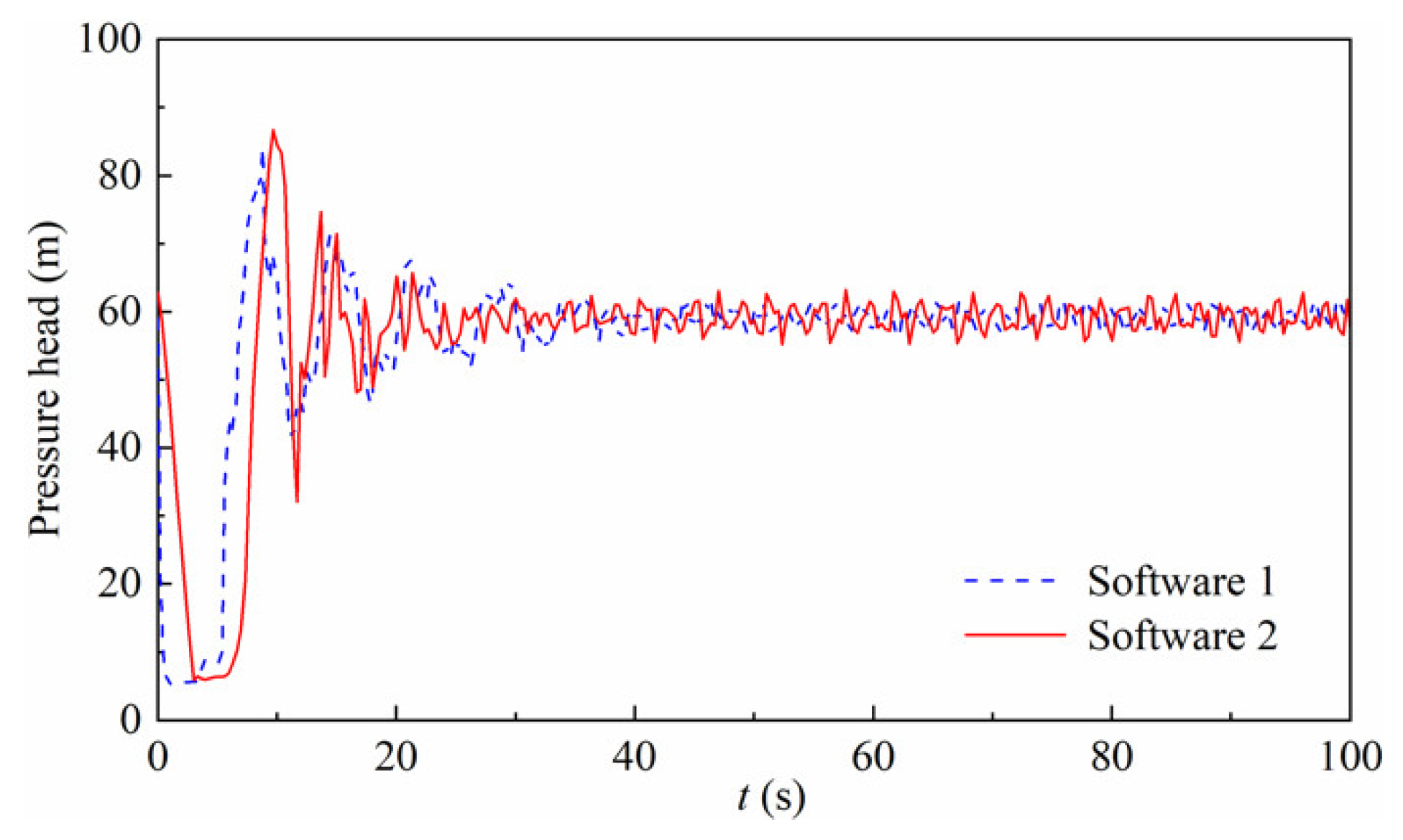
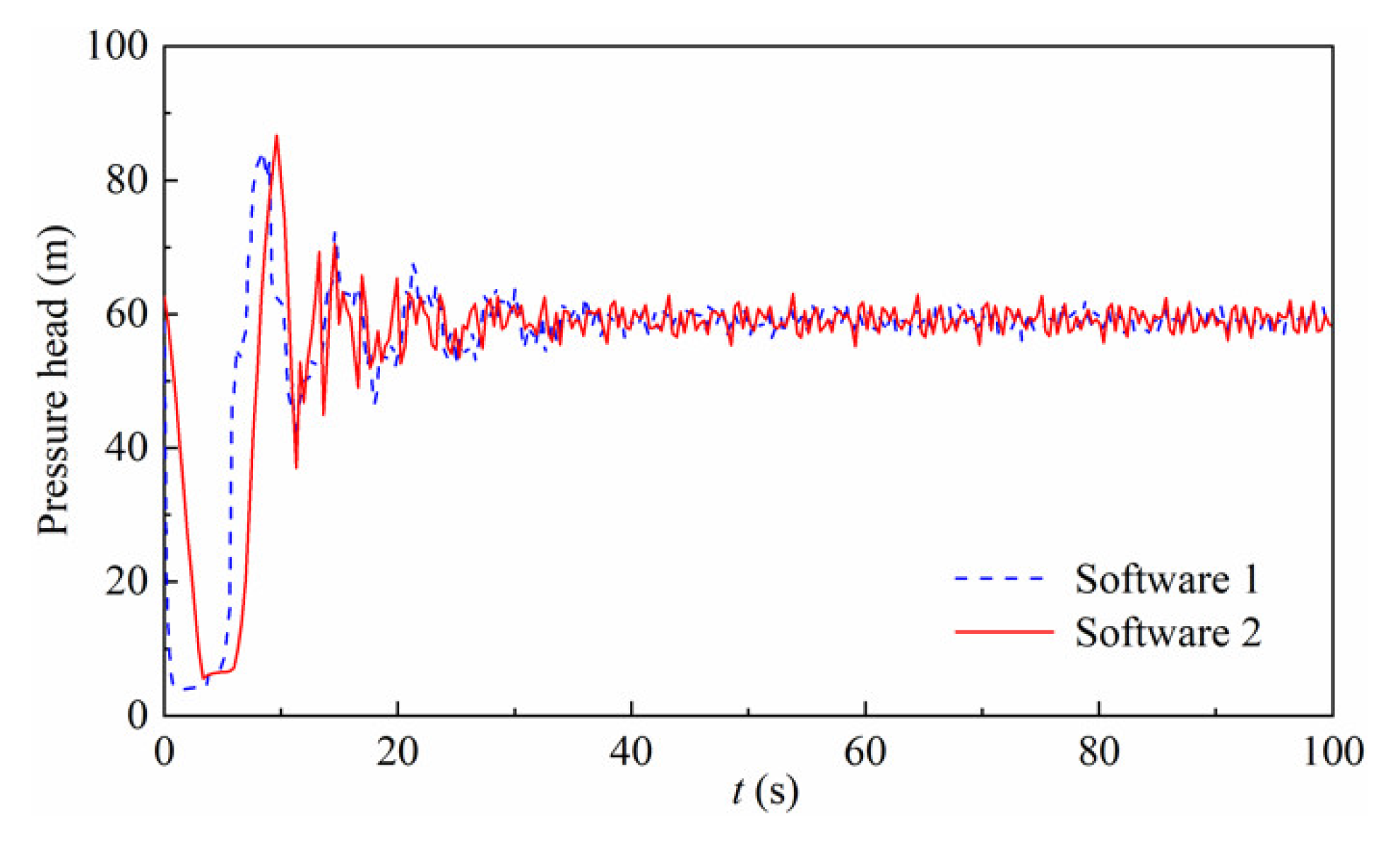
Under the three operating conditions in Table 7, the transient process for the selected pipeline network system of pressure flow with pump can be calculated by using the present software and the HAMMER. For each operating condition, one variable, i.e., pressure head at the output section of valve N3, is presented and compared. The comparisons of calculation results under PF1, PF2 and PF3 are shown in Figure 15, Figure 16 and Figure 17, respectively. Software 1 represents the present software, and software 2 represents the HAMMER.

Figure 15, Figure 16 and Figure 17 show that:

(1) For the transient processes of the pressure head at the output section of valve N3 under the three operating conditions, the change laws of calculation results of software 1 are consistent with those of software 2. Therefore, the physical laws reflected from the calculation results of software 1 are correct.

(2) Under the three operating conditions of PF1, PF2 and PF3, the maximum relative errors of the extremum of pressure head at the output section of valve N3 are 2.41%, 2.02% and 2.60%, respectively. The above results indicate that the errors of calculation results between software 1 and software 2 are small. Therefore, the calculation results of software 1 are accurate.

To sum up, the software 1 can calculate the transient process for the pipeline network system of pressure flow with pump reasonably and accurately.

7. Summary and Conclusions

The visual numerical simulation software for transient process of the pipeline network system of the water supply project is studied and developed. The practical application of software is illustrated, and the accuracy of calculation results is verified. The conclusions are:

(1) The visual numerical simulation software is designed based on the C/S architecture. The software architecture contains three tiers, i.e., back-tier, middle-tier and front-tier. Under the combination of the three tiers, the visual numerical simulation software can realize the efficient calculation for transient process of pipeline network system of water supply project. The numerical simulation software contains the following features: professionalization, visualization, generalization, modularization and intellectualization.

(2) The method for solving the basic equations of unsteady flow in the pipelines is the method of characteristics. The boundary conditions of pipeline network system of water supply project include pump, valve, water hammer prevention facility and reservoir. The task of middle-tier contains the decoding of topology of pipeline network system and the interaction between back-tier and front-tier. The topology decoding is composed of two steps, i.e., automatic encoding and automatic pipeline identification. The main interface includes three parts, i.e., menu bar, visual modeling area and parameter input dialog box.

(3) The visual numerical simulation software can calculate the transient process for the pipeline network system of both pressure flow without pump and pressure flow with pump reasonably and accurately. The physical laws reflected from the calculation results of software are correct. The calculation results of software are accurate.

The following points should be noted:

(1) In the current version of software, the texts and words of the visual interface are in Chinese. An English version will be updated in the future.

(2) At present, the visual numerical simulation software is developed and used by the authors and their teams. The ranges of application of the software include scientific research, technology consulting, and engineering design. The software is not open source. In near future, we aim to promote it to be a commercial software and available for the general public.

(3) As space is limited, only two engineering examples are presented and one existing software, i.e., HAMMER, is compared. The calculation results of software are not compared with the measured data because the measured data for transient process of pipeline network system of water supply project are scarce.

(4) In the visual numerical simulation software, there is not a special module for flowmeter. If the flowmeter has no influence on the flow state of water in the pipeline and has no head loss, such as electromagnetic flowmeter and ultrasonic flowmeter, the flowmeter can be equivalently regarded as a part of pipeline and then simulated in the software. If the flowmeter has head loss, such as differential pressure flowmeter and thermal time of flight flow meter [42], the flowmeter cannot be simulated in the software.

References

- Twort, A.C.; Ratnayaka, D.D.; Brandt, M.J. Water Supply; Elsevier: Amsterdam, The Netherlands, 2000. [Google Scholar]
- McGhee, T.J.; Steel, E.W. Water Supply and Sewerage; McGraw-Hill: New York, NY, USA, 1991. [Google Scholar]
- Rangwala, S.C.; Rangwala, K.S.; Rangwala, P.S. Water Supply and Sanitary Engineering; Charotar Publishing House: Gujarat, India, 2005. [Google Scholar]
- Swamee, P.K.; Sharma, A.K. Design of Water Supply Pipe Networks; John Wiley & Sons: Hoboken, NJ, USA, 2008. [Google Scholar]
- Chaudhry, M.H. Applied Hydraulic Transients; Springer: New York, NY, USA, 2014. [Google Scholar]
- Wylie, E.B.; Streeter, V.L.; Suo, L.S. Fluid Transients in Systems; Prentice Hall: Englewood Cliffs, NJ, USA, 1993. [Google Scholar]
- Boulos, P.F.; Karney, B.W.; Wood, D.J.; Lingireddy, S. Hydraulic transient guidelines for protecting water distribution systems. J. Am. Water Work. Assoc. 2005, 97, 111–124. [Google Scholar] [CrossRef]
- Larock, B.E.; Jeppson, R.W.; Watters, G.Z. Hydraulics of Pipeline Systems; CRC Press: Boca Raton, FL, USA, 1999. [Google Scholar]
- Tullis, J.P. Hydraulics of Pipelines: Pumps, Valves, Cavitation, Transients; John Wiley & Sons: Hoboken, NJ, USA, 1989. [Google Scholar]
- Guo, W.C.; Zhu, D.Y. A review of the transient process and control for a hydropower station with a super long headrace tunnel. Energies 2018, 11, 2994. [Google Scholar] [CrossRef] [Green Version]
- Chang, J.S. Transient Process of Hydraulic Machinery; Higher Education Press: Beijing, China, 2005. [Google Scholar]
- Zhukovsky, N.E. Memoirs of the Imperial Academy Society of St. Petersburg. Proc. Am. Water Work. Assoc. 1898, 24, 341–424. [Google Scholar]
- Gibson, N.R. Pressures in penstocks caused by gradual closing of turbine gates. Trans. Am. Soc. Civ. Eng. 1920, 83, 707–775. [Google Scholar] [CrossRef]
- Allievi, L. Theory of Water Hammer; Riccardo Garoni: Rome, Italy, 1925. [Google Scholar]
- Schnyder, O. Ueber druckstosse in rohrleitungen. Wasserkr. U. Wassenwirtschaft 1932, 27, 49–54, 64–70. [Google Scholar]
- Bergeron, L. Etude des variations de regime dans les conduits d’eau: Solution graphique generate. Rev. Hydraul. 1935, 1, 12–25. [Google Scholar]
- Johnson, R.D. The surge tank in water power plants. Trans. ASME 1908, 30, 443–474. [Google Scholar]
- Jaeger, C. Present trends in surge tank design. Proc. Inst. Mech. Eng. 1954, 168, 91–124. [Google Scholar] [CrossRef]
- DeJuhasz, K.J. Graphical analysis of transient phenomena in linear flow. J. Frankl. Inst. 1937, 223, 751–778. [Google Scholar] [CrossRef]
- Bertaglia, G.; Ioriatti, M.; Valiani, A.; Dumbser, M.; Caleffi, V. Numerical methods for hydraulic transients in visco-elastic pipes. J. Fluid Struct. 2018, 81, 230–254. [Google Scholar] [CrossRef] [Green Version]
- Leaf, G.K.; Chawla, T.C.; Minkowycz, W.J. Numerical methods for hydraulic transients. Numer. Heat Transf. 1979, 2, 1–34. [Google Scholar]
- Politano, M.; Odgaard, A.J.; Klecan, W. Case study: Numerical evaluation of hydraulic transients in a combined sewer overflow tunnel system. J. Hydraul. Eng. 2007, 133, 1103–1110. [Google Scholar] [CrossRef]
- Wood, D.J.; Lingireddy, S.; Boulos, P.F.; Karney, B.W.; McPherson, D.L. Numerical methods for modeling transient flow in distribution systems. J. Am. Water Work. Assoc. 2005, 97, 104–115. [Google Scholar] [CrossRef]
- Fox, J.A. Hydraulic Analysis of Unsteady Flow in Pipe Networks; John Wiley & Sons: New York, NY, USA, 1977. [Google Scholar]
- Goldberg, D.E.; Wylie, E.B. Characteristics method using time-line interpolations. J. Hydraul. Eng. 1983, 109, 670–683. [Google Scholar] [CrossRef]
- Wang, S.Q.; Yu, X.D.; Ni, W.X.; Zhang, J. Water hammer protection combined with air vessel and surge tanks in long-distance water supply project. J. Drain. Irrig. Mach. Eng. 2019, 37, 406–412. [Google Scholar]
- Bai, M.M.; Wang, F.J.; Lei, C.; Wang, L.; Liu, B.C. Effect of bypass valve on hydraulic transient process in long water transport pipelines with gravity flow. J. Drain. Irrig. Mach. Eng. 2019, 37, 58–62. [Google Scholar]
- Cherny, S.; Chirkov, D.; Bannikov, D.; Lapin, V.; Skorospelov, V.; Eshkunova, I.; Avdushenko, A. 3D numerical simulation of transient processes in hydraulic turbines. IOP Conf. Ser. Earth Environ. Sci. 2010, 12, 012071. [Google Scholar] [CrossRef]
- Fischer-Antze, T.; Stoesser, T.; Bates, P.; Olsen, N.R.B. 3D numerical modelling of open-channel flow with submerged vegetation. J. Hydraul. Res. 2001, 39, 303–310. [Google Scholar] [CrossRef]
- Li, D.Y.; Gong, R.Z.; Wang, H.J.; Wei, Z.X.; Liu, Z.S.; Qin, D.Q. Numerical investigation on transient flow of a high head low specific speed pump-turbine in pump mode. J. Renew. Sustain. Ener. 2015, 7, 063111. [Google Scholar] [CrossRef]
- Wang, C.; Nilsson, H.; Yang, J.D.; Petit, O. 1D–3D coupling for hydraulic system transient simulations. Comput. Phys. Commun. 2017, 210, 1–9. [Google Scholar] [CrossRef]
- Santoro, V.C.; Crimì, A.; Pezzinga, G. Developments and limits of discrete vapor cavity models of transient cavitating pipe flow: 1D and 2D flow numerical analysis. J. Hydraul. Eng. 2018, 144, 04018047. [Google Scholar] [CrossRef]
- Karim, I.R.; Sahib, S.A.; Abdullah, H.H.; Aziz, R.R. Water hammer analysis in the main pipe-line for the proposed Taq-Taq Dam irrigation project in Iraq. IOP Conf. Ser. Mater. Sci. Eng. 2020, 737, 012154. [Google Scholar] [CrossRef]
- Mukherjee, B.; Das, S.; Mazumdar, A. Comparison of pipeline hydraulic analysis between EPANET and HAMMER softwares. Int. J. Adv. Sci. Technol. 2012, 4, 52–63. [Google Scholar]
- Malppan, P.J.; Sumam, K.S. Pipe burst risk assessment using transient analysis in Surge 2000. Aquat. Procedia 2015, 4, 747–754. [Google Scholar] [CrossRef]
- Twyman, J. Water hammer analysis using a hybrid scheme. Rev. Ing. Obras Civ. 2017, 7, 16–25. [Google Scholar]
- Abdeldayem, O.M.; Ferràs, D.; Zwan, S.; Kennedy, M. Analysis of unsteady friction models used in engineering software for water hammer analysis: Implementation case in WANDA. Water 2021, 13, 495. [Google Scholar] [CrossRef]
- Lobanoff, V.S.; Ross, R.R. Centrifugal Pumps: Design and Application; Elsevier: Amsterdam, The Netherlands, 2013. [Google Scholar]
- Gülich, J.F. Centrifugal Pumps; Springer: Berlin/Heidelberg, Germany, 2008. [Google Scholar]
- Pejovic, S.; Boldy, A.P. Guidelines to Hydraulic Transient Analysis of Pumping Systems; P & B Press: Belgrade Coventry, UK, 1992. [Google Scholar]
- Liu, Q.Z.; Peng, S.Z. Surge Tank of Hydropower Station; China Waterpower Press: Beijing, China, 1995. [Google Scholar]
- Gaskin, I.; Shapiro, E.; Drikakis, D. Theoretical, numerical, and experimental study of the time of flight flowmeter. J. Fluid Eng. Trans. ASME 2011, 133, 041401. [Google Scholar] [CrossRef]
Figure 1.
Connotations and relationships of the three tiers of software architecture.
Figure 2.
Schematic diagram of the method of characteristics for solving Equation (1).
Figure 3.
Schematic diagram of the constant speed pump.
Figure 4.
Schematic diagram of the gate valve.
Figure 5.
Schematic diagram of the air tank.
Figure 6.
Schematic diagram of the upstream reservoir and downstream reservoir. (a) Upstream reservoir; (b) downstream reservoir.
Figure 7.
Procedure of automatic pipeline identification.
Figure 8.
Main interface of visual numerical simulation software for transient process of pipeline network system of water supply project. Legend: Title bar (from left to right): visual numerical simulation software for the transient process of the pipeline network system, topology of pipeline network system; parameter input dialog box (from top to bottom): properties of constant speed pump (model of pump, operating condition of calculation, parameter input), parameters of pump (rotational inertia of motor, setting elevation, rated discharge, rated pump lift, rated rotational speed, motor power, specific speed), OK, Apply, Cancel.
Figure 9.
Graphical model of pipeline network system of pressure flow without pump established by present software.
Figure 10.
Comparison of calculation results of transient process for the selected pipeline network system of pressure flow without pump under GF1. (a) Pressure head at the inlet section of valve N9 (m); (b) pressure head at the output section of valve N9 (m); (c) discharge through the valve N9 (m3/s); (d) water level in the two-way surge tower N13 (m).
Figure 11.
Comparison of calculation results of transient process for the selected pipeline network system of pressure flow without pump under GF2. (a) Pressure head at the inlet section of valves N9 and N10 (m); (b) pressure head at the output section of valves N9 and N10 (m); (c) discharge through the valves N9 and N10 (m3/s); (d) water level in the two-way surge tower N13 (m).
Figure 12.
Comparison of calculation results of transient process for the selected pipeline network system of pressure flow without pump under GF3. (a) Pressure head at the inlet section of valve N9 (m); (b) pressure head at the output section of valve N9 (m); (c) discharge through the valve N9 (m3/s); (d) water level in the two-way surge tower N13 (m).
Figure 13.
Comparison of calculation results of transient process for the selected pipeline network system of pressure flow without pump under GF4. (a) Pressure head at the inlet section of valves N9 and N10 (m); (b) pressure head at the output section of valves N9 and N10 (m); (c) discharge through the valves N9 and N10 (m3/s); (d) water level in the two-way surge tower N13 (m).
Figure 14.
Graphical model of pipeline network system of pressure flow with pump established by present software.
Figure 15.
Comparison of calculation results of the transient process for the pressure head at the output section of valve N3 for the selected pipeline network system of pressure flow with the pump under PF1.
Figure 16.
Comparison of calculation results of the transient process for the pressure head at the output section of valve N3 for the selected pipeline network system of pressure flow with the pump under PF2.
Figure 17.
Comparison of calculation results of the transient process for the pressure head at the output section of valve N3 for the selected pipeline network system of pressure flow with the pump under PF3.