1. Introduction
Renewable Energy Sources (RES) are increasingly integrated into the electricity grid due to their economic and environmental advantages. Even during the pandemic year of 2020, renewable energy use increased by 3%, with the share of renewables in global electricity generation passing from 27% in 2019 to 29% in 2020, according to the International Energy Agency (IEA). Long-term contracts, priority access to the grid, and continuous installation of new plants are the main factors of this growth. In 2021, renewable power generation is expected to reach 8300 TWh, with an increase of 8%, with Solar PhotoVoltaic (PV) and wind contributing to two-thirds of renewables growth, pushing the share of renewables in the electricity generation mix to an all-time high of 30% [
1].
This integration poses high-stakes challenges to the safe and reliable operation of power systems since RES (especially Wind and PV sources) are stochastic in nature and non-dispatchable. In particular, the power system needs a greater amount of flexibility.
Flexibility can be defined as the ability of the power system to react reliably and cost-effectively to anticipated and unanticipated variability of demand and supply of energy across all relevant timescales. There are various sources of flexibility, including conventional dispatchable fossil-fuel-based power plants, proper network planning and reinforcement, Demand Side Management (DSM), energy storage systems, electric vehicles, and generator output curtailment. The number of flexibility sources is therefore very high. Moreover, most of them are small in size, and they are useful on a grid level perspective only if optimally coordinated. For these reasons, the Virtual Power Plant (VPP) concept and its implementation are important fields of research [
2].
A VPP is an aggregation of many distributed resources that can operate as a unique, dispatchable power plant. This allows for even small, intermittent plants (possibly of more than one owner) to take part in the market and cooperate for a better operation of the grid, ensured by a proper communication infrastructure [
3].
There are two main types of VPP:
Technical VPP, which provide information and services to the system operators;
Commercial VPP, whose main goal is to allow the Distribution Energy Resources (DERs) to participate in the energy markets.
In this context, this work aims to present the VIRTUS project [
4], in which a platform for virtual power plants is being developed, with a particular focus on its application to the industrial sector. The project will provide contributions to the progressive opening of markets to virtual aggregators, which is a popular way in which VPPs are being translated into the power grid [
5,
6]. The project aims to facilitate the aggregated participation of DERs in the italian electricity system, which has to reach the ambitious goals of the integrated national energy and climate plan of 2030 [
7]. The platform will act as a digital coordinator of the resources that ensure technical, legislative, and commercial requirements. The managed resources are both real and simulated in order to be responsive to policy and technological changes of the near future. In particular, in this work, we analyze the scalability of the aggregation of different virtual units used to compute the available flexibility to be offered to the market: as the number of managed components increase, the aggregation (in terms of optimization) computation time must not explode. With this aim, we implemented a VPP system composed of different levels of aggregation: local customers (local VPPs composed by different DERs) and a central aggregator that can communicate with the market and the Transmission System Operator (TSO).
The rest of the paper is organized as follows. In
Section 2 we discuss the state-of-the-art approaches to model VPP flexibility, to handle uncertainties in optimization problems such as the Energy Management System (EMS) of a VPP, and for market simulators. We also shortly review past and current VPP research projects and highlight the contributions of the VIRTUS project.
Section 3 describes the distributed architecture of a VPP.
Section 4 describes the aggregation platform currently under development for the project.
Section 5 describes the proposed optimization models for the VPP and its level of local and global optimization.
Section 6 presents how we applied our models to different configurations of local VPPs in real case studies by characterizing their offer of flexibility towards the market.
Section 7 provides an extensive discussion of results. Conclusions are in
Section 8.
2. Related Works
In this section, we review methods for optimization under uncertainty in the power systems domain, with a particular focus on distributed energy systems such as Virtual Power Plants. Moreover, we provide an overview of the main power system market simulation techniques. We compare the VIRTUS project with some related past and current research projects.
2.1. Optimization Techniques in the Power Systems Domain
Modern power systems are characterized by the presence of renewable energy resources subject to uncertainty. This situation is common but the problem of managing and modeling these systems could be very complex. Indeed, the uncertainty of renewable sources must be adequately managed to avoid compromising the operational reliability of the energy system.
The decentralization in modern power distribution networks has made fundamental the problem of Distributed Energy Resources (DER) optimization. This problem can be tackled by considering new concepts such as the Virtual Power Plant, by focusing on how to accurately manage the uncertainty of the system [
8].
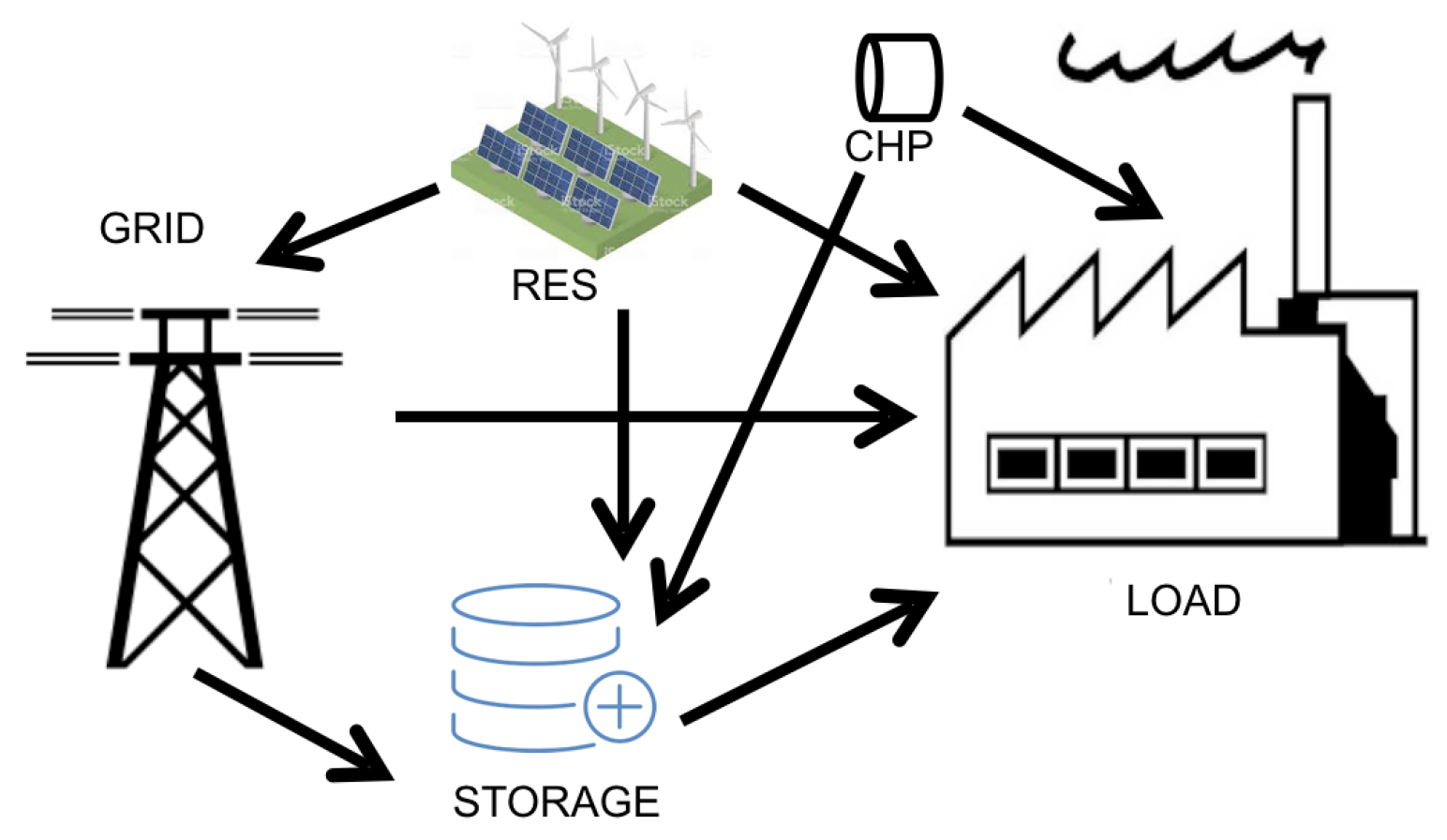
The Energy Management System (EMS) of a VPP (such as the one shown in
Figure 1) makes decisions by considering the energy prices and the availability of DER. In particular, it can decide:
the amount of energy that should be produced;
the generators that should be used;
if the surplus energy should be sold to the energy market or stored;
the demand side operations.
Optimization techniques applied to energy systems can improve their efficiency and stability (see, e.g., [
9]). The core of a VPP is an EMS that optimizes the power flows coming from the generators, controllable loads, and storages. In [
10] is presented an EMS for controlling a VPP. The objective of the model is to manage the power flows by minimizing the electricity generation costs.
Operating costs of complex energy systems can be reduced by techniques such as Demand Response (DR). DR improves energy efficiency by moving the energy consumption to lower price hours [
11] by being responsive to power market signals. Many optimization models [
12,
13] have been designed and implemented to support political and economical decision-makers (local governments and business developers) in choosing profitable and sustainable business models, regulation and tariffs.
Optimization techniques are generally used in the energy sector for planning and operational decisions. Recently, due to the increased uncertainty in these contexts, there is a growing need for enhancing the granularity and the horizon of the decisions. In the energy sector, all the most common techniques of optimization under uncertainty (e.g., robust optimization and stochastic programming) have been widely investigated [
14,
15,
16]. A frequent assumption to deal with uncertainty is that the future distribution of random variables is available through historical dataset or predictive models, or both [
17].
The critical decision process, consisting of deciding which generators should be active to minimize the system cost, can be defined as Unit commitment (UC). The deterministic UC formulation may not adequately tackle the impact of uncertainty. Therefore, ways to manage unit commitment under are the following uncertainty [
16]: (1) Stochastic UC, which is based on the definition of probabilistic scenarios [
15], and it usually requires high computational cost; (2) Robust UC, which is based on the definition of precise range for the uncertainty, instead of taking into account their probability distribution [
18]; (3) Hybrid models blend robust and stochastic approaches in order to balance positive and negative aspects of both methods [
19]. Forecasting techniques based on machine learning approaches have been applied for the prediction of flexibility of a VPP, taking into account its uncertainty. Some papers focused on the residential sector, by applying methods such as neural networks and support vector regression [
20,
21] with some promising results; but, they have not be implemented in the industrial sector by considering scalability.
In real-world applications, the optimization is also complicated by the fact that the optimization algorithm of the VPP has to make both medium/long-term decisions and short-term decisions: in the decision-making process models of the energy sector [
22], strategic goals must coexist with tactical, operational ones. These methods are meant to be the algorithmic cores of innovative architectures for energy systems that allow considering high degrees of resilience with respect to, for example, renewable energy sources, deviations from the estimated consumption plans, and with the ability to evaluate the system performance according to different metrics (costs, flexibility, stability of the system, or environmental aspects).
2.2. Market Simulation Techniques
VPPs participate in balancing markets by providing flexibility with respect to the declared demand profile. Each power system has its own balancing markets (BM). For example, in Italy, it is named dispatching services market (Mercato dei Servizi di Dispacciamento—MSD), and it is divided into several zones and sessions. For clarity, we will refer to it from now on with the term balancing market.
Participants of the market are agents of heterogeneous nature, dimension, and objective. Hence the power market is an extremely complex and interconnected system. Moreover, BMs rely on the results of the day-ahead markets and intraday markets. The balancing market is the way in which the Transmission System Operator (TSO) can assure the balance between generated and requested energy. So the BM have an intrinsically stochastic nature.
There are several ways to model the electricity markets [
23]. Works on modeling balancing markets price and/or quantities are rare since they depend heavily on the day-ahead and intraday markets and are therefore difficult to predict.
In general, market models (and hence, also BMs) can be divided into the following categories:
Multi-Agent models that rely on the modeling of each actor involved in the price formation. They are very flexible but rely on a high number of hypotheses. They are more fit for market design and policy analysis;
Structural models that rely on equations describing the relationship between the main influencing variables. (e.g., fuel prices, demand, temperature ecc.) Potentially very accurate, but require hard-to-acquire data and may have a big granularity;
Stochastic Process models, which try to model the price and quantity randomness via a stochastic process, with particular regard to spike prices. While not useful for punctual forecasting, they are rather used to model distribution on the medium-term, an aspect important for risk management and derivative pricing;
Statistical or Computational Intelligence methods that are similar to those used in other fields of energy analytics, such as load forecasting and generation forecasting.
The first three types are more suited for policy investigations, market design, risk management, and derivative pricing [
23]. The last group of methods is better suited for operational planning. These types of method are well established also in other areas of energy forecasting (see [
24] for a review of probabilistic load forecasting and [
25] for a general energy forecasting review).
According to [
26], BMs can be in one out of four states, in any given timestep:
Balancing market forecasting models are mainly divided into those that model the market state directly or indirectly (by looking at the sign of the forecast).
While market states are very difficult to predict punctually, the forecasting is still useful if it provides good probabilistic information. In any case, trivial forecasts can be hard to be surpassed in performance [
27]. In this paper, we used a simple probabilistic model based on historical data for simulating plausible outcomes of the market (see
Section 6.1.3).
2.3. VPP Projects
In recent years, several projects have tackled the issues related to VPP implementation.
For example, SmarterEMC2 project aimed at investigating whether the telecommunication infrastructure of today is able to support mass scale smart grid services such as demand response and DER integration in Europe, and also at supporting standardization endeavors. It involved both real-world VPPs and simulated VPPs [
28].
AGL Virtual Power Plant, is a prototypical VPP in southern Australia, connecting thousands of BESS and PV systems all coordinated via a cloud platform in both residential and commercial premises. It started in 2017 and is still ongoing [
29].
The eTelligence project, a four year project lasting from 2008 to 2012, involved a real test site in Cuxhaven, Germany. The site involved Wind, PV and Biomass generation, storage facilities, controllable loads such as a refrigerated warehouse, and other participants such as sewage treatment plants, swimming pools and private households [
30].
The FENIX project aimed at building a large scale VPP, taking in order to make DER participate in the power market and providing services to DSOs and TSOs. Validation was made with two field deployments, involving domestic CHP aggregation, wind farms, and industrial cogeneration [
31].
The EDISON project aimed at building a VPP composed of a fleet of EV cars in the Danish Island of Bornholm, investigating whether EVs can be useful in the context of VPPs [
32].
Finally, VPP4Islands project proposes technologies such as digital twin, virtual energy storage systems and distributed ledgers for multi-energy VPPs in the context of islands [
33].
2.4. Contributions
The VIRTUS project aims to implement a VPP in industrial contexts by focusing on both economic and energetic optimization, in order to provide services to the energy market. In particular, we consider and simulate all the principal actors of the system. The objective is to prove the feasibility of the synergic coordination of DERs for the local energy optimization from a technical and economic perspective.
In more detail, building upon such valuable and diverse projects in the state of the art, the VIRTUS project main contribution is to investigate scalability and communication bottlenecks in a modern VPP. In this sense, an important aspect of the project will be how the VPP affects distribution systems, and will provide guidance for their role in the future of Italian balancing markets. This will be validated using several pilot sites (a university, a hospital, an industrial plant) encompassing controllable and non controllable loads, BESS, PVs, commercial and industrial CHP, as well as a virtual test site, that will serve as a testbed for other VPP configurations and also for simulating other possible sources of distributed flexibility. Finally, the platform is meant to be tested on real industrial sites on a large scale, which will enhance the impact of the project.
3. A VPP Distributed Architecture
Based on the overview provided in the previous section, we can define the main objectives of a Virtual Power Plant: a VPP should optimally manage the single units, as well as providing support for the provision of balancing, regulation, and modulation services by responding to price signals.
Therefore, the final purpose of a VPP can be twofold: on the one hand offering flexibility towards the aggregator and on the other balancing locally consumption and production for a reduction of costs and an increase in flexibility. The VIRTUS project aims to analyze both aspects by aggregating responses to different requests of flexibility from the market based on energy prices and different configurations of local VPPs.
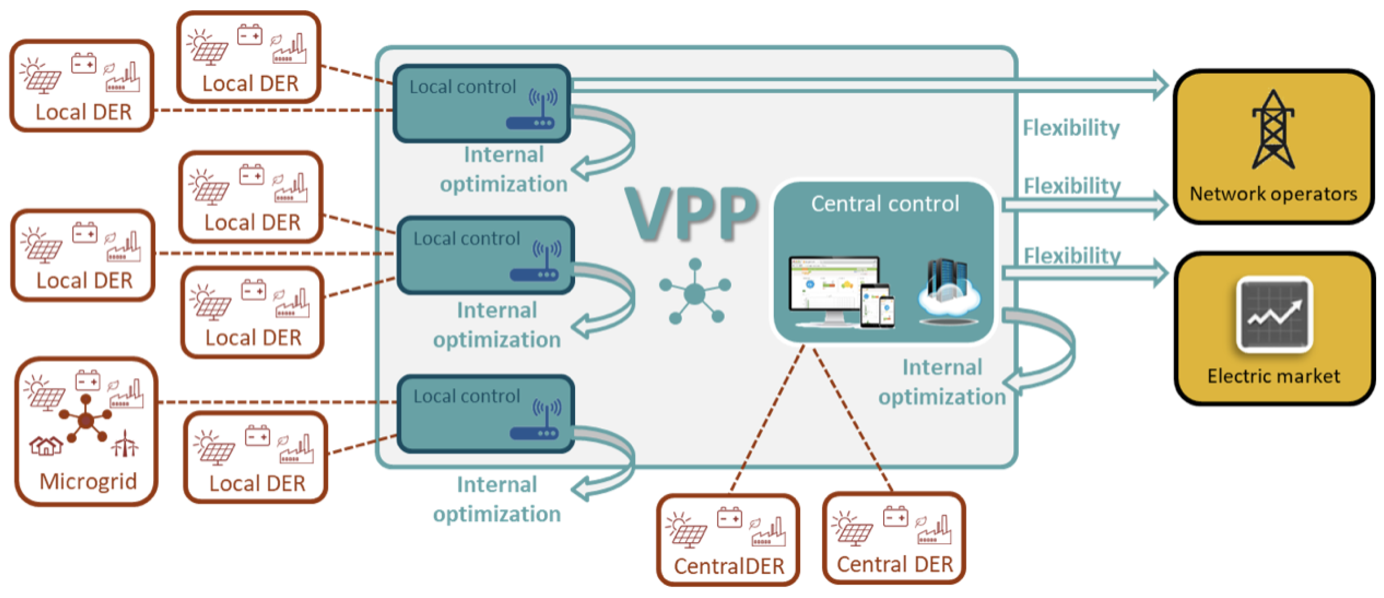
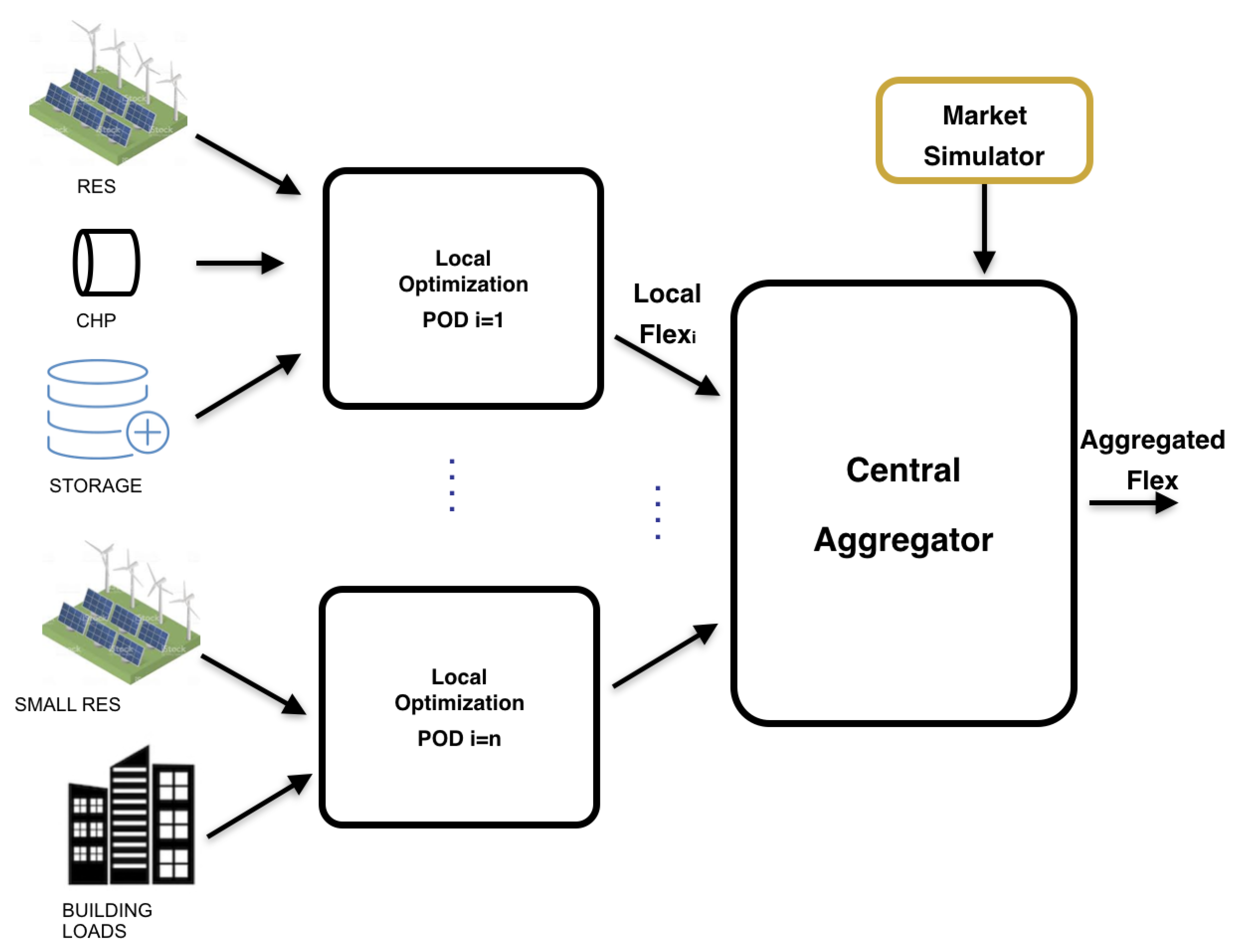
As shown in
Figure 2, the VPP is composed of a central aggregator and several decentralized control units and DERs. The latter can be of two types: the energy resources directly controllable by the central aggregator (indicated as Central DER) and those not directly controllable by it (indicated as local DER and/or Microgrid) but managed by decentralized control units. All these DERs (which can be viewed as local VPPs on their own) have to be optimized in order to offer flexibility towards the aggregator and then to the market. Based on these different configurations, and by considering a two-step robust optimization model, it is possible to evaluate the degrees of flexibility offered by the whole VPP. Please note that we consider this two-step architecture because, in an industrial context, it is common for the VPP clients to have their own EMS.
The flexibility of the VPP consists in the ability to quickly modulate and compensate for the variations in power required, and this is the result of the flexibility of the single local DER. It is a precious feature for the energy system: through rapidity in adapting to the quantity of electricity required, it is possible to better follow the price of energy on the market, thus offering the electricity produced aggregated effectively on the market.
Indeed, the value of electricity varies continuously and is subject to changes with often significant price differences. Load reduction programs could be significantly cheaper than building new power plants to meet peak load demand, and therefore analysis of demand response has taken importance with the consequent development of planning algorithms and business models (i.e., DSM). Furthermore, it is possible to estimate the flexibility offered by making strategic decisions to improve the real-time optimization of the aggregated energy schedule [
34].
4. Libra Platform
Within the VIRTUS project, a cloud platform (named Libra) for the management of VPPs in industrial and tertiary contexts is being developed. Aim of the project is to demonstrate the feasibility of the coordination of DER and local energy optimization for the provision of services to the various players in the electricity system, from a technical and economic perspective.
To this end, a group of pilot VPPs is proposed in the project:
a university VPP (20 buildings of the University of Genova);
a hospital VPP (14 buildings and two cogeneration plants of San Martino Hospital, located in Genoa, Italy);
an experimental industrial microgrid named Pontlab (located near Pisa, Italy) [
35].
Moreover, a simulated VPP is considered in order to test, for instance: the scalability of the solution, possible future scenarios, extreme exogenous conditions, and impact of the aggregation on the distribution network. This allows great flexibility and usability in inserting new types of components. The available modeled components of the simulated VPP are:
Generator: photovoltaic, wind energy, Combined Heat and Power (CHP);
Load: On/Off, HVAC, industrial process;
Energy Storage Systems: Batteries.
It is also possible to include entire smart local VPPs, without modeling their components (see PONTLAB [
35]) or mixed configurations of available components in the VPP).
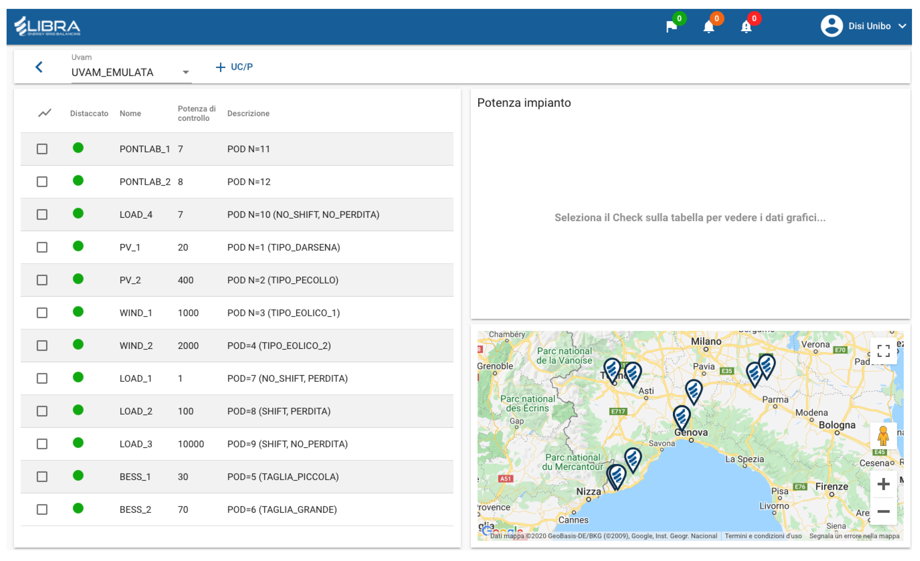
In
Figure 3 the VIRTUS simulated aggregation with its components is represented.
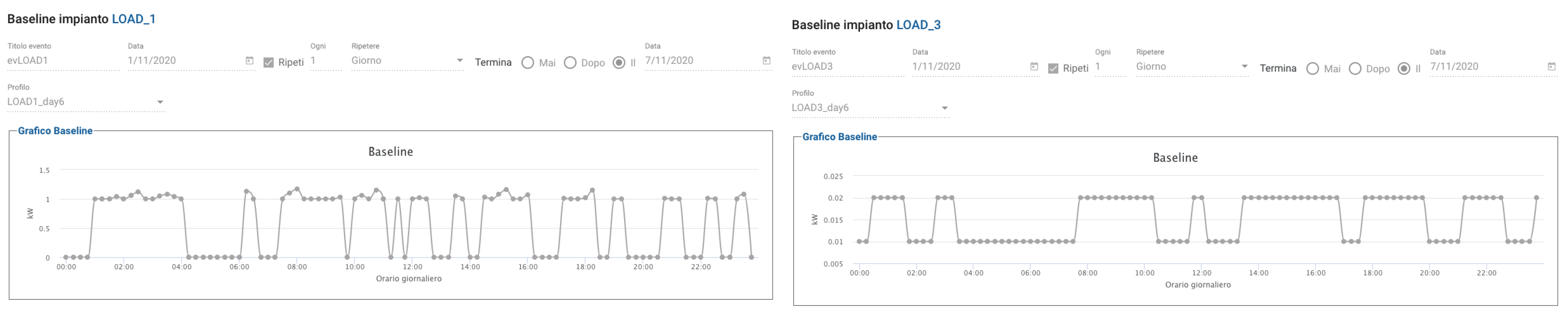
For each component, it is possible to provide real-time active and reactive power measurement (in kW and kVAr respectively), a daily range of upward and downward flexibility together with its cost (in kW and EUR/kW), optional state parameters of the component (e.g., the state of charge for a storage system), and a daily baseline (in kW), which is defined as the predicted 15-min net power profile of the units that constitutes the VPP. These baselines have to be communicated to the TSO before the market closing, according to the Italian grid code [
36].
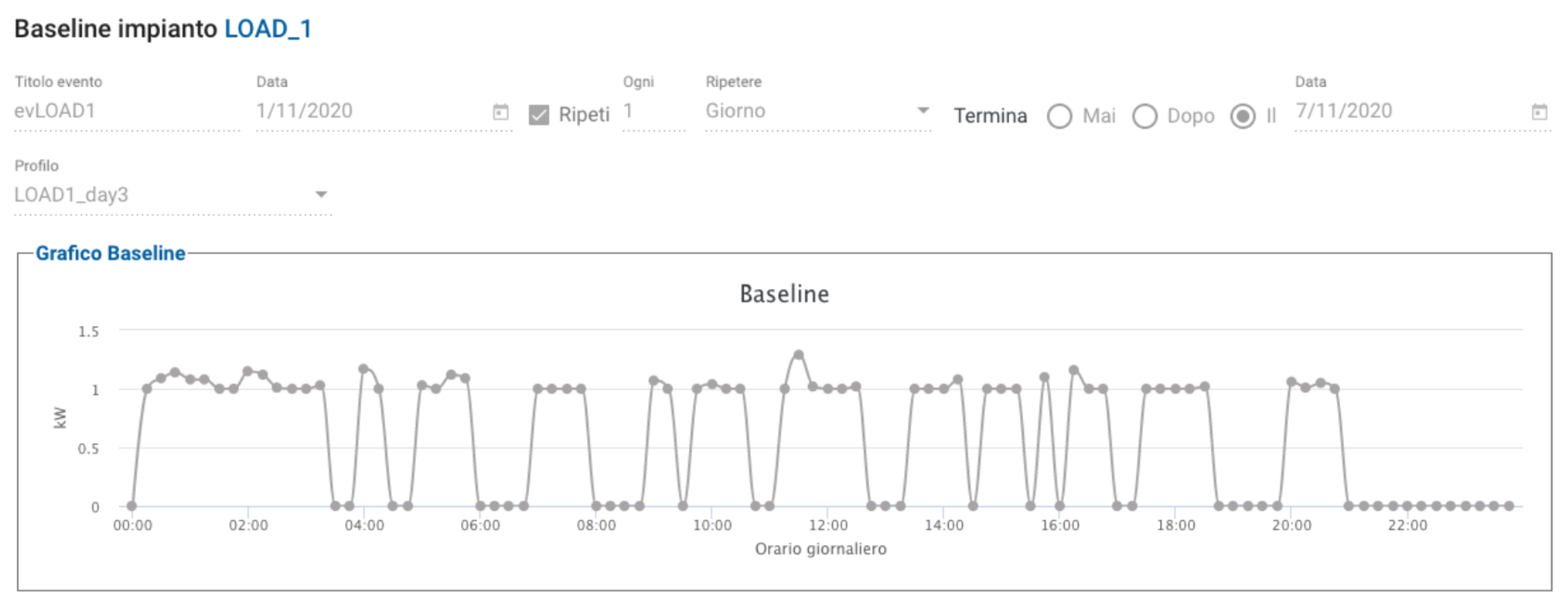
On the LIBRA platform, it is possible to graphically view the data of each plant by choosing a reference date and the information desired.
Figure 4 shows the baseline (96 timestamps) in kW for a selected date and for a selected plant in the VPP (e.g., LOAD_1).
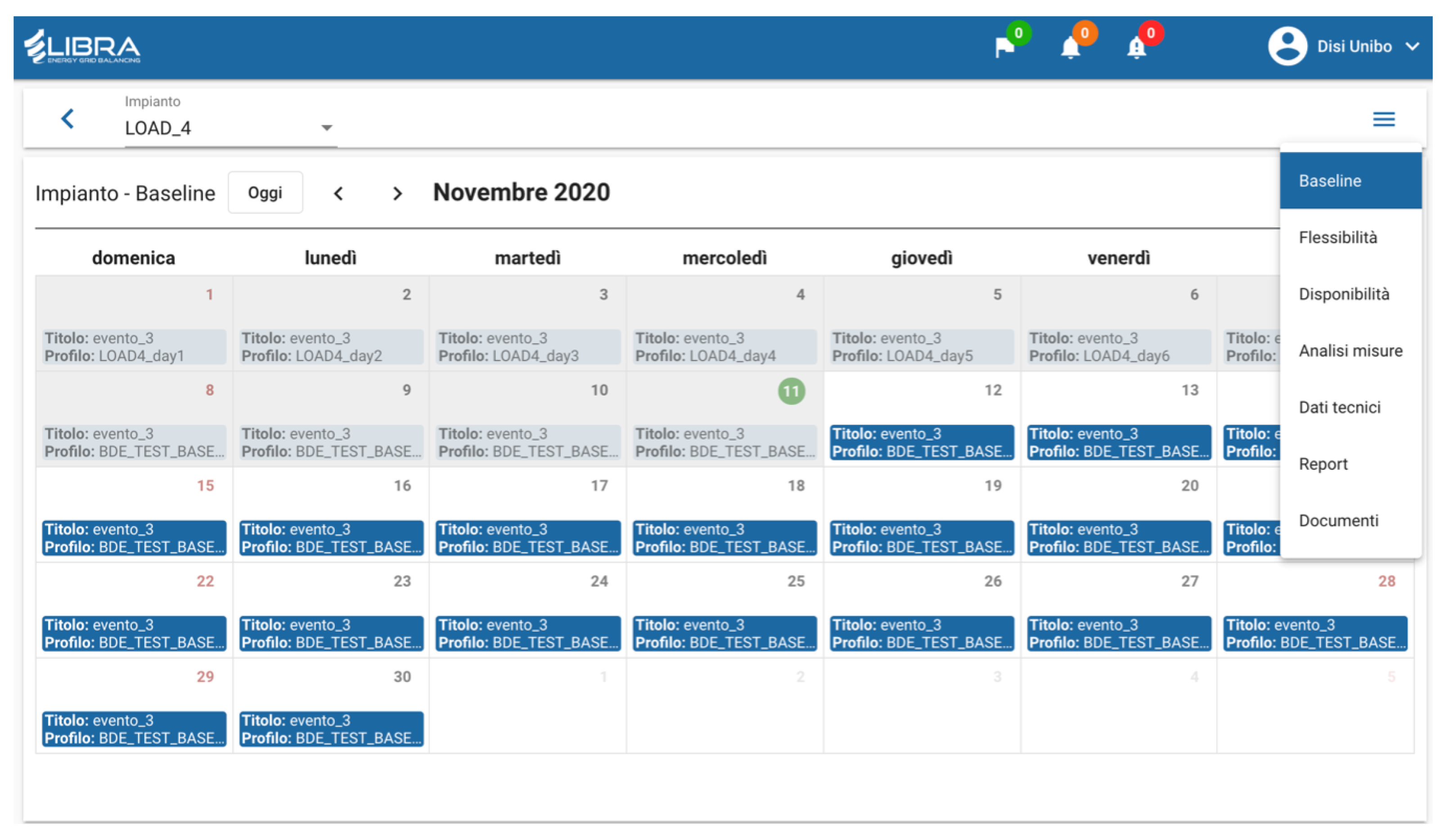
As with the baseline, the minimum and maximum flexibility of each component can be viewed and read via the User Interface (UI).
Figure 5 shows the load component called LOAD_4 and the menu for choosing the data to be displayed.
5. Optimization Model Description
The number of resources involved in the computation of the VPP flexibility can be really high and different in type and geographical distribution: this may pose a challenging computation effort and time constraints for the central optimization. We, therefore, introduce two different levels of optimizations: (1) a local optimization and (2) an aggregated optimization. In the first case, we optimize at the local level. A local VPP is a Point Of Delivery (POD) which owns and manage different type of DERs. To manage these DERs, a local optimization is run, and its result is communicated to the central aggregator of the VPP platform. In this case, the VPP does not need to know the internal composition of each POD: it can be seen as a small VPP into a large VPP. The VPP receives the declared flexibility resulting from the optimization of the local PODs, and it can manage it in order to provide an aggregated flexibility to the market.
5.1. Model Structure
The overall model structure is illustrated in
Figure 6.
Each POD can be considered to be a stand-alone VPP, with its internal DERs such as Photovoltaic, Wind and CHP production and industrial loads. Each local optimization is composed of two sub-optimizations: the first maximizing the use of his internal sources, the second minimizing it. Those values result in a range of POD flexibility that is sent to the VPP. The task of the central VPP is to collect all the flexibilities that come from the PODs and to optimize them in order to obtain at each timestamp the overall maximum flexibility. After that, the VPP is able to answer market requests of flexibility.
5.2. Local Level of Optimization: POD Optimization
A point of delivery can be considered to be an independent site composed of a set of mixed DERs. Each mixed POD makes an internal optimization of his resources, and then it communicates directly its range of flexibility to the central aggregator. For PODs composed of a single component (i.e., central DERs), we consider a direct connection with the central aggregator without local optimization.
In the next subsections, we present the local optimization model via Mixed Integer Linear Programming (MILP) formulation. The uncertainty of the system (i.e., renewable production and load forecasts) is tackled with Robust Optimization techniques that use a range for the uncertain instead of considering their probability distribution. We define the range of uncertainty as composed by the upper and lower bounds on the uncertain elements at each timestamp. Differently from stochastic techniques that minimize the total expected cost, robust methods reduce the costs of the worst cases for all the uncertain parameters.
5.2.1. Model of POD Components
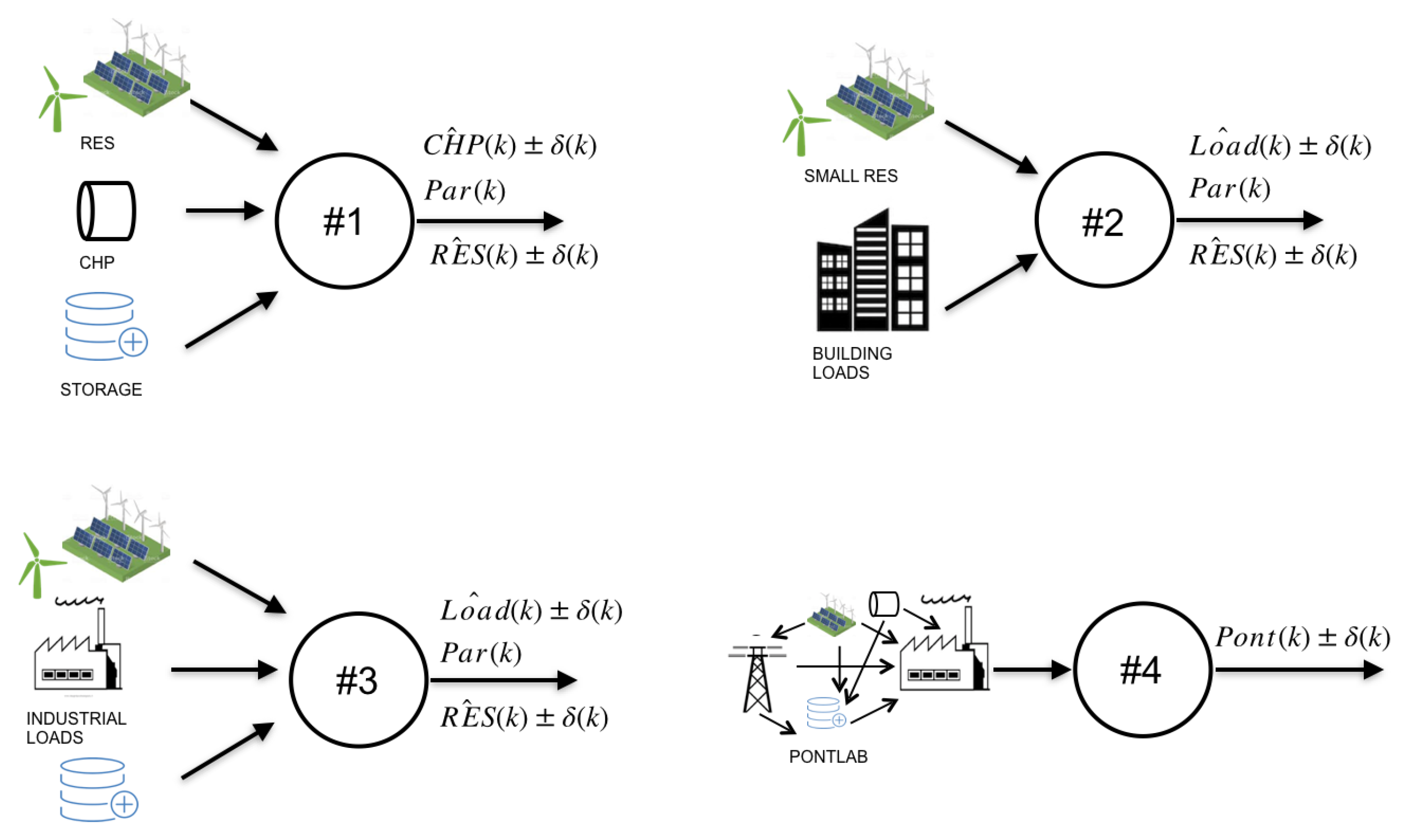
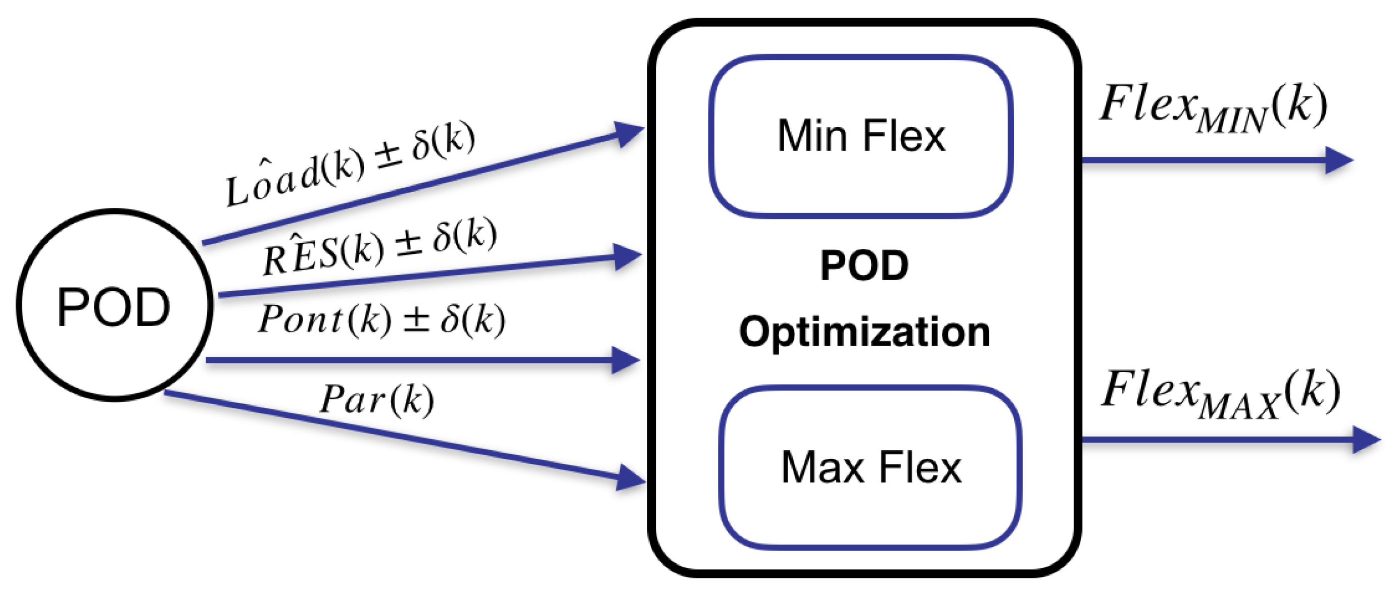
We propose an optimization model for the VPP EMS that is composed of two local optimizations: the first tries to fully cover the load by maximizing the use of internal DERs (minimum flexibility); the second tries to fully cover the load by minimizing the use of internal DERs (maximum flexibility). These two optimizations are computed for different configurations of local VPPs. We can see four POD examples with all components in
Figure 7, and a representation of the POD optimization module (with inputs and outputs) in
Figure 8.
To summarize, two different objective functions are considered:
This results in two bounds of flexibility made available for the central aggregator.
Formally, a local POD is modeled as an entity connected to a set G of “nodes” (e.g., generators, storage units …). Each variable represents the flow at stage k by considering the given baseline and the associated uncertainty for renewable production () or flexibility () for the other components. All technical parameters for each node are represented by .
In the optimization model, we assume the indexes refer to nodes representing the different types of loads (L1, L2, L3, L4), to storage units, to RES production (photovoltaic and wind), to the conventional generators (CHP), to the intelligent component endowed with an algorithm that gives the flexibility available to the aggregator, and to the external grid. All flows must respect the physical bounds and . The current state is encoded by the storage charge .
RES and Wind Production
We consider a robust approach based on prediction errors in the renewable power profile. Many researchers proposed methodologies for the estimation of global solar radiation on hourly intervals. Based on [
37], we consider as a prediction the average hourly global solar radiation. We focused on a defined period of data (summer period) reported in [
38,
39]. We make a further assumption: the prediction errors in each time period are modeled as random variables. We assume variables with a normal distribution and with the 95% confidence interval that corresponds to ±10% of the prediction value. In detail, the
δPV parameter for timestamp
k corresponds to 0.1
PPV(
k). Similar assumptions are made for the other renewable production sources considered (i.e., wind production).
For each time instant, we define an upper and a lower bound for the span of uncertainty. These bounds can be obtained by estimating confidence intervals. In Equation (
1) we consider 6 as index of RES, and we obtain the forecast of RES production composed by the baseline
for each instant
k, and a range of uncertainty
computed as explained above.
Storage Systems
Over the last decade, the development of storage systems (in particular, BESS) has increased, in order to cover the need for storing RES for the periods when they are not available. We model the BESS by defining the amount of energy stored at each instant k as a function of the power charged or discharged from the BESS unit in that timestamp.
We indicate the power exchange between the BESS and the VPP with
. The current state of the BESS is defined by a battery charge
, for each timestamp. The initial battery charge is
Equations (
2)–(4). We take into account of wear-off effects of the storage system by introducing a penalty cost for every time the corresponding flow changes direction (in the objective function that minimizes the total costs). The monetized impact
of such changes on the storage life cycle has been computed based on [
40]. The battery upper limit is
, and
is the charging/discharging efficiency: they are employed to specify the limits of the flow from/to the storage. We use the binary variable
, plus the indicator constraints in Equations (5) and (6) to track the direction of the flow. Whenever the flow changes direction, Equations (7) and (8) force the penalty flag
to be non-zero. The presence of the binary
variable makes the model a Mixed Integer Linear Program Equations (9) and (10).
Conventional Generators
We consider a CHP dispatchable generator, with associated allowed flexibility bound and cost for each timestamp. The optimization algorithm presented in this paper decides the quantity of generated CHP power for each timestamp. The quantity is composed by that are respectively the baseline and the delta of allowed flexibility that must be optimized by the local EMS.
Decisions concerning the CHP generation are considered
independent between each timestamp. We indeed hypothesize that each timestamp is long enough that the decision of switching on (respectively, off) the generator is independent with respect to the previous instants, by respecting the given parameters of allowed shift windows. Thus, The generated CHP power model is as follows:
where the bound are the given bounds of flexibility for the considered CHP generator. The local EMS can decide to shift the
to maximize or minimize the POD flexibility.
We underline that
(i.e., the baseline and the allowed flexibility for each timestamp, that is our decision variable) must respect:
Given some allowed time windows of shift (
), we have to maintain the total CHP production over all the time horizon, so we add daily conservation constraints to our model:
Intelligent POD as a Blackbox
The intelligent microgrid includes a small-size CHP, two thermal energy storages, a photovoltaic plant, a small wind turbine, and manageable thermal and electric loads. The optimization strategy [
35] is implemented to manage the operation of a CHP in RESs-heavy power systems.
The information needed for the central aggregator is only composed by a baseline (locally optimized as a blackbox) and a bound of flexibilities:
Demand Side Management for Loads
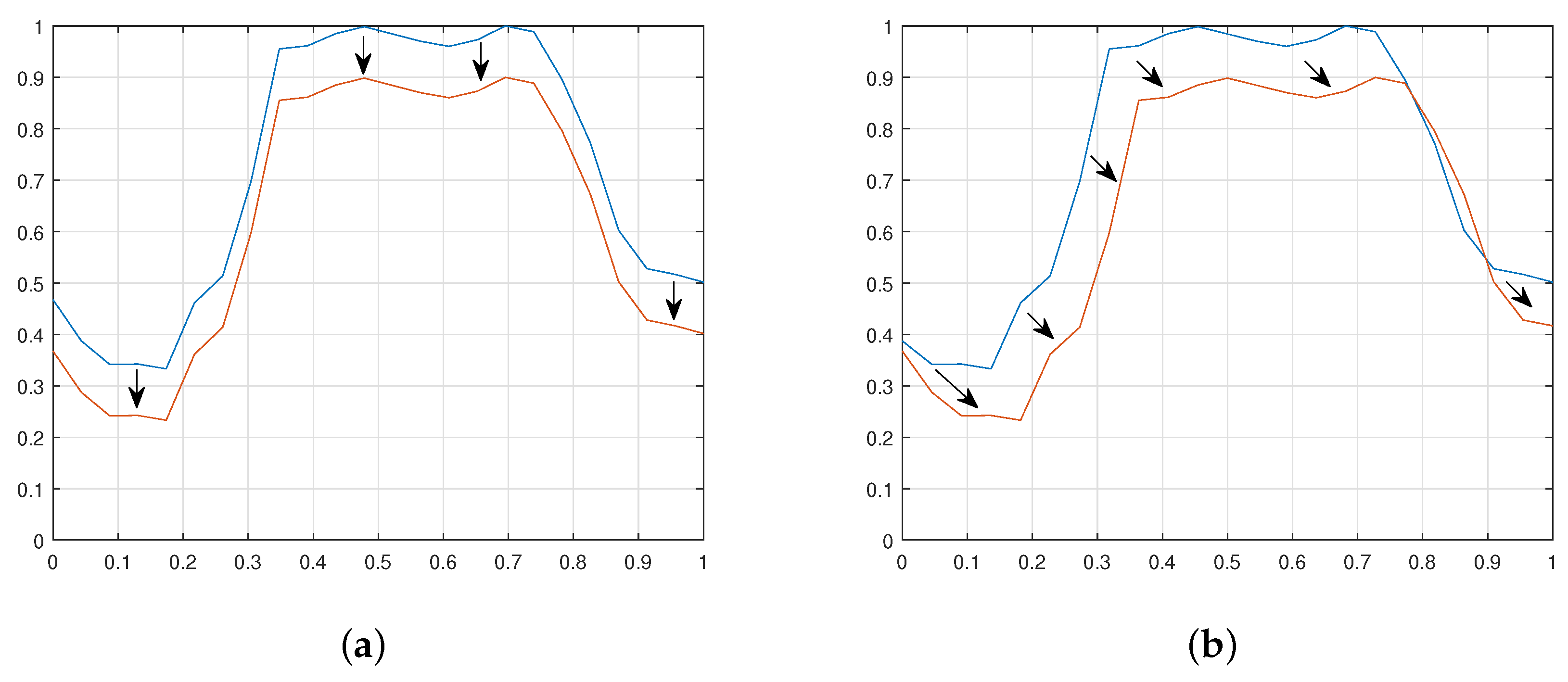
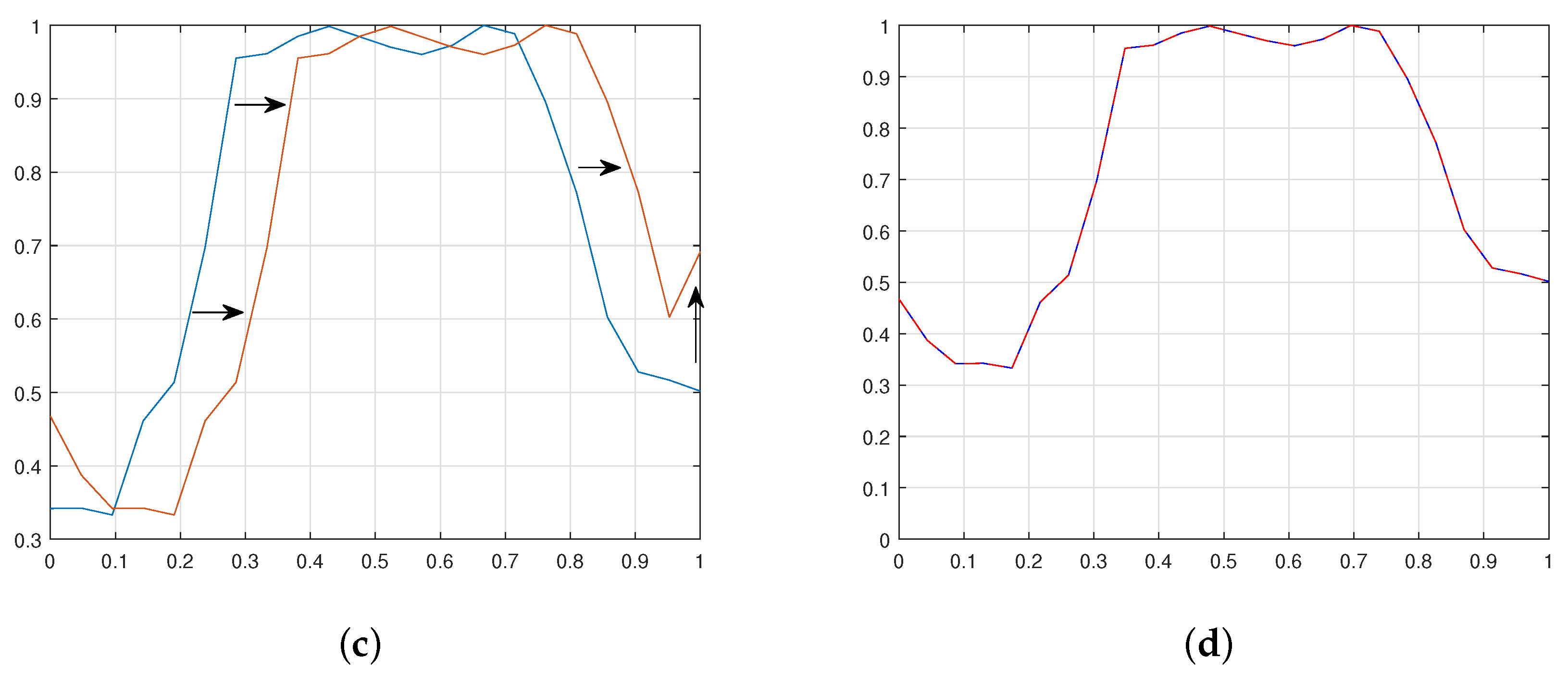
The DSM of our VPP model aims to modify the temporal consumption patterns for load components that allow it. Indeed, we consider four classes of load components:
L1 (sheddable load);
L2 (shiftable and sheddable load);
L3 (shiftable load with daily conservation);
L4 (non-controllable load).
In
Figure 9, the four types of modeled loads are exemplified.
L1 Equations (
16)–(18) is considered to be a sheddable load with a certain degree of allowed load reduction over the total time horizon. L2 Equations (
19)–(21) is considered to be a shiftable and sheddable load with some degree of shift (based on flexibility) and with a certain degree of allowed load reduction over the total time horizon. L3 (Equations (
22)–(24) is considered to be a shiftable load with some degree of shift (based on flexibility) but leaving the total amount of daily load constant. L4 (Equations (
25) and (26) is considered to be a total non-controllable load (i.e., with no degree of flexibility allowed over the given baseline).
We consider the same model for all the loads by changing the parameters. We recall that the already includes the robust uncertainty of the load forecasts. We assume that the total load on the whole optimization horizon is constant, and it could be with reduction or without reduction. More specifically, we assume that the consumption stays unchanged or with a reduction over sub-periods of the time horizon: for L4, this a possible way to state that demand shifts can make only local alterations of the demand load; for L3, we associate a reduction quantity. Formally, let be the set of timestamps for the n-th sub-period, the shifted load is given by:
Model for L4:
where
represents the amount of shifted load, and
is the originally load baseline for timestamp
k (part of the model input). The amount of shifted load is bounded by two quantities
and
. By properly adjusting the two bounds, we can ensure that the consumption can be reduced/increased in each time step by respecting the bounds. Deciding the value of the
variables is a goal of our optimization.
Power Balance
In general, ensuring power balance imposes that the total power generation must equal the load, , in all timestamps.
At each timestamp, the total load is covered by the generation of the internal DERs.
Overall, we have:
where
is composed by the sum of
Objective Functions
The first considered objective function of our EMS is the minimization of the expected flexibility
z (i.e., the exchange with the external grid) of the VPP over a time horizon (
T). The objective function formulated as:
The second considered objective function is the maximization of the expected flexibility (exchange with the external grid):
where the index 9 indicates the external grid. By minimizing the exchange with the external grid, we are forcing the local system to maximize the use of its internal DERs.
5.3. Global Level of Optimization: Aggregator Optimization
The number of internal resources can be really high (up to some thousand), and they can also be very spaced: this can leads to problems in terms of computation effort and time for a central optimization. That is why the concepts of point of delivery and central aggregator are introduced with two different levels of optimization: each POD makes a first flexibility optimization based on his internal resources and sends it to the central aggregator, which collects all the local optimized flexibilities from the PODs, and aggregates them to provide a range of aggregated flexibility to the market. This allows us to manage the scalability of our system: it is possible to make local POD optimizations in parallel, and the computational effort of the central aggregator can decrease considerably.
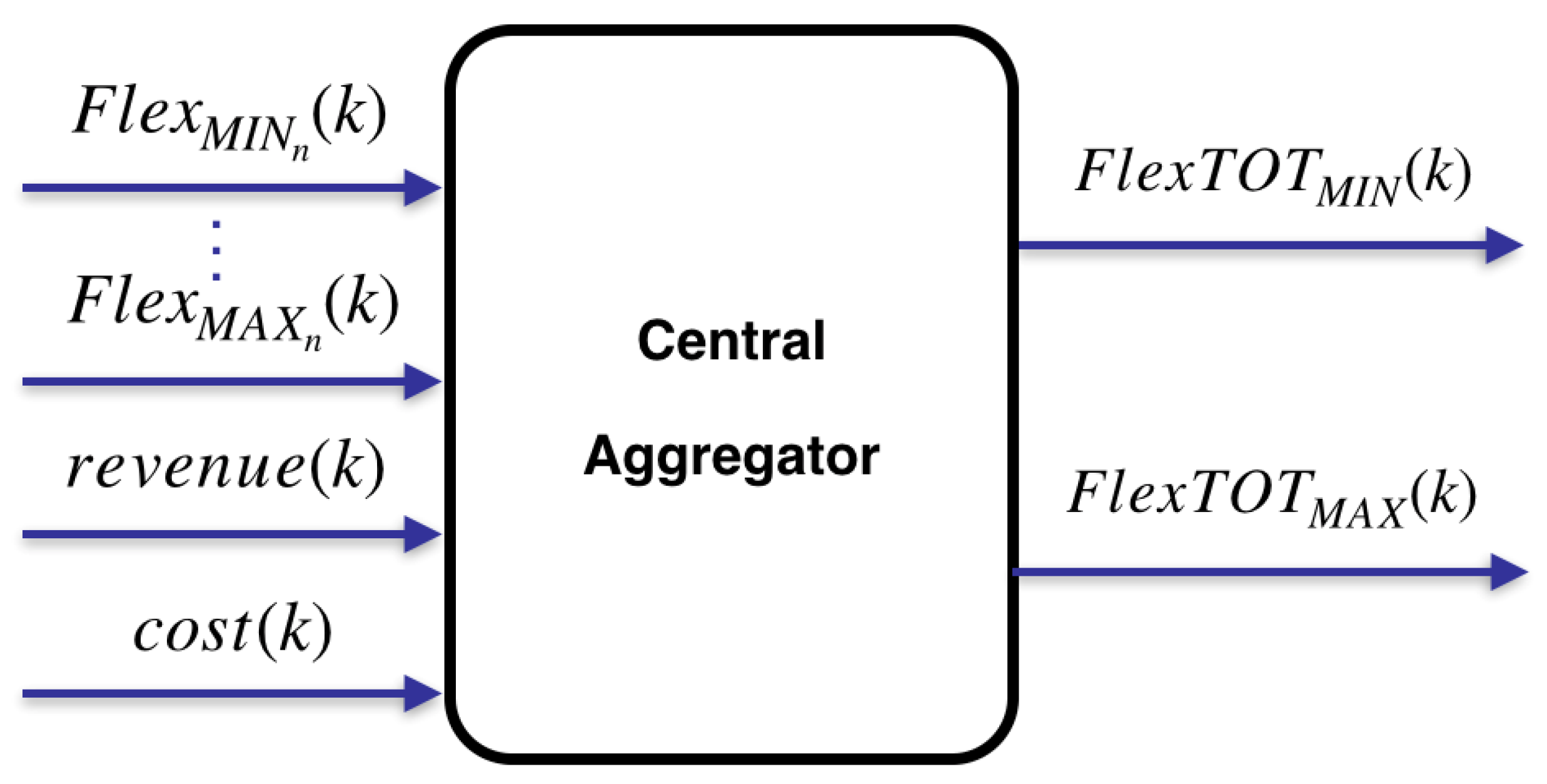
In
Figure 10 we can see the flexibility inputs of the central aggregator (i.e.,
and
) and the market revenues/costs given by the market simulator. The aggregator can also accept as input the flexibilities by single plants. In this case, the aggregator also has to consider the technical constraints of each plant in terms of flexibility (daily conservation or sheddable loads).
Given these inputs, the central aggregator maximizes the aggregated flexibility for all the involved local PODs
P at the maximum gain (i.e., minimum market cost) given by the market simulator.
The objective function Equation (32) is the maximization of the aggregated flexibility. We consider also market costs for each k (from the market simulator) in order to maximize the aggregated flexibility by minimizing the costs or maximizing the gains (we use = −).
In the next section, we will show the whole system implemented through a graphical simulation interface in order to test our optimization models over different configurations.
5.3.1. Local Optimization Recap
Model for storage systems:
Model for Renewable production:
Model for conventional generators:
Model for intelligent POD (Pontlab):
Objective function for maximization:
Objective function for minimization:
5.3.2. Aggregated Optimization Recap
6. VIRTUS Case Study
6.1. Detailed Architecture of the VPP
The optimization system of a VPP is based on a decision-making structure that allows high scalability and performance.
This section provides a detailed overview of each component, with the aim of clarifying their role within the VPP architecture of the project, highlighting the interaction between the components.
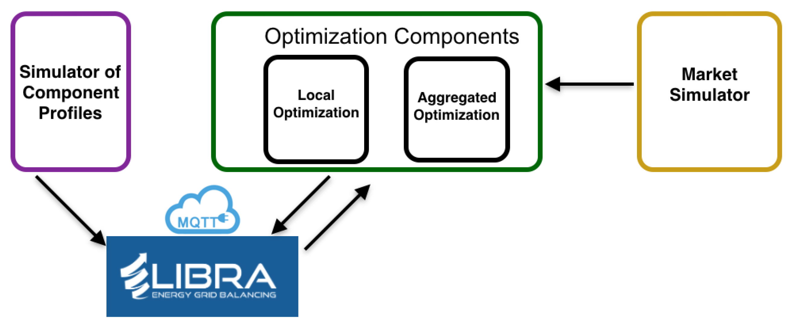
As shown in
Figure 11, three macro components of the VIRTUS architecture can be distinguished:
We can also notice that the VPP platform allows the communication between the different components of the system. For example, the simulator can pass state variables to the optimizers, while the optimizers can pass optimized setpoints to the LIBRA platform.
6.1.1. Profile Simulator
The VPP acts on several real, pilot sites. However, in order to test the scalability of the solution, a simulator is developed, which can be used to generate profiles related to components and PODs. These may model existent or non-existent sites for which we want to simulate future, extreme or hypothetical scenarios.
In practice, the simulator is a MATLAB software, which models generators, loads, and battery-based models. In the VIRTUS project, these components are planned to be located into a hypothetical grid and aggregated after running a power flow on the grid (see also
Section 8). The simulator also ensures that the variables that influence more than one component (e.g., weather) are treated uniformly among the components.
In
Table 1, the modeled components are summarized.
Generators modeled are:
PV (using the physical model presented in [
39]);
Wind (using the wind power model described in [
41]).
Loads modeled are:
Markovian Binary Loads. Given a nominal power P, a standard deviation s and a 2 × 2 transition matrix , a Markovian Binary Load is a load that can be in two states:
- -
Off (0 kW load);
- -
On ( kW load),
where is a normal random variable with 0 kW mean and standard deviation of s kW (with ). The transitions between the two states are governed by the M matrix.
HVAC (using historical data of the building described in [
42])
Industrial Load (using data retrieved from an open dataset [
43]
Each model is then considered to be L1, L2, L3, and L4 depending on specified options in the optimization model.
Battery Energy Storage Systems (BESS) are modeled using equations taking into account charging and discharging efficiencies (as in [
44]).
The intelligent pods are modeled by the algorithm presented in [
35].
The simulator sends the generated profiles to LIBRA, thanks to the MQTT broker. All the communication steps are illustrated in
Section 6.1.4 based on the User Interface of the system.
6.1.2. Application Scenarios
Within the VIRTUS project, five relevant aggregation scenarios have been defined based on the description of the services offered:
Cogeneration: N industrial microgrids that can be optimized locally, with hierarchical controller negotiating with the market. Services provided: DR mechanisms for peak shaving, load shedding, voltage support;
Contractualization of energy production from renewable sources (photovoltaic, wind, etc.). Services provided: frequency regulation, generation curtailment, downward reserve, voltage support;
Aggregation of N buildings with flexibility on Demand; Response. Services provided: DR, Peak Shaving, Load Shedding
Compensation of intermittent generation through activation of coupled storage systems;
Aggregation of different types of plants (by respecting grid constraints). Services provided: DR mechanisms for peak shaving, load shedding, frequency regulation, generation curtailment, downward reserve, Distributed Generation intermittent compensation.
In practice, based on previous scenarios, we define 5 application scenarios based on the components modeled in the profile simulator:
Application Scenario 1: Intelligent POD;
Application Scenario 2: PV and Wind RES;
Application Scenario 3: Load profiles
Application Scenario 4: PV and BESS;
Application Scenario 5: combinations of 2, 3 and 4
In our experimental analysis, we consider four different case studies based on Scenario 5 that considers mixed aggregation of plants in order to show the different degree of flexibility offered based on the aggregation considered.
6.1.3. Market Simulator
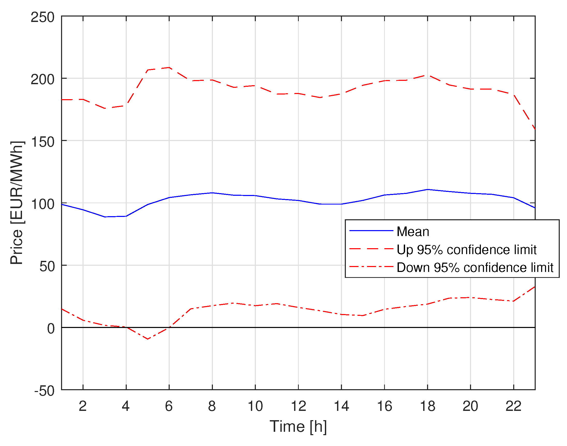
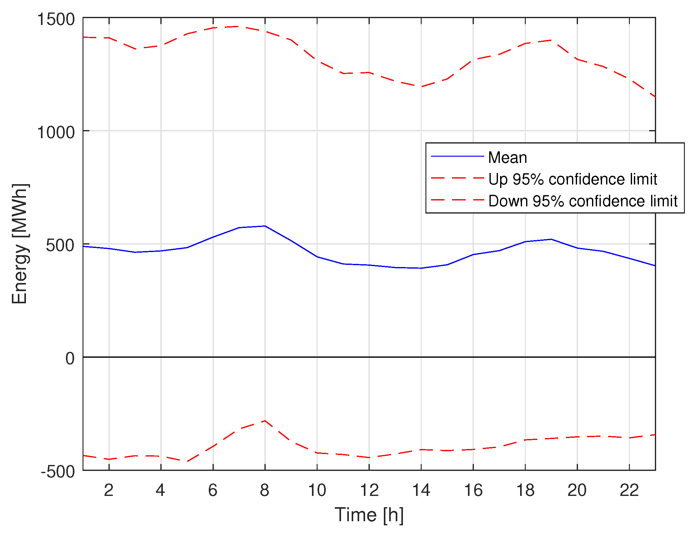
In this paper, prices and quantities are modeled using historical hourly data of the Italian balancing market from 2015 to early 2020, retrieved via the market regulator site, using the following procedure:
Missing data is omitted,
For prices, we discard maximum and minimum prices, and we focus on mean prices.
For quantity, we retain both upward and downward regulation
We retain the market zones of the real test-sites (North and Center-North of Italy)
We have therefore eight variables of interest:
- -
Mean Upward regulation price for North zone [EUR/MWh];
- -
Mean Upward regulation price for Center-North zone [EUR/MWh];
- -
Mean Downward regulation price for North zone [EUR/MWh];
- -
Mean Downward regulation price for Center-North zone [EUR/MWh];
- -
Upward regulation quantity for North zone [MWh];
- -
Upward regulation quantity for Center-North zone [MWh];
- -
Downward regulation quantity for North zone [MWh];
- -
Downward regulation quantity for Center-North zone [MWh],
for which we build a model capable of generating unseen yet plausible market data.
we assume the data to have a gaussian distribution, with parameters different for each variable and hour. In particular, mean and standard deviation is retrieved from the historical mean and standard deviation. Simulation is made by sampling from the estimated gaussian random variables. Let
s be the sampled quantity. Then the final simulated quantity is defined as:
Thus, no null quantity or price is simulated (note that the Italian market does not allow negative prices).
Figure 12 and
Figure 13 report the mean and the 95% confidence band for two representative model.
Please note that the confidence interval is quite large for both cases. This is a sign of high variability in the historical data for the considered period. This variability is partly due to the intrinsic stochasticity of the ancillary market, and partly due to important regulatory changes in the Italian Balancing Markets in recent years [
45].
6.1.4. Components Integration with the Netlogo Tool for Simulation
In order validate the entire system on a large number of plants and mixed scenarios, the different modules of the VPP have been integrated into a simulator developed in Netlogo [
46].
Netlogo is a tool for agent modeling and simulation and includes basic support for dynamic system modeling, offering a highly characterizable graphical interface.
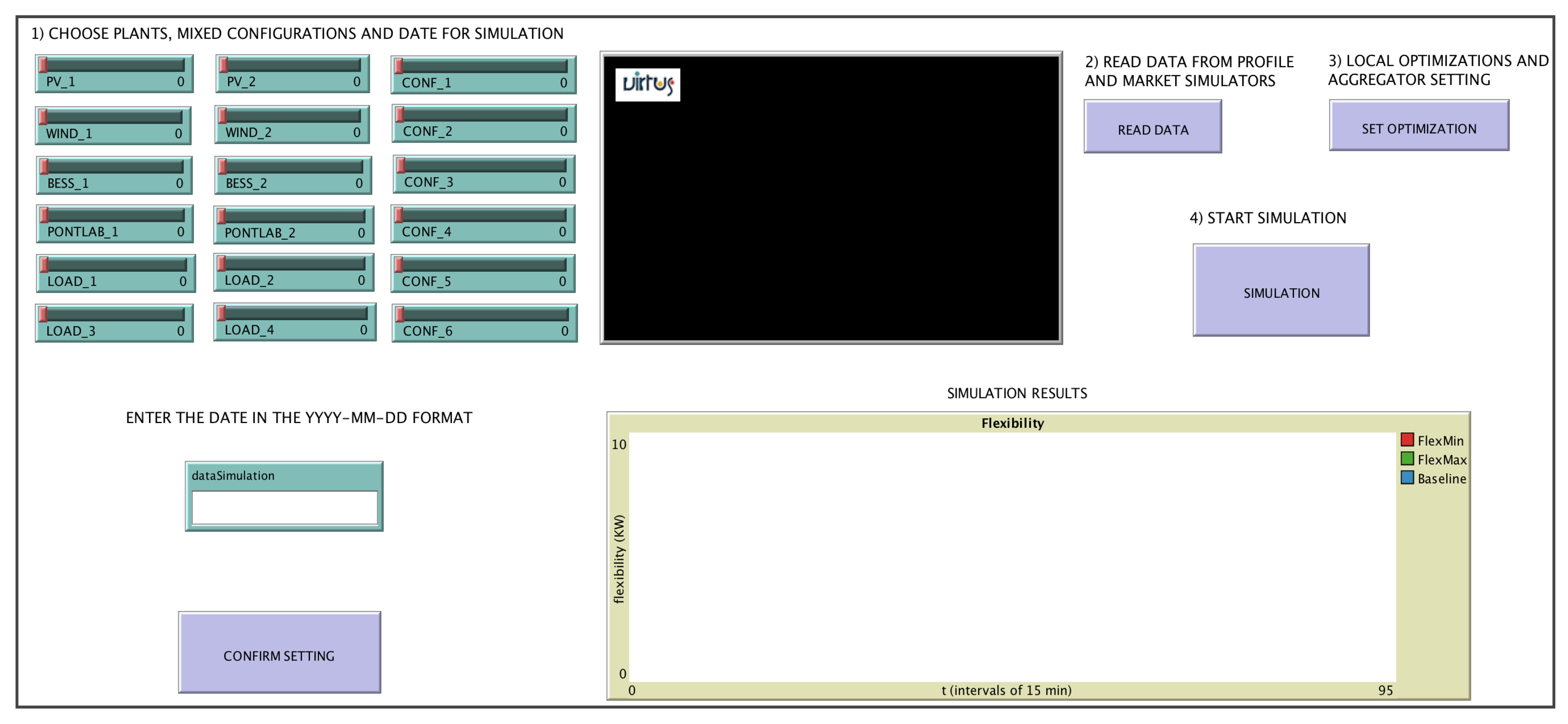
In
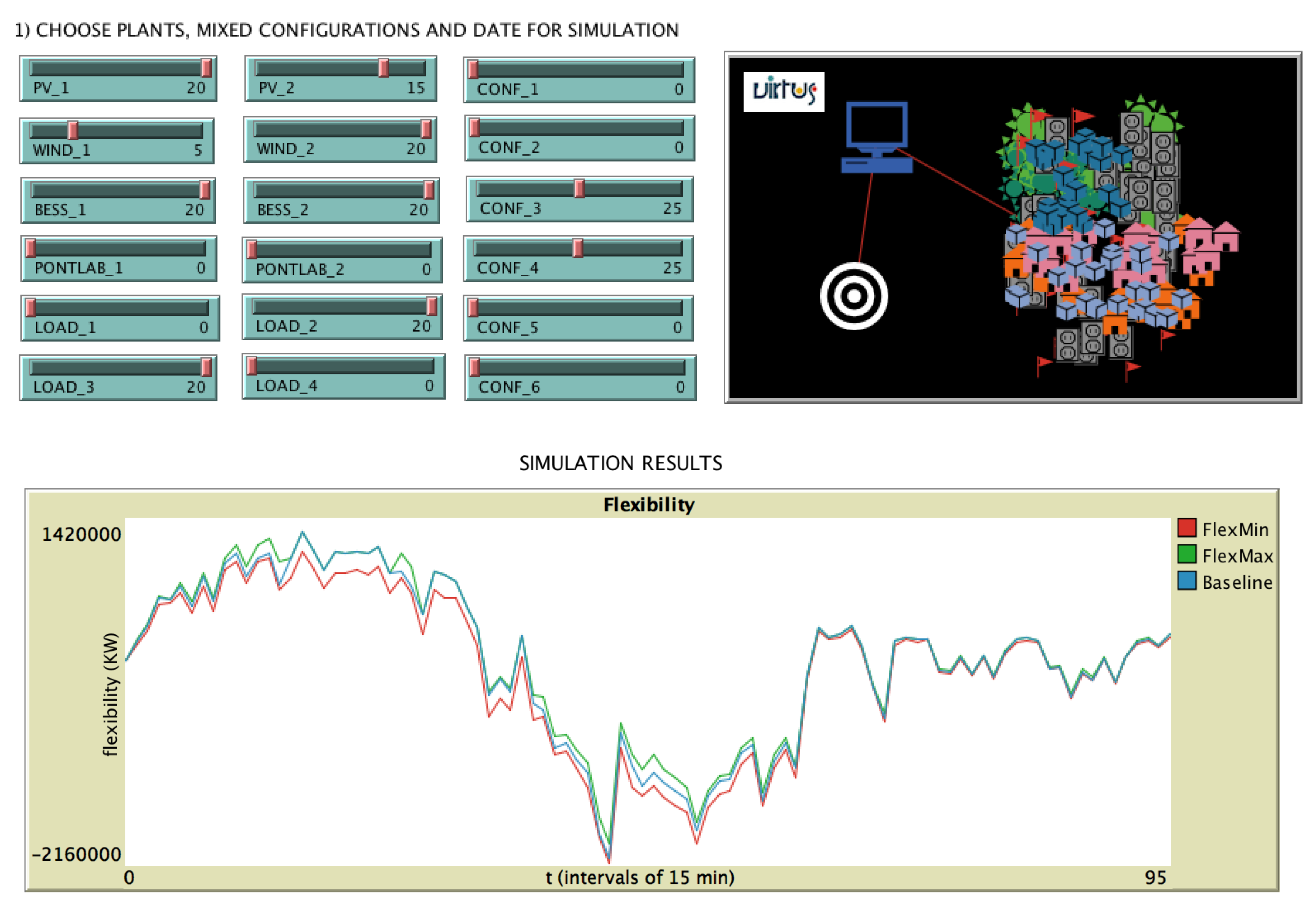
Figure 14 we show the interface of our system.
We can notice that we have the possibility to easily add and configure the number and the type of the plants that we want to involve in the simulation, by modifying the input data with the green sliders. By integrating our architecture in Netlogo, we create a single agent for every single plant (with configuration parameters) and an aggregated agent that is based on the optimization model of the VPP aggregator.
Through the graphical interface developed in Netlogo, it was possible to integrate the setting of the different input parameters and the configuration for each component, the communication via MQTT for data on the LIBRA platform, and, finally, the visualization of the aggregation and optimization results on plots. In particular, each plant is considered to be a single agent, each mixed configuration is considered to be an agent aggregation, and finally, the aggregator agent is at the highest level. It has the possibility of aggregating several agents of the lower levels using the optimization model of central aggregation.
An example of a graphic interface is shown in
Figure 14 in which it is possible to see how it is possible to set all the configuration parameters (number of each plant of the system and/or mixed configuration (POD), simulation date, etc.), activate the communication via MQTT with reading data from LIBRA, reading/writing csv between optimization modules, and finally viewing the results on the plot in the interface.
In general, the simulation consists of four steps:
Configuration settings (choice of the number of plants, PODs, and simulation date)
Reading data via MQTT from the platform (reading profiles, flexibility and technical parameters of each system of the setting required and present in the VPP on platform via MQTT, saving data for the local optimizer setting, if necessary).
Local optimization of mixed configurations, transfer of setting data to the central aggregator (passage via csv file of local optimizations of the flexibility and baseline of the system components chosen through the configuration setting)
Aggregated optimization through the aggregator agent, after reading the data from the market simulator in relation to energy prices for each instant.
We simulate six VPP configurations, which are based on application scenario 5
Section 6.1.2, previously introduced and summarized also in
Section 2 and
Table 2. In particular:
Conf1 is composed by: RES, BESS, L1, L4;
Conf2 is composed by: RES, L2, L3;
Conf3 is composed by: RES, BESS, L2;
Conf4 is composed by: RES, BESS, L2, L3;
Conf5 is composed by: RES, BESS, L1;
Conf6 is composed by: RES, L1, L4.
The optimization modules are implemented in Python using the Gurobi solver [
47].
7. Results and Scalability Discussion
In this section, we present the optimization module scalability experiments and their numerical results. The experiments have been carried out on four test cases. The case studies are composed of the plants specified in
Table 3.
7.1. Experimental Setting
We consider four complex case studies to validate our system:
Case study 1: RES production, no BESS, loads without shift, and combination of the previous resources;
Case study 2: RES production, BESS, loads without shift, and combination of the previous resources;
Case study 3: RES production, no BESS, loads with shift, and combination of the previous resources;
Case study 4: RES production, BESS, loads with shift, and combination of the previous resources.
The aim is to assess the numerical scalability of the VPP. Additionally, we will show in our results how flexibility changes based on the presence/absence of BESS and flexible loads. We carried out the four case studies with the same simulation setting (i.e., the same flexibility request, same date, and same market prices) to show the different responses of the aggregator. We underline that we use the passive sign convention (negative values for generation and positive values for load).
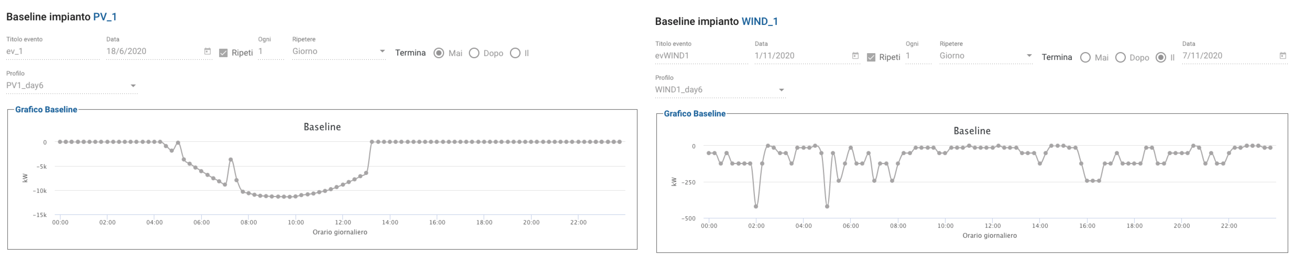
The experimental setting is based on a period of 7 days (1–7 November 2020) and in
Figure 15 and
Figure 16 an example of baselines for the day 6 November 2020 is shown for the considered plants of the VPP.
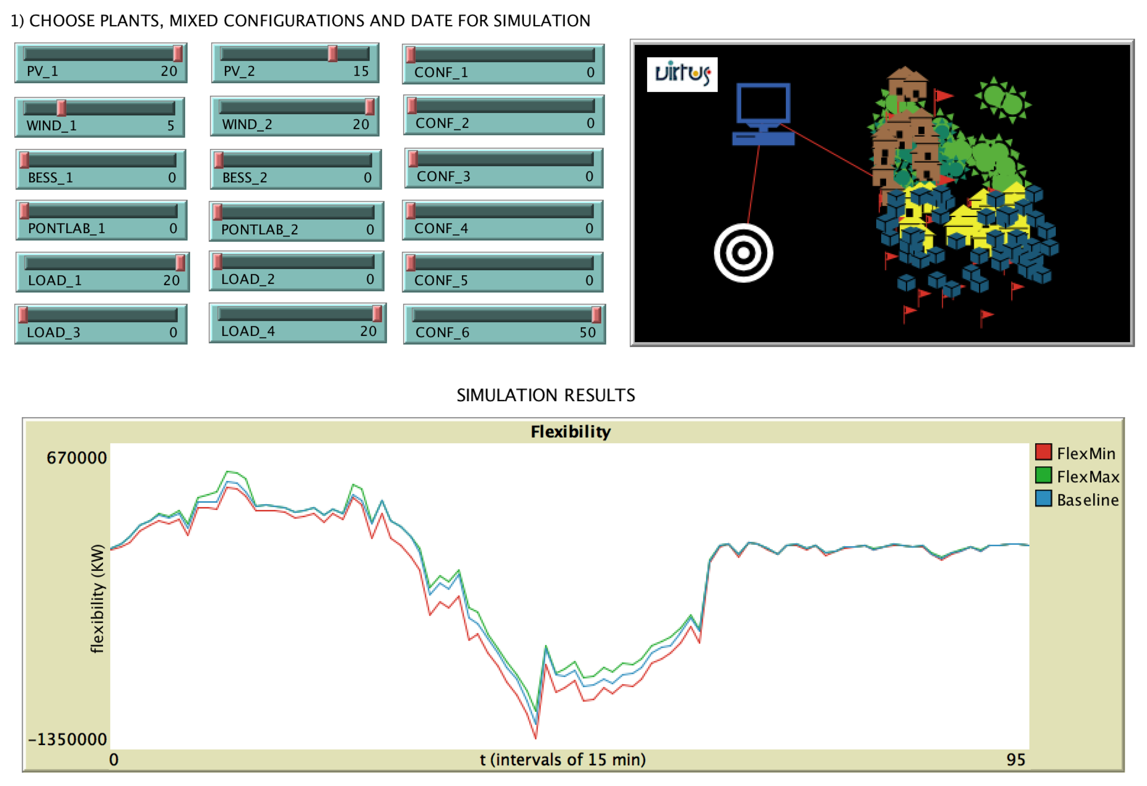
7.2. Case Study 1
The first case study is composed of RES production, no BESS, loads without shift, and a combination of the previous resources (see
Section 6.1.2 for further details). In detail, it is composed by (see
Figure 17):
20 plants of PV1, 15 of PV2, 5 of WIND1, 20 of WIND2;
no BESS;
Load without shift: 20 plants of L1 and 20 plants of L4;
Mixed configurations with no BESS and no shiftable loads: 50 plants of Conf6.
To run the simulation used for the case study comparison, we use:
the same market prices (i.e., Mean Up/Down regulation price for Center-North zone [EUR/MWh]);
the same date (i.e., 6 November 2020).
As shown in
Figure 17, the range of flexibility is greater in the central hours of the day (12 am–6 pm) when higher renewable production is expected, in particular with respect to the last parts of the day (after 6 pm). We can assume that this is due to the absence of BESS and shiftable loads so, in the following case studies, we add these components to simulate the different responses of the system.
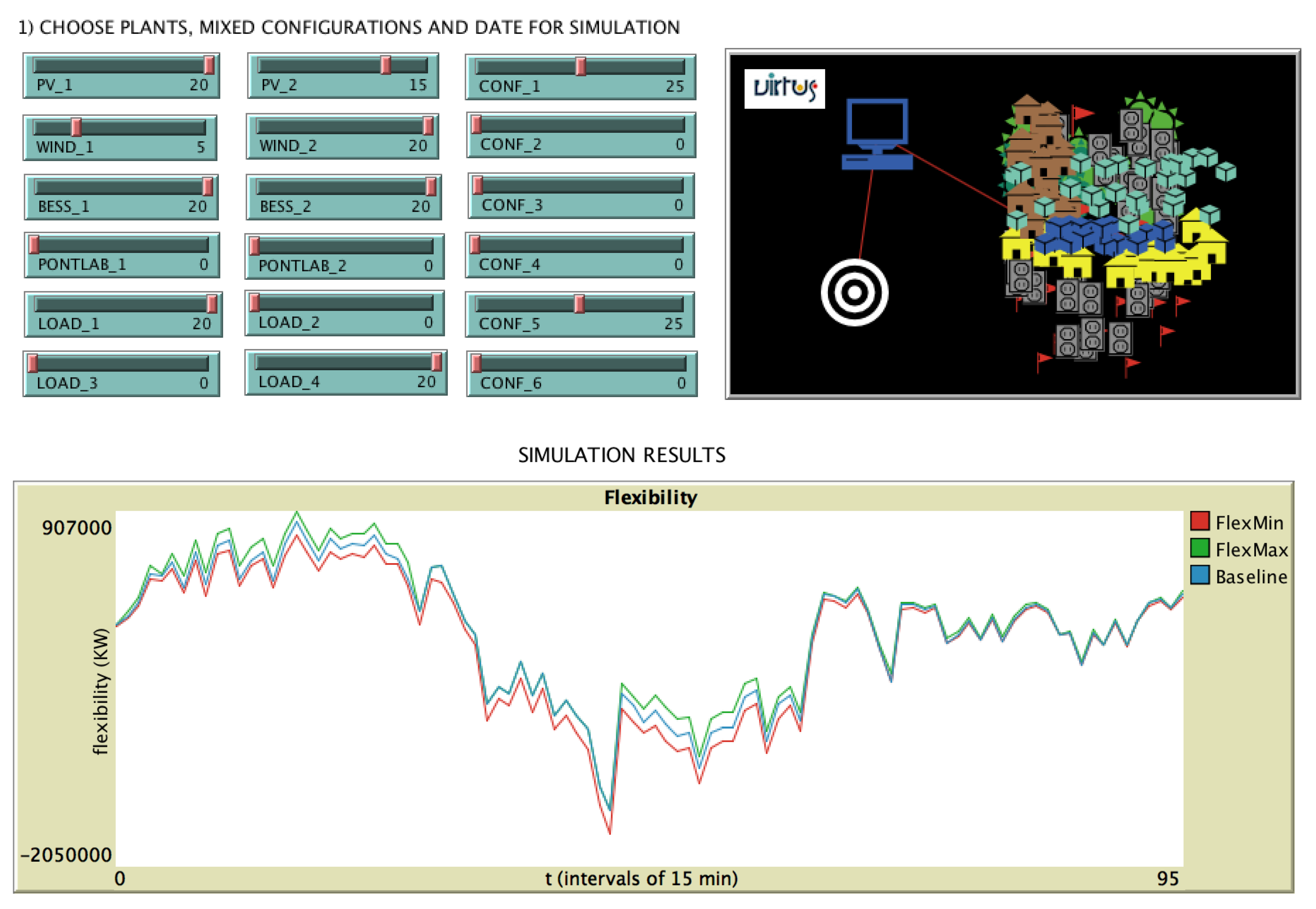
7.3. Case Study 2
In this case study, we add BESS plants to our system. Hence, the second case study is composed of RES production, BESS, loads without shift, and a combination of the previous resources (see
Section 6.1.2 for further details).
In detail, it is composed by (see
Figure 18):
20 plants of PV1, 15 of PV2, 5 of WIND1, 20 of WIND2;
20 plants of BESS1, 20 plants of BESS2;
Load without shift: 20 plants of L1 and 20 plants of L4;
Mixed configurations with BESS and no shiftable loads: 25 plants of Conf1, 25 plants of Conf5.
As shown in
Figure 18, the range of flexibility, differently from the previous case study, is quite wide during the whole time horizon, in particular in the first part of the day (before 10 am), through BESS systems. We can notice that in the last part of the day (after 6 pm), there is a minimum (almost absent) range of flexibility, probably due to the absence of shiftable loads. We try, in the following case study, to add shiftable loads to the system (instead of BESS) to simulate the different responses.
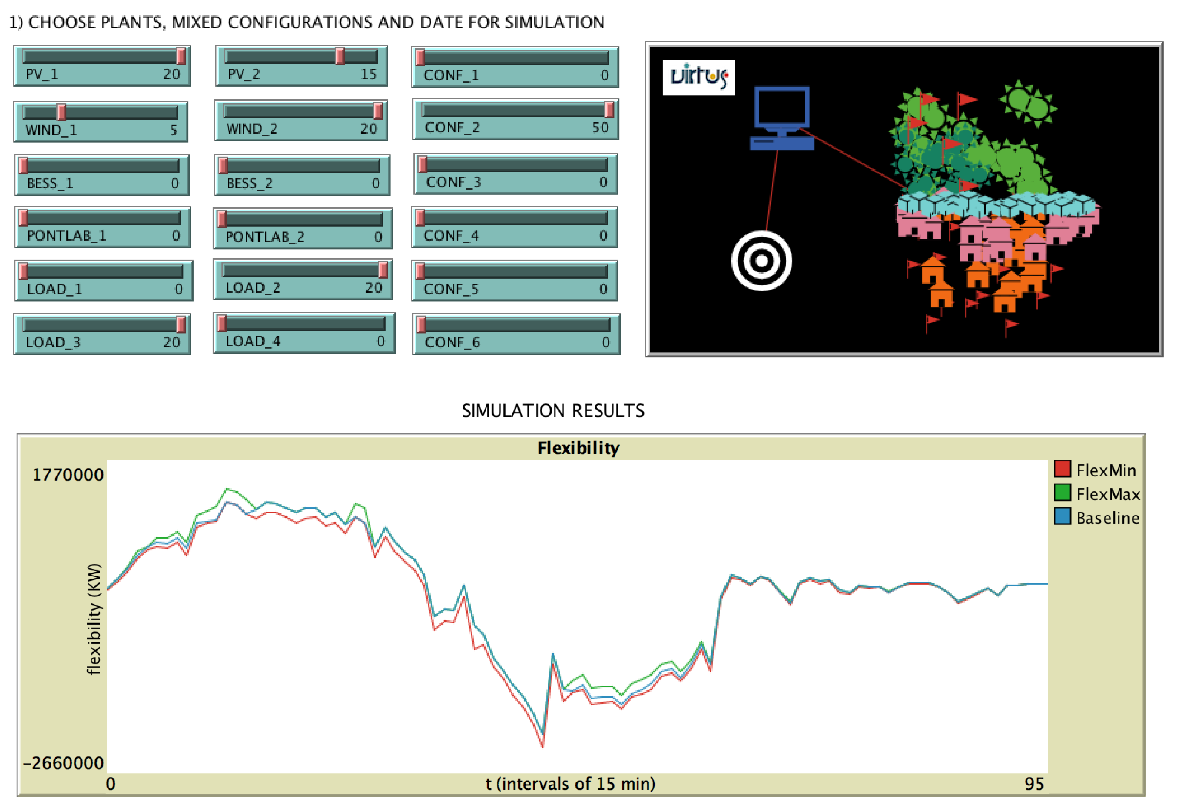
7.4. Case Study 3
To improve the flexibility during the first part of the day, we try to add shiftable loads to our system. Then, the third case study is composed of RES production, BESS, shiftable loads, and a combination of the previous resources.
In detail, it is composed by (see
Figure 19):
20 plants of PV1, 15 of PV2, 5 of WIND1, 20 of WIND2;
no BESS;
Load with shift: 20 plants of L2 and 20 plants of L3;
Mixed configurations with no BESS and shiftable loads: 50 plants of Conf2.
As shown in
Figure 19, the mere presence of shiftable loads without BESS is not sufficient to increase the range of flexibility. We can see a reduction in the range during the first part of the day (before 10 AM) and an almost absent range of flexibility during the last part of the day (after 6 pm). In our last case study, we try to add both shiftable loads and BESS.
7.5. Case Study 4
To improve the flexibility during the first and the last parts of the day, we try to add flexible loads and BESS to our system. Then, the fourth case study is composed by RES production, BESS, loads with shift, and combination of the previous resources.
In detail, it is composed of (see
Figure 20):
20 plants of PV1, 15 of PV2, 5 of WIND1, 20 of WIND2;
20 plants of BESS1, 20 plants of BESS2;
Load with shift: 20 plants of L2 and 20 plants of L3;
Mixed configurations with BESS and shiftable loads: 25 plants of Conf3, 25 plants of Conf4.
In
Figure 20 we can notice that the presence of BESS allows maintaining a wide range of flexibility during all the time horizon. Additionally, in this case study, in the last part of the day (after 6 pm), the VPP is not able to guarantee a broad range of flexibility. We can see only small variations in this case study, probably due to the presence of both shiftable loads and BESS. We can assume that the storage systems would be unable to guarantee flexibility for the entire time horizon. We will try to extend in future work the experimental setting by considering different types and sizes of storage systems.
7.6. Execution Time Comparison
To further show the integration of the different levels of optimization and to stress the possibility of improving the scalability of our system, we make a time comparison in
Table 4.
In
Table 4 we can notice that we are able to optimize ~170 plants/configurations in a total optimization time of ~10 s. We recall that this total time is composed of the sum of the local optimization time (i.e., the time for the optimization of all the mixed configurations) and the aggregation time (i.e., the flexibility optimization that aggregates all the mixed configurations and the single plants present in the system). We can see that increasing the number of single plants affects the total time of optimization less than increasing the number of mixed configurations, because the computation time is mostly due to the local optimization time, which is in turn due to the mixed configurations. This is clearly due to the need for a local optimization that can, however, be parallelized if we need better performance in view of a further increase in scalability. In
Table 4 we also show the
and
times over 30 simulations.
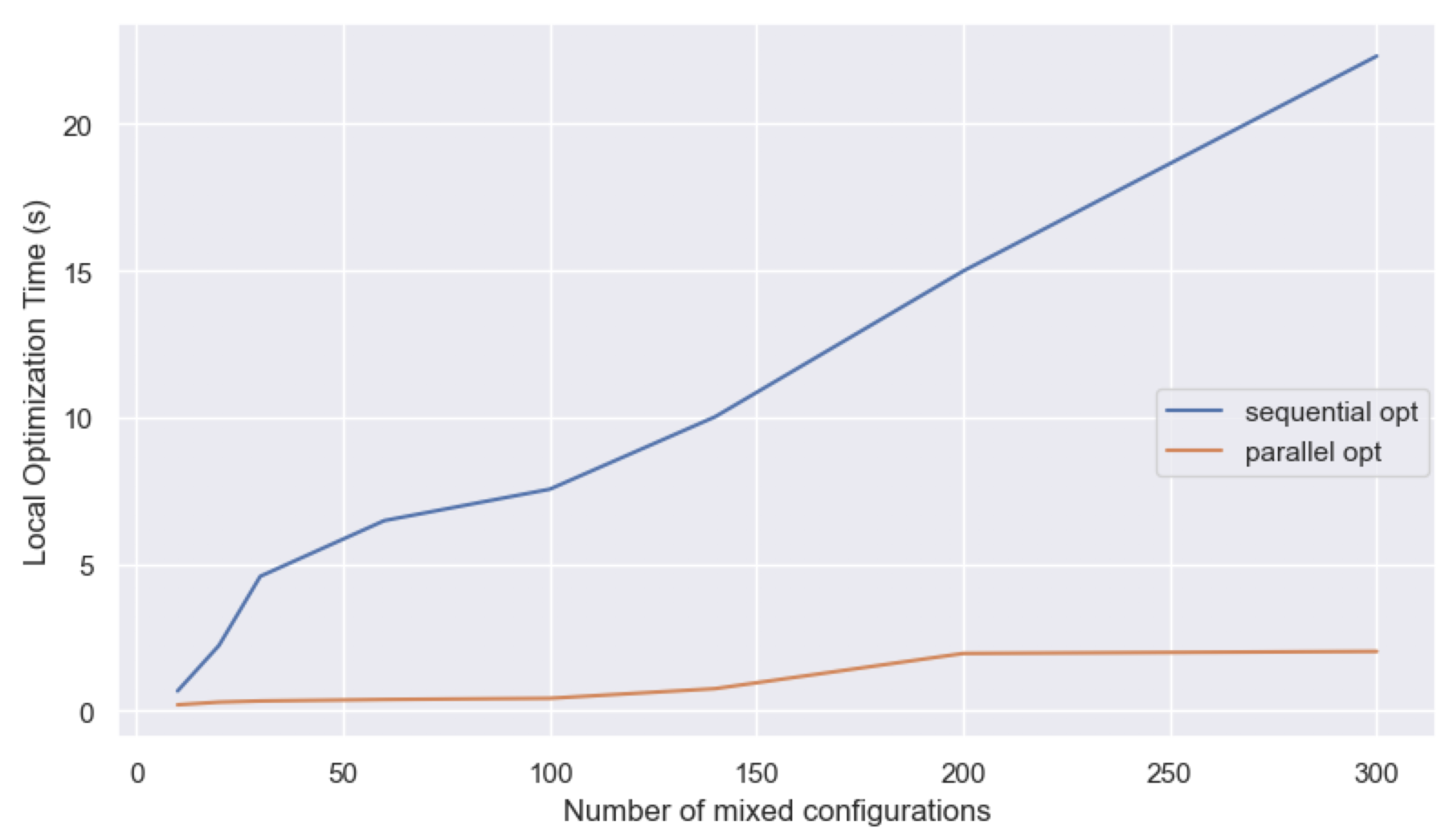
In a real scenario, the number of mixed configurations to be optimized can reach several thousands. For this reason, we introduced the capability to perform local optimizations in parallel. In
Table 5 and
Table 6 we show, respectively, the local sequential optimization times and the local parallel optimization times for mixed configurations. In
Table 4 we can notice that from 5 to 150 mixed configurations, we increase the sequential optimization time from 0.67 to 22.32 in
value. However, by introducing parallel optimization, we are able to remain under 2 s of optimization time for 150 mixed configurations (see
Table 6). The local optimizations are performed in parallel by the aggregator to achieve better performance. As for the local optimization time, the model scales quite well with an increasing number of mixed configurations. The aggregate optimization time is indeed very low; the variation it has with an increasing number of mixed configurations is almost negligible.
In
Figure 21 we can see the different degree of scalability of our systems based on sequential and parallel local optimization of mixed configurations: by allowing parallel optimizations, we can control the optimization times by gaining from a 25% (for the case of 5 mixed configurations) to an 80% for the 300 mixed configuration case.
8. Conclusions
This paper presented the VIRTUS project, in which a prototype of a VPP platform is developed. We tested the scalability of an optimization algorithm used for the management of various distributed resources, with satisfactory results. We also showed that the scalability can be greatly enhanced by the use of parallel optimization.
The project includes several components strongly connected and capable of communicating with each other: (1) several real monitored sites; (2) a simulator to generate profiles of individual plants that can be aggregated in mixed configurations to obtain complex simulated scenarios; (3) an optimization component with different levels of optimization (local, aggregate and at run-time); (4) a market simulator to obtain energy market prices. This design allows for agile testing of new features to be added as the market, the regulatory, and the technological framework change. As shown in the case studies analyzed in the experiments, the work focused on the modeling of aggregation algorithm for managing thousands of loads and microgrid centrally to provide flexibility to the TSO through the balancing markets.
Generally, the strength of a VPP lies in exploiting the potential of the electrical and thermal resources distributed to the customer, thus allowing it to be involved with new business opportunities from a win-win perspective. Through the use of ICT systems, the project intends to provide energy providers with the ability to manage the growing presence of renewable sources, aggregating the flexibility of DERs and supporting conventional generation in the management of the electricity system. The development of the prototype of this project can give rise to interesting synergies to create management and optimization products and value-added services. Currently the system is tested on simulated data and on a single market scenario, but it is meant to be tested on real industrial sites and potentially different market scenarios, which will enhance the impact of the project.
Further development will include the simulation of more complex scenarios, with dynamic market simulations, extreme weather scenarios, and simulation of balancing requests from the TSO. This will allow us to test the communication issues among the components of the platform.
Additionally, since the central optimization module can be considered agnostic with respect to the local DERs that compose the VPP system, we are planning to place the simulated components in a simulated power grid in order to study and analyze the effects of the VPP on distribution networks.
Finally, the financial aspect of running a VPP could be explored, for example, by investigating the optimal bidding strategies on the balancing markets.
Author Contributions
Conceptualization, S.B., F.S., A.D.F., S.M.; methodology, all; software, A.D.F., G.M.; validation, A.D.F., G.M.; formal analysis, all; investigation, all; resources, F.S., S.B., S.M.; data curation, A.D.F., G.M.; writing–original draft preparation, A.D.F., G.M.; writing–review and editing, all; visualization, A.D.F., G.M.; supervision, F.S.; project administration, F.S., S.B.; funding acquisition, F.S., S.B., S.M. All authors have read and agreed to the published version of the manuscript.
Funding
VIRTUS Project, funded by Cassa per i Servizi Energetici e Ambientali (Fund for Energy and Environmental Services—CSEA)—Project code CCSEB_00094.
Data Availability Statement
Conflicts of Interest
The authors declare no conflict of interest.
References
- International Energy Agency (IEA). Global Energy Review 2021; International Energy Agency (IEA): Paris, France, 2021. [Google Scholar]
- Babatunde, O.M.; Munda, J.L.; Hamam, Y. Power system flexibility: A review. Energy Rep. 2020, 6, 101–106. [Google Scholar] [CrossRef]
- Saboori, H.; Mohammadi, M.; Taghe, R. Virtual Power Plant (VPP), Definition, Concept, Components and Types. In Proceedings of the 2011 Asia-Pacific Power and Energy Engineering Conference, Wuhan, China, 25–28 March 2011; pp. 1–4. [Google Scholar] [CrossRef]
- VIRTUal Management of Distributed Energy Resources (VIRTUS) Project. Available online: http://www.virtus-csea.it/ (accessed on 1 March 2021).
- IRENA. Innovation Landscape Brief: Aggregators; International Renewable Energy Agency: Abu Dhabi, United Arab Emirates, 2019. [Google Scholar]
- Burger, S.; Chaves-Ávila, J.P.; Batlle, C.; Pérez-Arriaga, I.J. A review of the value of aggregators in electricity systems. Renew. Sustain. Energy Rev. 2017, 77, 395–405. [Google Scholar] [CrossRef]
- Integrated National Energy and Climate Plan. Available online: https://www.mise.gov.it/images/stories/documenti/it_final_necp_main_en.pdf (accessed on 1 March 2021).
- De Filippo, A.; Lombardi, M.; Milano, M.; Borghetti, A. Robust optimization for virtual power plants. In Proceedings of the Conference of the Italian Association for Artificial Intelligence, Bari, Italy, 14–17 November 2017; pp. 17–30. [Google Scholar]
- Palma-Behnke, R.; Benavides, C.; Aranda, E.; Llanos, J.; Sáez, D. Energy management system for a renewable based microgrid with a demand side management mechanism. In Proceedings of the 2011 IEEE Symposium on Computational Intelligence Applications In Smart Grid (CIASG), Paris, France, 11–15 April 2011; pp. 1–8. [Google Scholar]
- Lombardi, P.; Powalko, M.; Rudion, K. Optimal operation of a virtual power plant. In Proceedings of the IEEE the Power & Energy Society General Meeting, PES’09, Calgary, AB, Canada, 26–30 July 2009; pp. 1–6. [Google Scholar]
- Palensky, P.; Dietrich, D. Demand side management: Demand response, intelligent energy systems, and smart loads. IEEE Trans. Ind. Inf. 2011, 7, 381–388. [Google Scholar] [CrossRef] [Green Version]
- De Filippo, A.; Lombardi, M.; Milano, M. User-aware electricity price optimization for the competitive market. Energies 2017, 10, 1378. [Google Scholar] [CrossRef]
- De Filippo, A.; Lombardi, M.; Milano, M. Non-linear Optimization of Business Models in the Electricity Market. In International Conference on AI and OR Techniques in Constraint Programming for Combinatorial Optimization Problems; Springer: Berlin, Germany, 2016; pp. 81–97. [Google Scholar]
- Reddy, S.S.; Sandeep, V.; Jung, C.M. Review of stochastic optimization methods for smart grid. Front. Energy 2017, 11, 197–209. [Google Scholar] [CrossRef]
- Zhou, Z.; Zhang, J.; Liu, P.; Li, Z.; Georgiadis, M.C.; Pistikopoulos, E.N. A two-stage stochastic programming model for the optimal design of distributed energy systems. Appl. Energy 2013, 103, 135–144. [Google Scholar] [CrossRef]
- Jurković, K.; Pandšić, H.; Kuzle, I. Review on unit commitment under uncertainty approaches. In Proceedings of the IEEE Information and Communication Technology, Electronics and Microelectronics (MIPRO), 2015 38th International Convention, Opatija, Croatia, 25–29 May 2015; pp. 1093–1097. [Google Scholar]
- Hentenryck, P.V.; Bent, R. Online Stochastic Combinatorial Optimization; The MIT Press: Cambridge, MA, USA, 2009. [Google Scholar]
- Zheng, Q.P.; Wang, J.; Liu, A.L. Stochastic Optimization for Unit Commitment, A Review. IEEE Trans. Power Syst. 2015, 30, 1913–1924. [Google Scholar] [CrossRef]
- Zhao, C.; Guan, Y. Unified Stochastic and Robust Unit Commitment. IEEE Trans. Power Syst. 2013, 28, 3353–3361. [Google Scholar] [CrossRef]
- Edwards, R.E.; New, J.; Parker, L.E. Predicting future hourly residential electrical consumption: A machine learning case study. Energy Build. 2012, 49, 591–603. [Google Scholar] [CrossRef]
- Jain, R.K.; Smith, K.M.; Culligan, P.J.; Taylor, J.E. Forecasting energy consumption of multi-family residential buildings using support vector regression: Investigating the impact of temporal and spatial monitoring granularity on performance accuracy. Appl. Energy 2014, 123, 168–178. [Google Scholar] [CrossRef]
- De Filippo, A.; Lombardi, M.; Milano, M. Hybrid Offline/Online Optimization Under Uncertainty. In Proceedings of the 24th European Conference on Artificial Intelligence, ECAI 2020, Santiago de Compostela, Spain, 29 August–5 September 2020. [Google Scholar]
- Weron, R. Electricity price forecasting: A review of the state-of-the-art with a look into the future. IEEE Trans. Power Syst. 2014, 30, 1030–1081. [Google Scholar] [CrossRef] [Green Version]
- Hong, T.; Fan, S. Probabilistic electric load forecasting: A tutorial review. Int. J. Forecast. 2016, 32, 914–938. [Google Scholar] [CrossRef]
- Hong, T.; Pinson, P.; Wang, Y.; Weron, R.; Yang, D.; Zareipour, H. Energy Forecasting: A Review and Outlook. IEEE Open Access J. Power Energy 2020, 7, 376–388. [Google Scholar] [CrossRef]
- Klaboe, G.; Eriksrud, A.L.; Fleten, S.E. Benchmarking time series based forecasting models for electricity balancing market prices. Energy Syst. 2015, 6, 43–61. [Google Scholar] [CrossRef] [Green Version]
- Dimoulkas, I.; Amelin, M.; Hesamzadeh, M.R. Forecasting balancing market prices using Hidden Markov Models. In Proceedings of the 2016 13th International Conference on the European Energy Market (EEM), Porto, Portugal, 6–9 June 2016; pp. 1–5. [Google Scholar]
- Smarter Grid: Empowering SG Market ACtors through Information and Coummunication Technologies. Available online: http://www.smarteremc2.eu/ (accessed on 1 March 2021).
- Australian Gas Light Company VPP. Available online: https://arena.gov.au/projects/agl-virtual-power-plant (accessed on 1 March 2021).
- eTelligence Project. Available online: https://www.energymeteo.com/customers/research_projects/eTelligence.php (accessed on 1 March 2021).
- Fenix Project. Available online: http://www.fenix-project.org/ (accessed on 1 March 2021).
- Binding, C.; Gantenbein, D.; Jansen, B.; Sundström, O.; Bach Andersen, P.; Marra, F.; Poulsen, B.; Træholt, C. Electric vehicle fleet integration in the danish EDISON project—A virtual power plant on the island of Bornholm. In Proceedings of the IEEE PES General Meeting, Minneapolis, MN, USA, 25–29 July 2010; pp. 1–8. [Google Scholar]
- VPP4ISLANDS Project. Available online: https://vpp4islands.eu/ (accessed on 1 March 2021).
- De Filippo, A.; Lombardi, M.; Milano, M. Methods for off-line/on-line optimization under uncertainty. In Proceedings of the Twenty-Seventh International Joint Conference on Artificial Intelligence (IJCAI-18), Stockholm, Sweden, 13–19 July 2018; pp. 1270–1276. [Google Scholar]
- Ferrari, L.; Esposito, F.; Becciani, M.; Ferrara, G.; Magnani, S.; Andreini, M.; Bellissima, A.; Cantù, M.; Petretto, G.; Pentolini, M. Development of an optimization algorithm for the energy management of an industrial Smart User. Appl. Energy 2017, 208, 1468–1486. [Google Scholar] [CrossRef]
- Regulation on the Modalities for the Creation, Qualification and Management of Authorised Mixed Virtual Units to the Dispatching Services Market, Art. 10, Par. 1, Lett. g. Available online: https://www.terna.it/it/sistema-elettrico/pubblicazioni/news-operatori/dettaglio/uvam-del-70-2021 (accessed on 1 March 2021).
- Kaplanis, S.; Kaplani, E. A model to predict expected mean and stochastic hourly global solar radiation I(h;nj) values. Renew. Energy 2007, 32, 1414–1425. [Google Scholar] [CrossRef]
- Espinosa, A.; Ochoa, L. Dissemination Document a Low Voltage Networks Models and Low Carbon Technology Profiles; Technical Report; University of Manchester: Manchester, UK, 2015. [Google Scholar]
- Massucco, S.; Mosaico, G.; Saviozzi, M.; Silvestro, F. A Hybrid Technique for Day-Ahead PV Generation Forecasting Using Clear-Sky Models or Ensemble of Artificial Neural Networks According to a Decision Tree Approach. Energies 2019, 12, 1298. [Google Scholar] [CrossRef] [Green Version]
- Ogunjuyigbe, A.; Ayodele, T.; Akinola, O. Optimal allocation and sizing of PV/Wind/Split-diesel/Battery hybrid energy system for minimizing life cycle cost, carbon emission and dump energy of remote residential building. Appl. Energy 2016, 171, 153–171. [Google Scholar] [CrossRef]
- Tulabing, R.; Yin, R.; DeForest, N.; Li, Y.; Wang, K.; Yong, T.; Stadler, M. Modeling study on flexible load’s demand response potentials for providing ancillary services at the substation level. Electr. Power Syst. Res. 2016, 140, 240–252. [Google Scholar] [CrossRef] [Green Version]
- Mosaico, G.; Saviozzi, M.; Silvestro, F.; Bagnasco, A.; Vinci, A. Simplified State Space Building Energy Model and Transfer Learning Based Occupancy Estimation for HVAC Optimal Control. In Proceedings of the 2019 IEEE 5th International forum on Research and Technology for Society and Industry (RTSI), Florence, Italy, 9–12 September 2019; pp. 353–358. [Google Scholar]
- De Mello Martins, P.B.; Nascimento, V.B.; de Freitas, A.R.; e Silva, P.B.; Pinto, R.G.D. Industrial Machines Dataset for Electrical Load Disaggregation. 2018. Available online: https://ieee-dataport.org/open-access/industrial-machines-dataset-electrical-load-disaggregation (accessed on 1 March 2021).
- Conte, F.; D’Agostino, F.; Pongiglione, P.; Saviozzi, M.; Silvestro, F. Mixed-Integer Algorithm for Optimal Dispatch of Integrated PV-Storage Systems. IEEE Trans. Ind. Appl. 2019, 55, 238–247. [Google Scholar] [CrossRef]
- Resolution 300/2017/R/eel, Updated with Resolutions 372/2017/R/eel, 422/2018/R/eel and 70/2021/R/eel of the Italian Regulatory Authority for Energy, Networks and Environment (ARERA). Available online: https://www.arera.it/it/docs/17/300-17.htm (accessed on 1 March 2021).
- Netlogo. Available online: http://ccl.northwestern.edu/netlogo/ (accessed on 1 March 2021).
- Gurobi Solver Page. Available online: http://www.gurobi.com/ (accessed on 1 March 2021).
Figure 1.
A visual representation of a Virtual Power Plant and its available DERs.
Figure 1.
A visual representation of a Virtual Power Plant and its available DERs.
Figure 2.
A VPP distributed architecture.
Figure 2.
A VPP distributed architecture.
Figure 3.
A graphical interface of a virtual unit composed by heterogeneous plants on LIBRA platform.
Figure 3.
A graphical interface of a virtual unit composed by heterogeneous plants on LIBRA platform.
Figure 4.
Example of baseline for a plant on LIBRA platform.
Figure 4.
Example of baseline for a plant on LIBRA platform.
Figure 5.
Example of available data for a component on LIBRA platform.
Figure 5.
Example of available data for a component on LIBRA platform.
Figure 6.
Different Levels of Optimization.
Figure 6.
Different Levels of Optimization.
Figure 7.
Examples of PODs.
Figure 7.
Examples of PODs.
Figure 8.
Local POD Optimization.
Figure 8.
Local POD Optimization.
Figure 9.
Four classes of load in VPP optimization problem. Blue profile is the uncontrolled profile; red profile is the profile with implemented control. (a) L1 (sheddable load); (b) L2 (shiftable and sheddable load); (c) L3 (shiftable load with daily conservation); (d) L4 (non-controllable load). Please note that in (d) the two profiles completely coincide.
Figure 10.
Central Aggregator Optimization.
Figure 10.
Central Aggregator Optimization.
Figure 11.
General Structure and Communication.
Figure 11.
General Structure and Communication.
Figure 12.
Probabilistic model for price of upward regulation in center north zone.
Figure 12.
Probabilistic model for price of upward regulation in center north zone.
Figure 13.
Probabilistic model for quantity of downward regulation in north zone.
Figure 13.
Probabilistic model for quantity of downward regulation in north zone.
Figure 14.
VPP graphical interface in Netlogo.
Figure 14.
VPP graphical interface in Netlogo.
Figure 15.
(right) Baseline for PV setting. (left) Baseline for WIND setting.
Figure 15.
(right) Baseline for PV setting. (left) Baseline for WIND setting.
Figure 16.
(right) Baseline for LOAD1 setting. (left) Baseline for LOAD3 setting.
Figure 16.
(right) Baseline for LOAD1 setting. (left) Baseline for LOAD3 setting.
Figure 17.
(Up) Case study 1 setting. (Down) Case study 1 results.
Figure 17.
(Up) Case study 1 setting. (Down) Case study 1 results.
Figure 18.
(Up) Case study 2 setting. (Down) Case study 2 results.
Figure 18.
(Up) Case study 2 setting. (Down) Case study 2 results.
Figure 19.
(Up) Case study 3 setting. (Down) Case study 3 results.
Figure 19.
(Up) Case study 3 setting. (Down) Case study 3 results.
Figure 20.
(Up) Case study 4 setting. (Down) Case study 4 results.
Figure 20.
(Up) Case study 4 setting. (Down) Case study 4 results.
Figure 21.
Sequential/parallel Local Optimization.
Figure 21.
Sequential/parallel Local Optimization.
Table 1.
Components currently modeled in the VPP.
Table 1.
Components currently modeled in the VPP.
| Name | Type | Reference |
|---|
| PV | Generator | [39] |
| Wind | Generator | [41] |
| Markovian Binary Load | Load | - |
| HVAC | Load | [42] |
| Industrial | Load | [43] |
| Battery | Load/Generator | [44] |
| Intelligent POD | Load/Generator | [35] |
Table 2.
Mixed configurations and components based on scenario 5.
Table 2.
Mixed configurations and components based on scenario 5.
| Conf | RES | BESS | L1 (Sheddable) | L2 (Shiftable/ Sheddable) | L3 (Shiftable/ Daily Cons) | L4 (Non-Controllable) |
|---|
| 1 | X | X | X | | | X |
| 2 | X | X | | X | X | |
| 3 | X | | | X | | |
| 4 | X | X | | X | X | |
| 5 | X | X | X | | | |
| 6 | X | | X | | | X |
Table 3.
Specific plants included in the case studies of this paper.
Table 3.
Specific plants included in the case studies of this paper.
| Name | Type | Nominal Power [kW] | Details |
|---|
| PV1 | PV | 20 | - |
| PV2 | PV | 400 | - |
| WIND1 | Wind | 1000 | - |
| WIND2 | Wind | 2000 | - |
| LOAD1 | Load L1 | 1 | Markov Binary Load |
| LOAD2 | Load L2 | 100 | HVAC |
| LOAD3 | Load L3 | 10,000 | Industrial Load |
| LOAD4 | Load L4 | 7 | Industrial Load |
| BESS1 | BESS | 30 | 30 kWh capacity |
| BESS2 | BESS | 70 | 70 kWh capacity |
Table 4.
Comparison number of plants/time for the 4 case study simulations.
Table 4.
Comparison number of plants/time for the 4 case study simulations.
| Simulation | # of Single Plants | # of Mixed Configurations | Local Optimization Time () s | Local Optimization Time () s | Aggregation Time () s | Aggregation Time () s |
|---|
| case study 1 | 100 | 50 | 7.45 | 0.92 | 2.35 | 0.55 |
| case study 2 | 120 | 50 | 7.77 | 0.99 | 2.97 | 0.51 |
| case study 3 | 100 | 50 | 7.62 | 1.01 | 2.45 | 0.50 |
| case study 4 | 120 | 50 | 7.81 | 1.05 | 3.05 | 0.55 |
Table 5.
Comparison number of plants/time for different size of simulation (case study 4) with local sequential optimization.
Table 5.
Comparison number of plants/time for different size of simulation (case study 4) with local sequential optimization.
| Simulation | # of Single Plants | # of Mixed Configurations | Local Opt (Seq) Time () s | Local Opt (Seq) Time () s | Aggregation Opt Time () s | Aggregation Opt Time () s |
|---|
| case study 4 | 5 | 5 | 0.67 | 0.12 | 0.05 | 0.01 |
| case study 4a | 10 | 10 | 2.22 | 0.25 | 0.52 | 0.10 |
| case study 4b | 15 | 15 | 4.58 | 0.74 | 0.77 | 0.15 |
| case study 4c | 30 | 30 | 6.48 | 0.81 | 0.97 | 0.22 |
| case study 4d | 50 | 50 | 7.55 | 0.88 | 1.86 | 0.55 |
| case study 4e | 70 | 70 | 10.02 | 0.90 | 2.23 | 0.80 |
| case study 4f | 100 | 100 | 14.99 | 0.90 | 3.44 | 0.92 |
| case study 4g | 150 | 150 | 22.32 | 1.15 | 4.21 | 1.01 |
Table 6.
Comparison number of plants/time for different size of simulation (case study 4) with local parallel optimization.
Table 6.
Comparison number of plants/time for different size of simulation (case study 4) with local parallel optimization.
| Simulation | # of Single
Plants | # of Mixed
Configurations | Local Opt (par)
Time () s | Local Opt (par)
Time () s | Aggregation Opt
Time () s | Aggregation Opt
Time () s |
|---|
| case study 4 | 5 | 5 | 0.20 | 0.02 | 0.05 | 0.01 |
| case study 4a | 10 | 10 | 0.29 | 0.05 | 0.52 | 0.10 |
| case study 4b | 15 | 15 | 0.33 | 0.04 | 0.77 | 0.15 |
| case study 4c | 30 | 30 | 0.38 | 0.01 | 0.97 | 0.22 |
| case study 4d | 50 | 50 | 0.42 | 0.04 | 1.86 | 0.55 |
| case study 4e | 70 | 70 | 0.75 | 0.02 | 2.23 | 0.80 |
| case study 4f | 100 | 100 | 1.95 | 0.09 | 3.44 | 0.92 |
| case study 4g | 150 | 150 | 2.02 | 0.09 | 4.21 | 1.01 |
| Publisher’s Note: MDPI stays neutral with regard to jurisdictional claims in published maps and institutional affiliations. |
© 2021 by the authors. Licensee MDPI, Basel, Switzerland. This article is an open access article distributed under the terms and conditions of the Creative Commons Attribution (CC BY) license (https://creativecommons.org/licenses/by/4.0/).


 and
and 


