Online Measurement Error Detection for the ElectronicTransformer in a Smart Grid

Abstract

With the development of smart power grids, electronic transformers have been widely used to monitor the online status of power grids. However, electronic transformers have the drawback of poor long-term stability, leading to a requirement for frequent measurement. Aiming to monitor the online status frequently and conveniently, we proposed an attention mechanism-optimized Seq2Seq network to predict the error state of transformers, which combines an attention mechanism, Seq2Seq network, and bidirectional long short-term memory networks to mine the sequential information from online monitoring data of electronic transformers. We implemented the proposed method on the monitoring data of electronic transformers in a certain electric field. Experiments showed that our proposed attention mechanism-optimized Seq2Seq network has high accuracy in the aspect of error prediction.

1. Introduction

Currently, modern power grids are experiencing intensification and informatization. Owing to the rapid construction of intelligent power grids, a number of electronic transformers (ETs) are used in applications [1]. An ET consists of sensors and signal processing units, used to measure electronic current and voltage. Compared with traditional magnetic transformers, it has more advantages, such as low cost, high bandwidth, good insulation performance, and adapting to the development trend of digitalization and intelligence. However, the current problem with ETs is their poor long-term stability [2]. As a typical electrical measuring device, online monitoring and the evaluation of measurement error status of electronic transformers are of great importance for the safety and reliability of the power grid.

Due to technical limitations, the evaluation methods for ET error status are mainly divided into three types: the first one is regularly checking transformers that are running [3]. It uses high-accuracy transformers to connect with the measured transformers loop, and then measures the ratio and angular difference of the tested transformers. However, the operation is very complicated, which requires quitting the tested transformers and ceasing the power line. In addition, examining the error state of transformers regularly is only a short-term procedure, which is unsuitable to implement online evaluation and monitoring of the long-term operational status of transformers. Therefore, it cannot accurately perceive the error change of transformers when the grid runs, and it is difficult to discover its potential error change trend. The second method is to run the high-standard transformers and measure transformers in parallel and monitor the error on the measured transformers for a long time [4,5], which realizes the long-term error state monitoring of transformers. However, it still has the weakness of low traceability of the standard transformer. To complete the accurate monitoring of measured transformers, reliable standard transformers are required so standard transformers also need to be checked regularly. At present, the access and exit of standard transformers require line outage under test, which is quite complicated. Therefore, the long-term parallel operation of standard transformers also brings more complex fixing problems. Additionally, the long-term integration of standard transformers into the power system operation also affects the operating parameters of the grid, increasing the risk for grid security and stability, which decreases the reliability of the power grids. Therefore, it is difficult to achieve this method in production [6,7,8]. The third method is based on data-driven and model analysis of the electronic transformer’s condition assessment method. The former is mainly aimed at the evaluation of the variation of transformers but not the long-term and gradual error which is an important performance evaluation index for electronic transformers. Additionally, the latter method must rely on accurately physical and mathematical models [9], which is not suitable in field engineering applications.

In summary, existing methods only support short-term online verification of transformers, which is far from ensuring the performance of transformers [10,11,12]. Therefore, existing methods cannot satisfy the intelligent requirements of the development of smart grids for equipment maintenance [13,14]. There are still several shortcomings in the process of evaluating and monitoring transformers, as follows. (1) Currently, the research is mainly on offline periodic maintenance and short-term online verification, which cannot complete long-term online monitoring and evaluation; (2) there are few studies aimed at the long-term online monitoring of the current transformer status and the accurate acquisition technology of the primary line voltage and current signals; (3) how to accurately evaluate the operating state of the transformer without high-precision standard transformers that are involved in extracting and judging the feature quantities of the operating characterization transformers; (4) how to ensure the accuracy of stateful inspection and evaluation results, where the difficulty lies in the design and implementation of sampling testing methods; (5) it is difficult to accurately evaluate the error state of transformers without exemplary transformers, and how to separate and distinguish the change in the transformer error caused by the grid fault and the transformer error change caused by the transformers’ failure.

Based on the evaluation of the error state of electronic transformers, we proposed an attention mechanism-optimized sequence-to-sequence (Seq2Seq) network to predict the error state of transformers that are used for fault location and early warning of transformers. In Section 1.1, we review the long short-term memory networks and Seq2Seq model. Then, we present the attention mechanism-optimized Seq2Seq network for prediction in Section 1.2. In Section 2, we implement extensive experiments to illustrate the effectiveness of the proposed algorithm. Finally, we draw a conclusion in Section 3.

1.1. Related Works

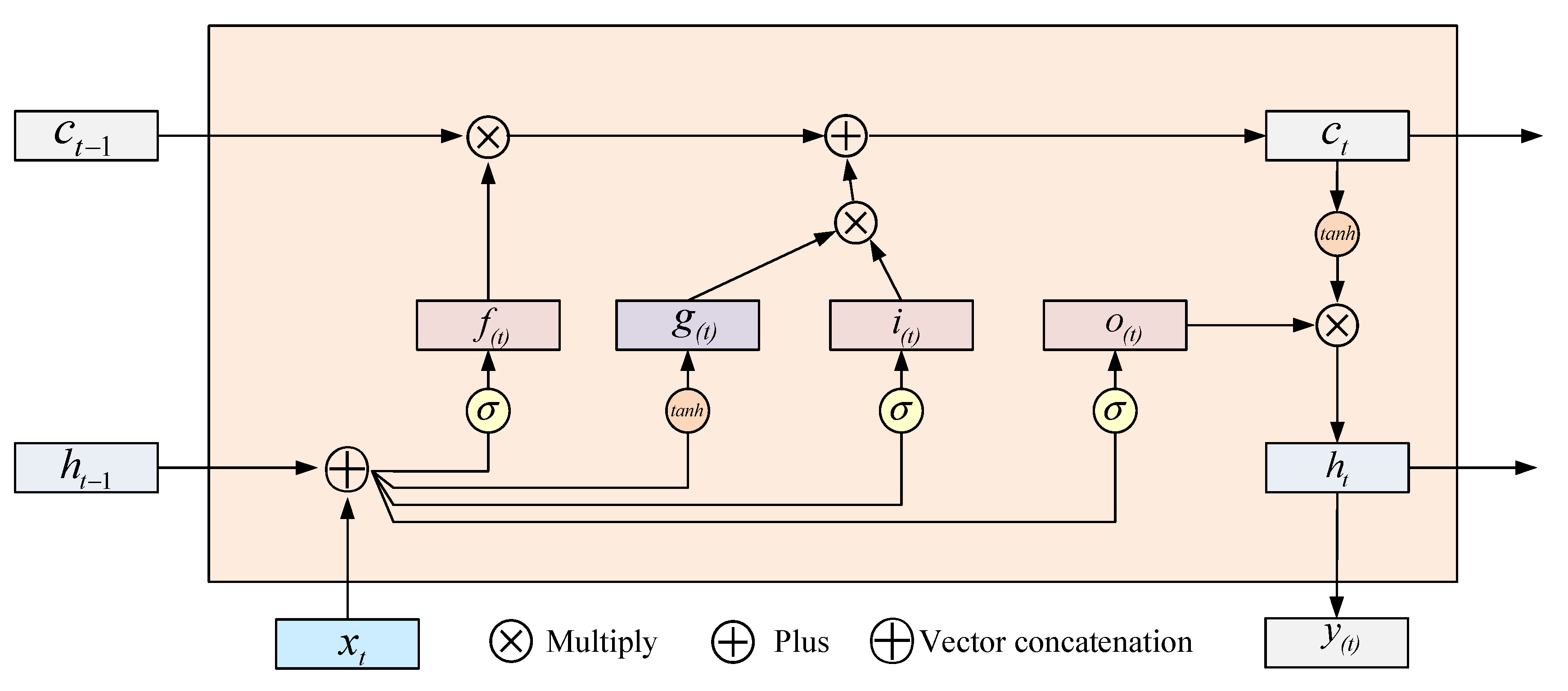
1.1.1. Long Short-Term Memory (LSTM) Network

LSTM is a kind of cyclic neural network, which aims to solve the problem of long-term dependence in the time series model. In all the cyclic neural network models, there is processing of timing sequence information. The essence of LSTM is an improvement based on the basic cyclic neural network structure. Three important gate control functions are reintroduced into the memory unit module, which are named the forget gate [15], input gate, and output gate. The standard network structure of LSTM is shown in Figure 1 below.

In the forward propagation process of the LSTM, information preservation and interaction are controlled through the three gate structures of the memory unit of the hidden layer.

(1)

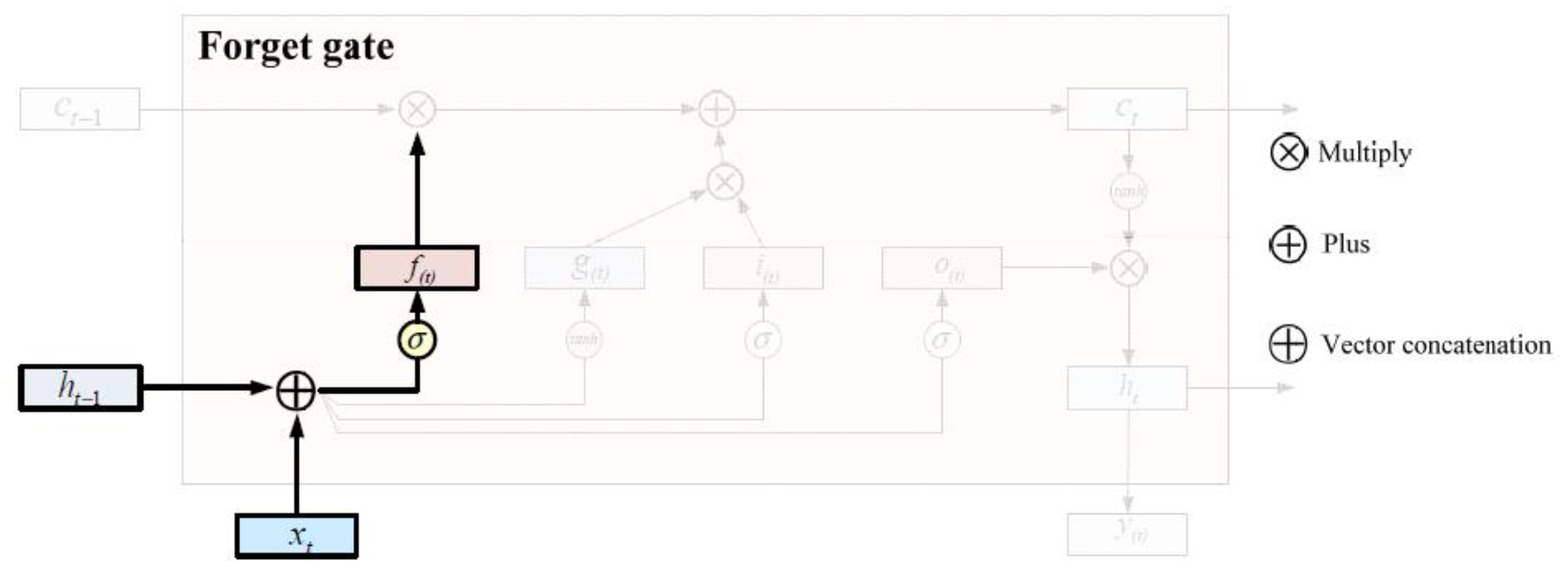
Forget gate $f_t$: The forget gate is used to control the proportion of input information, and when the time sequence information passes through the forget gate, part of the information is discarded so that the time span of each batch of data is the same and the data volume is not too large. This ratio control outputs a value between 0 and 1 through the sigmoid layer, with 0 representing “complete abandonment” and 1 representing “complete retention”. The implementation diagram of the forget door is shown in Figure 2.

The calculation formula of the forget gate is as follows:

$$f_t=\sigma \left(W_f·\left[h_{t-1},x_t\right]+b_f\right)$$

(1)

where:

$h_{t-1}$ denotes the output at time of $t-1$, $x_t$ denotes the information in the network at the time of $t$, $\sigma$ is the sigmoid function, $W_f$ is the weight matrix for the forget gate, and $b_f$ is the bias term for the forget gate.

(2)

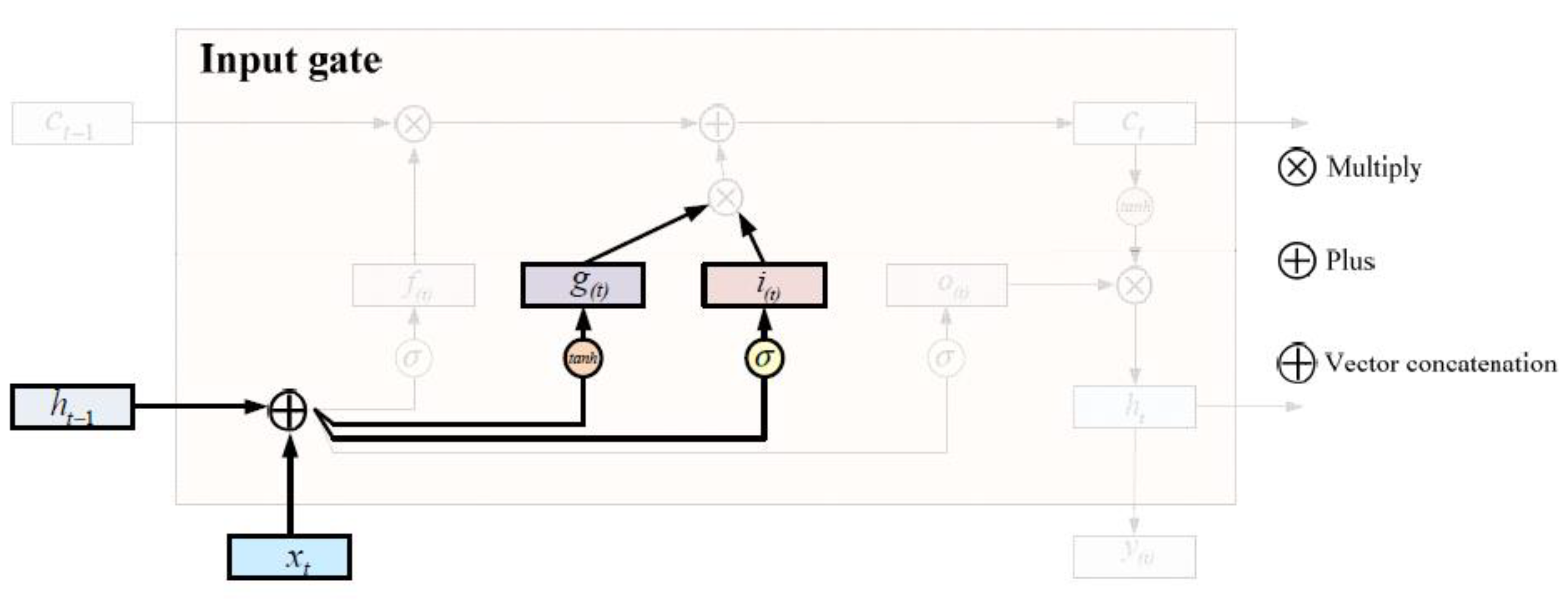
Input gate $i_t:$ The input gate controls the input process of the current moment information. This process includes the input gate completing the updating of the current moment information, and at the same time superimposes the input of a moment on the hidden layer to the current state. The input gate function includes a sigmoid function. The implementation diagram of the input gate is shown in Figure 3.

The superposition process of the output and current input at one time on the hidden layer is shown as follows:

$$i_t=\sigma \left(W_i·\left[h_{t-1},x_t\right]+b_i\right)$$

(2)

where:

$h_{t-1}$ denotes the output at time of $t-1$, $x_t$ denotes the information in the network at time of $t$, $\sigma$ is the sigmoid function, $W_i$ is the weight matrix for the input gate, and $b_i$ is the bias term for the input gate.

The calculation method for updating the current moment information is shown in the following formula:

$${\tilde{C}}_t=\tan \mathrm{h}\left(W_C\left[h_{t-1},x_t\right]+b_C\right)$$

(3)

where:

${\tilde{C}}_t$ is the candidate for memory unit, $h_{t-1}$ denotes the output at time of $t-1$, $x_t$ denotes the information in the network at time of $t$, $W_C$ is the weight matrix for the cell, and $b_C$ is the bias term for the cell.

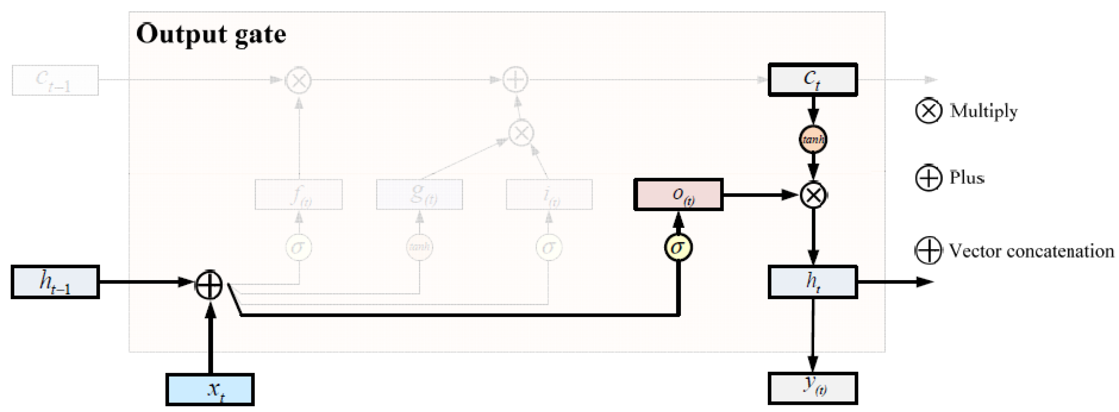
At the current moment of $t$, the memory unit of the hidden layer completes the multiplication of information and can realize the memory output unit $C_t$ through the joint action of the forget gate and the input gate. The output calculation formula is shown in the following formulation:

$$C_t=f_t\times C_{t-1}+i_t\times {\tilde{C}}_t$$

(4)

where $f_t$ is the output of the forget gate, $i_t$ is the output of the input gate, $C_{t-1}$ is the output of the cell at time of t − 1, and ${\tilde{C}}_t$ is the candidate for the memory unit.

(3)

Output gate $O_t:$ The output gate function controls the output information and the timing information returned to the hidden layer before the memory unit information is output. By using the output gate, the state is updated, while the state of h_t−1 is retained in the time unit operating under the hidden layer. The implementation diagram of the output gate is shown in Figure 4 below.

The calculation formula of the output gate output is shown in the following formulation:

$$O_t=\sigma \left(W_0·\left[h_{t-1},x_t\right]+b_0\right)$$

(5)

where $W_O$ is the weight matrix for the output gate and $b_O$ is the bias term for the output gate. $h_t$ information returned to the hidden layer is computed as follows:

$$h_t=O_t\times \tan \mathrm{h}\left(C_t\right)$$

(6)

where $O_t$ is the output of the output gate, $C_t$ is the output of the cell at time of t.

In this way, we get the information returned to the hidden layer.

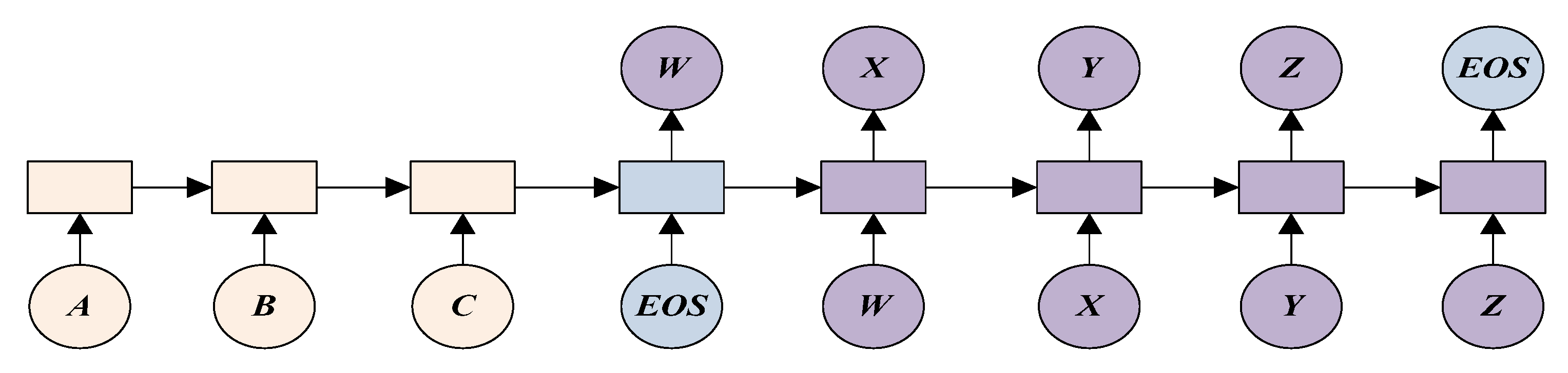
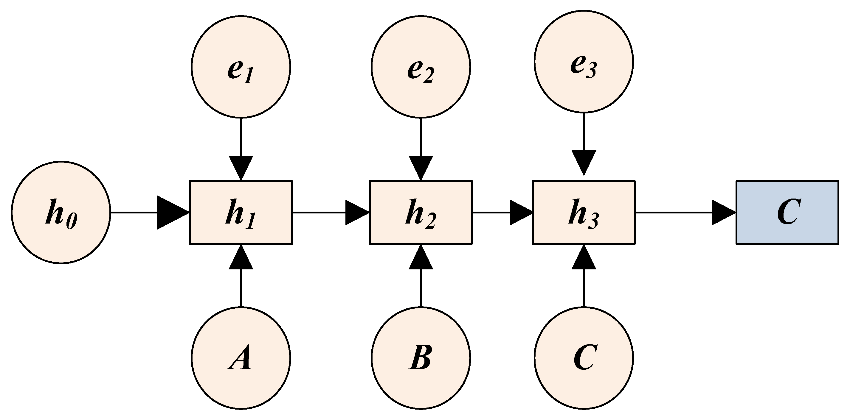
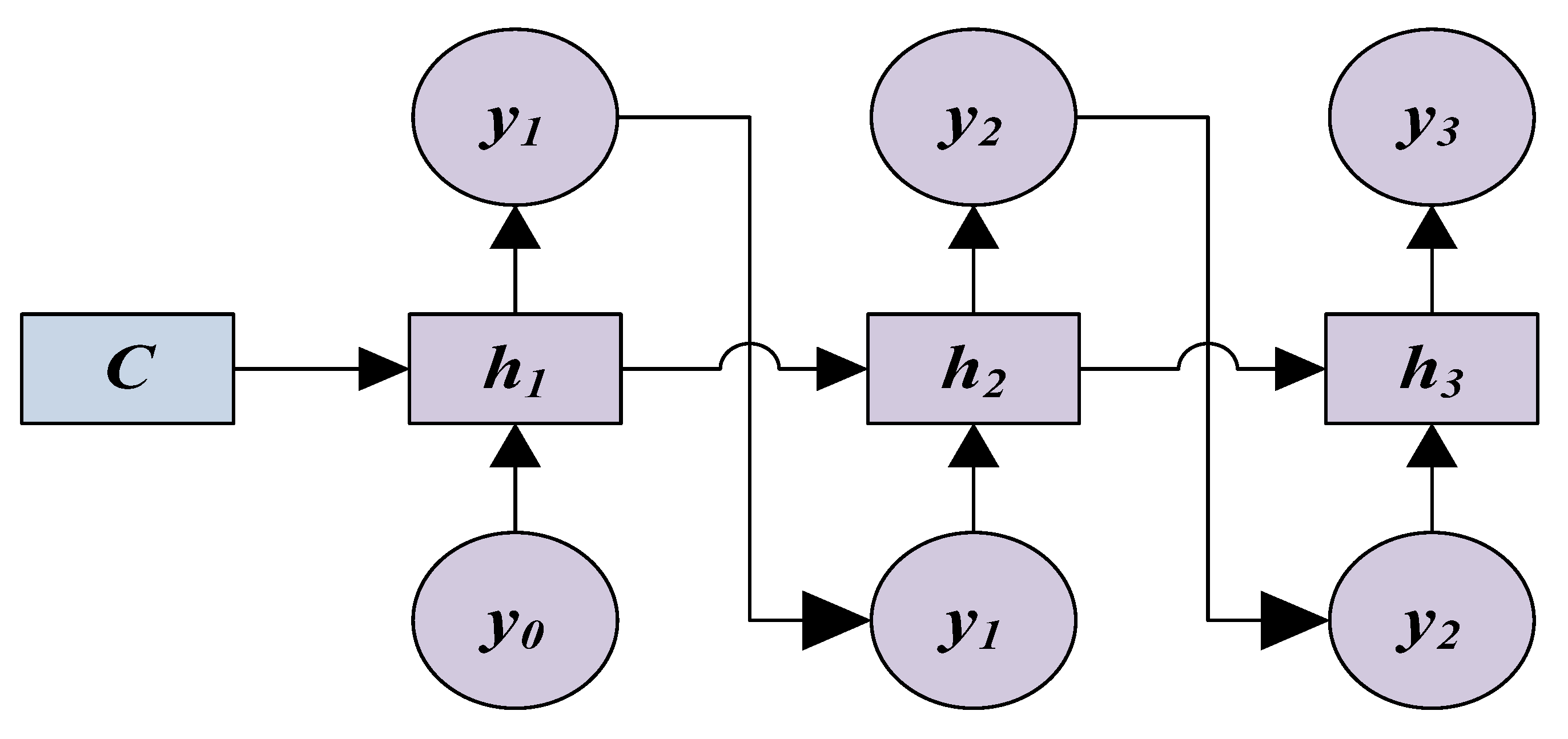
1.1.2. Seq2Seq Network Model

The Seq2Seq network model is also a kind of cyclic neural network, which can be used to deal with sequence prediction problems. It is often widely used in text abstracts, question answering systema, and other fields. The Seq2Seq network model structure for machine translation is shown in Figure 5.

In Figure 5, each rectangular block contains a neural network like LSTM. It can be observed from the above structure diagram that the input of the model to the output of the model is a complete stream, in which ABC is the input of the model encoder part. After that, the sign “end of sentence” (EOS) in the input indicates the termination of the sentence. Then, WXYZ is the input and output of the sequential models in the decoder part. The output state of the last hidden layer in the encoder part is compressed into the expression of fixed dimension word vectors of a specified size, and then the expression of the fixed dimension word vectors is taken as the input of the first hidden layer in the decoder part. The advantage is that the encoder part and decoder part can be regarded as a linear work flow. It is mentioned in [16] that if the model receives input in the order of CBA for calculation, the prediction performance of the model can be improved to some extent because the distance between A and X becomes smaller. The structure diagram of the encoder part is shown in Figure 6, which corresponds to the left part of Figure 5.

From Figure 6 above, we can see that the encoder section [17] is composed of several stacked long short-term memory network units, each of the LSTM cells accepts the input of a single element from the input sequence, and each LSTM neural unit propagates the collected information about the element at this time forward to the next LSTM neural unit through calculation. The calculation formula of the state of each hidden layer is shown in the following formula:

$$h_t=f\left(W^{\left(hh\right)}{h}_{t-1}+W^{\left(hx\right)}{x}_t\right)$$

(7)

where:

$h_t$ is the current hidden layer state,

$W$ is the network weight,

$h_{t-1}$ is the previous hidden layer state,

$x_t$ is the input vector of the current hidden layer.

The structure of the decoder model is shown in Figure 7 below:

As can be seen from Figure 7, the decoder section is also several stacked LSTM network units. The LSTM unit of each time step receives the output of the previous LSTM unit and the state of the previously hidden layer. Candidate symbols are obtained through an activation function and softmax layer, and the one with the highest probability is selected as the output of the current time step.

$$h_t=f\left(W^{\left(hh\right)}{h}_{t-1}\right)$$

(8)

where:

$h_t$ is the current hidden layer state,

$W$ is the network weight,

$h_{t-1}$ is the previous hidden layer state.

$$y_t=\mathrm{softmax}\left(W^S{h}_t\right)$$

(9)

The output value of the output time step is computed by using the hidden layer state of the current time step and the corresponding weight.

1.2. Construction of Prediction Model Based on Optimized Neural Network

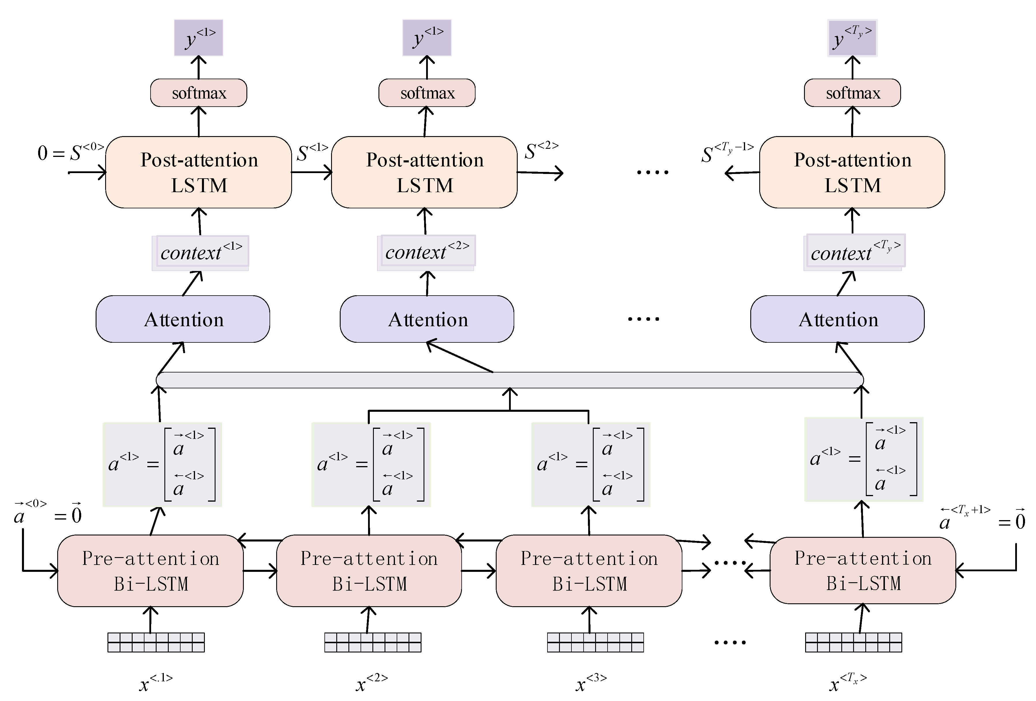
1.2.1. Attention Mechanism (AM)

When analyzing time series data, the characteristics of each element in the sequence should be calculated. When we extract information from sequence data, we need to pay attention to the characteristics of the entire sequence, while simply adding or averaging the features of each element may decrease the independence of elements in the input sequence. Therefore, the attention mechanism needs to be introduced into the model [18,19,20,21].

The introduction of the attention mechanism can also address the limitations of the model’s long-term dependency and lead to efficient usage of memory during computation. As an intermediate layer between the encoding part and decoding part, the attention mechanism aims to capture information from the tag sequence related to the sentence content [22].

The attention mechanism-based network model first computes a set of attention weights and creates a combination of weights by multiplying the vector output by the encoder. The calculated results should contain information about specific parts of the input sequence to help the decoder select the correct representation for the output. Therefore, the decoder can use different parts of the encoder sequence as the context until all sequences are decoded [23]. The framework of the attention mechanism is displayed in Figure 8.

Unlike the encode–decode model, which uses the same context vector for each hidden layer state of the decoder part, the attention mechanism computes a vector $C_t$ and an output $y_t$ for each time step t in the decoding stage [24]. The corresponding calculation formula is shown as follows:

$$C_t={\displaystyle \sum }_{j=1}^T{a}_{tj}{h}_j$$

(10)

where $h_j$ is the hidden layer state of input vector $x_j$, and $a_{tj}$ is the weight of $h_j$ prediction $y_t$. Vector $C_t$ is also known as the expected attention vector and can usually be calculated by a softmax function, as follows:

$${\alpha }_{ij}\frac{\exp \left(e_{ij}\right)}{{{\displaystyle \sum }}_{k=1}^{T}exp\left(e_{ij}\right)}$$

(11)

$$e_{ij}=attentionScore\left(S_{i-1},h_j\right)$$

(12)

Among them, the attentionScore function can select the hidden state of the decoding part and the hidden state of the encoding part to calculate a score used to calculate the weight.

1.2.2. Construction of Seq2Seq Model

Based on the basic introduction of the AM above, the introduction of the attention mechanism into the Seq2Seq network model is expected to reveal the potential relationship between sequence data [16,25], so as to improve the prediction accuracy. In the Seq2Seq model, circulating neural networks are generally used in the process of encoding, such as LSTM and a gate recurrent unit (GRU) [26]. In this study, the encoding and decoding stages used bidirectional LSTM [27]. The online operation state prediction of the transformer is based on the time series. The standard circulating neural network often ignores the future context information when dealing with the problems in the time series. If the network can access the past or future time step context information, it is beneficial to network traffic prediction [28,29]. To solve the above problem, a delay is added between the input and the target to add future information of time frame M together to predict the output result of the current time step. Theoretically speaking, the size of M can be increased to capture all information available for current time step prediction in the future. If M is adjusted to be too large, the result of network traffic prediction will be worse. This is because the network model focuses on so much input information that the joint modeling ability of prediction declines. Therefore, the size of M should be adjusted manually during the experiment. Although the introduction of the M time frame in the model is beneficial, the context information of future time steps cannot be obtained, and the training and prediction task of the network model is inefficient due to the manual adjustment of the size of M. Therefore, the network model selected in the process of encoding in this study was the bidirectional LSTM [30,31].

Bidirectional LSTM (BLSTM) is similar in network structure to LSTM networks because it is constructed with LSTM units. The special feature of BLSTM networks is that they improve long-term dependence without retaining redundant context information. Different from LSTM networks, the BLSTM has two network layers that propagate forward in two parallel directions. The forward and back propagation modes of each layer are similar to the basic neural network propagation mode. Meanwhile, these two network layers carry all the information in the two directions before and after the sequence [32,33]. Therefore, the corresponding formula is adjusted as follows:

$$h_{f_t}=H\left(W_{x{h}_f}{x}_t+W_{h_f{h}_f}{h}_{f_{t-1}}+b_{h_f}\right)$$

(13)

$$h_{b_t}=H\left(W_{x{h}_b}{x}_t+W_{h_b{h}_b}{h}_{b_{t-1}}+b_{h_b}\right)$$

(14)

where $h_f\in R^d$ represents the output vector of the forward neural network layer, $h_b\in R^d$ represents the reverse neural network layer. Different from the LSTM, the final output result of the BLSTM is the combination of the two parts of $y_t=\left[h_{f_t},h_{b_t}\right]$, $y_t\in R^{2d}$.

The structure of the Seq2Seq network model optimized by AM is shown in Figure 9 below:

The bottom half of Figure 9 is the encoder part of the model, and the bottom is a model made by the stacked BLSTM with a length of $T_x$. In this paper, each BLSTM unit is called Pre_attention Bi_LSTM. Its output is represented by $a^{\langle t\rangle }$, which means

$$a^{\langle t\rangle }=\left[{\overrightarrow{a}}^{\langle t\rangle };{\overleftarrow{a}}^{\langle t\rangle }\right]$$

It combines the activation value of the forward propagation of BLSTM with the activation value of backward propagation and then puts the output of $a^{\langle t\rangle }$ and the decoder of the previous time step together for the calculation of the attention mechanism, to obtain the context variable $contex{t}^{\langle t\rangle }$ of each time step. The upper part of Figure 9 is the decoding part. The prediction result of this time step is obtained by inputting the hidden layer state of the previous time step and the context variable $contex{t}^{\langle t\rangle }$ of the current time step into the BLSTM unit of the decoder.

2. Experiment

2.1. Experimental Environment and Data Set

The experiment was carried out with the simulated monitoring data of a capacitor voltage transformer (CVT) in an electric field. The schematic diagram of the CVT is shown in Figure 10. C1 and C2 are the high-voltage capacitance and medium-voltage capacitance of the capacitor voltage divider. The magnetic unit consists of intermediate transformer T1, compensation reactor Z, damping device D, and overvoltage protection device G. After the CVT is connected with the high-voltage system, the capacitor voltage divider transforms the primary high-voltage signal into a lower intermediate-voltage signal, which reduces the insulation requirements of the magnetic unit, and then transforms the intermediate transformer into the required secondary small signal, which is used for metering, measurement and control, protection, communication, and other applications. The secondary output of the CVT has several windings according to different demands, of which laln (2a2n, 3a3n) is the main secondary winding terminal and dadn is the residual voltage winding terminal.

“Amplitude” is extracted from 15 test points: “main variant I group A phase”, “main variant I group B phase”, “main variant I group C phase”, “main variant II group A phase”, “main variant II group B phase”, “main variant II group C phase”, “main variant III group A phase”, “main variant III group B phase”, “main variant III group C phase”, “5449 Line A phase”, “5449 Line B phase”, “5449 Line C phase”, “5450 Line A phase”, “5450 Line B phase”, “5450 Line C phase”. Since the “frequency” is consistent, there are a total of 16 characteristic dimensions, and according to the 15 label data, a total of 35,718 records are obtained. Then, the obtained data are divided into a training set and test set by 8:2.

Table 1. Experimental environment.

Operating System	Windows
Development language	Python
Development framework	Keras, Numpy, Scikit-learn
CPU	Intel Xeon(R)CPU E5-2689 [email protected]
GPU	NVIDIA P104-100
Memory	10G

shows the experimental environment for our experiment implementation.

2.2. Evaluating Indicator

In our study, the prediction performance of the network model was evaluated by using different calculation formulas of prediction deviation. To a certain extent, the size of the prediction deviation can reflect the quality of the prediction performance of the network model. When the prediction deviation value is larger, the prediction performance of the model is worse; when the prediction deviation value is smaller, the prediction effect of the model is better. The commonly used evaluation indexes include mean absolute error, average absolute percentage error, and mean square error.

(1)

Mean absolute error (MAE): Refers to the average of the absolute value of the deviation between the predicted value and the real value. MAE reflects the error of the predicted value of the model to a certain extent. The formula to calculate MAE is shown as follows:

$$MAE=\frac{1}{N}{\displaystyle \sum }_{i=1}^N\left|y_i-y_i^{\prime }\right|$$

(15)

where:

$y_i$ is the predicted value,

$y_i^{\prime }$ is the actual value.

(2)

Average absolute percentage error (MAPE): Represents the average deviation between the predicted results and the actual results. The formula to calculate MAPE is shown as follows:

$$MAPE=\frac{1}{N}{\displaystyle \sum }_{i=1}^N\left|\frac{y_i-y_i^{\prime }}{y_i^{\prime }}\right|$$

(16)

where:

$y_i$ is the predicted value,

$y_i^{\prime }$ is the actual value.

(3)

Mean square error (MSE): Represents the deviation between each predicted value and the real value is reflected to evaluate the degree of data change. The smaller the MSE is, the higher the accuracy of the experimental data of the prediction model is. The formula to calculate MSE is shown as follows:

$$MAE=\frac{1}{N}{\displaystyle \sum }_{i=1}^N{\left(y_i-y_i^{\prime }\right)}^2$$

(17)

where:

$y_i$ is the predicted value,

$y_i^{\prime }$ is the actual value.

(4)

Root mean square error (RMSE): Represents the deviation between each predicted value and the true value is reflected to evaluate the extent of variation in the data, and the smaller the RMSE is, the higher accuracy of the model is. The formula to calculate RMSE is shown as follows:

$$RMSE=\sqrt{\frac{1}{N}{\displaystyle \sum }_{i=1}^N{\left(y_i-y_i^{\prime }\right)}^2}$$

(18)

(5)

Coefficient of determination ${\left(R\right)}^2$ : Its range is between [0, 1]. T It represents the deviation between the predicted value and the true value. The formula to calculate ${\left(R\right)}^2$ is shown as follows:

$$R^2=1-\frac{\frac{1}{N}{{\displaystyle \sum }}_{i=1}^N{\left(y_i-y_i^{\prime }\right)}^2}{\frac{1}{N}{{\displaystyle \sum }}_{i=1}^N{\left(y_i-{\overline{y}}_i^{\prime }\right)}^2}$$

(19)

where:

$y_i$ is the predicted value,

${\overline{y}}_i^{\prime }$ is the average of the true values,

$y_i^{\prime }$ is the actual value.

2.3. Experimental Process and Analysis

The main flow of online measurement error prediction based on the optimized neural network proposed in this paper is as follows:

Step 1:

Divide the original data set into a training set, verification set, and test set according to a certain proportion;

Step 2:

Initialize network model hyperparameters;

Step 3:

Complete the relevant calculation of Seq2Seq model coding, and work out the attention variable corresponding to the BLSTM unit;

Step 4:

Calculate the context variable corresponding to each time step according to the calculated attention variable;

Step 5:

Calculate the predicted value of the current time step according to the calculated context variable and the output value of the decoded part of the previous time step;

Step 6:

Repeat the above steps until the specified number of iterations is completed, thus ending the training of the network model;

Step 7:

Test the model and judge the quality of the model by evaluating indicators;

Step 8:

Reverse normalize the predicted results, compare them with real data, and evaluate the prediction performance.

2.3.1. Parameter Selection

(1)

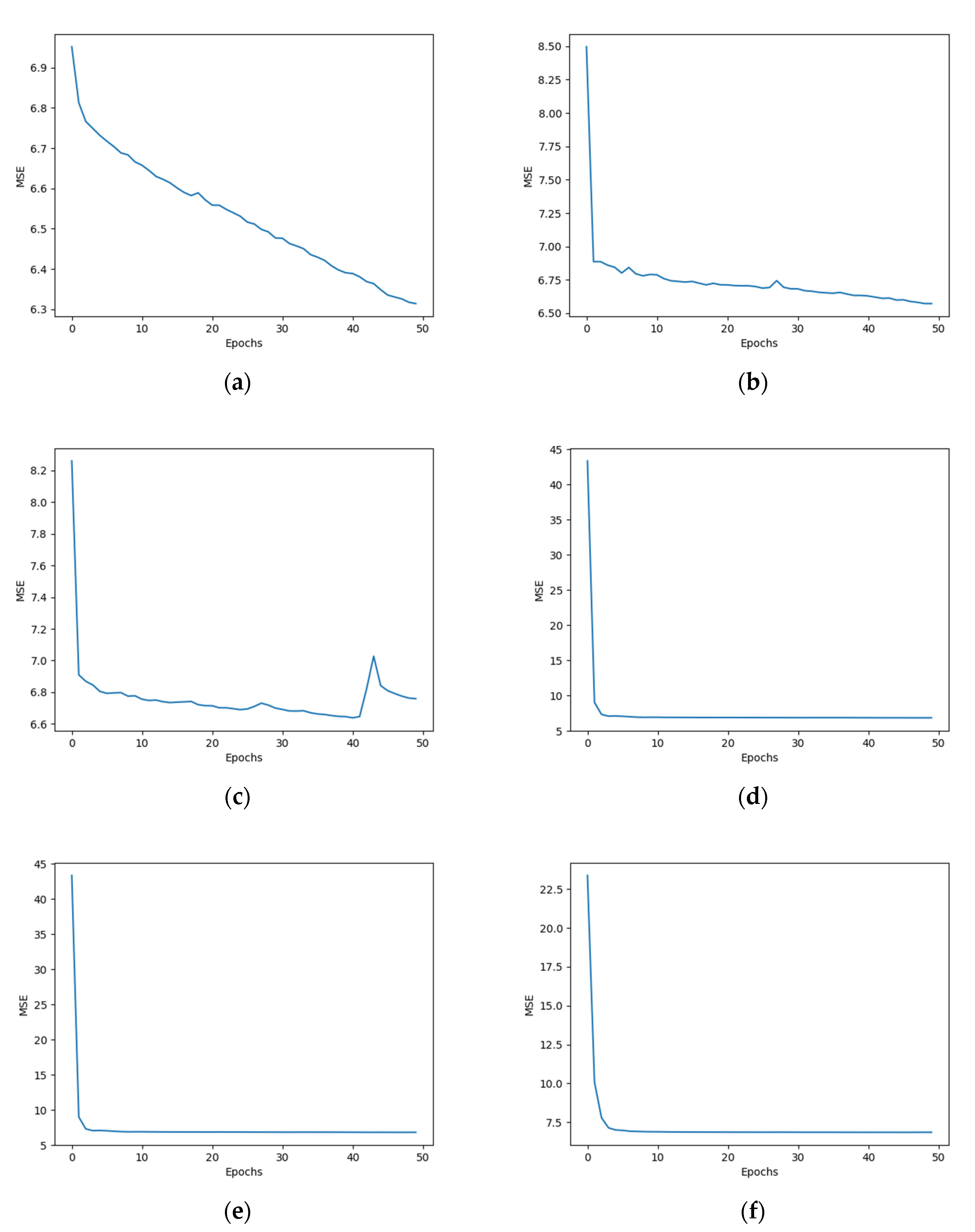
Selection of batchsize and epochs

The data set used in this paper is of a large scale. If we choose to input all the data sets into the network model for training at one time, although this can approach the direction of the extreme value more accurately, the memory requirements are generally relatively high. If only one sample is input into the network model for training at a time, it is found through experiments that the loss function is difficult to converge. Therefore, the experiment in this study did not involve the above two methods to determine the batchsize, but featured an appropriate batchsize through batch gradient descent. We tried different combinations of batchsize and epochs while monitoring the mean square error index of the model and, according to the loss function curve drawn by the mean square error index, the most appropriate curve was selected and the batchsize and epochs corresponding to the curve were taken as the combination of batchsize and epochs used. Since the numbers were stored in the binary form in the computer, the batchsizes we designed were 128, 256, 1024, 2048, 3000, and 4096 (the increase in the batchsize was limited by the GPU memory of the experimental equipment). Epochs were selected to avoid model over-fitting and were set to 50 times based on academic experience. The experimental results are shown in Figure 10.

According to the experimental results in Figure 11, although the loss function curve batchsizes 2048, 3000, and 4096 finally converged when the epoch number was 50, the curve of batchsizes 2048 and 3000 decreased sharply, so the loss function could not be guaranteed to reach the minimum value. As for the curve with a batchsize of 4096, it can be observed that the initial learning rate is relatively large at the beginning, but with the increase in iterations, the learning rate first drops significantly and then slowly, so as to ensure that the loss function can reach the minimum value. Therefore, batchsize was 4096 and epoch number was 50.

(2)

Learning rate

The learning rate represents the network model built in this study with the passage of time and the speed of information accumulation, and choosing the optimal learning rate can determine whether the network model built can converge. If the learning rate is set too high, the model may not converge. If the learning rate is set too low in advance, although it can help the model to converge, it will take a lot of time to make the network model converge to the global minimum. In the field of deep learning, some relatively simple first-order convergence algorithms are commonly used, such as a gradient descent algorithm. The basic formula of gradient descent is shown as follows:

$$w:=w-\alpha \frac{\partial }{\partial w}loss\left(w\right)$$

(20)

where$\alpha$ is the learning rate.

According to the above formula, if the learning rate is relatively low, the loss function of the network will decline very slowly. On the contrary, if the learning rate is set to be high, the range of parameter updates of the network model will become very large, which may lead to the convergence of the network to the local optimal point, or the loss function will suddenly increase.

The learning rate changes constantly in network training. For example, in the initial stage of network model training, the network model parameters are relatively random. According to the prior knowledge of the academic community, a relatively high learning rate was selected to ensure that the loss function decreased faster; after the network model was trained for a period of time, the update characteristics of the parameters could not be greatly updated but were small enough to update.

However, there is no fixed discussion on the initial learning rate. The traditional method is the “trial value method”. This method is relatively inefficient. In the case of a complex network model, this method will consume a lot of calculation time. Therefore, we attempted to use the dragonfly optimization algorithm to find a suitable learning rate for the initial learning rate. The number of dragonflies selected in this experiment was 20, and the number of iterations was 30, The batchsize of the model was selected to be 4096 as determined in the previous experiment, while 50 epochs were selected.

The experimental results of the learning rate are shown in

Table 2. The model’s initial learning rate experiment.

Learning Rate	Coefficient of Determination ${\mathit{R}}^2$	Model Convergence Time ($\mathit{s}$)
0.0459	0.9512	181.0607
0.0999	0.9506	181.1854
0.7318	0.9483	180.4176
0.1635	0.9475	180.9635
0.3529	0.9471	180.7596
0.2938	0.9462	181.8128
0.3121	0.9461	180.3750
0.2916	0.9457	179.7163
0.3736	0.9455	180.3897
0.2337	0.9454	180.8672
0.2821	0.9449	177.7299
0.3230	0.9448	181.1029
0.5124	0.9446	180.4604
0.9005	0.9442	180.7586
0.5064	0.9439	185.3993
0.8575	0.9437	180.5046
0.7217	0.9435	180.8051
0.8892	0.9425	180.3878
0.6537	0.9422	186.0291
0.7850	0.9401	180.4719

.

The model reference index of this experiment is the decision coefficient $R^2$. The closer the value of the decision coefficient $R^2$ is to 1, the better the model prediction accuracy and model fitting effect will be. It can be found from the above table that when the learning rate is 0.0459, the decision coefficient of the model is the highest. To speed up the final convergence speed of the loss function of the model, while ensuring the prediction accuracy, we also aimed to speed up the convergence process of the loss function of the model. Therefore, 0.045913361 was selected as the initial learning rate of the network model.

2.3.2. Data Prediction Experiment of Transformer

In the initial stage of the training network model, the original data set should be segmented into a training set and test set. The test set is an independent data set from the training set. It does not participate in the network model training process like the training set, the purpose is to avoid the over-fitting phenomenon of the prediction model on the test set (model over-fitting means that the model can fit the training set well, but cannot fit the test set well). Therefore, to improve the prediction effect of the model, 80% of the original data set was taken as the training sample of the network model, and the remaining 20% of the original data set was taken as the test set of the network model in the problem of transformer operation data prediction studied here. For the training set, a part of the data was taken as the verification set. The verification set does not participate in the process of model training and is only used to objectively measure the training effect of the model. Cross-validation divides the training data into k groups (k-fold). A verification set was made for these k groups of data, and the remaining k-1 groups of data were used as the training set. Then, the mean squared error of the k group was added and averaged to obtain the cross-verification error. Here, to reflect the difference in prediction indexes before and after network model optimization, the Seq2Seq network model and the Seq2Seq network model optimized by AM were selected for comparison experiments, and k group cross-validation was adopted in the experiment (k = 1 in this experiment). The batchsize and epochs values were 4096 and 50, respectively.

As the experimental results show in

Table 3. Comparison experiment of Seq2Seq and Seq2Seq model based on AM.

Network Model	MAPE	MSE	MAE	RMSE	${\mathit{R}}^2$
Seq2Seq network model	13.55	5300.98	14.01	72.61	0.947
Seq2Seq network model optimized by AM	12.96	4509.45	13.30	68.78	0.951

above, for MAPE indexes, the Seq2Seq network model optimized by AM reduces the error by 0.59% compared with the Seq2Seq network model. For the MSE index, the smaller value of the MSE index indicates that the prediction model is more accurate. It can be found that the Seq2Seq network model optimized by AM is 791.53 lower than the Seq2Seq network model. For the MAE, the Seq2Seq network model optimized by AM is 0.71 lower than the Seq2Seq network model. For the RMSE index, the Seq2Seq network model optimized by AM is 3.83 lower than the Seq2Seq network model. For the $R^2$ index, the closer this value is to 1, the better the prediction performance of the model and the better the fitting of the model. It can be seen that the Seq2Seq network model optimized by AM has a 0.004 improvement in the accuracy of model prediction compared with the Seq2Seq network model. Through the analysis of the above indicators, it is proved that the Seq2Seq network model optimized by AM is superior to the Seq2Seq network model in the prediction performance.

Next, the Seq2Seq network model optimized by AM was used to analyze the fitting errors of 15 label data in detail. Figure 12 shows the predicted results of the 15 tag data.

In Figure 12, the red circles represent the 15 actual ratio rates and the black asterisk represents the predicted values. It can be seen that among the 15 points, most of the predicted values are consistent with the actual values, and only two points, #10 (“5449 line A phase”) and #11 (“5449 line B phase”), have a certain deviation, with the average absolute error being 0.0057% and 0.0014%, respectively.

The complete error of each point is shown in

Table 4. Total error of each point position.

Point Number	Mean Absolute Error of Point Position
main variant I group A phase	0.00027497
main variant I group B phase	0.00002473
main variant I group C phase	0.00011656
main variant II group A phase	0.00000826
main variant II group B phase	0.00000515
main variant II group C phase	0.00004297
main variant III group A phase	0.0000099
main variant III group B phase	0.00007127
main variant III group C phase	0.00000206
5449 Line A phase	0.00569437
5449 Line B phase	0.00138136
5449 Line C phase	0.00008017
5450 Line A phase	0.00001751
5450 Line B phase	0.00029623
5450 Line C phase	0.00004697

. Experimental results show that the prediction error is small.

3. Conclusions

In this paper, an attention mechanism-optimized Seq2seq network is proposed. By introducing the attention mechanism for network optimization, we address the limitations of long-term dependency and the low efficiency of the usage of memory during computation. In the Seq2Seq model construction process, the proposed method effectively achieves long-term dependence without retaining much redundant context information. Through comparative experiments based on the transformer monitoring data set in an electric field, we demonstrate that the proposed method not only greatly improves the training efficiency of the model but also shows good performance in prediction accuracy. Therefore, the proposed method is more versatile and practical in solving electronic transformer error prediction problems.

References

- Joseph, A.; Balachandra, P. Energy Internet, the Future Electricity System: Overview, Concept, Model Structure, and Mechanism. Energies 2020, 13, 4242. [Google Scholar] [CrossRef]
- Li, Z.; Li, H.; Zhang, Z.; Luo, P.; Li, H.; Zhang, W. High-accuracy online calibration system for electronic voltage transformers with digital output. Trans. Inst. Meas. Control. 2014, 36, 734–742. [Google Scholar] [CrossRef]
- Çayci, H. A complex current ratio device for the calibration of current transformer test sets. Metrol. Meas. Syst. 2011, 18, 159–164. [Google Scholar] [CrossRef] [Green Version]
- Xu, Y.; Li, Y.; Xiao, X.; Xu, Z.; Hu, H. Monitoring and analysis of electronic current transformer’s field operating errors. Measurement 2017, 112, 117–124. [Google Scholar] [CrossRef]
- Zhang, Z.; Li, H.; Tang, D.; Hu, C.; Jiao, Y. Monitoring the metering performance of an electronic voltage transformer on-line based on cyber-physics correlation analysis. Meas. Sci. Technol. 2017, 28, 105015. [Google Scholar] [CrossRef] [Green Version]
- Liu, B.; Ye, G.X.; Guo, K.Q.; Mao, A.L.; Wan, G. Calculation method of composite error for electronic current transformers based on Rowgowski coil. High Volt. Eng. 2011, 37, 2391–2397. [Google Scholar]
- Yamada, T.; Kon, S.; Hashimoto, N.; Yamaguchi, T.; Yazawa, K.; Kondo, R.; Kurosawa, K. ECT evaluation by an error measurement system according to IEC 60044-8 and 61850-9-2. IEEE Trans. Power Deliv. 2012, 27, 1377–1384. [Google Scholar] [CrossRef]
- Solovev, D.B.; Gorkavyy, M.A. Current transformers: Transfer functions, frequency response, and static measurement error. In Proceedings of the 2019 International Science and Technology Conference “EastConf”, Vladivostok, Russia, 1–2 March 2019; pp. 1–7. [Google Scholar]
- Lei, T.; Faifer, M.; Ottoboni, R.; Toscani, S. On-line fault detection technique for voltage transformers. Measurement 2017, 108, 193–200. [Google Scholar] [CrossRef]
- Nunes, M.; Gerding, E.; McGroarty, F.; Niranjan, M. The Memory Advantage of Long Short-Term Memory Networks for Bond Yield Forecasting. In Proceedings of the International Conference on Forecasting Financial Markets, Ca’ Foscari University of Venice, Venice, Italy, 19–21 June 2019. [Google Scholar]
- Siami-Namini, S.; Tavakoli, N.; Namin, A.S. A comparative analysis of forecasting financial time series using arima, lstm, and bilstm. arXiv 2019, arXiv:1911.09512. [Google Scholar]
- Jinghang, X.; Wanli, Z.; Shining, L.; Ying, W. Causal Relation Extraction Based on Graph Attention Networks. J. Comput. Res. Dev. 2020, 57, 159–174. [Google Scholar]
- Medeiros, R.P.; Costa, F.B. A wavelet-based transformer differential protection with differential current transformer saturation and cross-country fault detection. IEEE Trans. Power Deliv. 2017, 33, 789–799. [Google Scholar] [CrossRef]
- Ronanki, D.; Williamson, S.S. Evolution of power converter topologies and technical considerations of power electronic transformer-based rolling stock architectures. IEEE Trans. Transp. Electrif. 2017, 4, 211–219. [Google Scholar] [CrossRef]
- Van Der Westhuizen, J.; Lasenby, J. The unreasonable effectiveness of the forget gate. arXiv 2018, arXiv:1804.04849. [Google Scholar]
- Sutskever, I.; Vinyals, O.; Le, Q.V. Sequence to sequence learning with neural networks. arXiv 2014, arXiv:1409.3215. [Google Scholar]
- Cho, K.; Van Merriënboer, B.; Bahdanau, D.; Bengio, Y. On the properties of neural machine translation: Encoder-decoder approaches. arXiv 2014, arXiv:1409.1259. [Google Scholar]
- Przystupa, K. Selected methods for improving power reliability. Przegląd Elektrotech. 2018, 94, 270–273. [Google Scholar] [CrossRef]
- Przystupa, K.; Koziel, J. Analysis of the quality of uninterruptible power supply using a UPS. In 2018 Applications of Electromagnetics in Modern Techniques and Medicine (PTZE); IEEE: Piscataway, NJ, USA, 2018; pp. 191–194. [Google Scholar]
- Tylavsky, D.J.; He, Q.; McCulla, G.A.; Hunt, J.R. Sources of error in substation distribution transformer dynamic thermal modeling. IEEE Trans. Power Deliv. 2000, 15, 178–185. [Google Scholar] [CrossRef]
- Mazurek, P.A.; Michałowska, J.; Koziel, J.; Gad, R.; Wdowiak, A. The intensity of electromagnetic fields in the range of GSM 900, GSM 1800 DECT, UMTS, WLAN in built-up areas. Przeglad Elektrotech. 2018, 94, 202–205. [Google Scholar] [CrossRef] [Green Version]
- Sun, S.; Przystupa, K.; Wei, M.; Yu, H.; Ye, Z.; Kochan, O. Fast bearing fault diagnosis of rolling element using Lévy Moth-Flame optimization algorithm and Naive Bayes. Eksploat. Niezawodn. Maint. Reliab. 2020, 22, 730–740. [Google Scholar] [CrossRef]
- Li, L.L.; Yang, B.; Liang, M.; Zeng, W.; Ren, M.; Segal, S.; Urtasun, R. End-to-end contextual perception and prediction with interaction transformer. arXiv 2020, arXiv:2008.05927. [Google Scholar]
- Wu, P.; Lu, Z.; Zhou, Q.; Lei, Z.; Li, X.; Qiu, M.; Hung, P.C. Bigdata logs analysis based on seq2seq networks for cognitive Internet of Things. Future Gener. Comput. Syst. 2019, 90, 477–488. [Google Scholar] [CrossRef]
- Wang, J.; Kochan, O.; Przystupa, K.; Su, J. Information-measuring system to study the thermocouple with controlled temperature field. Meas. Sci. Rev. 2019, 19, 161–169. [Google Scholar] [CrossRef] [Green Version]
- Chung, J.; Gulcehre, C.; Cho, K.; Bengio, Y. Empirical evaluation of gated recurrent neural networks on sequence modeling. arXiv 2014, arXiv:1412.3555. [Google Scholar]
- Graves, A.; Fernández, S.; Schmidhuber, J. Bidirectional LSTM networks for improved phoneme classification and recognition. In Proceedings of the International Conference on Artificial Neural Networks 2005, Warsaw, Poland, 11–15 September 2005; pp. 799–804. [Google Scholar]
- Jun, S.; Przystupa, K.; Beshley, M.; Kochan, O.; Beshley, H.; Klymash, M.; Wang, J.; Pieniak, D. A Cost-Efficient Software Based Router and Traffic Generator for Simulation and Testing of IP Network. Electronics 2019, 9, 40. [Google Scholar] [CrossRef] [Green Version]
- Liu, J.; Fan, X.; Zhang, Y.; Zhang, C.; Wang, Z. Aging evaluation and moisture prediction of oil-immersed cellulose insulation in field transformer using frequency domain spectroscopy and aging kinetics model. Cellulose 2020, 27, 7175–7189. [Google Scholar] [CrossRef]
- Kozieł, J.; Przystupa, K. Using the FTA method to analyze the quality of an uninterruptible power supply unitreparation UPS. Przeglad Elektrotech. 2019, 95, 37–40. [Google Scholar] [CrossRef] [Green Version]
- Przystupa, K. An attempt to use FMEA method for an approximate reliability assessment of machinery. In Proceedings of the ITM Web of Conferences, Lublin, Poland, 23–25 November 2017; EDP Sciences: Paris, France, 2017; Volume 15, p. 5001. [Google Scholar]
- Fang, M.T.; Chen, Z.J.; Przystupa, K.; Li, T.; Majka, M.; Kochan, O. Examination of Abnormal Behavior Detection Based on Improved YOLOv3. Electronics 2021, 10, 197. [Google Scholar] [CrossRef]
- Zhang, Y.; Yu, M.; Li, N.; Yu, C.; Cui, J.; Yu, D. Seq2seq attentional siamese neural networks for text-dependent speaker verification. In Proceedings of the ICASSP 2019–2019 IEEE International Conference on Acoustics, Speech and Signal Processing (ICASSP), New Orleans, CA, USA, 5–9 March 2017; pp. 6131–6135. [Google Scholar]