Research on Online Diagnosis Method of Fuel Cell Centrifugal Air Compressor Surge Fault

Abstract

Stable operation of fuel cell air compressions is constrained by rotating surge in low flowrate conditions. In this paper, a diagnosis criterion based on wavelet transform to solve the surge fault is proposed. First of all, the Fourier transform was used to analyze the spectral characteristics of the outlet flowrate. Before wavelet transform was used, the data are standardized. This step eliminated the influence of the flowrate’s absolute value. Then, the wavelet coefficients under characteristic frequencies were extracted. Finally, the diagnosis criterion’s threshold, which indicates the surge occurrence, was defined from the perspective of safety margin. The criterion threshold alerted a surge only 1 s after it occurred. The analysis results show that the criterion meets with the expectation, and it can be used for the control of anti-surge valve.

1. Introduction

Stringent environmental reforms and enforced low carbon footprint stimulated interest towards emission-free green power generation. Factors such as high efficiency, low noise, good dynamic response and low aggression to environment elevated the research focus on proton exchange membrane (PEM) fuel cell in recent years [1,2]. Furthermore, almost all automobile manufacturers in the world have paid great attention to mastering PEM fuel cell technology [3].

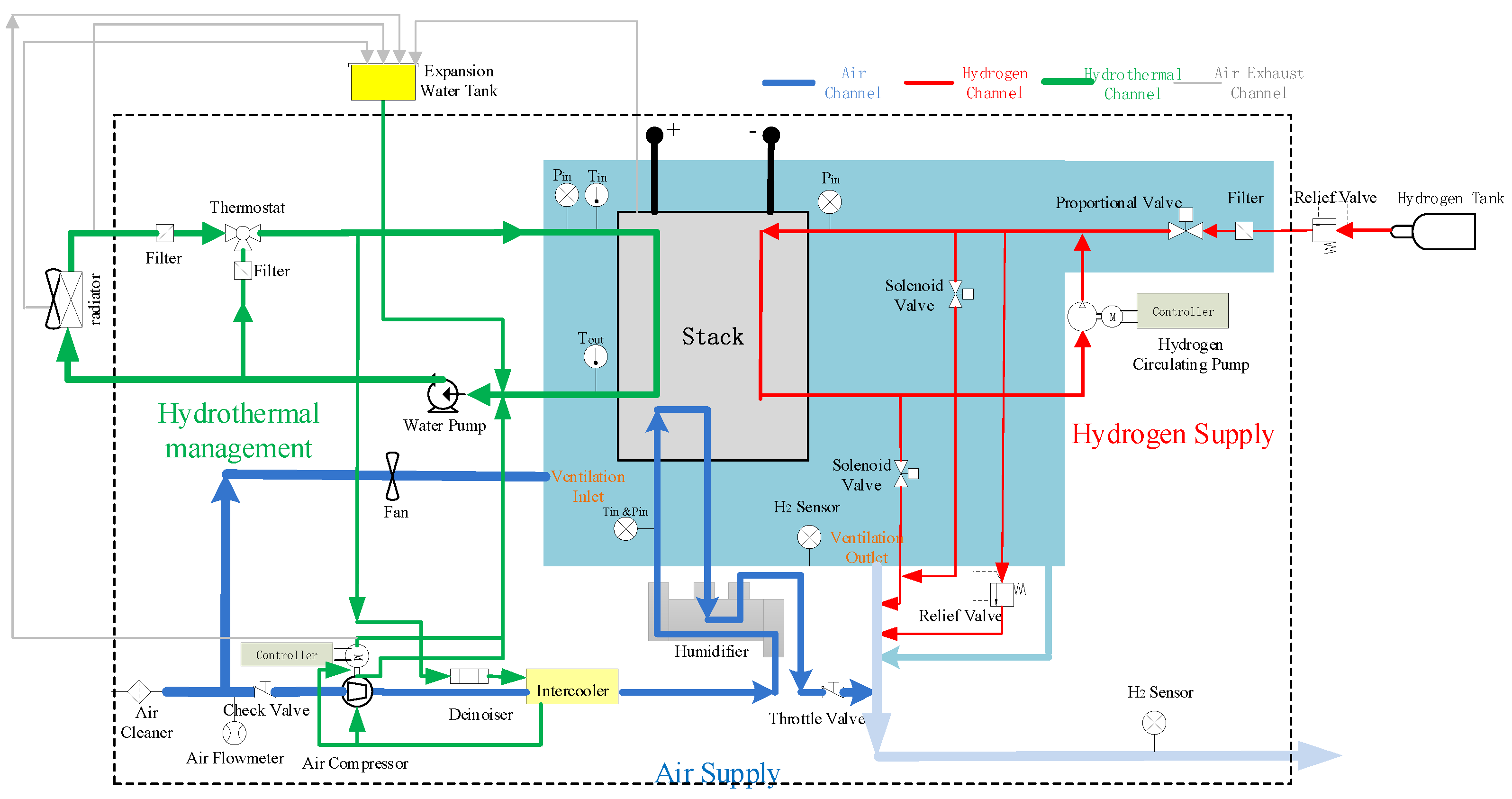
PEM fuel cell is a device that generates electricity through the electrochemical reaction of hydrogen and oxygen [4,5]. It can be divided into the following four subsystems, including the stack system, the air supply subsystem, the hydrogen supply subsystem, and the hydrothermal management subsystem, as shown in Figure 1. The air supply subsystem provides air with appropriate flow and pressure for the electrochemical reaction, and its function mainly depends on compressing air by compressor. When the air supply system is not enough to support the normal electrochemical reaction, the fuel cell system will have a gas starvation failure, which will affect the performance output of the fuel cell stack [6,7]. The air compressor is a key component for supercharging in the fuel cell air supply system, and it is also the most energy-consuming component. Generally speaking, about 20% of the power generated by the fuel cell system is used to drive the air compressor [8]. Therefore, choosing a suitable air compressor has a vital impact on improving the overall performance of the fuel cell system.

To date, there are two main types of air compressors often used in fuel cell systems, screw air compressors and centrifugal air compressors [9]. Among them, centrifugal air compressors have become more attractive in recent years due to their simplicity, compactness, higher efficiency, and lower prices [10,11,12].

However, centrifugal air compressors may cause damaging surge under small flow conditions [13,14,15,16]. During the operation, when the inlet flow rate is reduced to a certain value, the gas will not be able to adhere to the rotating impeller, resulting in the phenomenon of rotating separation. After separating, the pressure in air compressor cavity will drop because the gas cannot be pushed by the impeller. At this time, the higher pressure gas at the outlet side will flow back into the cavity due to the pressure difference. When the flow of the air compressor is replenished, the impeller can restore the ability to do work on the gas and discharge the inverted air flow again. If the gas flow supply at the inlet cannot keep up, it will cause the pressure in the cavity to continue to drop, and repeat the above abnormal process. This phenomenon is the surge of the centrifugal air compressor.

The surge failure will have an adverse effect on the air compressor itself. For example, due to strong pulsation and periodic oscillation, the impeller vibrates strongly, which greatly increases the stress of the impeller and increases the noise. In severe cases, bearings and seals may be damaged, which can cause serious accidents. In addition, surge will also cause the fuel cell air subsystem to supply instability, resulting in the gas starvation and a decrease in output performance of fuel cell system. Considering that in common vehicle driving cycles, idling and low-speed scenes occupy a large proportion, the fuel cell output power is small, and the required air flow rate is relatively low. At this time, this kind of small flow condition is easy to cause surge failure of the centrifugal air compressor.

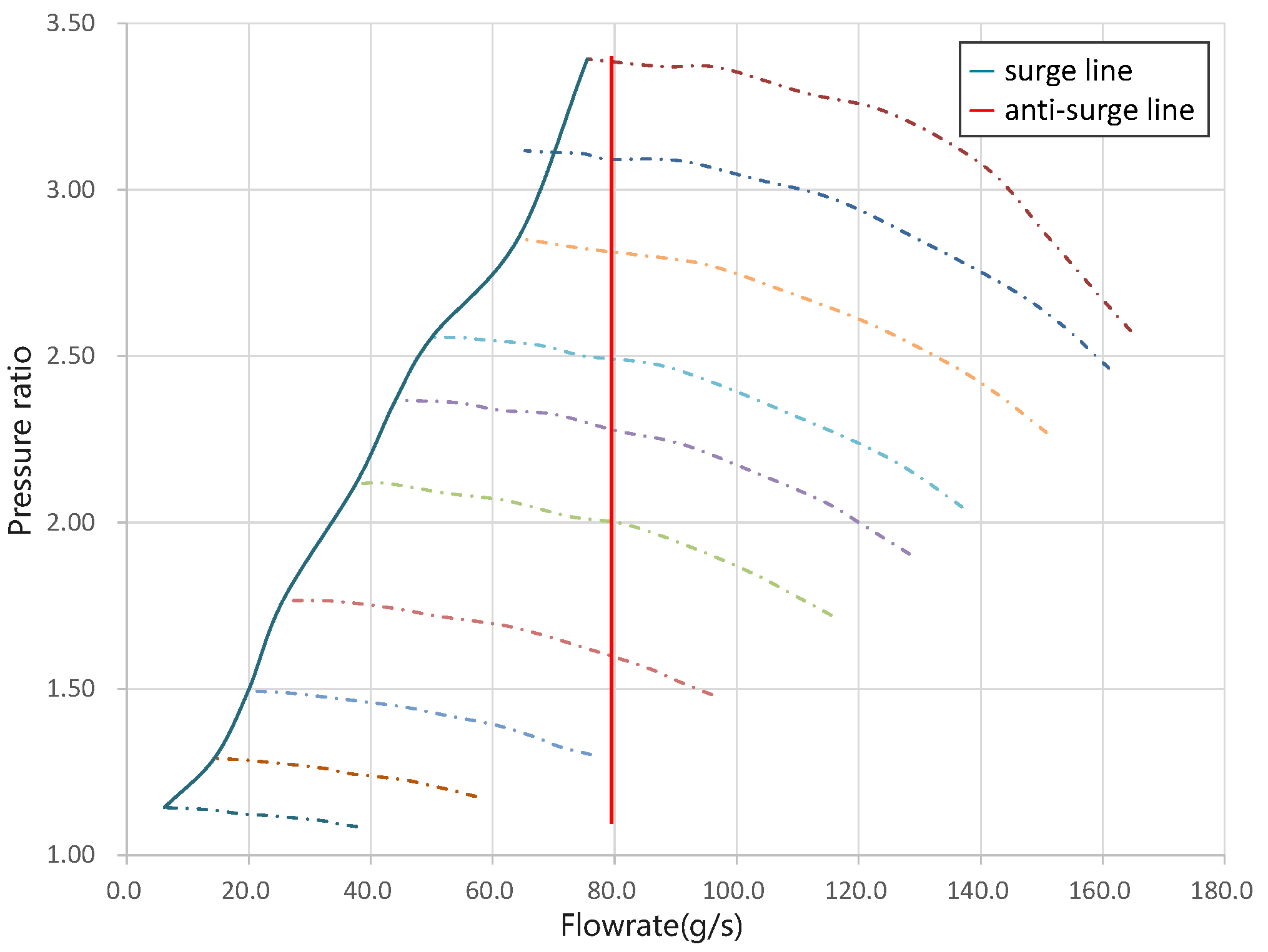
Therefore, the centrifugal air compressor must be diagnosed in real time, especially when the surge trend occurs during its operation, corresponding measures should be taken to prevent the occurrence of surge in time based on the real-time diagnosis result. At present, the widely used anti-surge methods in engineering can be divided into two types, the fixed limit flow method and the variable limit flow method. The former mainly fixes a single limit flow rate [17,18,19], as shown in Figure 2, regardless of the air compressor speed and pressure ratio, when the actual flow rate is less than this limit flow value, the bypass valve located at the outlet of the centrifugal air compressor is opened. This method is suitable for centrifugal air compressors with little range of speed, because a large change in speed means a large change in flow, and the flow limit is generally set to a higher value. When the speed of the centrifugal air compressor is adjusted as needed to reduce the flow rate to below the flow limit value, the anti-surge valve is opened according to the control strategy and, at this time, part of the air is discharged through the bypass valve, which causes a waste of energy in the centrifugal air compressor. The second variable limit flow method overcomes the shortcomings of the former’s low efficiency. According to the surge line provided by the supplier, an anti-surge line containing a variable limit flow (also called a variable limit flow line) is set up [20,21], as shown in Figure 3. Once the operating point of the centrifugal air compressor touches the anti-surge line, it is considered that there is a trend of surge occurrence. Based on this variable limit flow line, the controller can determine the opening and closing of the bypass valve according to the measured flow rate and pressure ratio and the position relationship of the limit flow line on the map, thereby preventing the occurrence of surge.

The initial anti-surge line is derived from the surge data obtained by the air compressor manufacturer under specific experimental conditions. However, due to factors such as different system pipelines, different operating environments, or aging of the centrifugal air compressor during engineering applications, the anti-surge line drift will occur. Therefore, in reality, it is usually necessary to measure the state of the air medium in real time through multiple pressure, flow and temperature sensors to correct the anti-surge line. At present, the surge point detect methods of centrifugal air compressors mainly focus on four methods, which are experimental detection method [22,23], signal processing detection method, nonlinear modeling method [24], and artificial intelligence method [25,26]. Li et al. [27] propose signal processing and pattern recognition methods to extract the characteristic information from the vibration or sound signal of the centrifugal air compressor, and train a certain neural network offline to identify the surge state or the trend of surge occurrence. However, after running for a period of time, factors such as changes in pipeline flow resistance and aging of mechanical parts can also cause the pulse spectrum and surge line of the centrifugal air compressor to drift, and the neural network model trained off-line will misjudge. In addition, the characteristic information extraction of vibration or sound signals requires an additional set of acceleration or sound wave sensors, which increases the cost and complexity of the system.

After the working point of the centrifugal air compressor approaches or enters the surge zone, the air is continuously pressed out of the cavity and then refilled, and the air outlet flow and pressure fluctuate sharply [14,28]. The object of this paper is to extract characteristic information from the outlet flow rate of the centrifugal air compressor by using signal analysis methods without adding additional sensors, so as to realize the purpose of real-time monitoring of the surge trend of the centrifugal air compressor, and provide a basis for the anti-surge strategy.

When the centrifugal air compressor surges, the flowrate will fluctuate, and the frequency is obviously different from that under normal conditions. Based on this feature, this paper proposes the following framework to predict the trend of surge.

①

The fast Fourier transform is performed on the flow signal under normal conditions and surge conditions, respectively, so as to put forward the hypothesis that the characteristic frequency of the centrifugal air compressor flowrate during surge is different from the normal time.

②

Based on the above assumption, the flow rate is further analyzed by complex morlet wavelet transform to perform time-frequency analysis to verify that the real-time signal processing method can find out the tendency to surge.

③

The same analysis on the flow signals at different speeds is done to mutually verify the accuracy of our proposed methods.

2. Theoretical Background

Fourier transform is the most widely used time–frequency conversion method, which can convert time-domain signals into frequency-domain signals. However, the traditional Fourier transform is only suitable for deterministic stationary signals. The value of the frequency domain signal $F\left(\omega \right)$ at any frequency $\omega$ is determined by the value of $f\left(t\right)$ in the entire time domain, which means that the information of the signal $f\left(t\right)$ in the entire time domain must be obtained to get the full frequency $F\left(\omega \right)$ of the domain. In order to overcome the shortcomings of this global analysis, researchers introduce the window function $g\left(t\right)$, and use it to perform convolution operation with the original signal to reflect the local characteristics of the original signal $f\left(t\right)$. This method is called short-time Fourier transform (STFT), and its mathematical is described in Equation (1).

$$F(t,\omega )={\int }_{-\infty }^{+\infty }\left[f\left(\tau \right)g(\tau -t)\right]e^{-j\omega \tau }d\tau$$

(1)

After this transformation, the frequency domain function $F(t,\omega )$ corresponding to different time t can be obtained. However, according to the uncertainty principle, no matter what type of window function is used, the STFT can not meet the accuracy requirements in the two dimensions of time and frequency at the same time because the product of its corresponding time uncertainty ${\delta }_t$ and frequency uncertainty ${\delta }_{\omega }$ is not less than a fixed value. In addition, STFT selects a fixed window, and the window width will not change during one STFT transformation, and the corresponding time resolution and frequency resolution are also fixed, and cannot be dynamically adjusted with the frequency of non-stationary signals. This means that when analyzing a section of non-stationary signal, how to choose an appropriate window width becomes very difficult. Therefore, STFT cannot meet the needs of non-stationary signal analysis [29,30].

The wavelet transform uses the wavelet whose amplitude gradually decays and the original data $f\left(t\right)$ to perform convolution calculation as shown in Equation (2).

$$F(a,b)=\frac{1}{\sqrt{a}}{\int }_{-\infty }^{\infty }f\left(t\right)\mathsf{\Psi }\left(\frac{\tau -b}{a}\right)dt$$

(2)

The type of wavelet transform depends on the type of wavelet basis function $\mathsf{\Psi }(·)$ used. According to continuity, wavelet transform can be divided into continuous wavelet transform and discrete wavelet transform, and the former is more suitable for signal feature extraction [31]. Orthogonal wavelet function is generally used as the wavelet basis function of discrete wavelet transform, and can also be used for continuous wavelet transform [32], while non-orthogonal wavelet functions are usually used for continuous wavelet transformation. In addition, selecting non-orthogonal complex wavelet functions can obtain the amplitude and phase characteristic information of the time domain signal in the frequency domain. When choosing the wavelet basis function, considering the vibration signal caused by the failure of common fluid machinery, it usually has the characteristics of impact attenuation [33,34], and the Morlet wavelet is a cosine signal with exponential attenuation on both the left and right sides. Therefore, when performing continuous wavelet transform on the output flow signal of the centrifugal air compressor, we think it is appropriate to select the non-orthogonal complex Morlet function as the wavelet basis function, and the corresponding wavelet transformation is called cmor wavelet transform for simplicity.

The wavelet basis function used in cmor wavelet transform is described in Equation (3).

$$\mathsf{\Psi }\left(t_{\mathrm{m}}\right)=\frac{1}{\sqrt{\pi f_{\mathrm{b}}}}exp\left(\frac{-t_{\mathrm{m}}^2}{f_{\mathrm{b}}}\right)exp\left(j2\pi f_{\mathrm{c}}{t}_{\mathrm{m}}\right)$$

(3)

In Equation (3), the wavelet function is obtained by multiplying a Gaussian function and a trigonometric function, where $f_{\mathrm{b}}$ is the bandwidth parameter and $f_{\mathrm{c}}$ is the center frequency. The relationship between the parameter $t_{\mathrm{m}}$ and the real time t is shown in Equation (4).

$$t_{\mathrm{m}}=\frac{\tau -b}{a}$$

(4)

2.1. Scale and Shift

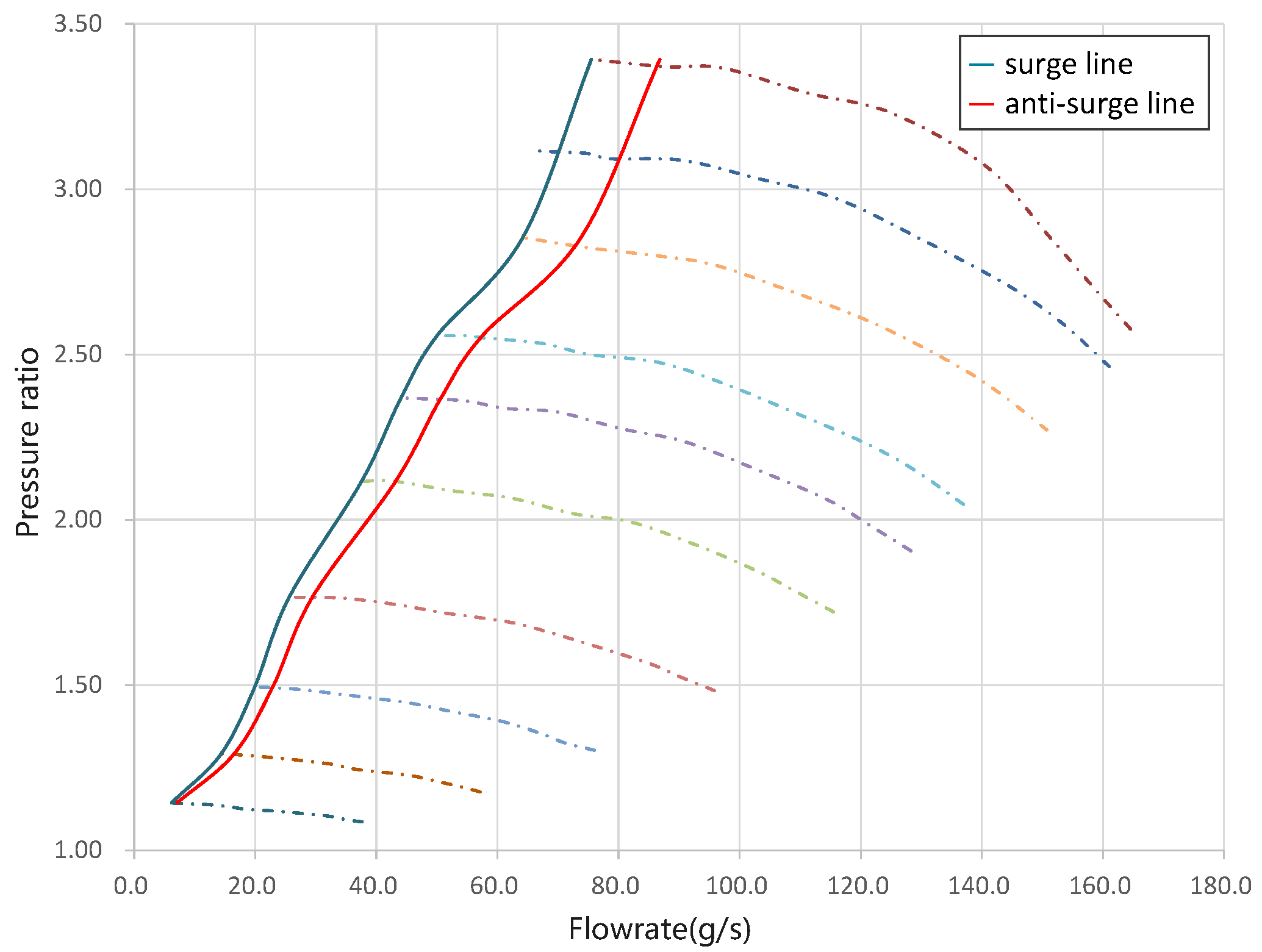
In Equation (4), a and b respectively represent the scale parameter and the shift parameter, and they determine the range and position of the wavelet function. As showed in Figure 4a, the value of a is related to the expansion and contraction of the wavelet function. When a increases, the wavelet function is elongated, and when a decreases, the wavelet function shrinks. Therefore, the relationship among the real frequency f of the signal, the center frequency $f_{\mathrm{c}}$ and the sacle parameter a is shown in Equation (5). As showed in Figure 4b, the value of b is related to the position of the wavelet function on the time axis. When b increases, the wavelet function shifts positively on the time axis, and vice versa. It is worth mentioning that the value of b is exactly the center time of wavelet function.

$$f=\frac{f_{\mathrm{c}}}{a}$$

(5)

2.2. Bandwidth and Center Frequency

As mentioned earlier, the wavelet function is obtained by multiplying a trigonometric function $h\left(t_{\mathrm{m}}\right)$ and a Gaussian function $g\left(t_{\mathrm{m}}\right)$. In the Equation (6), the parameter $f_{\mathrm{c}}$ is related to the period of the trigonometric function, here we call it the center frequency of the wavelet function, and the ratio of it to the real frequency is equal to a, that is, the frequency of the analyzed signal can be determined by setting the value of a and $f_{\mathrm{c}}$. In the Equation (7), the parameter $f_{\mathrm{b}}$ determines the size of the Gaussian window because it corresponds to the variance of the Gaussian function and the relationship can be expressed in Equation (8).

$$g\left(t_{\mathrm{m}}\right)=\frac{1}{\sqrt{\pi f_{\mathrm{b}}}}exp(-\frac{t_{\mathrm{m}}^2}{f_{\mathrm{b}}})$$

(6)

$$h\left(t_{\mathrm{m}}\right)=exp\left(j2\pi f_{\mathrm{c}}{t}_{\mathrm{m}}\right)$$

(7)

$$f_{\mathrm{b}}={\sigma }^2$$

(8)

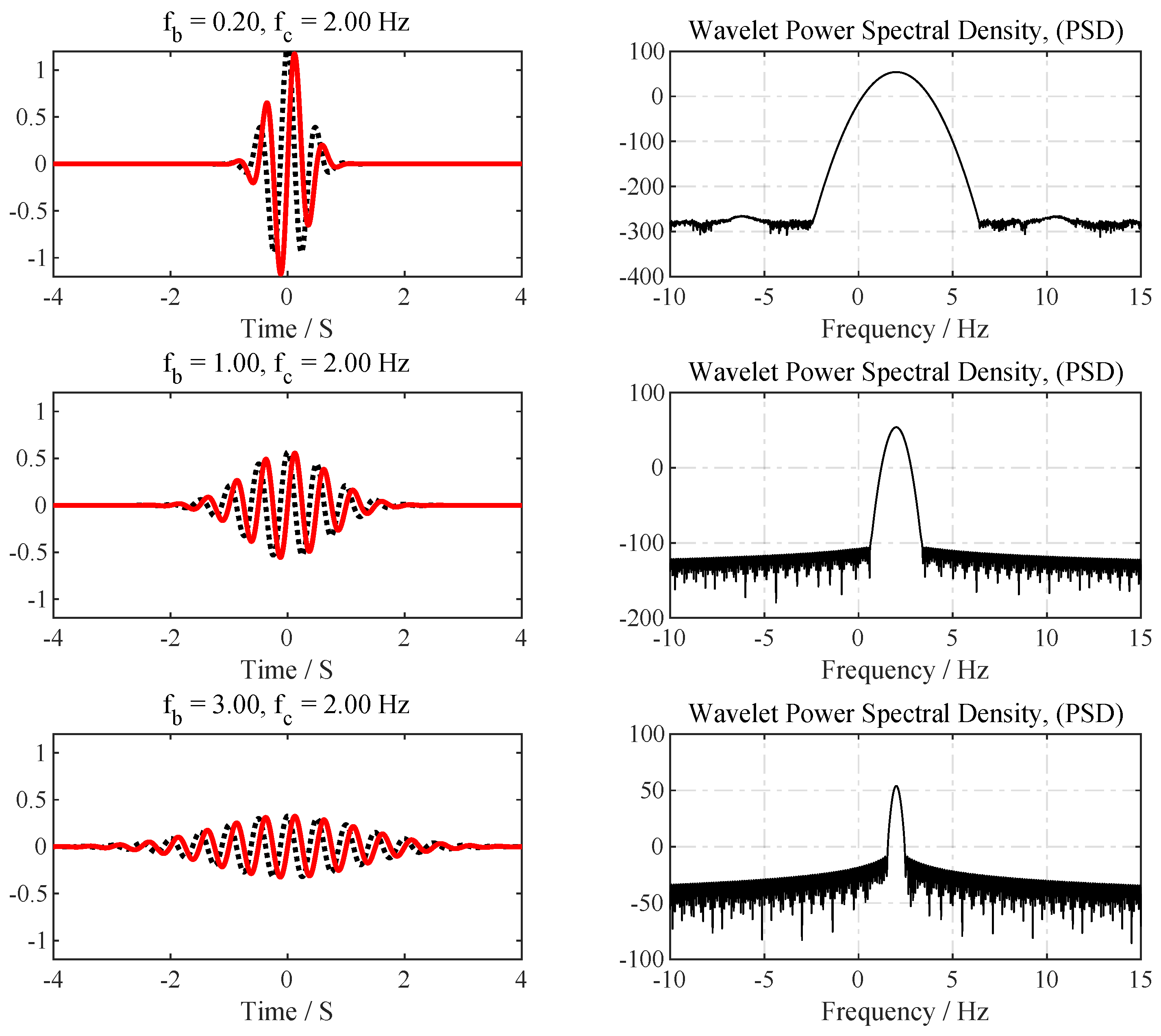
According to the characteristics of the Gaussian function, the larger the variance, the wider the Gaussian window, so the parameter $f_{\mathrm{b}}$ can determine the time resolution and frequency resolution of the wavelet function. In order to show the influence of $f_{\mathrm{b}}$ more intuitively, the center frequency $f_{\mathrm{c}}$ is fixed at 2 Hz, and $f_{\mathrm{b}}$ is set to 0.2 Hz, 1 Hz, 3 Hz respectively, and the corresponding wavelet functions and their power spectral density (PSD) are shown in Figure 5. It can be seen from the figure that when $f_{\mathrm{b}}$ increases, the width of the wave in the time domain as well as the number of cycles of the sinusoidal wave increases, and the temporal resolution decreases.

The choice of $f_{\mathrm{b}}$ and $f_{\mathrm{c}}$ in Complex Morlet wavelet basis function is an optimization problem, and the different combinations of the two parameters have a great influence on the analysis results. In this paper, we take Shannon entropy $E_{\mathrm{n}}$ [33,35], as shown in Equation (9), as the objective optimization function, where M is the number of wavelet coefficients, and $C_{\mathrm{j}}$ is the wavelet coefficient. By solving the optimization problem shown in Equation (10), the optimal value of the bandwidth $f_{\mathrm{b}}$ and the center frequency $f_{\mathrm{c}}$ can be 3 Hz.

$$E_{\mathrm{n}}=-\sum _{\mathrm{i}=1}^M{d}_{\mathrm{i}}log{d}_{\mathrm{i}},d_{\mathrm{i}}=\frac{C_{\mathrm{i}}}{{\sum }_{\mathrm{j}=1}^M{C}_{\mathrm{j}}}$$

(9)

$$\underset{\left(f_{\mathrm{b}}^{*},f_{\mathrm{c}}^{*}\right)}{min}\left\{E_{\mathrm{n}}\right\}$$

(10)

The cmor wavelet transform has the powerful advantages of time-frequency analysis [36]. Under a certain scaling scale $a_{\mathrm{i}}$, the wavelet basis function is convolved with the time domain signal $f\left(t\right)$. When the characteristic frequency of a piece of data near the translation factor $b_{\mathrm{i}}$ is the same or close to the frequency of the wavelet basis function, the convolution value is abnormally large. This fact actually conveys two pieces of information, first is that the characteristic frequency of a certain segment of the time-domain signal is the same as the wavelet basis function, and the second is that the same characteristic frequency occurs at the moment corresponding to the translation factor $b_{\mathrm{i}}$.

3. Experiment Introduction and Data Pre-Analysis

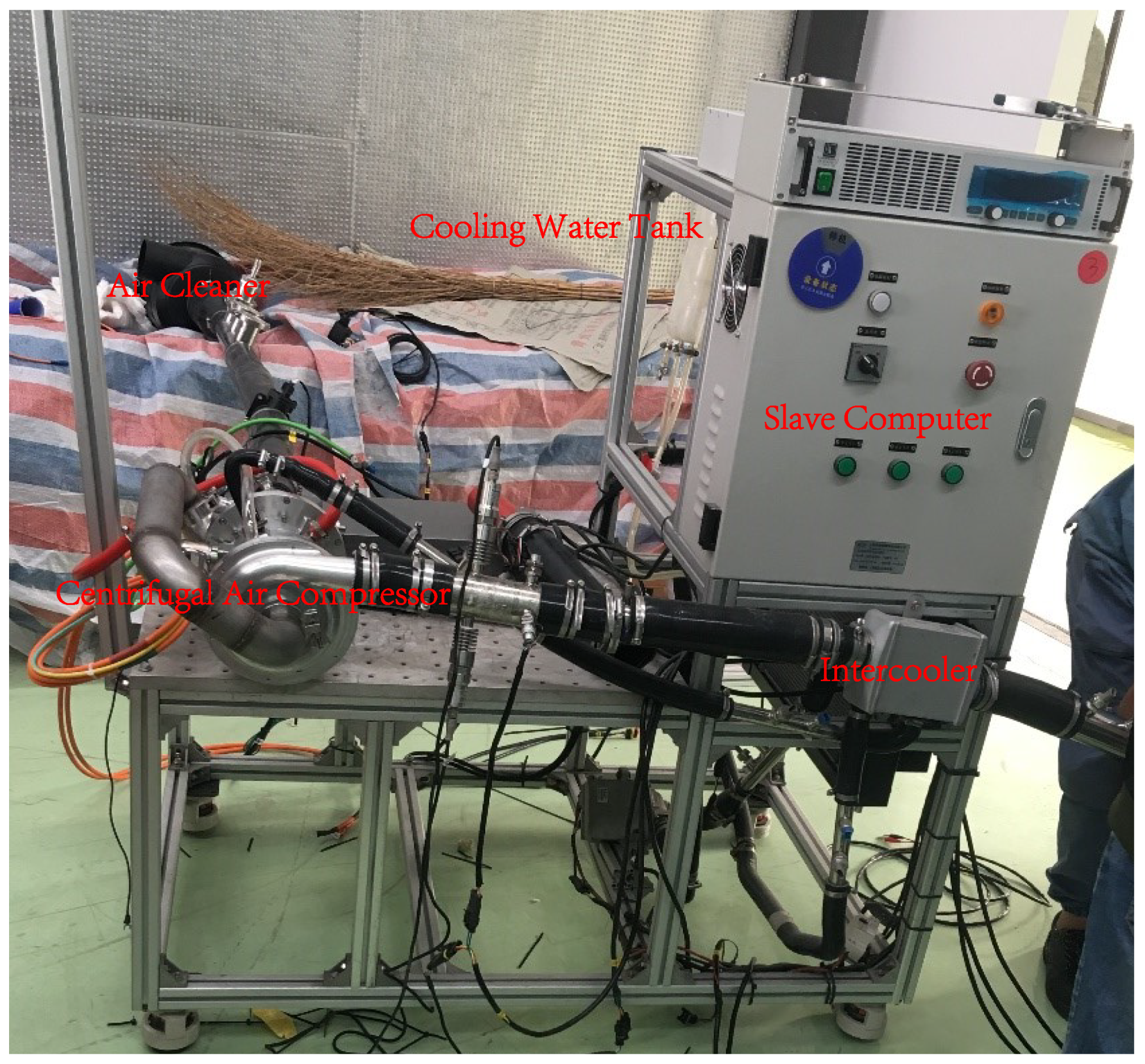
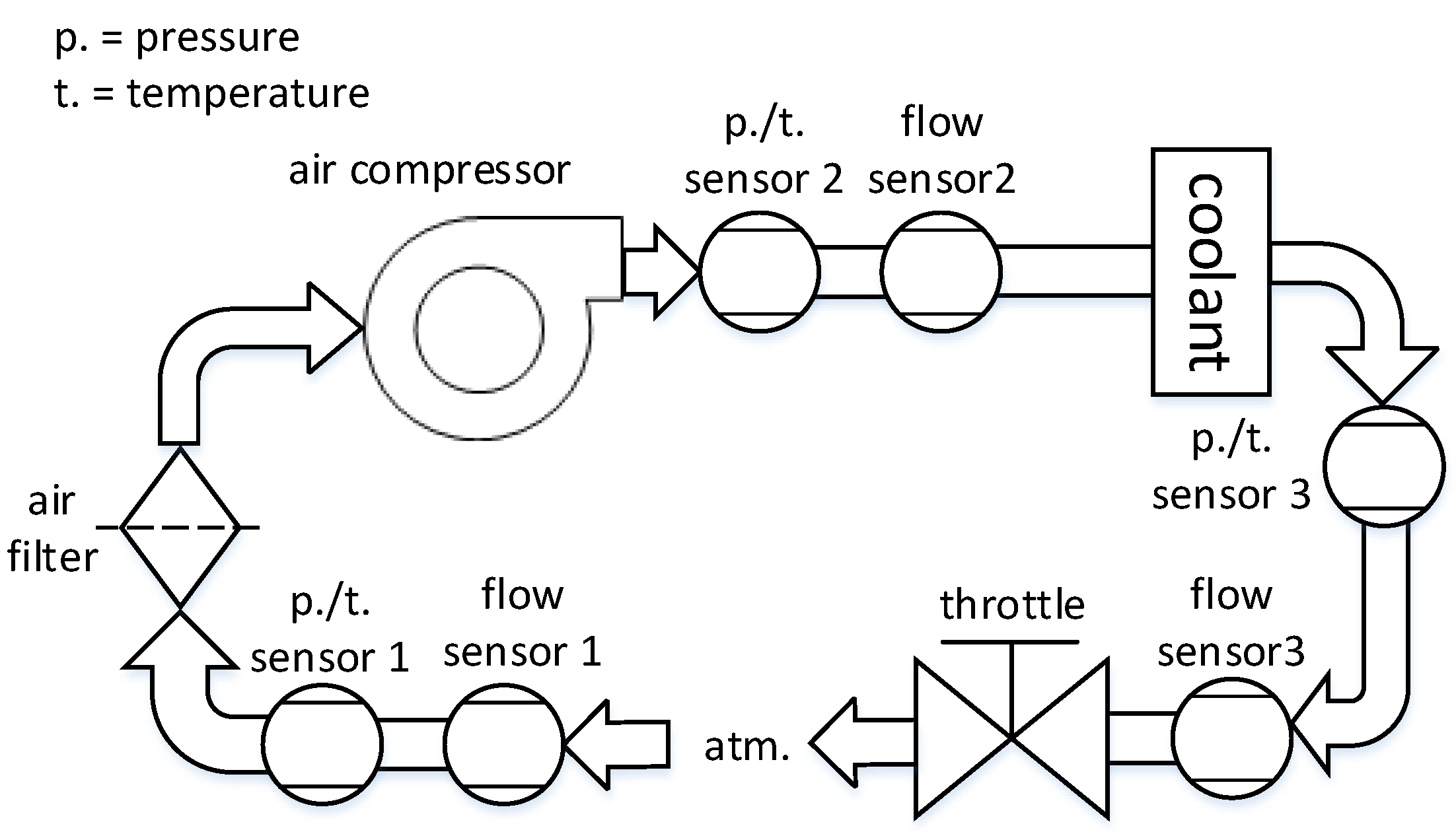
In order to obtain the outlet flow data of the centrifugal air compressor, the air compressor test bench as shown in Figure 6 was built, which can be used for performance testing and map verification of various types of centrifugal air compressors. In this paper, the maximum flow rate of the centrifugal air compressor we tested is about 170 g/s, the maximum pressure ratio is about 3.3, and the maximum speed is 94,000 rpm. The structure and principle of this test bench can be simplified as shown in Figure 7.

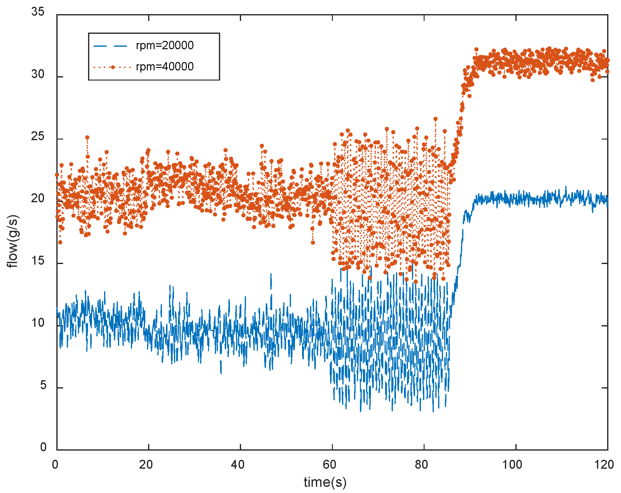
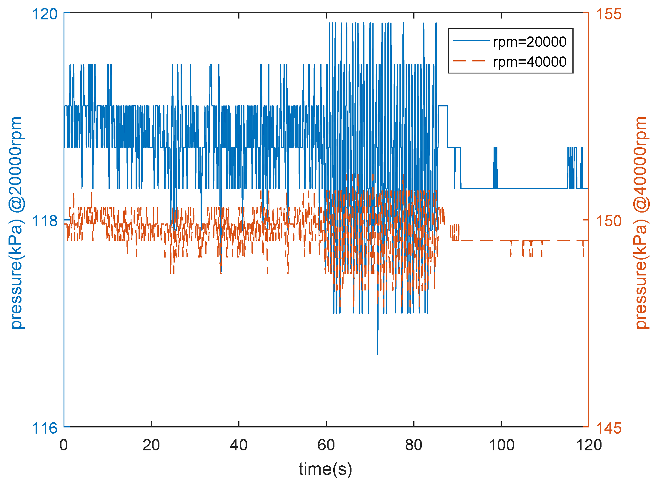
First, we make the centrifugal air compressor work under the two speed conditions of 20,000 rpm and 40,000 rpm, respectively, and slowly increase the pressure ratio by adjusting the throttle opening, so that the operating point of the air compressor is close to surge. Figure 8 and Figure 9 show the flow data and pressure data, respectively, recorded at the outlet of the air compressor through the data acquisition equipment.

In the data recorded in Figure 8, the centrifugal air compressor works close to surge from 0 to 60 s and has shown a tendency to surge, which is reffered to as the quasi-surge zone. In this area, we think it has the danger of surge but not surge exactly, and judging by the principle of the above variable limit flow method, the anti-surge valve should be opened at this time. During 60 s to 85 s, the centrifugal air compressor enters the surge zone, and the abnormally large flow fluctuations may cause irreversible damage to the centrifugal air compressor, which is a working condition that should be avoided in advance. At 85 s, surge is observed and the throttle opening is adjusted to reduce the pressure ratio, which can drag the operating point of air compressor from surge zone to allowable operation zone.

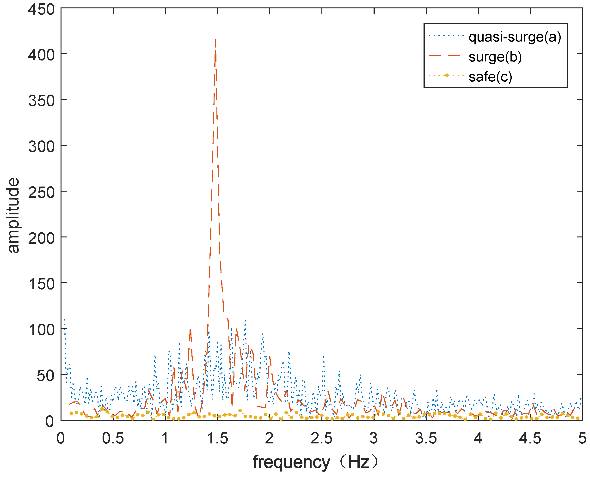
From an intuitive point of view, the amplitude of the flow rate change in the quasi-surge zone and the surge zone is obviously much larger than that in the allowable operation area, which is two to four times that of the allowable operation area. At the same time, the flow value data in the quasi-surge zone and the surge zone show a certain low-frequency fluctuation as a whole. For the sake of clarity and length, the following uses the data at 20,000 rpm as an example to perform Fourier transform analysis. In order to verify the above conjecture and detect its dominant frequency, Fourier transform [12] was performed on the data of the above three regions, and the results are shown in Figure 10.

In Figure 10, the energy distribution in the Fourier transform result of curve c, which represents the safe zone, is relatively scattered, and the fluctuation of the flow in this zone can almost be regarded as white noise. Besides, the energy in curve a and curve b, which represent quasi-surge zone and surge zone, respectively, are relatively concentrated, and the main frequencies of the two are very close, around 1.4 Hz. At the same time, it can be clearly seen that the dominant frequency of the surge zone is more obvious than that of the quasi-surge zone, and the energy is very concentrated and prominent at 1.4 Hz in the surge zone. This result shows that surge has a unique characteristic frequency, and it exists in both the quasi-surge zone and the surge zone.

4. Time–Frequency Feature Extraction of Signals

4.1. Analysis of Wavelet Transform

According to the complex Morlet wavelet transform theory and its application method introduced in Section 1, the continuous complex Morlet wavelet transform is performed on the outlet flow signal of the centrifugal air compressor. In order to mutually verify the characteristic frequency determined by the above Fourier transform result, the sweep frequency range of the wavelet transform is set to 0–10 Hz [37].

A time unit of 4 s is used to intercept and collect the flow signal and transmit it to the wavelet transform algorithm as a signal stream. The data of less than 4 s is filled with the data at the first and last moments. The absolute value of the flow is different at different speeds, which will inevitably affect the amplitude of the wavelet coefficients obtained by the wavelet transform, which makes it impossible to formulate a suitable anti-surge strategy. A 0–1 normalization of original data is firstly done before the wavelet transform.

$$q_{\mathrm{norm}}=\frac{q-q_{min}}{q_{max}-q_{min}}$$

(11)

where q is the original flow data, $q_{min}$ and $q_{max}$ are the minimum and maximum values of the data per unit time, respectively.

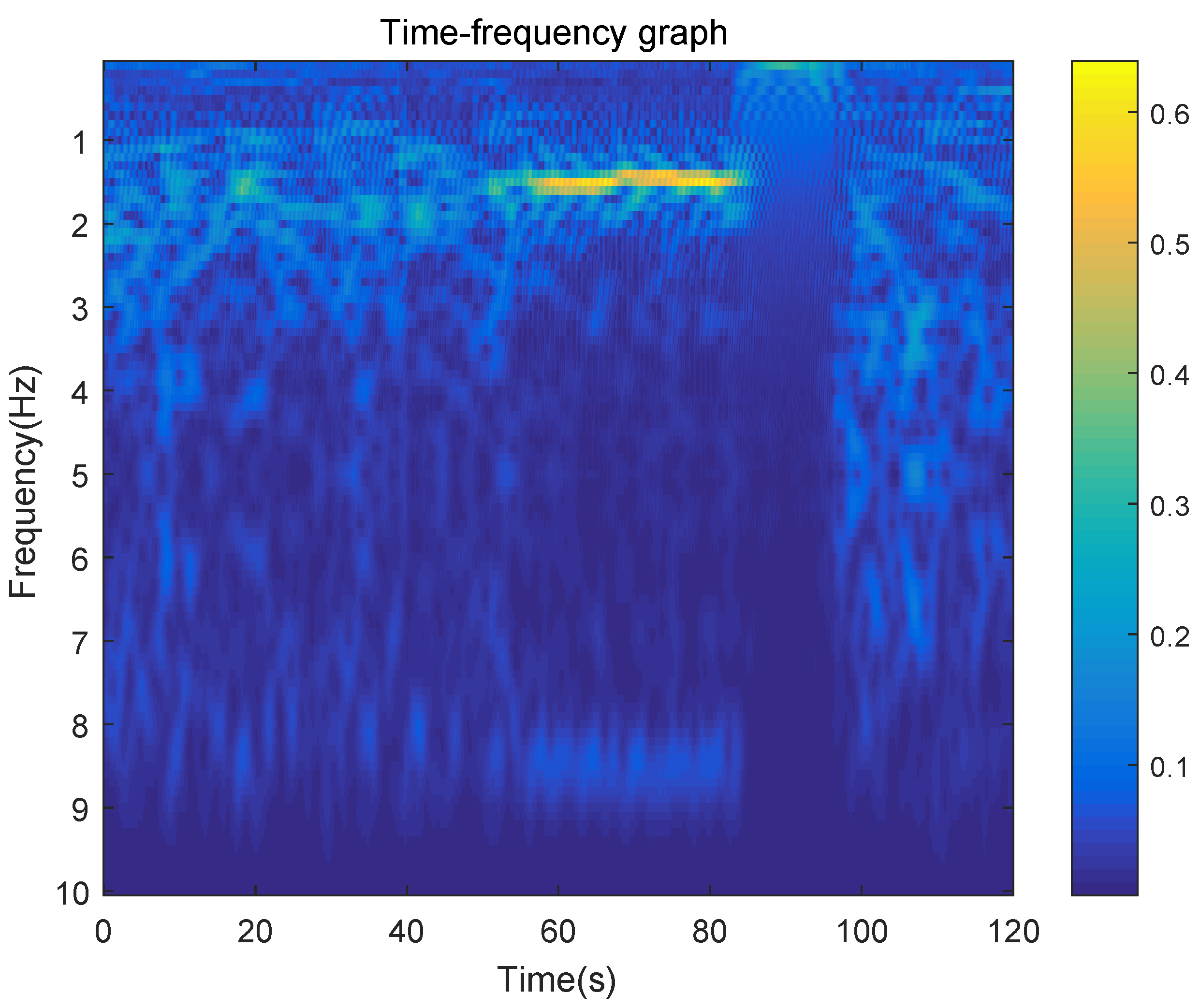
The data from the 1.5 s to 0.5 s from the bottom of the wavelet transform result per unit time is averaged as the result of the time period. With the sampling time of 0.1 s as the step length, repeat the above steps and join the results obtained above. Finally, the wavelet coefficient amplitude map shown in Figure 11 is obtained, which is also a time–frequency map of the signal. In the figure, the brighter the color, the greater the energy.

It can be seen from Figure 11 that the wavelet coefficients near 1.4 Hz start to show obvious color changes at about 50 s, indicating that the energy value at this place has begun to increase sharply, and the characteristic frequency of this section of data is the same as the characteristic frequency of the wavelet basis function or close. According to the previous analysis, it is known that surge is about to or has occurred here.

Though the dominant frequency of the outlet flow signal in the quasi-surge zone and the surge zone can be clearly obtained from the Fourier transform results, the energy contrast between this two areas is not obvious and the energy ratio is only 2. However, according to the color chart next to the wavelet coefficient amplitude diagram, the energy ratio can reach 6 or more. In addition, it can be seen from Figure 6 that the magnitude of the wavelet coefficients changes significantly at the 60th second. This result shows that the wavelet transform can not only verify that the characteristic frequency of a certain segment of the outlet flow data is around 1.4 Hz, but also reveal that the surge signal occurs around the 60th second. Therefore, the sudden change in the amplitude of wavelet coefficients in the time domain graph after wavelet transform can be used as the basis for judging the occurrence of surge.

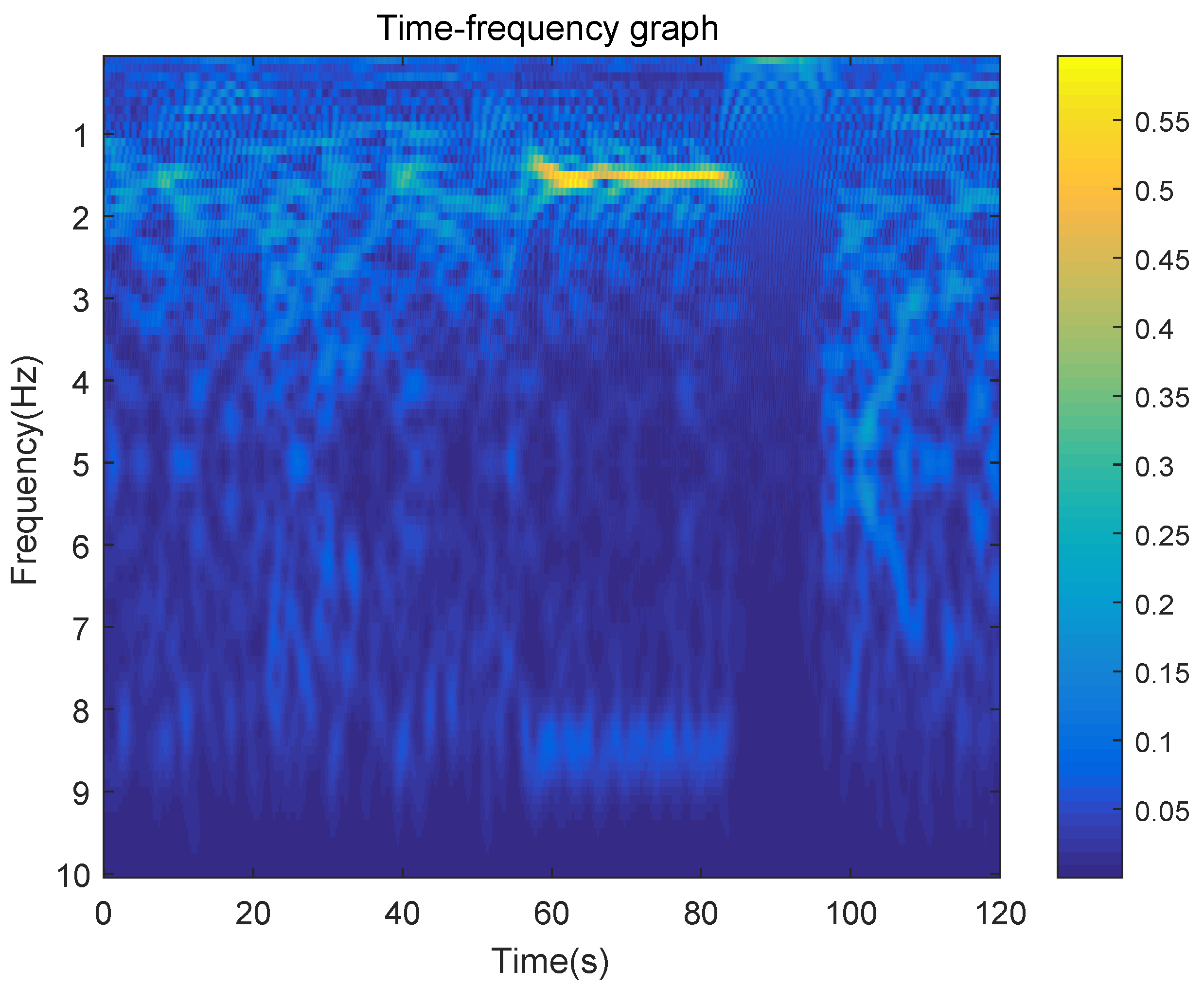
In order to verify the effectiveness of wavelet transform in diagnosing surge in the above conclusions, the outlet flow signal at 40,000 rpm is subjected to wavelet transform with the same wavelet parameters and algorithms, and the result is shown in Figure 12. By comparing Figure 11 and Figure 12, it can be obviously seen that the dominant frequency of the outlet flow signal collected at 20,000 rpm and 40,000 rpm during surge are basically the same, and both are about 1.4 Hz. For the same centrifugal air compressor, the characteristic frequencies of surge flow at different speeds are similar. Based on this assumption, we can judge whether the centrifugal air compressor has surge by studying the most obvious series of wavelet coefficient values in the wavelet coefficient graph.

4.2. Data Post-Processing

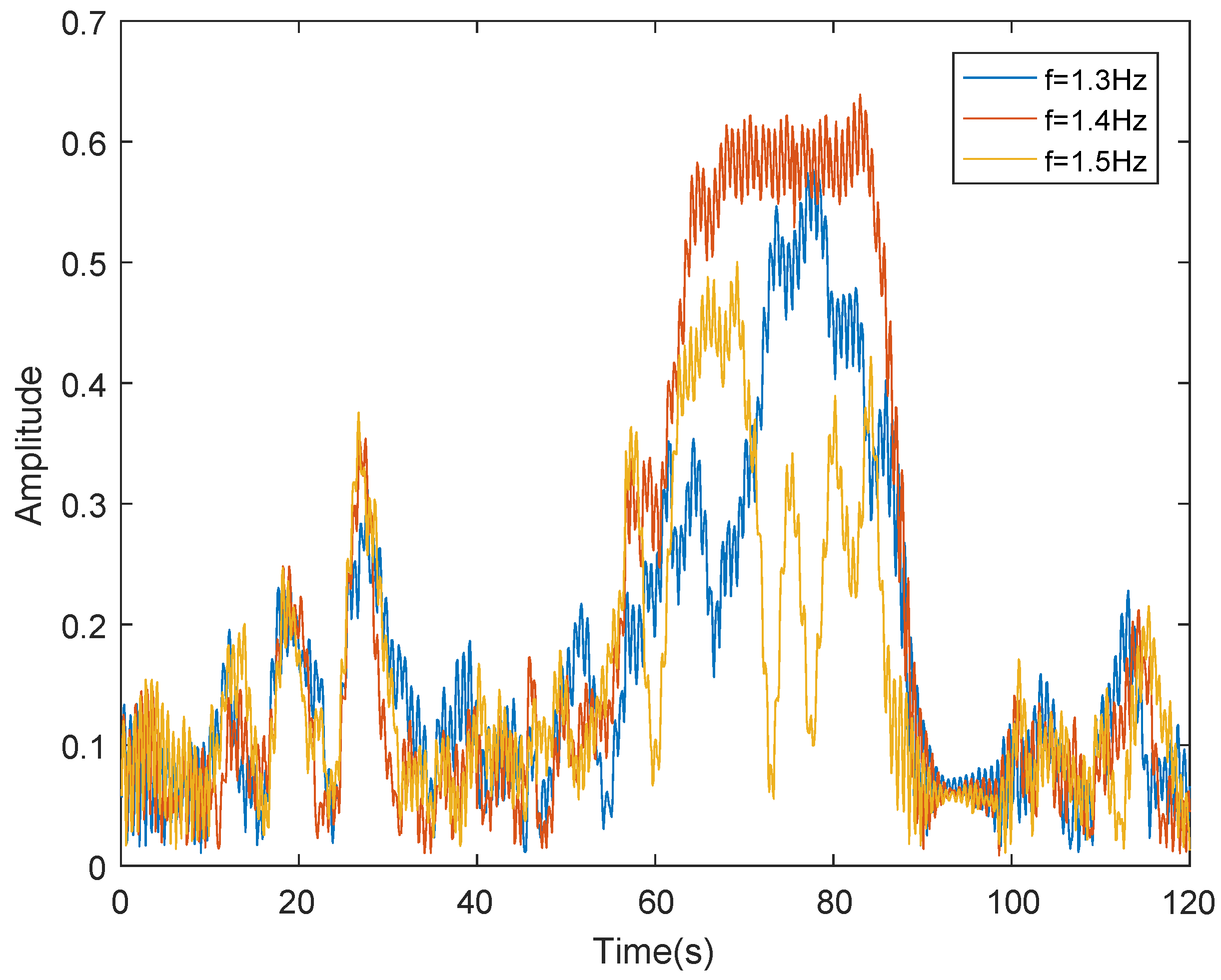
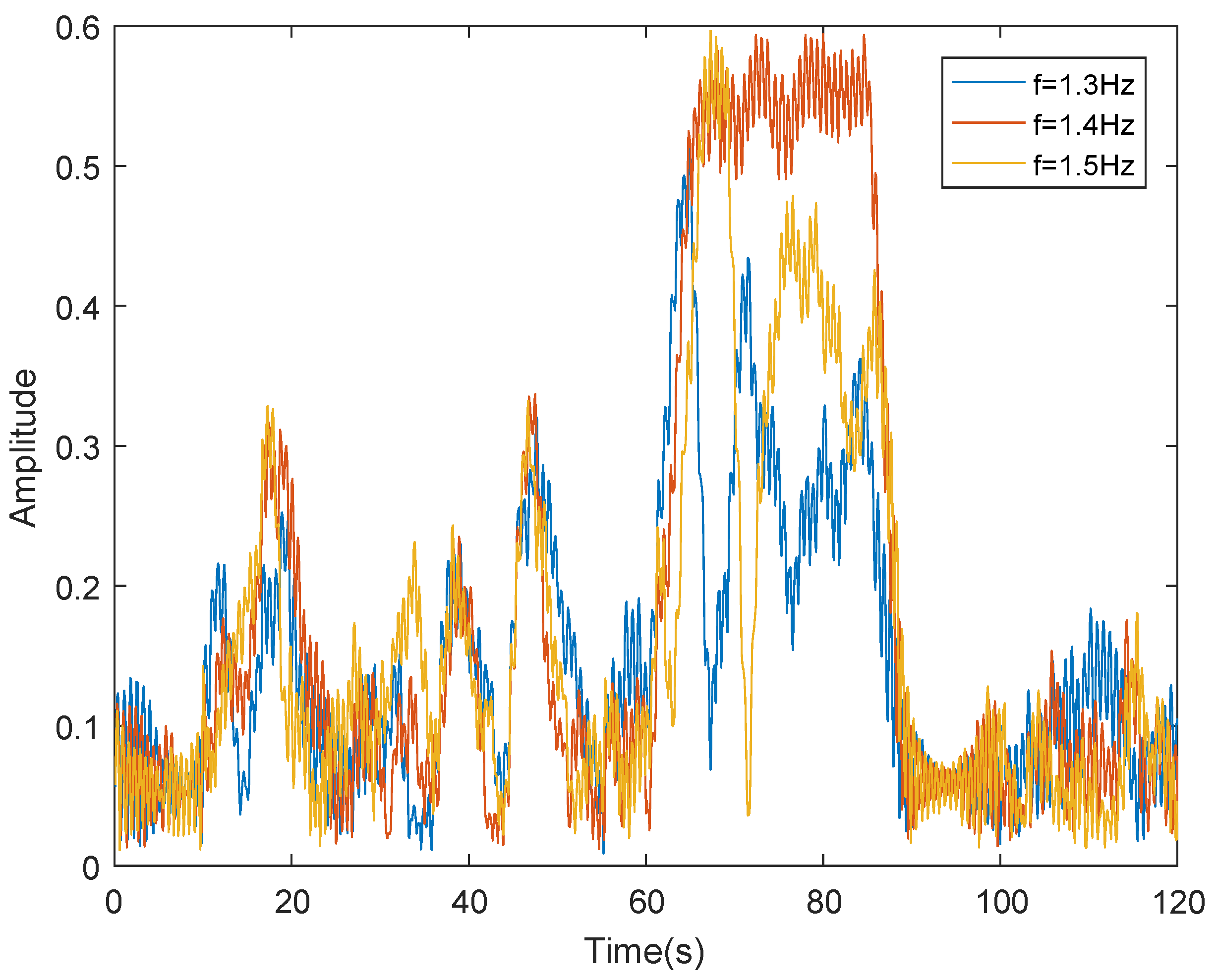
In engineering applications, if a large frequency range (0–10 Hz) wavelet transform is performed on the outlet flow signal according to the traditional method, it will cause calculation delay and waste of memory. The analysis results of the above Fourier transform and wavelet transform show that the dominant frequency of the outlet flow of the centrifugal air compressor during surge is about 1.4 Hz, so the wavelet coefficients of a certain scale parameter can be selected as the research object. In order to obtain more accurate scale parameters with obvious changes in wavelet coefficients, the wavelet coefficients at 1.3 Hz, 1.4 Hz and 1.5 Hz are taken for analysis. The wavelet transform results at 20,000 rpm and 40,000 rpm are shown in Figure 13 and Figure 14.

In Figure 13 and Figure 14, we can see that in the quasi-surge region, that is, before 60 s, the amplitude of the wavelet coefficients obtained by the above three scale parameters are almost the same, and the maximum values are all below 0.4, which means the energy is small. In the surge region, that is, after 60 s, the wavelet coefficients show obvious differences. Except for the amplitude of the wavelet coefficients corresponding to 1.4 Hz, which has a large and stable value, the data of 1.3 Hz and 1.5 Hz fluctuates drastically. The later two value ranges touch the quasi-surge zone, and it is impossible to clearly distinguish between the quasi-surge and surge zone. The highest amplitude contrast is the 1.4 Hz data, which has a generally higher value in the surge area, while the fluctuation amplitude is small, and all the data are above 0.5.

When we use the variable limit flow method to control the anti-surge of the centrifugal air compressor, the judgment threshold can be set in the quasi-surge area or the surge area. For the method of setting the wavelet coefficient amplitude threshold in the quasi-surge zone, it can detect the trend of surge in time, and execute the anti-surge strategy before the actual occurrence of surge. However, the disadvantage is that when the more extreme centrifugal air compressor control algorithm is applied, it is close to the quasi-surge area and falsely triggers the anti-surge strategy, resulting in a waste of energy. As for the method of setting the wavelet coefficient amplitude threshold in the surge zone, the anti-surge strategy is executed only when surge is really to occur. The disadvantage is that it will cause certain damage to the air compressor. Therefore, in practical applications, the quasi-surge zone threshold or the surge zone threshold should be used according to the user’s choice of anti-surge strategy.

In this paper, the second threshold selection method is adopted, and 0.4 is taken as the judgment threshold of the anti-surge strategy. For 20,000 rpm, the maximum wavelet coefficient amplitude of the quasi-surge zone is 0.3556, and there is a 10% safety margin to prevent the anti-surge strategy from being falsely triggered during the quasi-surge. As for 40,000 rpm, there is 16% safety margin.

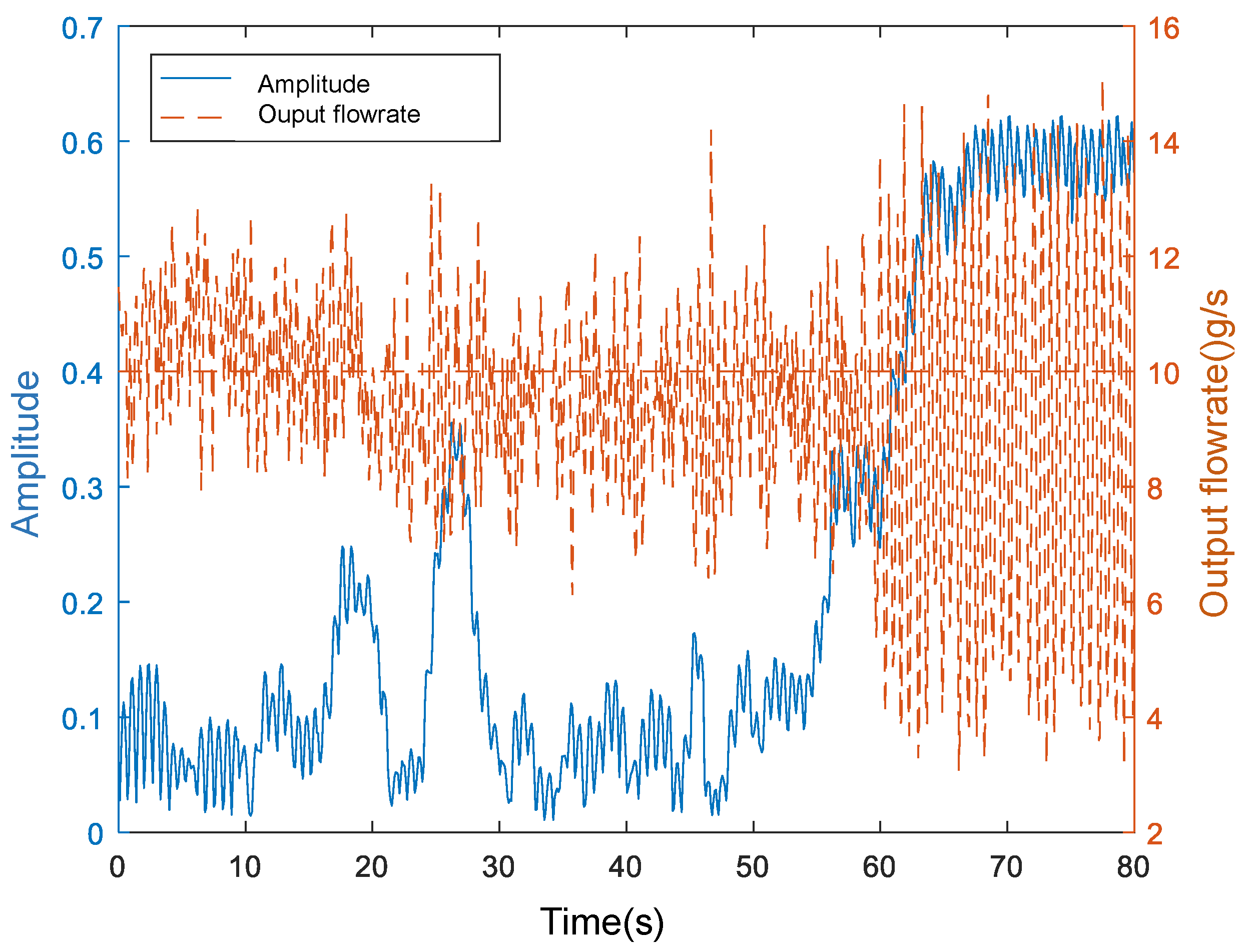
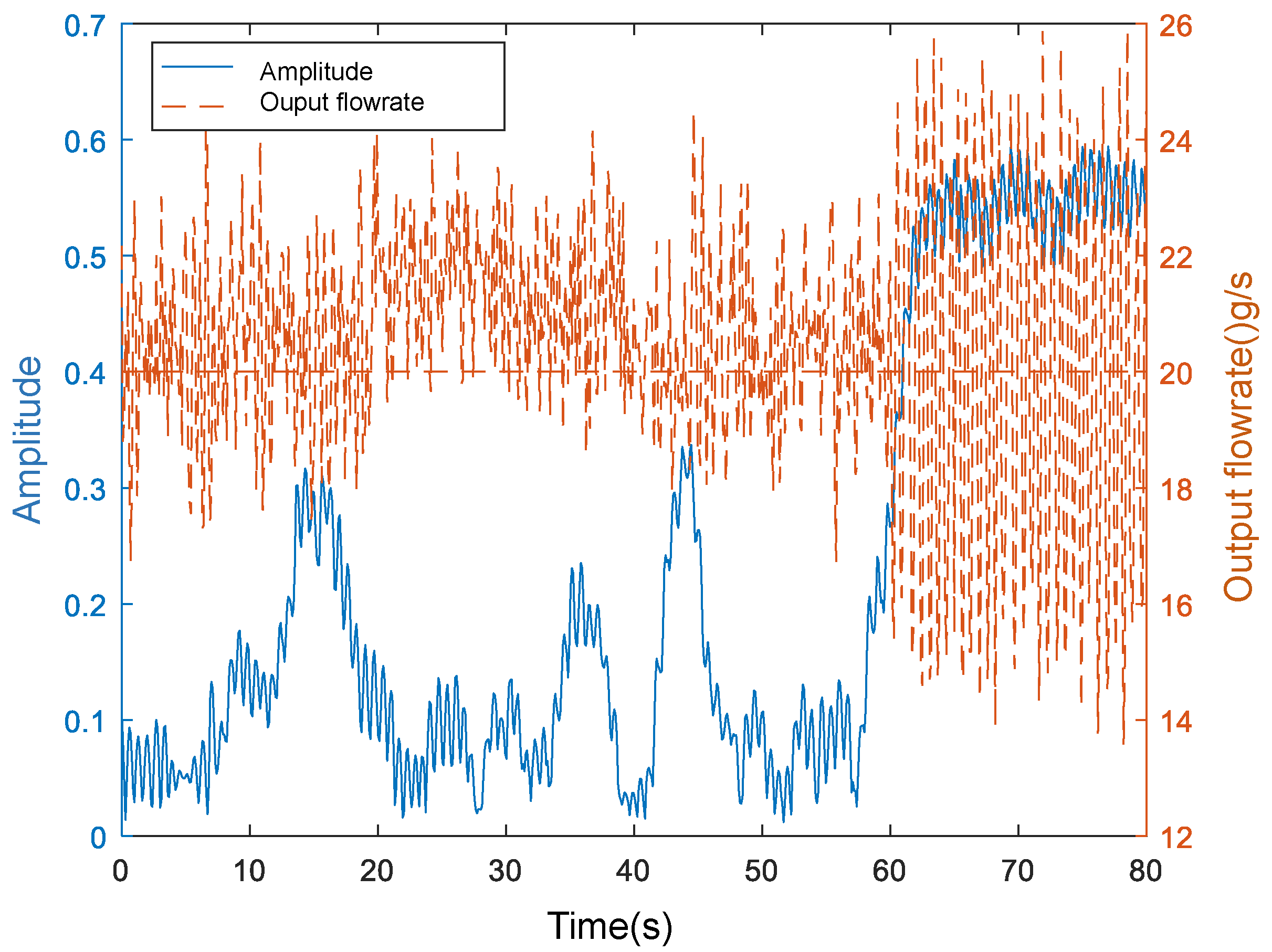
Putting the original flow data and the 1.4 Hz wavelet coefficient amplitude on the same graph for observation, as shown in Figure 15 and Figure 16, it can be seen that the wavelet coefficients all reach the above-determined surge threshold in about 61 s (61.1 s and 61.3 s, respectively). It is judged that the surge occurs near this point in time, and the flow fluctuation degree has been very big. Therefore, the method in this paper can detect the occurrence of surge in time, and provide a judgment basis for anti-surge control.

5. Conclusions

Centrifugal air compressors are prone to surge under small flow and high pressure ratio conditions, which will cause permanent damage to the impeller. A real-time online diagnosis method based on wavelet transform designed in this paper can effectively detect whether the centrifugal air compressor has a tendency to surge. This paper analyzes the collected flow at different speeds by Fourier transform, and obtains the hypothesis that the surge flow at different speeds of the centrifugal air compressor has similar characteristic frequencies. Based on this this assumption, we performed the complex Morlet wavelet transform on a section of flow signal including surge failure of the air compressor. The test results show that at the characteristic frequency of outlet flow, the wavelet coefficient will have a huge change when the surge failure is about to occur. This discovery has inspired us to use only the wavelet coefficients at the characteristic frequency and compare it with a certain threshold, which can prevent the occurrence of surge faults, and this approach has greatly improved the calculation speed of diagnosis and saved calculation memory.

However, when using the wavelet transform method for air compressor surge monitoring, only the air compressor flow is considered, and other factors such as temperature and noise are not considered. If these interference factors can be considered together, the monitoring method will be more precise.

The method based on wavelet analysis proposed in this paper is a novel method that is different from traditional flow rate monitoring in anti-surge field to a certain extent, and its effectiveness has been temporarily verified. However, there are still shortcomings. In addition to the above-mentioned accuracy problems, in fact, the bigger challenge is that if we want to promote this method in engineering applications, we need to calibrate a wavelet coefficient threshold curve, which is very similar to the limit flow threshold curve in Figure 2 and Figure 3. In addition, this paper does not prove whether this diagnostic method is still effective when the system pipeline changes and the air compressor is aging because, in that case, the threshold and the characteristic frequency may also drift. These need our follow-up research to be confirmed.

References

- Larminie, J.; Dicks, A.; McDonald, M.S. Fuel Cell Systems Explained; J. Wiley Chichester: Chichester, UK, 2003; Volume 2. [Google Scholar]
- Priya, K.; Sathishkumar, K.; Rajasekar, N. A comprehensive review on parameter estimation techniques for Proton Exchange Membrane fuel cell modelling. Renew. Sustain. Energy Rev. 2018, 93, 121–144. [Google Scholar] [CrossRef]
- Nistor, S.; Dave, S.; Fan, Z.; Sooriyabandara, M. Technical and economic analysis of hydrogen refuelling. Appl. Energy 2016, 167, 211–220. [Google Scholar] [CrossRef]
- Wee, J.H. Applications of proton exchange membrane fuel cell systems. Renew. Sustain. Energy Rev. 2007, 11, 1720–1738. [Google Scholar] [CrossRef]
- Zhou, S.; Chen, F. PEMFC System Modeling and Control. Adv. Chem. Eng. 2012, 41, 197–263. [Google Scholar]
- Pukrushpan, J.T.; Stefanopoulou, A.G.; Peng, H. Fuel Cell System Model: Analysis and Simulation. In Control of Fuel Cell Power Systems: Principles, Modeling, Analysis and Feedback Design; Springer: London, UK, 2004; pp. 57–64. [Google Scholar] [CrossRef]
- Danzer, M.A.; Wilhelm, J.; Aschemann, H.; Hofer, E.P. Model-based control of cathode pressure and oxygen excess ratio of a PEM fuel cell system. Selected Papers Presented at the10th ULM ElectroChemical Days. J. Power Sour. 2008, 176, 515–522. [Google Scholar] [CrossRef]
- Blunier, B.; Miraoui, A. Proton Exchange Membrane Fuel Cell Air Management in Automotive Applications. J. Fuel Cell Sci. Technol. 2010, 7, 1571–1574. [Google Scholar] [CrossRef]
- Liu, Z.; Li, L.; Ding, Y.; Deng, H.; Chen, W. Modeling and control of an air supply system for a heavy duty PEMFC engine. Special Issue: 16th China Hydrogen Energy Conference (CHEC 2015), November 2015, Zhenjiang City, Jiangsu Province, China. Int. J. Hydrog. Energy 2016, 41, 16230–16239. [Google Scholar] [CrossRef]
- Blunier, B.; Cirrincione, G.; Hervé, Y.; Miraoui, A. A new analytical and dynamical model of a scroll compressor with experimental validation. Int. J. Refrig. 2009, 32, 874–891. [Google Scholar] [CrossRef]
- Zhao, D.; Dou, M.; Blunier, B.; Miraoui, A. Control of an ultra high speed centrifugal compressor for the air management of fuel cell systems. In Proceedings of the 2012 IEEE Industry Applications Society Annual Meeting, Las Vegas, NV, USA, 7–11 October 2012; pp. 1–8. [Google Scholar]
- Xue, X.; Wang, T.; Zhang, T.; Yang, B. Mechanism of stall and surge in a centrifugal compressor with a variable vaned diffuser. Chin. J. Aeronaut. 2018, 31, 1222–1231. [Google Scholar] [CrossRef]
- Shahin, I.; Alqaradawi, M.; Gadala, M.; Badr, O. Large eddy simulation of surge inception and active surge control in a high speed centrifugal compressor with a vaned diffuser. Appl. Math. Model. 2016, 40, 10404–10418. [Google Scholar] [CrossRef]
- Huang, Q.; Zhang, M.; Zheng, X. Compressor surge based on a 1D–3D coupled method—Part 1: Method establishment. Aerosp. Sci. Technol. 2019, 90, 342–356. [Google Scholar] [CrossRef]
- Khaleghi, H. Stall inception and control in a transonic fan, part B: Stall control by discrete endwall injection. Aerosp. Sci. Technol. 2015, 41, 151–157. [Google Scholar] [CrossRef]
- Righi, M.; Pachidis, V.; Könözsy, L.; Pawsey, L. Three-dimensional through-flow modelling of axial flow compressor rotating stall and surge. Aerosp. Sci. Technol. 2018, 78, 271–279. [Google Scholar] [CrossRef]
- Tian, C. Anti-surge Control of Centrifugal Compressor. Petrochem. Ind. Technol. 2007, 14, 44–46. [Google Scholar]
- Qin, J.; Du, J. Scheme of Antisurge Control for Centrifugal Compressor. Autom. Panor. 2005, 22, 38–39. [Google Scholar]
- Hou, W. Inquire into C3000 Applied in the Centrifugal Air Compressor Antisurge. In Automation in Petrochemical Industry; Valmet: Espoo, Finland, 2009; pp. 79–82. [Google Scholar]
- Cortinovis, A.; Ferreau, H.; Lewandowski, D.; Mercangöz, M. Experimental evaluation of MPC-based anti-surge and process control for electric driven centrifugal gas compressors. J. Process. Control 2015, 34, 13–25. [Google Scholar] [CrossRef]
- Bøhagen, B.; Gravdahl, J.T. Active surge control of compression system using drive torque. Automatica 2008, 44, 1135–1140. [Google Scholar] [CrossRef] [Green Version]
- Liu, A.; Zheng, X. Methods of surge point judgment for compressor experiments. Exp. Therm. Fluid Sci. 2013, 51, 204–213. [Google Scholar] [CrossRef]
- Galindo, J.; Tiseira, A.; Arnau, F.; Lang, R. On-engine measurement of turbocharger surge limit. Exp. Tech. 2013, 37, 47–54. [Google Scholar] [CrossRef] [Green Version]
- Liu, X.; Zhao, L. Approximate Nonlinear Modeling of Aircraft Engine Surge Margin Based on Equilibrium Manifold Expansion. Chin. J. Aeronaut. 2012, 25, 663–674. [Google Scholar] [CrossRef] [Green Version]
- Javadi Moghaddam, J.; Farahani, M.; Amanifard, N. A neural network-based sliding-mode control for rotating stall and surge in axial compressors. Appl. Soft Comput. 2011, 11, 1036–1043. [Google Scholar] [CrossRef]
- Javadi Moghaddam, J.; Madani, M. A decoupled adaptive neuro-fuzzy sliding mode control system to control rotating stall and surge in axial compressors. Expert Syst. Appl. 2011, 38, 4490–4496. [Google Scholar] [CrossRef]
- Li, F.; Li, S.; Chenli, S.; Feng, Q. Research and Application of Anti-surge Control and Fault Diagnosis System to Centrifugal Compressor. Control Inst. Chem. Ind. 2011, 38, 589–592. [Google Scholar]
- Sun, Z.; Zheng, X.; Tamaki, H.; Kaneko, Y. Flow instability suppression and deep surge delay by non-axisymmetric vaned diffuser in a centrifugal compressor. Aerosp. Sci. Technol. 2019, 95, 105494. [Google Scholar] [CrossRef]
- Hoshi, Y.; Yakabe, N.; Isobe, K.; Saito, T.; Shitanda, I.; Itagaki, M. Wavelet transformation to determine impedance spectra of lithium-ion rechargeable battery. J. Power Sources 2016, 315, 351–358. [Google Scholar] [CrossRef]
- Itagaki, M.; Ueno, M.; Hoshi, Y.; Shitanda, I. Simultaneous determination of electrochemical impedance of Lithium-ion rechargeable batteries with measurement of charge-discharge curves by wavelet transformation. Electrochim. Acta 2017, 235, 384–389. [Google Scholar] [CrossRef]
- Grinsted, A.; Moore, J.C.; Jevrejeva, S. Application of the cross wavelet transform and wavelet coherence to geophysical time series. Nonlinear Process. Geophys. 2004, 11, 561–566. [Google Scholar] [CrossRef]
- Torrence, C.; Compo, G.P. A practical guide to wavelet analysis. Bull. Am. Meteorol. Soc. 1998, 79, 61–78. [Google Scholar] [CrossRef] [Green Version]
- Lin, J.; Qu, L. Feature extraction based on Morlet wavelet and its application for mechanical fault diagnosis. J. Sound Vib. 2000, 234, 135–148. [Google Scholar] [CrossRef]
- Cheng, F.B.; Tang, B.P.; Zhong, Y.M. A de-noising method based on optimal Morlet wavelet and singular value decomposition and its application in fault diagnosis. J. Vib. Shock 2008, 2, 91–94. [Google Scholar]
- Ding, L.; Zeng, R.; Shen, H.; Zhao, H.; Zeng, R. An engine fault diagnosis method based on Shannon entropy features. J. Vib. Shock 2018, 37, 241–247. [Google Scholar]
- Tang, X.; Li, Q. Time-Frequency Analysis and Wavelet Transform; Science Press: Beijing, China, 2008. [Google Scholar]
- Pan, Z.; Liang, S.; Li, J.; Liu, Y. Application of the complex wavelet analysis in fault feature extraction of blower rolling bearing. Proc. CSEE 2015, 35, 4147–4152. [Google Scholar]
Figure 1.
The structure of PEM fuel cell system.
Figure 2.
Fixed limit flow method.
Figure 3.
Variable limit flow method.
Figure 4.
The influence of parameters a and b on the position and shape of wavelet function.
Figure 5.
Effect of on complex Morlet mother wavelet at Hz (solid line, real part; dotted line, imaginary part.
Figure 6.
The air compressor test bench.
Figure 7.
Diagram of centrifugal air compressor test bench.
Figure 8.
Outlet flow rate of centrifugal air compressor (@20,000 rpm/@40,000 rpm).
Figure 9.
Outlet pressure of centrifugal air compressor (@20,000 rpm/@40,000 rpm).
Figure 10.
Results of Fourier transform.
Figure 11.
Wavelet coefficients (@20,000 rpm).
Figure 12.
Wavelet coefficients (@40,000 rpm).
Figure 13.
Wavelet coefficients as f = 1.3/1.4/1.5 (@20,000 rpm).
Figure 14.
Wavelet coefficients as f = 1.3/1.4/1.5 (@40,000 rpm).
Figure 15.
Wavelet coefficients and original flowrate data (@20,000 rpm).
Figure 16.
Wavelet coefficients and original flowrate data (@40,000 rpm).
Publisher’s Note: MDPI stays neutral with regard to jurisdictional claims in published maps and institutional affiliations. |
© 2021 by the authors. Licensee MDPI, Basel, Switzerland. This article is an open access article distributed under the terms and conditions of the Creative Commons Attribution (CC BY) license (https://creativecommons.org/licenses/by/4.0/).
Share and Cite
MDPI and ACS Style
Zhou, S.; Jin, J.; Wei, Y. Research on Online Diagnosis Method of Fuel Cell Centrifugal Air Compressor Surge Fault. Energies 2021, 14, 3071. https://doi.org/10.3390/en14113071
AMA Style
Zhou S, Jin J, Wei Y. Research on Online Diagnosis Method of Fuel Cell Centrifugal Air Compressor Surge Fault. Energies. 2021; 14(11):3071. https://doi.org/10.3390/en14113071
Chicago/Turabian StyleZhou, Su, Jie Jin, and Yuehua Wei. 2021. "Research on Online Diagnosis Method of Fuel Cell Centrifugal Air Compressor Surge Fault" Energies 14, no. 11: 3071. https://doi.org/10.3390/en14113071
Note that from the first issue of 2016, this journal uses article numbers instead of page numbers. See further details here.