
Neural Networks in the Diagnostics Process of Low-Power Solar Plant Devices
by
 , ,
, ,
Stanisław Duer
1,*, 
Jan Valicek
2,
Jacek Paś
3 ,
,
Marek Stawowy
4,
Dariusz Bernatowicz
5,
Radosław Duer
5 and
Marcin Walczak
5 1
Department of Energy, Faculty of Mechanical Engineering, Technical University of Koszalin, 15–17 Raclawicka St., 75-620 Koszalin, Poland
2
Department of Electrical Engineering, Automation and Informatics, Faculty of Engineering, Slovak University of Agriculture in Nitra, Tr. A. Hlinku 2, 94976 Nitra, Slovakia
3
Faculty of Electronic, Military University of Technology of Warsaw, 2 Urbanowicza St., 00-908 Warsaw, Poland
4
Department of Transport Telecommunication, Faculty of Transport, Warsaw University of Technology, Koszykowa St. 75, 00-662 Warsaw, Poland
5
Faculty of Electronics and Computer Science, Technical University of Koszalin, 2 Sniadeckich St., 75-620 Koszalin, Poland
*
Author to whom correspondence should be addressed.
Energies 2021, 14(9), 2719; https://doi.org/10.3390/en14092719
Submission received: 12 March 2021
/
Revised: 2 May 2021
/
Accepted: 6 May 2021
/
Published: 10 May 2021
(This article belongs to the Special Issue Challenge and Research Trends of Artificial Neural Network)
Abstract
:The article presents the problems of diagnostics of low-power solar power plants with the use of the three-valued (3VL) state assessment {2, 1, 0}. The 3VL diagnostics is developed on the basis of two-valued diagnostics (2VL), and it is elaborated on. In the (3VL) diagnostics, the range of changes in the values of the signals from the 2VL logic was accepted for the serviceability condition: state {12VL}. This range of signal value changes for logic (3VL) was divided into two signal value change sub-ranges, which were assigned two status values in the logic (3VL): {23VL}—serviceability condition and {13VL}—incomplete serviceability condition. The state of failure for both logics applied of the valence of states is interpreted equally for the same changes in the values of diagnostic signals, the possible changes of which exceed the ranges of their permissible changes. The DIAG 2 intelligent system based on an artificial neural network was used in diagnostic tests. For this purpose, the article presents the structure, algorithm and rules of inference used in the DIAG intelligent diagnostic system. The diagnostic method used in the DIAG 2 system utilizes the method known from the literature to compare diagnostic signal vectors with the reference signal vectors assigned. The result of this vector analysis is the metric developed of the difference vector. The problem of signal analysis and comparison is carried out in the input cells of the neural network. In the output cells of the neural network, in turn, the classification of the states of the object’s elements is realized. Depending on the condition of the individual elements that make up the object, the method is able to indicate whether the elements are in working order, out of order or require quick repair/replacement.
1. Introduction
Artificial intelligence systems including neural networks are extensively elaborated on in the literature, particularly in the studies [1,2,3,4,5,6,7]. These studies constitute a sufficient compendium of knowledge concerning the principle of the functioning of artificial neural networks. They also contain biological and mathematical bases of the structure and functioning of the single neuron and the neural network. The authors described well the theoretical bases of the construction of static neural networks, and ways of teaching and training them. These studies can be useful when designing artificial neural networks that function based on radial base functions, including their structures, teaching and practice [4,5]. The authors also made great efforts drawing up chapters concerning dynamic neural networks, principles of their construction, teaching and training. A significant part of these studies concerns the use of sets and fuzzy knowledge in the functioning of artificial neural networks [8,9,10,11].
The papers [12,13,14,15,16,17,18] constitute the first item in the references. They cover the theory of the operation of technical devices. They include a mathematical description of a model of a technical object as regards its reliability and operation. The papers also present an organization of the operation process with the use of the object’s models presented. The authors also possess a lot of experience in diagnostic testing of technical devices, the effect of which is their previous studies.
In recent years, the direction of technical diagnostics in particular has been intensively developed with the application of artificial intelligence systems, including artificial neural networks. A number of different aspects, which take into consideration the complexity of the controlling process of industrial robots of different types and an adjustment of technological systems, are taken into account in the research concerning controlling and diagnosing systems of technical and technological processes [16,17,18,19,20,21,22,23,24,25,26,27,28,29,30].
The studies [2,10,11] may be of great practical significance in the organization of a diagnostic system with the use of artificial neural networks. In these studies, a method was presented that shows a practical use of the results of technical diagnostics in the organization of a technical object operation system. In the research, an idea was presented concerning a change in states in a technical object. As a result of it, there is a decrease of its functional properties, i.e., a change in the state. Therefore, there occurs a necessity of an effective diagnosis of this ensuing state in the object. In the case when the state diagnosed is the state of an incomplete operable condition or non-operable condition, appropriate counteraction is to be undertaken through the organization of prevention (a regeneration of the object). In the aforementioned studies, the authors presented a diagram and a description of the structure of an artificial neural network as well as theoretical dependencies that describe the functioning of the network in accordance with the algorithm presented therein. The theoretical bases concerning diagnosing of technical objects were also presented in the trivalent logic with the use of an artificial neural network. The results of the study were supported with an example of setting up of a diagnostic information base for the device under examination [31,32].
In the diagnostics of technical objects, the object of action is the object itself. Its purpose, structure and specificity of functioning impose (define) the method of diagnosis. The problem of diagnosis described in this work concerns a complex technical object. The paper presents the specificity of the construction and operation of these types of solar power plant devices. A novelty in this article in the aspect of solar low-power plant devices (L-PPD) is a presentation of the method of building and developing diagnostic knowledge bases for the (L-PPD).
The authors of the article systematically improved the reliability condition testing of technical devices by improving the method of testing the condition of the object, consisting of an analysis of distance metrics resulting from a comparison of diagnostic signal vector images with their patterns. For this purpose, solutions developed on the basis of artificial intelligence and expert systems were used. The result of this work is a diagnostic computer program: DIAG 2 [11,31,32,33,34].
In the literature, the experiments and research results of solar low-power plant devices are presented in the following works [35,36,37,38,39,40]. In the article by Hwang et al. [34], multilayer neural networks (MNN) were adopted for diagnostics of solar panels of solar street lamps. The network type that was used was based on adaptive resonance theory 2 (ART2). The voltage was applied in the duty cycle from unloaded panels as data to the two neural networks. The paper by Ganeshprabu et al. [36] employs a distributed on-line monitoring system based on the XBee wireless sensor network to monitor the operating parameters of photovoltaic panels, such as the output current, voltage and module insolation, temperature and environmental insolation. The paper by Jiang et al. [37] presents a method of automatic detection and diagnostics of faults in photovoltaic (PV) systems. It combines an artificial neural network (ANN) with a conventional analytical method for fault detection and diagnosis. A two-layer ANN network was used for power prediction. On the basis of the difference between projected power and measured power, the open-circuit voltage and short-circuit current of a PV module string that is determined by analytical equations, the authors identify up to six defined fault types.
The article by Duer et al. [38] describes research issues related to two- and three-valued logical diagnoses developed with the use of a diagnostic system (DIAG 2) for devices installed in a low-power substation. The paper also briefly presents the intelligent diagnostic system (DIAG 2) used for the tests presented here. The diagnostic system (DIAG 2) works by comparing a set of actual diagnostic output vectors with their main vectors. The result of the comparison is elementary divergence metrics of diagnostic output vectors determined by the neural network. Elementary divergence metrics include differential distance metrics that serve as input (DIAG 2) to compute the state of the basic elements of the test object. Predicting the output power of various types of photovoltaic cells was the main task of Artificial Neural Network (ANN) modeling in [39]. The method was used for three types of cells: mono-crystalline (mono-), multi-crystalline (multi-), and amorphous (amor-) crystalline. The results show the following order of efficiency in electricity production: multi-, mono- and amor-crystalline cell types. Diagnostics of damage to photovoltaic (PV) panels was the main topic of the article [40]. The presented method is based on the analysis of the optimal characteristics of a fault on the basis of current-voltage (I–V) curves from various faults, including hybrid faults. In addition, a deterministic algorithm for the reflective confidence region was proposed in combination with a metaheuristic algorithm for particle swarm optimization (PSO) to standardize the fault characteristics. Additionally, the multiclass adaptive enhancement algorithm (AdaBoost) was used, which is a stagewise additive modeling using the multiclass exponential loss function (SAMME) based on the classification and regression tree (CART).
The article presents the problem of diagnosing of low-power solar plant devices (a complex technical object) with the use of three-valued state evaluation (3VL). The problem of diagnostics in three-state assessment has been developed intensively in the past 10 to 20 years. The basis for the development of three-valued diagnostics, as well as of two-valued diagnostics, was the theory of three-state logic developed by J. Łukasiewicz, 1920. For this diagnostics, Duer [33,34,35] is known in the literature. Three-state diagnostics {2, 1, 0} differs from two-state diagnostics in the third state, i.e., state “1”, which is interpreted in it. The “1” condition is referred to in the literature as an incomplete condition [2,10,11]. The article consists of four main chapters. The second chapter of the article presents the diagnostic algorithm implemented in the DIAG intelligent diagnostic system. It presents the diagnostic method used, which consists of comparing the diagnostic signal vectors with the appropriate model diagnostic signal vector assigned to them. At this stage of diagnosis, the metric of the vector divergence vector is determined. This first stage of the diagnosis algorithm is implemented in the input cells of the neural network. The main stage of diagnostics is performed in the output cells of the neural network. These cells classify the states of the basic elements in the object on the basis of an analysis of the vector divergence vector and assign it to one of the possible range changes in the value of signal metrics. The third chapter describes the method of classifying states for fundamental elements. In the output cells of the neural network, the states of the basic elements in the object are classified on the basis of an analysis of the vector divergence vector and its assignment to one of the possible interval changes in the values of signal metrics. The fourth chapter presents a practical verification of the diagnostic method presented with the use of an artificial neural network in the DIAG program for low-power solar plant devices (L-PSPD).
2. The Algorithm and Structure of an Artificial Neural Network SBM in the Program of DIAG Intelligent Diagnosis System
The comparison method of images presented in the study constitutes in a general sense a representation of a wider theory that is known in the literature as the theory of image recognition presented in the studies (Tadeusiewicz and Korohoda, 1997) [10]. Those methods that describe the types of the transformations information used in a given moment of the image recognition theory are of different types. The following are the most frequently applied transformations: the Fourier transform, the Gabor transform and the wavelet transform as well as the Hough transform (describing a detection of straight lines). The above solutions are justifiable and require their use during the transformations of images with a great complexity (integration). In the case of simple images that describe, e.g., a diagnostic signal in a vector form in the k-surface space that describes k-features of the diagnostic signal. For analogue sinusoidal signals, the continuous features of the signal are the amplitude, the repetition period, the pulsation (the angular velocity of the phase change) and the initial phase. In such a situation, the methods used in practice that identify images are considerably simpler. The metric measures of the determination of the conformity of similarity of the image identified with its standard image belong to these methods.
The literature includes a description of a wide group of the methods of neural networks that realize the task of the determination of the similarity of objects, or a group of neural networks that qualifies objects with certain distinguished features for the class as specified for them. Both groups of methods are very similar to one another concerning the functions realized. These network methods are frequently used interchangeably, e.g., networks from the group of “similarity assessment” with the group of the networks of “nearest neighbors” in the case of a required complementation, comparison of the quality of operation, etc. The “nearest neighbors” method has numerous applications in the identification of standards or otherwise in the time of a generalization of the features of an object that are described in a multidimensional space, and these are networks known as pattern recognition [1,2,3,4,5,10].
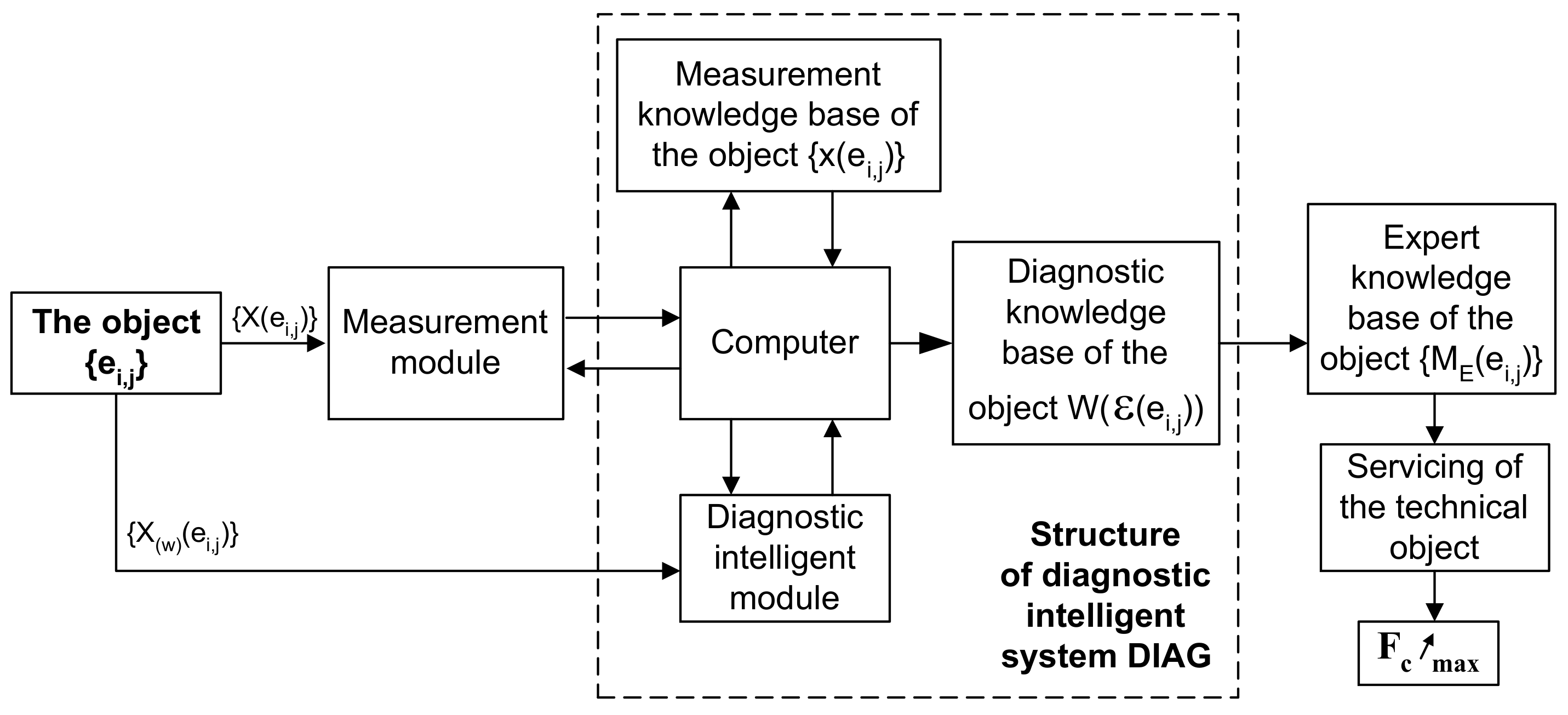
In the diagnostics of technical objects, the methods of neural networks can be used based on similarity, known as the networks of the type of similarity-based methods SBM (Figure 1). In the literature, information is provided that the theory of similarity developed independently from the development of neural networks as such and the development of other methods applied in the problems of qualification. No such characterization of data was found that would allow determining which method should be selected (applied) and which methods would be most suitable for their qualification. Each of those researchers who examine the reality in their scope of interests suitably to their needs proposes specific methods that guarantee to him/her specific results and their quality.
In the diagnostics of technical objects, the method of comparing diagnostic signals with their model signals is commonly used. This diagnostic method is presented in the literature [2,10,31,32,33,34] in the form of the following equation:
where the following stand for: W(ε(ei,j)) is the value of state assessment logics for jth element within ith module, X(ei,j) is the diagnostic signal in jth element of ith assembly of the object, X(w)(ei,j) is the model signal for X(ei,j) signal, is a symbol of diagnostic activities, Ei is the ith assembly of the object, is a symbol of comparison.
The majority of methods applied that determine similarity-based methods SBM originate from distance measurements (metric measures of distance measurements). This transformation is realized with the use of the determined (sought) weighting function, which sets the measure of similarity. In the studies of (Duch and Jankowski, 1999) [10], it was presented that good results are obtained for minimum distance methods using the Euclidean metric for given continuous data, or the Hamming measure for binary data. Additional parameters that may be subject to optimization are either centrally–globally (the same in the whole space) or locally (different for each reference vector). The distance metric most frequently used from among neural network methods is Minkowski’s measure, which possesses one global adaptation parameter (α) for (α = 2, this is Euclidean measure), while for (α = 1, this is Manhattan measure).
In the process of modeling artificial neural networks, the relationship developed by Minkowski is used with the (α = 2) condition in the form of the equation:
where the following stand for:
- DM(Xi, X(w)i α) is the standard deviation of the vector the signal metric, (α = 2),
- X(ei,j) is the diagnostic signal in jth element of ith set,
- X(w)(ei,j) is the model signal for X(ei,j) signal.
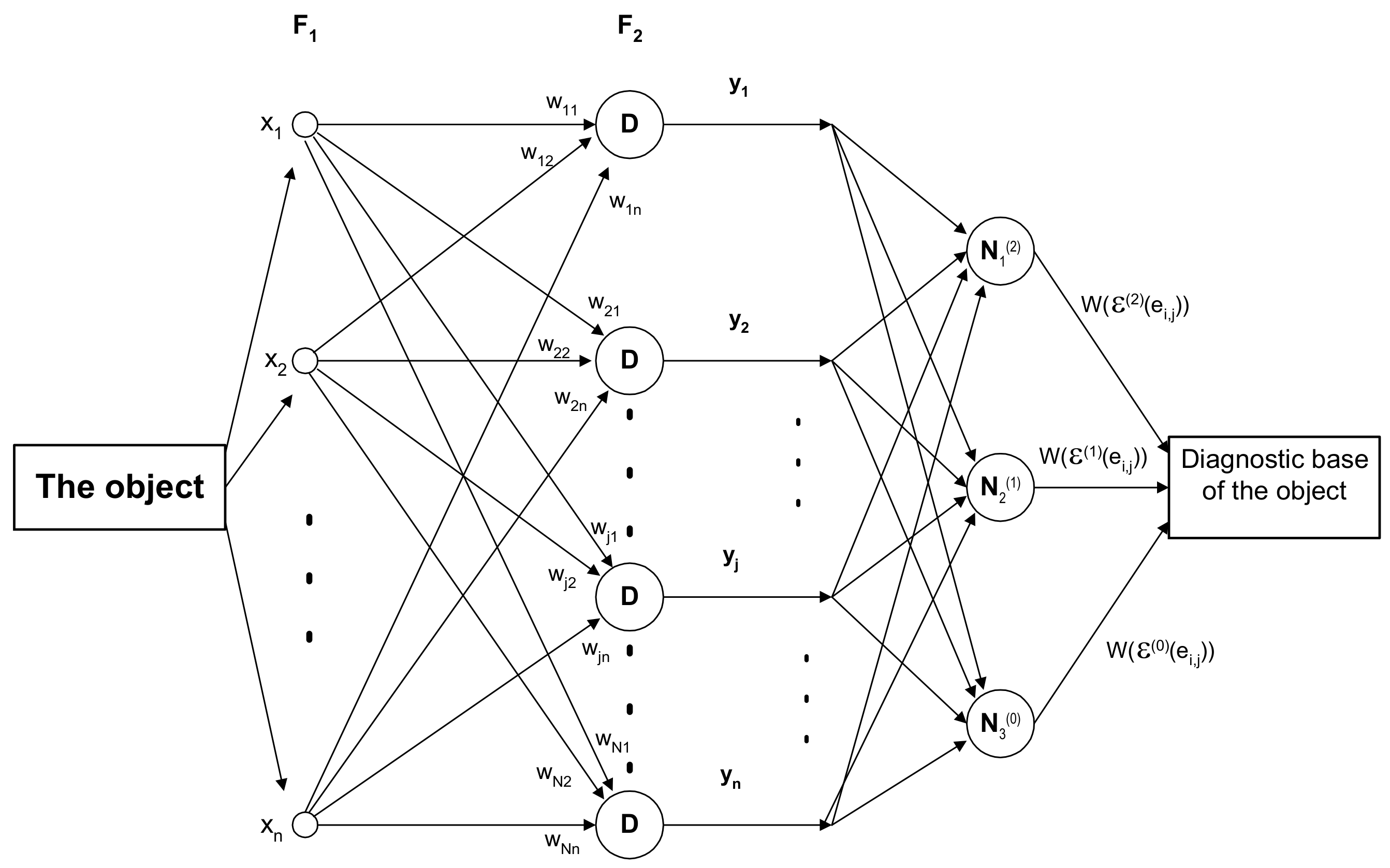
The structure of the artificial neural network used in this article is a proprietary work; it has already been used in publications [10,11]. The network (Figure 2) consists of three layers: F1—input layer, F2—hidden layer and F3—output layer. The neural cells of the network process diagnostic information according to the algorithm (Figure 3 and Figure 4). The entirety of the issues concerning processing of information (Figure 2) by the neurons of the network takes place in the D-dimensional diagnostic space (ω) (Figure 2 and Figure 3) described with the elementary vectors of signals [Xi]. The input signal with the vector form of is given to all the neurons of the input layer of the network. In the cells of the memory of input layer (F1), the standard vectors of signals [X(w)i,j] are recorded. The algorithm of information processing in a diagnostic artificial neural network is presented in Figure 2 and Figure 3.
On this basis, neurons in the input layer calculate the measures of the metrics of the similarity of the compliance of the vector of signal to its vector of the standard in accordance with the following dependence:
Further, the Euclidean measure of the distance metric is calculated; it is presented in the form of the following dependence (3):
In the comparative analysis of diagnostic signals, the special case of the Minkowski measure was applied: when parameter (α = 2) [10]. Then, dependence (3) becomes the Euclidean measure, which is commonly used by the network. Therefore, in the process of input data processing, the transformation is used of input information, whose purpose is to level off too large initial disproportions between the values in the individual dimensions [2,10,11,31,32].
The standardization of data in such a manner that after their conversion the values are within the range [0,1] constitutes a reliable and at the same time quite effective method. The standardization of the metrics of the vectors of signals is realized in accordance with the following dependence:
where the following stand for:
- ΔX(n)i is the standardized vector of the distance metric of jth signal,
- DMi is the standard deviation of ith vector of signal metric,
- X(ei,j) is the diagnostic signal in jth element of ith set,
- X(w)(ei,j) is the model signal for X(ei,j) signal.
On this basis, the calculated dependences (3) and (4) in the input layer of values for all the input vectors are the coefficients of weights , where: i = 1,I; j = 1,J. Weights (υi,j) in the connections of networks have the values from range [0,1].
In the ANN network presented in (Figure 2 and Figure 3), neuron (i) is connected with neuron (j) and sends the signal with value (Xi) with weight coefficient (wi,j) of the activation function presented in the form of the following dependence:
If ith neuron in the network is characterized by the smallest distance of the vector of weights from the input signal, it accepts the value of “1” on its output, and the remaining neurons accept the value of “0”; hence, the name is “the winner takes it all”.
Therefore, for jth neuron with the title of the winner it can be written that the stimulation of this neuron is expressed with the following dependence:
where the following stand for:
- D: the measurement of the similarity of the signal.
- wi,j: weight coefficient
- σi,j: coefficients of weights.
Probabilistic measurements constitute an important category for the definition of the distance function in SBM networks. For this purpose, in the cells (D) of the layer of hidden networks, the probability distribution functions of the normalized metric for the distance of the jth vector of the signal from its standard F(ΔX(n)i) are calculated. In the cells of the memory of the hidden layer, the values are recorded for the normalized distribution of Gauss random variable. When required, the cells in the hidden layer calculate (read) the values of the probability distribution function for the normalized vector of the distance metric of the signal feature for the random variable of metric (ΔX(n)i). The limit value of the probability distribution function for the normalized vector of the distance metric of the signal feature (F(ΔXi)G) is calculated for the random valuable of metric (ΔX(n)i =0), where: (F(ΔXi)G) = 1. The neurons of the hidden layer of the network that realize the calculation of the probability distribution functions for the normalized metrics of distances for the Gaussian-type functions cause the determination of hyper-plane (χ) for the value F(ΔXi)G, which is the standard (limit) value of the probability distribution function for the normalized vector of the distance metric of signal feature. The hyper-plane (χ) constitutes the limit of the decision between the classes of states (Figure 3). This plane is parallel to two points determined with the decision-taking threshold (ς), which lie on a line parallel to hyper-plane (χ).
On the further stage of information processing by the network, the neural cells in the hidden layer of the network calculate the values of weight coefficients (υi,j) on the grounds of the following dependence:
where the following stand for:
- ρi,j: the coefficient of the incompatibility of the input signal vector similarity to its standard vector,
- F(ΔX(n)i): the determined value of the probability distribution function for the normalized distribution concerning the normalized vector of the distance metric of the signal feature,
- F(ΔXi)G: the limit value of the probability distribution function (for the normalized normal distribution) concerning the normalized vector of the distance metric of the signal feature.
Knowing the value of the incompatibility coefficient of the similarity of the input signal vector to its standard vector (ρi,j), on the further stage of work of the network, cells in the hidden layer calculate the compliance coefficient of the similarity of vectors on the grounds of the following dependence:
where the following stand for:
- ωi,j: the compliance coefficient of the similarity of the input signal vector to its standard vector.
On the further stage of the transformation of information in the cells of hidden layer, the value of the output function is calculated on the grounds of the following dependence:
where the following stand for:
- yl: output function,
- ωi,j is the weight coefficient of the network.
3. The Method of the Classification of Elements’ States and the Determination of the State of Objects in the Diagnosing Process in an Intelligent Diagnostic System
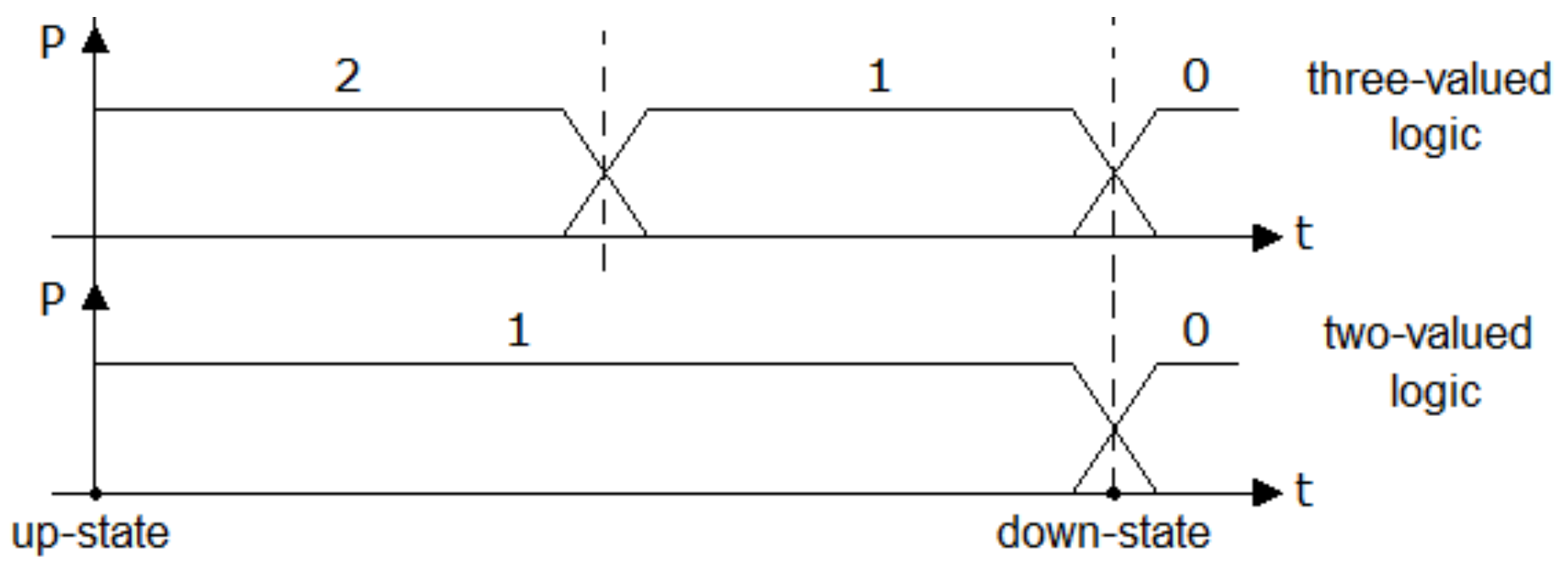
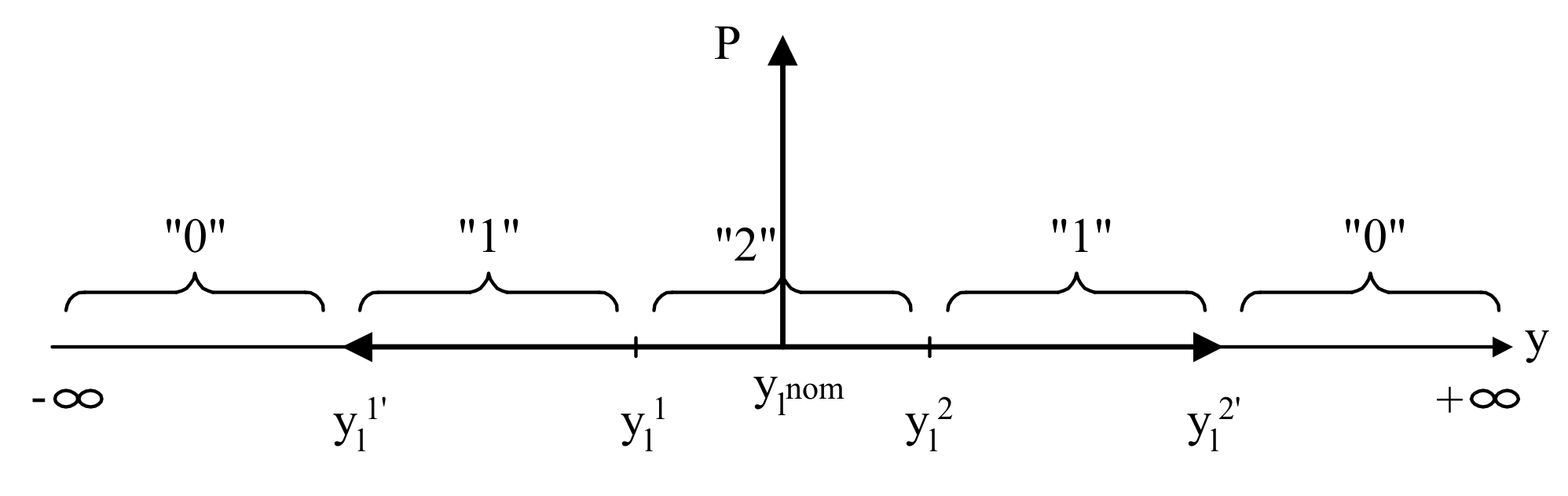
The essence of diagnostics with three-valued state assessment (3VL) is explained in the article. The problem of 3VL diagnostics is developed on the basis of two-valued diagnostics (2VL); its essence is presented in Figure 1. In the 3VL diagnostics, the range of changes in the values 2VL of signals from 2VL logic is accepted, which is assigned the {12VL} state: the serviceability for 2VL. In the three-valued state assessment, an additional inference rule was applied, in which the range of signal changes for the {12VL} serviceability state was divided into two sub-ranges, in which two state values were assigned: {23VL}: the state of serviceability in 3VL logic and {13VL} state: incomplete serviceability state. The state of failure for both applied valences of states is interpreted for the same changes in the values of diagnostic signals, which exceed the possible ranges of their changes; this situation is presented in Figure 4.
As it is presented in the studies [1,2,3,4,5,6,7,10], the purpose of the diagnosis of an object is to identify its state in the values of the valence logic of the assessment of states as accepted by the researcher. Therefore, the decision-making process concerning the classification of states in accordance with the decision threshold accepted in a given network is realized in the output cells of the network. For this purpose, the results obtained in the form of dependence (9) were subject to the process of classification according to the diagram presented in (Figure 5).
On the grounds of the values of the output function determined in the identification process of states, the proper classes of the states of the object in the values of trivalent logic {2, 1, 0} were assigned to them in the classification process of states (Figure 5).
Symbols in Figure 5 represent:
- (yl1, yl2) is the range of insignificant changes of the values of the output function,
- {(yl1′, yl1) and (yl2, yl2′)} is the range of significant changes of the output function values,
- {(−∞, yl1′) and (yl2′, +∞)} is the range of impermissible changes of the output function values.
The accepted classes of states are defined in the following way:
- State of fitness: this constitutes the fitness of an element to which the state marked with the value “2” was assigned. In this state, changes of the output function (yl) values are within the following range:where the following stand for: Rw1 is the 1st rule of diagnostic inference, is the range of irrelevant changes for the values of the features of signal, is a symbol of comparison, {3} is the operable condition.
- State of incomplete serviceability: this constitutes an incomplete serviceability of an element, which the state marked with the value “1” was assigned to. In this state, a change in the output function (yl) value is to be within the following range:where the following stand for: Rw2 is the 2nd rule of diagnostic inference, is the range of changes for the relevant values of the features of signal, is a symbol of comparison, {2} is the incomplete operable condition.
- State of unfitness: this constitutes an unfitness of a basic element, which was assigned with the state marked with value “0”. In this state, the change of the output function yl values is outside the ranges of permissible changes (defined with the decision threshold β of the network (Figure 5):where the following stand for: Rw3 is the 3rd rule of diagnostic inference, ) is the inadmissible range for the values of the features of signal, is a symbol of comparison, {0} is the condition of inoperability.
4. Research and Results of the Determination of a Diagnostic Information of Low-Power Solar Plant Devices (L-PSPD) with the Use of an Artificial Neural Network
In the diagnostics of low-power solar plant devices, the proprietary intelligent DIAG 2 system operating on the basis of an artificial neural network of the RBF type was used. The descriptive part of the article presents the algorithm of the diagnostic method implemented in the DIAG 2 intelligent diagnostic system. The diagnostic method presented in the DIAG 2 system utilizes the method known in the literature [10,11] used for comparing diagnostic signals with the appropriate standard diagnostic signal vector assigned to them, cf. Relationship (1). The form of diagnostic information developed in the DIAG 2 system is expressed in the three-valued state evaluation {2, 1, 0}. The result of this diagnostic information from the DIAG 2 program is summarized in a tabular form: “Table states of objects”. In order to carry out the tests accepted in a small solar power plant system, an experimental stand was made, as shown in Figure 6.
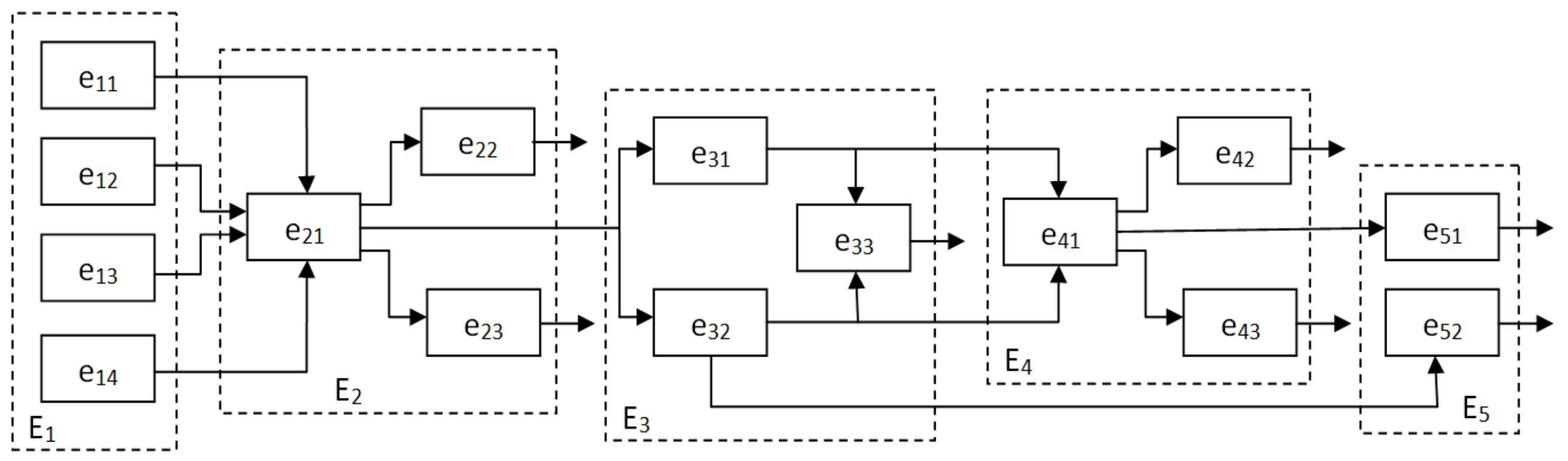
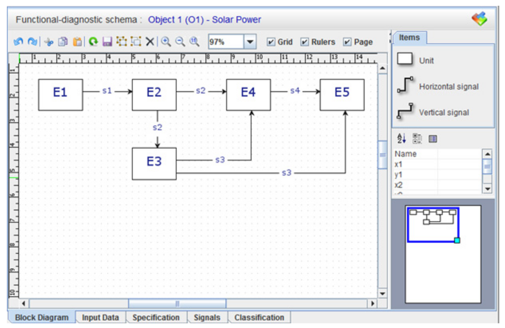
The use of the DIAG 2 diagnostic system to carry out diagnostic tests requires that a diagnostic study of the object examined be performed beforehand. The reader will find examples and the manner of implementing this diagnostic intention in the following paper: [10]. For the purposes of the research, a functional and diagnostic analysis of devices in the low-power solar plant devices was carried out. The result of this analysis is a designated set of ith functional units {Ei}. At the next stage of the analysis, the set of jth basic elements was determined in each ith group {ei, j}. The functional units of the object are presented in the DIAG 2 diagnostic system, and they are marked as “units”, while the basic elements are marked as jth “elements”. The subassemblies in the ith assemblies of the facility are considered third-level elements: “Modules” acting as “intermediate elements”. The modules enable bidirectional transformation of the hierarchical form of an object into a matrix internal structure presented in Figure 7 and Figure 8.
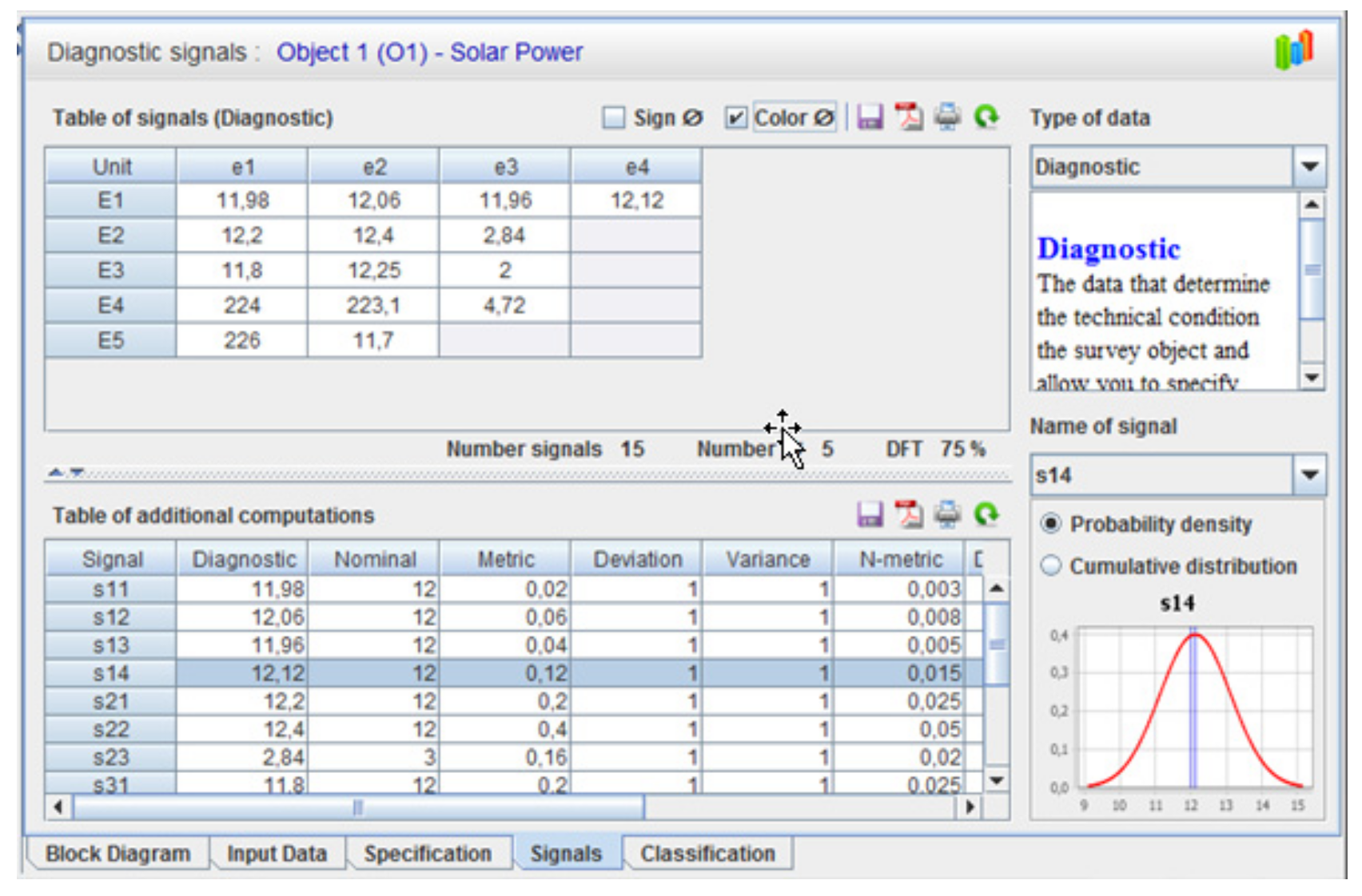
Starting the DIAG 2 diagnostic system requires the attachment (saving in the program memory) of the developed diagnostic measurement knowledge base. The measurement base consists of diagnostic signals {X(ei,j)} appearing at the output of the jth object elements and the associated diagnostic standard signals {Xw(ei,j)}. The set of the measurement base developed for the DIAG program is presented in Figure 8.
The diagnostic state of the object examined in the DIAG system is determined on the basis of an examination and analysis as well as comparing the image of the set of output diagnostic signals with their image of the reference signal (nominal) (Figure 9) [2,3,4,5,6,7,8,9,10,11].
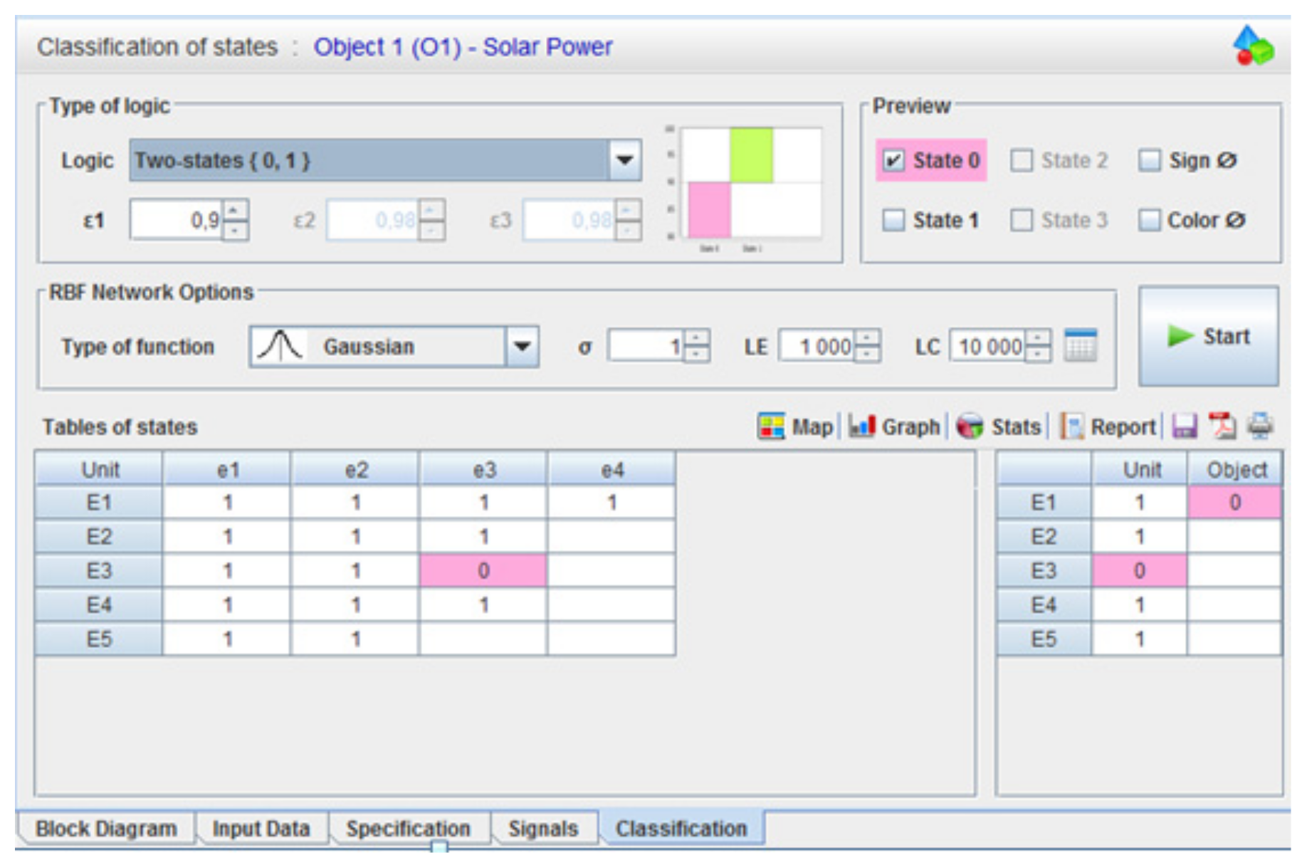
The DIAG diagnostic system develops the final form of diagnostic information in one of two possible assessments of the state of the object with 2- or 3-valued logic. The final form of diagnostic information about the states of the object examined is compiled in the state table for 2VL-two-valued state evaluation, where the determined states are determined by the value from the {1, 0} set (Figure 10).
The diagnostic result in the bivalent assessment of 2VL states of low-power solar power plant equipment is shown in Figure 10. The figure shows that the states of the j basic elements included in the subset {e1,1; e1,2; e1,3; e1,4; e2,1; e2,2; e2,3; e3,1; e3,2; e4,1; e4,2; e4,3; e5,1; e5,2} possess the state “1”—the state of fitness. Only one basic element of the object marked {e3,3} has the state “0”—the state of unfitness.
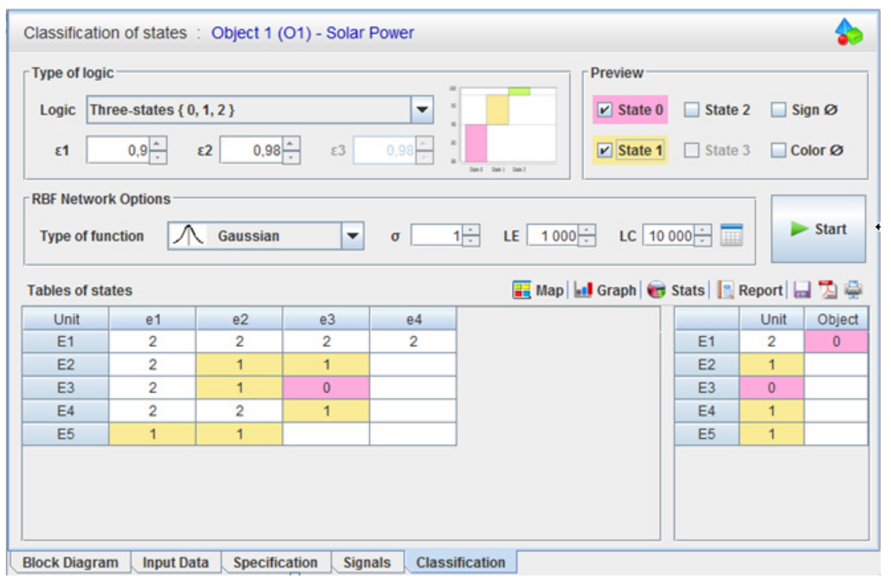
The final form of the diagnostic information concerning the states of the object examined is compiled in the state table for 3VL—three-valued state evaluation, where the determined states are determined by the value from the {2, 1, 0} set (Figure 11).
The result of the diagnostics of low-power solar plant devices in the three-valued 3VL state assessment in Figure 11 shows that the basic elements of the subset {e1,1; e1,2; e1,3; e1,4; e2,1; e3,1; e4,1; e4,2} possess the state “2”—the state of fitness. However, the basic elements of the object from the set {e2,2; e2,3; e3,2; e4,3; e5,1; e5,2} possess the “1” state-incomplete condition. As in the case of 2VL diagnostics, in the 3VL diagnostics only one basic element marked {e3,3} has the state “0”—the state of unfitness.
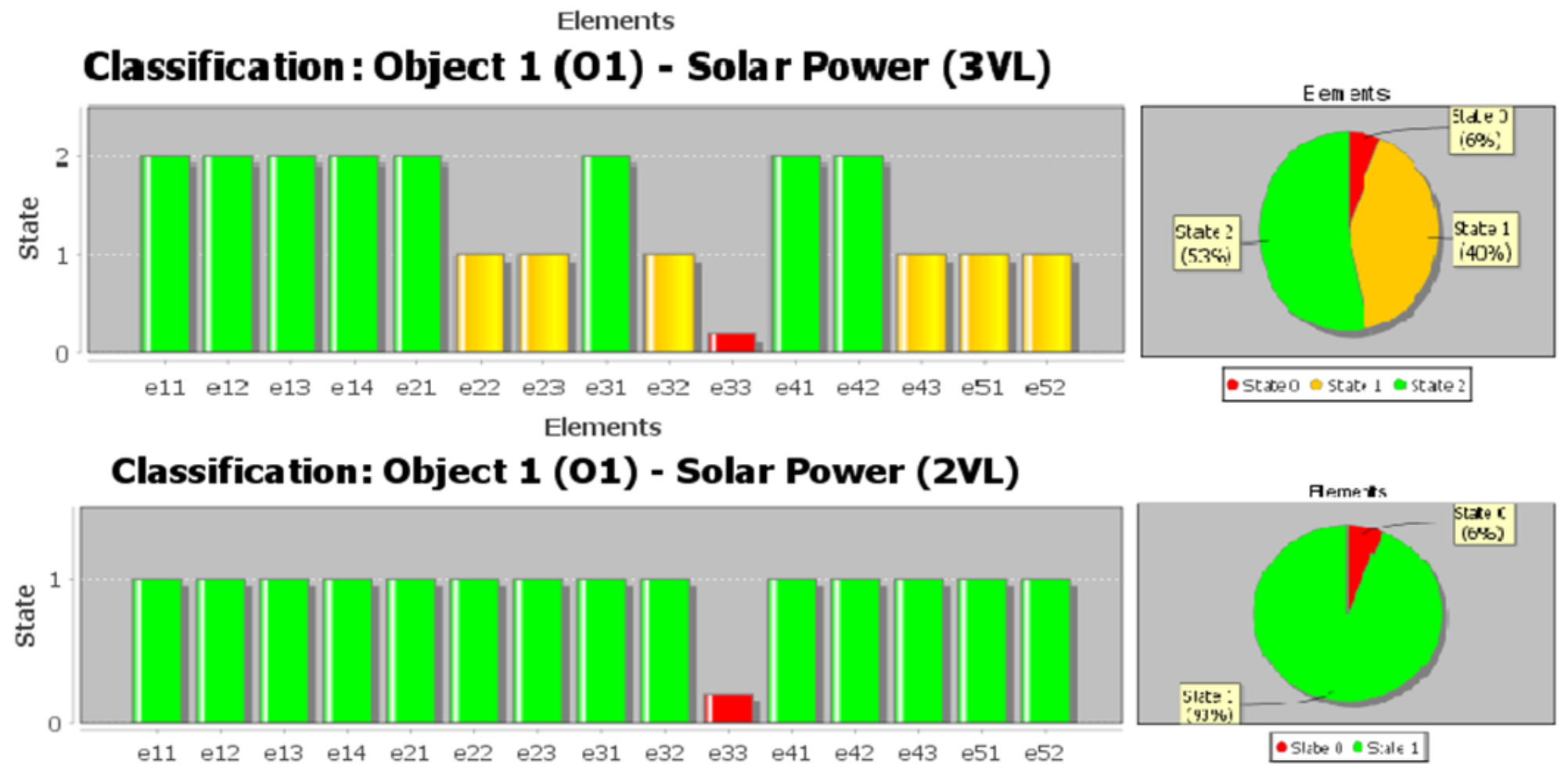
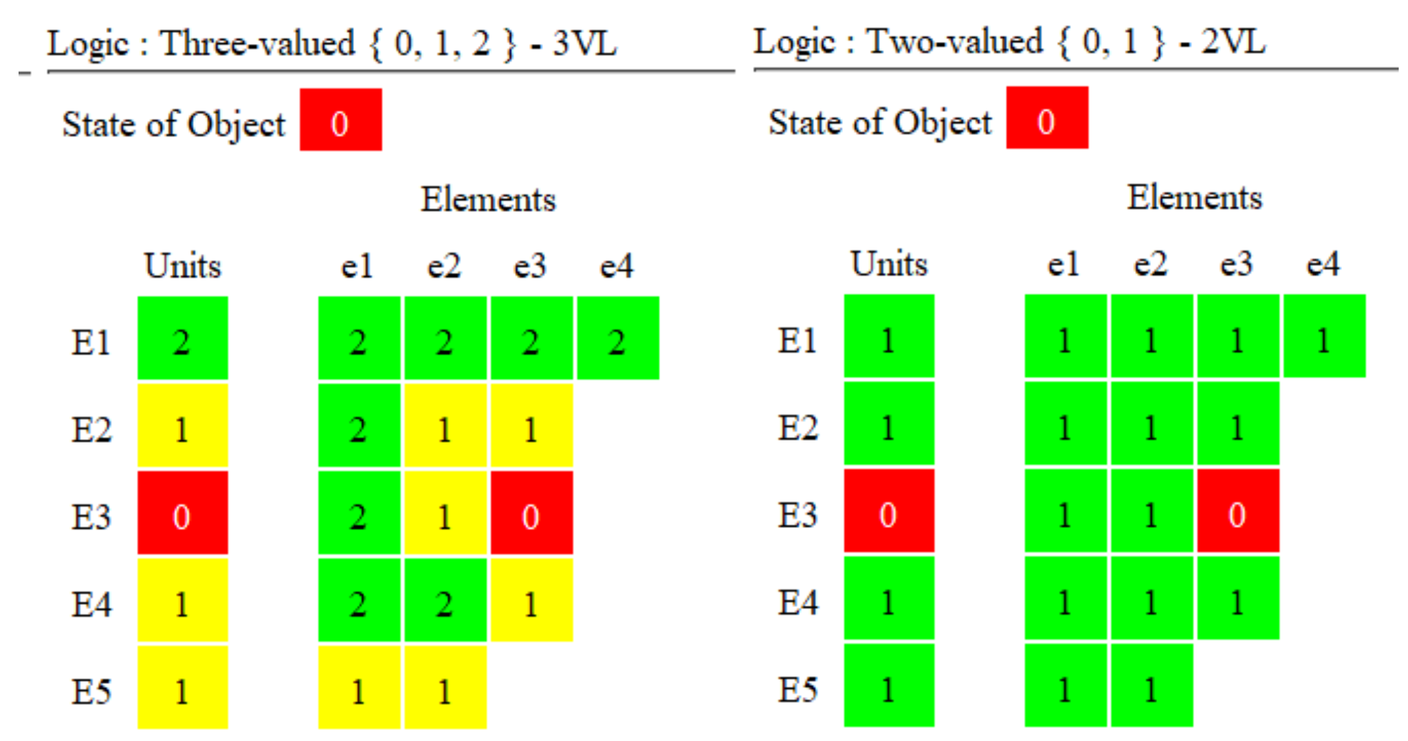
Figure 12 and Figure 13 show the screens of collective diagnostic information developed in the DIAG 2 program for diagnosis in 3-valued logic 3VL and diagnosis expressed in 2-valued logic 2VL.
Based on the diagnostic information in Figure 12 and Figure 13, it can be concluded that for low-power solar plant devices, for both of the state assessment logics used in the valence test the DIAG 2 system recognized one basic element marked {e3,3} with the status “0”-state of unfitness. On this basis, it can be concluded that the diagnostic rules presented as dependencies (2 and 3) developed in the system DIAG 2 are correct. The analysis of Figure 12 shows that the reasoning and informationality of the diagnoses developed in the DIAG system in 3-valued logic (3VL) is more informative because the DIAG 2 system additionally recognizes the {1} state—the state of incomplete compliance. Therefore, it can be stated, which is already known, e.g., from theoretical considerations presented in the literature [2,3,4,5,6,7,8,9,10,11,12,13], that in 3-valued logic the determined state “1”—incomplete condition, makes this 3VL logic more informative than 2VL 2-valued logic.
Chapter Four presents the core of the issue of low-power solar plant devices. The diagnosis process of any technical object is a complicated technical and organizational operation. The elements of that operation include the following: 1—a functional and diagnostic analysis of an object under examination, 2—elaborating a diagnostic system (computer program), 3—determining a measurement data base of an object. A prerequisite for diagnosing an object is to carry out a functional and diagnostic analysis on the object under examination. “What is the basis of this analysis” is an accepted method of division of the object’s internal structure, e.g., three- or four-level division. Due to that, a set of basic elements of the object is determined, and those elements form the object’s structure; thus, their diagnostic state determines (implicates) the states of individual units (functional systems). The states recognized of the functional systems of an object determine the state of the object under examination.
The use of an artificial neural network on the basis of which the DIAG 2 diagnostic system works is an effective research and analytical tool, especially for such objects tested as low-power solar plant equipment. The basis for the implementation of diagnostics is an effective measurement system that will develop a measurement knowledge base. Such a designated database of measurement knowledge (a subset of diagnostic signal values) must be supplemented with a subset of standard diagnostic signal values designated for this database (Figure 9).
In order to diagnose low-power solar plant devices, a method of analyzing similar images, being presented in the paper, was used. Based on that method, an artificial neural network algorithm and a computer program DIAG 2 were elaborated. The paper presents a full approach to diagnosing technical objects and installations. This work model presented by a diagnostician is essential to determine the state of the object under examination. For that purpose, an internal structure of the object under examination was divided according to the following three-level scheme: Object-Functional System-Basic Element or module of the object. This resulted in a set of basic elements and a set of diagnostic signals, which are shown in charts.
5. Discussion
The purpose of this article, as presented in the introduction, is to prove the truth of the thesis: diagnoses in logic (3VL) are more informative (contain more information) than diagnoses expressed in logic (2VL). The research results obtained and their analysis, which was carried out on the basis of the results presented in Figure 12 and Figure 13, confirm the research thesis presented in this way. Theoretically, the literature shows that the diagnostic information efficiency in logic (3VL) is greater than (2VL). In the papers on the organization of the process of refurbishing technical objects, the author demonstrated that the diagnoses in logic (3VL) are more informative. In this manner, a strategy for organizing the process of renewing complex technical facilities such as solar power plants was developed. The results of papers concerning this subject are presented in the literature. In this article, the authors attempted a practical verification of the sis presented. The research presents a high standard of organization of the research process by meeting the following conditions:
- tests were conducted for each of the assessed logics (3VL and 2VL) on the same test object;
- the same research tool was used in the research, i.e., the DIAG 2 computer program;
- the research was conducted on the same input data (diagnostic signals).
Organized research concerning the informational value of diagnoses for a solar power plant is objective and independent. Hence, the obtained results were considered true. The practical assessment of the results in terms of the informational value of the diagnoses examined (3VL and 2VL) is as follows.
- In each of the valences examined of diagnoses (3VL and 2VL), only one and the same element of the object {e3,3} was designated, which possesses the state “0”: the state of unfitness. This shows that the DIAG 2 system correctly recognizes the states, i.e., the artificial neural network classifies the states of the elements well;
- A practical criterion was adopted in the assessment of the informational value of the diagnoses examined (3VL and 2VL). This criterion is based on the fact that the evaluation of the informational value of diagnoses in a given evaluation logic is determined on the basis of the number of additional states occurring in a given logic, apart from the states of fitness and unfitness, because they are common in these evaluations;
- In logic (3VL), there is a state of incomplete fitness, which is absent in logic (2VL); hence, the number of states, and more precisely (%) of all the states of elements with the state “1” recognized, will directly indicate the assessment of informational value of this diagnosis in relation to evaluation (2VL);
- In the examination of the logic (3VL), state “1” was recognized for elements from the subset {e2,2; e2.3; e3.2; e4.3; e5.1; e5.2}. This subset of states constitutes 40% of all the states examined of the object’s elements. On this basis, the informational value of the diagnosis (3VL) in relation to the diagnosis (2VL) was determined;
- On the basis of conclusion (4), the final conclusion of the study was developed, namely that the information efficiency of the diagnosis (3VL) is 40% greater than that of the diagnosis (2VL).
6. Conclusions
Based on the results obtained from the research, it appears that the diagnoses presented in 3-valued logic in terms of informationality are larger (richer) than diagnoses expressed in 2-valued logic. The percentage share of the j-th elements having an incomplete condition {1} (Figure 12) in the structure of the object tested is 40%. Therefore, on this basis, the percentage information yield of three-valued (3VL) diagnostics was calculated; in relation to the two-valued diagnostics (2VL) it is 40% higher.
The use of an artificial neural network on the basis of which the DIAG 2 diagnostic system works is an effective research and analytical tool, especially for such objects tested as of low-power solar plant equipment. The basis for the implementation of diagnostics is an effective measurement system that will develop a measurement knowledge base. Such a designated database of measurement knowledge (a subset of diagnostic signal values) must be supplemented with a subset of standard diagnostic signal values designated for this database (Figure 9).
Diagnosing technical objects in 3-valued logic makes this diagnostics more useful due to the need to use the information developed in the DIAG system for the process of organizing technical maintenance (repair and renewal process). Interpreting (recognizing) the incomplete condition of the facility enables the use of an optimal strategy for organizing its technical maintenance (renewal) in the facility tested, based on an assessment of the reliability condition of the facility’s components. Diagnostics with a three-valued state assessment in complex technical objects is anticipatory. It means that the first repair (renewal) of the jth elements possess the state “1”. This problem is particularly important for the use and operation of those complex technical facilities that are characterized by short downtime.
Author Contributions
Conceptualization, resources, methodology, software, validation, S.D. and M.W.; formal analysis, investigation, data curation, J.V. and D.B.; writing—original draft preparation, writing—review and editing, visualization, J.P. and M.S.; supervision, project administration, funding acquisition, R.D. All authors have read and agreed to the published version of the manuscript.
Funding
This research was funded by Faculty of Electronic and informatics, Technical University of Koszalin, 2 Sniadeckich St., 75-620 Koszalin, Poland.
Institutional Review Board Statement
Not applicable.
Informed Consent Statement
Not applicable.
Data Availability Statement
The data presented in this article are available on request of the corresponding author.
Conflicts of Interest
The authors declare no conflict of interest.
Symbols and Acronyms
| E1 | photovoltaic system |
| E2 | voltage regulator (driver) system |
| E3 | electric energy storage system |
| E4 | DC/AC converter |
| E5 | receiving system |
| X(ei,j) | diagnostic signal in jth element of ith set |
| X(w)(ei,j) | model signal for X(ei,j) signal |
| FC max | max. value of the function of the use of the object |
| ΔX(n)i | standardized vector of the distance metric of jth signal |
| DMi | standard deviation of ith vector of signal metric |
| W(ε(ei,j)) | valued of state assessment logics for jth element within ith module (from the set of the accepted three-value logic of states’ assessment) |
| {ME(ei,j)} | specialist knowledge base (a set of maintenance information of the object) |
| DM(Xi, X(w)i α) | standard deviation of the vector the signal metric, (α = 2) |
| Xn | the nth diagnostic signal in jth element of ith set |
| wi,n | weight coefficient |
| σi,j | coefficients of weights |
| w(ε(0)(ei,j))i,j | compliance coefficient of the similarity of the input signal vector to its standard vector for the diagnostic signal in jth element of ith set |
| (4VL) | four-valued state rating |
| DIAG | Invented name of Intelligent Diagnostic System |
| ANN | artificial neural network |
| RBF | Radial Basis Function type of ANN |
| SBM | similarity-based methods is type of ANN |
| {3} | set of fitness states |
| {2} | set of incomplete states |
| {1} | set of critical fitness states |
| {0} | set of states of unfitness |
| (3VL) | three-valued state assessment |
| {2} | set of states of fitness |
| {1} | set of incomplete states |
| {0} | set of states of unfitness |
| (2VL) | two-valued state assessment |
| {1} | set of states of fitness |
| {0} | set of states of unfitness |
References
- Hojjat, A.; Hung, S.L. Machine Learning, Neural Networks, Genetic Algorithms and Fuzzy Systems; John Wiley & Sons, Inc.: Hoboken, NJ, USA, 1995; p. 398. [Google Scholar]
- Madan, M.; Gupta, M.; Liang, J.; Homma, N. Static and Dynamic Neural Networks, from Fundamentals to Advanced Theory; John Wiley & Sons, Inc.: Hoboken, NJ, USA, 2003; p. 718. [Google Scholar]
- Zurada, I.M. Introduction to Artificial Neural Systems; West: London, UK, 2007. [Google Scholar]
- Tang, L.; Liu, J.; Rong, A.; Yang, Z. Modeling and genetic algorithm solution for the slab stack shuffling problem when implementing steel rolling schedules. Int. J. Prod. Res. 2002, 40, 272–276. [Google Scholar] [CrossRef]
- Wiliams, J.M.; Zipser, D. A learning Algorithm for Continually Running Fully Recurrent Neural Networks. Neural Comput. Appl. 1989, 1, 270–280. [Google Scholar] [CrossRef]
- Linz, P.; Wang, R. Exploring Numerical Methods: An Introduction to Scientific Computing Using Matlab; University of California: Davis, CA, USA, 2003. [Google Scholar]
- Linz, P. An Introduction to Formal Languages and Automata; University of California: Davis, CA, USA, 2002. [Google Scholar]
- Buchannan, B.; Shortliffe, E. Rule—Based Expert Systems; Addison—Wesley Publishing Company: London, UK, 1985; p. 387. [Google Scholar]
- Waterman, D. A Guide to Export Systems; Addison—Wesley Publishing Company: London, UK, 1986; p. 545. [Google Scholar]
- Duer, S. Artificial neural network in the control process of object’s states basis for organization of a servicing system of a technical objects. Neural Comput. Appl. 2012, 21, 153–160. [Google Scholar] [CrossRef]
- Duer, S. Applications of an artificial intelligence for servicing of a technical object. Neural Comput. Appl. 2012, 22, 955–968. [Google Scholar] [CrossRef]
- Birolini, A. Reliability Engineering Theory and Practice; Springer: New York, NY, USA, 1999; p. 221. [Google Scholar]
- Ushakov, I.A. Handbook of Reliability Engineering; John Wiley & Sons: New York, NY, USA, 1994. [Google Scholar]
- Barlow, R.E.; Proschan, F. Mathematical Theory of Reliability; John Wiley & Sons: New York, NY, USA, 1995; p. 335. [Google Scholar]
- Dhillon, B.S. Applied Reliability and Quality, Fundamentals, Methods and Procedures; Springer: London, UK, 2006; p. 186. [Google Scholar]
- Kacalak, W.; Majewski, M. Effective Handwriting Recognition System Using Geometrical Character Analysis Algorithms; Lecture Notes in Computer Science 7666, Part IV; Springer: Berlin/Heidelberg, Germany, 2012; pp. 248–255. [Google Scholar]
- Kacalak, W.; Majewski, M. New Intelligent Interactive Automated Systems for Design of Machine Elements and Assemblies; Lecture Notes in Computer Science 7666, Part IV; Springer: Berlin/Heidelberg, Germany, 2012; pp. 115–122. [Google Scholar]
- Lipinski, D.; Majewski, M. System for Monitoring and Optimization of Micro- and Nano-Machining Processes Using Intelligent Voice and Visual Communication; Lecture Notes in Computer Science; Springer: Berlin/Heidelberg, Germany, 2013; Volume 8206, pp. 16–23. [Google Scholar]
- Nakagawa, T. Maintenance Theory of Reliability; Springer: London, UK, 2005; p. 264. [Google Scholar]
- Nakagawa, T.; Ito, K. Optimal inspection policies for a storage system with degradation at periodic tests. Math. Comput. Model. 2000, 31, 191–195. [Google Scholar]
- Rosiński, A. Design of the electronic protection systems with utilization of the method of analysis of reliability structures. In Proceedings of the Nineteenth International Conference on Systems Engineering (ICSEng 2008), Las Vegas, NV, USA, 19–21 August 2018. [Google Scholar]
- Rosiński, A. Reliability analysis of the electronic protection systems with mixed—Three branches reliability structure. In Reliability, Risk and Safety. Theory and Applications; Bris, R., Guedes Soares, C., Martorell, S., Eds.; CRC Press/Balkema: London, UK; RC Press—Taylor & Francis Group: Boca Raton, FL, USA, 2019; Volume 3. [Google Scholar]
- Stawowy, M.; Olchowik, W.; Rosiński, A.; Dąbrowski, T. The Analysis and Modelling of the Quality of Information Acquired from Weather Station Sensors. Remote Sens. 2021, 13, 693. [Google Scholar] [CrossRef]
- Stawowy, M.; Rosiński, A.; Paś, J.; Klimczak, T. Method of Estimating Uncertainty as a Way to Evaluate Continuity Quality of Power Supply in Hospital Devices. Energies 2021, 14, 486. [Google Scholar] [CrossRef]
- Palkova, Z.; Okenka, I. Programming; Slovak University of Agriculture in Nitra: Nitra, Slovakia, 2007; p. 203. [Google Scholar]
- Pokoradi, L. Logical Tree of Mathematical Modeling. Theory Appl. Math. Comput. Sci. 2015, 5, 20–28. [Google Scholar]
- Pokoradi, L. Failure Probability Analysis of Bridge Structure Systems. In Proceedings of the 10th Jubilee IEEE International Symposium on Applied Computational Intelligence and Informatics, Timişoara, Romania, 21–23 May 2015. [Google Scholar]
- Zajkowski, K. The method of solution of equations with coefficients that contain measurement errors, using artificial neural network. Neural Comput. Appl. 2014, 24, 431–439. [Google Scholar] [CrossRef] [PubMed] [Green Version]
- Kobayashi, S.; Nakamura, K. Knowledge compilation and refinement for fault diagnosis. IEEE Expert 1991, 6, 39–46. [Google Scholar] [CrossRef]
- Teramoto, T.; Nakagawa, T.; Motoori, M. Optimal inspection policy for a parallel redundant system. Microelectron. Reliab. 1990, 30, 151–155. [Google Scholar] [CrossRef]
- Duer, S. Examination of the reliability of a technical object after its regeneration in a maintenance system with an artificial neural network. Neural Comput. Appl. 2012, 21, 523–534. [Google Scholar] [CrossRef]
- Duer, S.; Bernatowicz, D.; Wrzesień, P.; Duer, R. The diagnostic system with an artificial neural network for identifying states in multi-valued logic of a device wind power. In Communications in Computer and Information Science; Springer: Poznan, Poland, 2018; Volume 928, pp. 442–454. [Google Scholar]
- Duer, S. Assessment of the Operation Process of Wind Power Plant’s Equipment with the Use of an Artificial Neural Network. Energies 2020, 13, 2437. [Google Scholar] [CrossRef]
- Duer, S.; Zajkowski, K.; Harničárová, M.; Charun, H.; Bernatowicz, D. Examination of Multivalent Diagnoses Developed by a Diagnostic Program with an Artificial Neural Network for Devices in the Electric Hybrid Power Supply System “House on Water”. Energies 2021, 14, 2153. [Google Scholar] [CrossRef]
- Hwang, H.R.; Kim, B.S.; Cho, T.H.; Lee, I.S. Implementation of a Fault Diagnosis System Using Neural Networks for Solar Panel. Int. J. Control Autom. Syst. 2019, 17, 1050–1058. [Google Scholar] [CrossRef]
- Ganeshprabu, B.; Geethanjali, M. Dynamic Monitoring and Optimization of Fault Diagnosis of Photo Voltaic Solar Power System Using ANN and Memetic Algorithm. Circuits Syst. 2016, 7, 3531–3540. [Google Scholar] [CrossRef] [Green Version]
- Jiang, L.L.; Maskell, D.L. Automatic fault detection and diagnosis for photovoltaic systems using combined artificial neural network and analytical based methods. In Proceedings of the 2015 International Joint Conference on Neural Networks (IJCNN), Killarney, Ireland, 12–16 July 2015; pp. 1–8. [Google Scholar] [CrossRef]
- Duer, S.; Wrzesień, P.; Duer, R.; Bernatowicz, D. Diagnostics of low-capacity solar power station equipment with 2- and 3-valued logic. Bull. Mil. Univ. Technol. 2018, lXVII. [Google Scholar] [CrossRef]
- Xiao, W.; Nazario, G.; Wu, H.; Zhang, H.; Cheng, F. A neural network based computational model to predict the output power of different types of photovoltaic cells. PLoS ONE 2017, 12, e0184561. [Google Scholar] [CrossRef] [Green Version]
- Huang, J.; Wai, R.; Gao, W. Newly-Designed Fault Diagnostic Method for Solar Photovoltaic Generation System Based on IV-Curve Measurement. IEEE Access 2019, 7, 70919–70932. [Google Scholar] [CrossRef]
Figure 1.
Diagram of an intelligent effective diagnosing system of a complex technical object.

Figure 2.
Structure of an artificial neural network in the DIAG system.

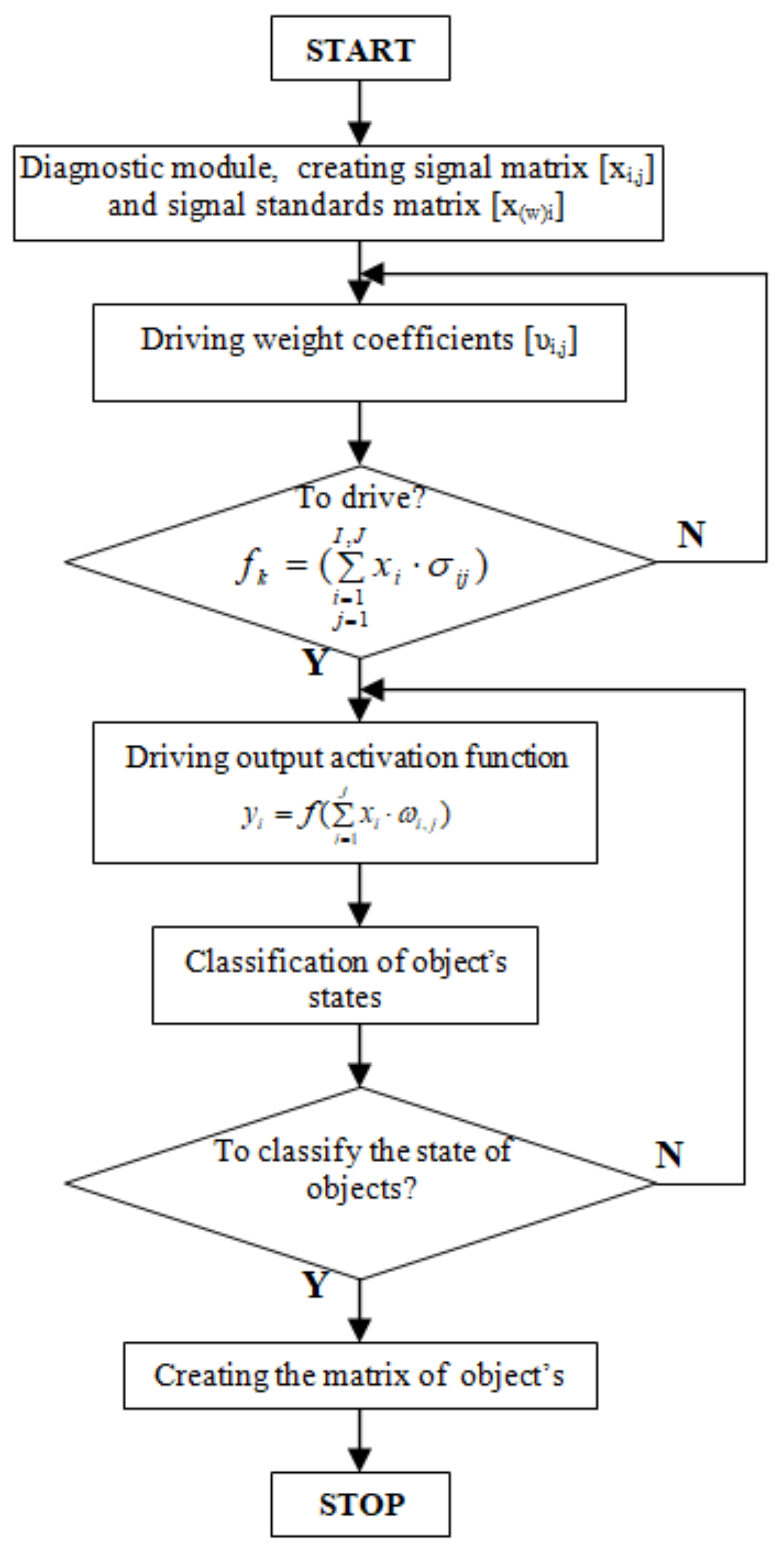
Figure 3.
The algorithm of diagnostic program DIAG.

Figure 4.
Diagram of the bases of diagnosing based on change to the k-th property of the diagnostic signal, for concluding in three-valued logic (3VL).
Figure 4.
Diagram of the bases of diagnosing based on change to the k-th property of the diagnostic signal, for concluding in three-valued logic (3VL).

Figure 5.
Ranges of the changes of the output function values.

Figure 6.
Diagram of functional and diagnostic structure of low-power solar plant devices.

Figure 7.
Result form of DIAG 2 program for “Structure” module.

Figure 8.
Technical object classification panel for “Signal values” module.

Figure 9.
Program screen DIAG 2 in the form of “Diagnostic signals table”.

Figure 10.
The result form of the DIAG 2 program “Table of states of L-PSPD” for 2VL.

Figure 11.
The resulting form of the DIAG 2 program “Table of states of L-PSPD” for 3VL.

Figure 12.
Screen of comparative analysis of the state assessment of L-PSPD in the DIAG 2 program.

Figure 13.
Screen of comparative analysis of the state assessment of L-PSPD in the DIAG 2 program.


Table 1.
Table of the states of the object’s elements.
| Number of the Assembly | Vector of the States of Basic Elements in the Structure of the Object {ei,j} | ||||
|---|---|---|---|---|---|
| ε (e1,1) | … | ε (ei,j) | … | ε (ei,J) | |
| E1 | W (ε (e1,1)) | … | W(ε (e1,j)) | … | W (ε (e1,J)) |
| … | … | ||||
| Ei | W (ε (ei,1)) | … | W(ε (ei,j)) | … | ∅ |
| … | … | ||||
| EI | W (ε (eI,1)) | … | W(ε (eI,j)) | … | W(ε (eI,J)) |
where the following stand for: W (ε (ei,j)) is the value of the state of jth element in ith unit (from the set of the accepted trivalent logic of the assessment of states—{2, 1, 0}), ∅ is the element which complements the dimension of the table, Ei is the ith functional assembly of the object.
Publisher’s Note: MDPI stays neutral with regard to jurisdictional claims in published maps and institutional affiliations. |
© 2021 by the authors. Licensee MDPI, Basel, Switzerland. This article is an open access article distributed under the terms and conditions of the Creative Commons Attribution (CC BY) license (https://creativecommons.org/licenses/by/4.0/).
Share and Cite
MDPI and ACS Style
Duer, S.; Valicek, J.; Paś, J.; Stawowy, M.; Bernatowicz, D.; Duer, R.; Walczak, M. Neural Networks in the Diagnostics Process of Low-Power Solar Plant Devices. Energies 2021, 14, 2719. https://doi.org/10.3390/en14092719
AMA Style
Duer S, Valicek J, Paś J, Stawowy M, Bernatowicz D, Duer R, Walczak M. Neural Networks in the Diagnostics Process of Low-Power Solar Plant Devices. Energies. 2021; 14(9):2719. https://doi.org/10.3390/en14092719
Chicago/Turabian StyleDuer, Stanisław, Jan Valicek, Jacek Paś, Marek Stawowy, Dariusz Bernatowicz, Radosław Duer, and Marcin Walczak. 2021. "Neural Networks in the Diagnostics Process of Low-Power Solar Plant Devices" Energies 14, no. 9: 2719. https://doi.org/10.3390/en14092719
Note that from the first issue of 2016, this journal uses article numbers instead of page numbers. See further details here.