
Component-in-the-Loop Testing of Automotive Powertrains Featuring All-Wheel-Drive
by
 ,
,
Ilya Kulikov
1,*, 
Sergey Korkin
1,
Andrey Kozlov
1,
Alexey Terenchenko
1,
Kirill Karpukhin
1 and
Ulugbek Azimov
2
1
National Research Center “NAMI”, 125438 Moscow, Russia
2
Faculty of Engineering and Environment, Northumbria University, Newcastle upon Tyne NE1 8ST, UK
*
Author to whom correspondence should be addressed.
Energies 2021, 14(7), 2017; https://doi.org/10.3390/en14072017
Submission received: 26 February 2021
/
Revised: 30 March 2021
/
Accepted: 31 March 2021
/
Published: 6 April 2021
(This article belongs to the Section E: Electric Vehicles)
Abstract
:The article is dedicated to the methodology of designing component-in-the-loop (CiL) testing systems for automotive powertrains featuring several drivelines, including variants with individually driven axles or wheels. The methodical part begins with descriptions of operating and control loops of CiL systems having various simulating functionality—from a “lumped” vehicle for driving cycle tests to vehicles with independently rotating drivelines for simulating dynamic maneuvers. The sequel contains an analysis that eliminates a lack of clarity observed in the existing literature regarding the principles of building a “virtual inertia” and synchronization of loading regimes between individual drivelines of the tested powertrain. In addition, a contribution to the CiL methodology is offered by analyzing the options of simulating tire slip taking into account a limited accuracy of measurement equipment and a limited performance of actuating devices. The methodical part concludes with two examples of mathematical models that can be employed in CiL systems to simulate vehicle dynamics. The first one describes linear motion of a “lumped” vehicle, while the second one simulates vehicle’s trajectory motion taking into account tire slip in both the longitudinal and lateral directions. The practical part of the article presents a case study showing an implementation of the CiL design principles in a laboratory testing facility intended for an all-wheel-drive hybrid powertrain of a heavy-duty vehicle. The CiL system description is followed by the test results simulating the hybrid powertrain operation in a driving cycle and in trajectory maneuvering. The results prove the validity of the proposed methodical principles, as well as their suitability for practical implementations.
1. Introduction
Automotive powertrains, especially those with multiple driving axles or individually driven wheels, besides propelling the vehicle, can deliver several functions including control of traction and braking forces [1,2,3] and the yaw stability control also called torque vectoring [1,4,5]. When elaborating these functions using physical experiments, the powertrain or its components should be tested in regimes corresponding to vehicle driving that ranges from linear motion to intensive trajectory maneuvering. Among the existing experimental methods suitable for that task, vehicle road tests are able to provide the widest range of possible driving modes and external conditions. Moreover, tests of that type produce results being closest to real-world driving. However, they have a number of limitations, which can be divided into two kinds. The first one implies limitations imposed by season and weather conditions including possible instability of physical properties of the road surface (e.g., instability of snow and ice under the direct sun). This may entail difficulties in ensuring repeatability of tests. The second kind relates to measurement constraints especially when it comes to the operating parameters of the powertrain that have to be measured in difficult-to-access places.
Thorough and comprehensive physical tests of powertrains can be performed in a laboratory using test benches. This approach provides a convenient access to the powertrain components allowing one to install measurement equipment in whatever places it is required. It also ensures a high repeatability of tests. With the expansion of powertrain functionality, the traditional techniques of bench testing became insufficient as they only allowed simulating simple driving modes (i.e., linear motion with no tire-road adhesion taken into account). The improvement of functionality of laboratory testing has come in the form of the component-in-the-loop (CiL) technology being a part of the wide variety of X-in-the-Loop methods [6,7,8] (where X stands for either a hardware or a software system). CiL combines the hardware components that are physically presented in the laboratory and software models of the physically absent components, as well as the environment, into a cohesive system existing partly in the physical and partly in the virtual domain. The essential requirement for the software implementation of the virtual part is that during CiL testing it should run in real-time. Bilateral interactions between the hardware and the virtual parts of a CiL system are established by means of data exchange and physical actuation. This functionality allows replicating the powertrain operation in driving modes that, traditionally, were only available in outdoor testing; for example, tests with limited tire-road grip including different adhesion at individual wheels, handling maneuvers, and tests on roads with uneven surfaces. Therefore, one can say that the CiL technology makes laboratory tests, to a large extent, equivalent to those traditionally only possible outdoors, combining the advantages of both the testing technologies.
Early descriptions of the essential solutions for CiL testing of automotive powertrains can be found in several patents belonging to the late 1970s and 1980s. The patent [9] introduced a design of a laboratory system that featured simulation of a vehicle inertia (“virtual inertia”) using a closed loop control system implemented by means of analogue calculating devices. The patent by General Motors [10] used the same principle of a simulated inertia but introduced a more advanced virtual part that included an automatic transmission with a torque converter and a planetary gearbox, as well as a regulator of the virtual vehicle’s velocity able of tracking driving cycles by means of engine throttle control. In the works published during the following three decades [11,12,13,14,15,16,17,18,19,20,21,22], the simulated vehicle inertia and virtual powertrain components were used in CiL systems for testing conventional, hybrid [12,13,14,15,19], and electric [16,17,18] powertrains. The evolution of these techniques also has resulted in engine-in-the-loop testing systems [20,21,22] having a wide use in powertrain development.
Another concept of the CiL technology is the “virtual shaft” [23,24] that allows interaction between powertrain units that are mechanically connected within a vehicle chassis but, in laboratory experiments, are placed in different locations. The “virtual shaft” is a software-implemented mathematical model of a mechanical shaft that may include an inertia, torsional stiffness, and damping. The shaft torque calculated by this model in real time is applied to the mechanical inputs of the tested powertrain units by means of dynamometers. The shaft model is provided with speed and torque feedback signals physically measured between the tested units and the dynamometers.
With the powertrain functions extending into the fields of active safety, vehicle dynamic and traction control, new modifications of CiL systems have been proposed. Along with the virtual inertia, they feature different approaches of simulating the tire slip that is an essential parameter for vehicle dynamics and safety applications. Some particular solutions are protected by patents. For example, Johnson et al. [25] describe a testing system that includes a virtual model of vehicle dynamics interacting with models of tires. The latter are calculated using a backward approach resulting in approximate wheel slip estimates, which are taken into account in defining the reference shaft speeds of the tested powertrain units. A significantly different method of simulating tire slip is described in [26]. Its key feature is using a tire model as a regulator for the loading device connected to the tested drivetrain. This solution makes the CiL system a closer approximation of the simulated physical phenomena. However, the method imposes strict requirements on the precision of the employed measuring and actuating equipment, as it uses the measured shaft rpm for the tire slip estimation (see Section 2.1 for the analysis of this approach) and an open-loop calculation of the loading torque.
The motivation behind this work is to propose a generalized and systematic concept of CiL testing with the focus on powertrains that feature all-wheel-drive and individually driven wheels. Considering the above-mentioned capabilities of such powertrains, the concept should imply for CiL systems to have a functionality that allows simulating tire slip and a miscellanea of vehicle dynamic maneuvers. Regarding the CiL design principles, the task is to propose and elaborate an approach that, on the one hand, provides an accurate approximation of the simulated physics, while on the other hand, does not impose excessive requirements regarding the precision and actuating performance of laboratory equipment. Although the method of the virtual inertia has been known for quite some time and described in a number of publications, certain inaccuracies in some published works and a lack of analysis of the underlying physics and control principles make it worthwhile to analyze the virtual inertia thoroughly to make its understanding clearer and avoid its incorrect use. The practical purpose of solving these theoretical problems was to implement the outcomes in the form of an actual CiL system, which is described in Section 4.
In accordance with the above tasks, the sequel of the article consists of two parts that can be called the methodical (Section 2 and Section 3) and the practical (Section 4). The methodical part describes the concepts behind the CiL technology when applied to powertrain testing, including operating and control loops for systems with different simulating functionality. In addition, the methodical aspects of simulating inertia and tire slip are analyzed. The practical part presents a case study that implements the described techniques in the form of a laboratory CiL system intended to test an all-wheel-drive hybrid powertrain of a heavy-duty vehicle. After describing the powertrain and the developed CiL system, examples of testing results are presented showing simulations of a driving cycle and a handling maneuver. Finally, Section 5 gives the main conclusions drawn from the theoretical and the practical parts of the work.
2. Component-in-the-Loop System Concepts
2.1. Operating and Control Loops
Let us begin with the basic CiL concept of simulating an inertia equivalent to the mass of the considered vehicle to use that “virtual inertia” as an operating load for the tested powertrain (along with the velocity-dependent resistance forces). This technique implies using a simple virtual model that makes its description methodically vivid. Moreover, the principle can be further expanded to complex systems where the motion of the vehicle mass does not have a direct association with rotation of the drivetrain’s shafts.
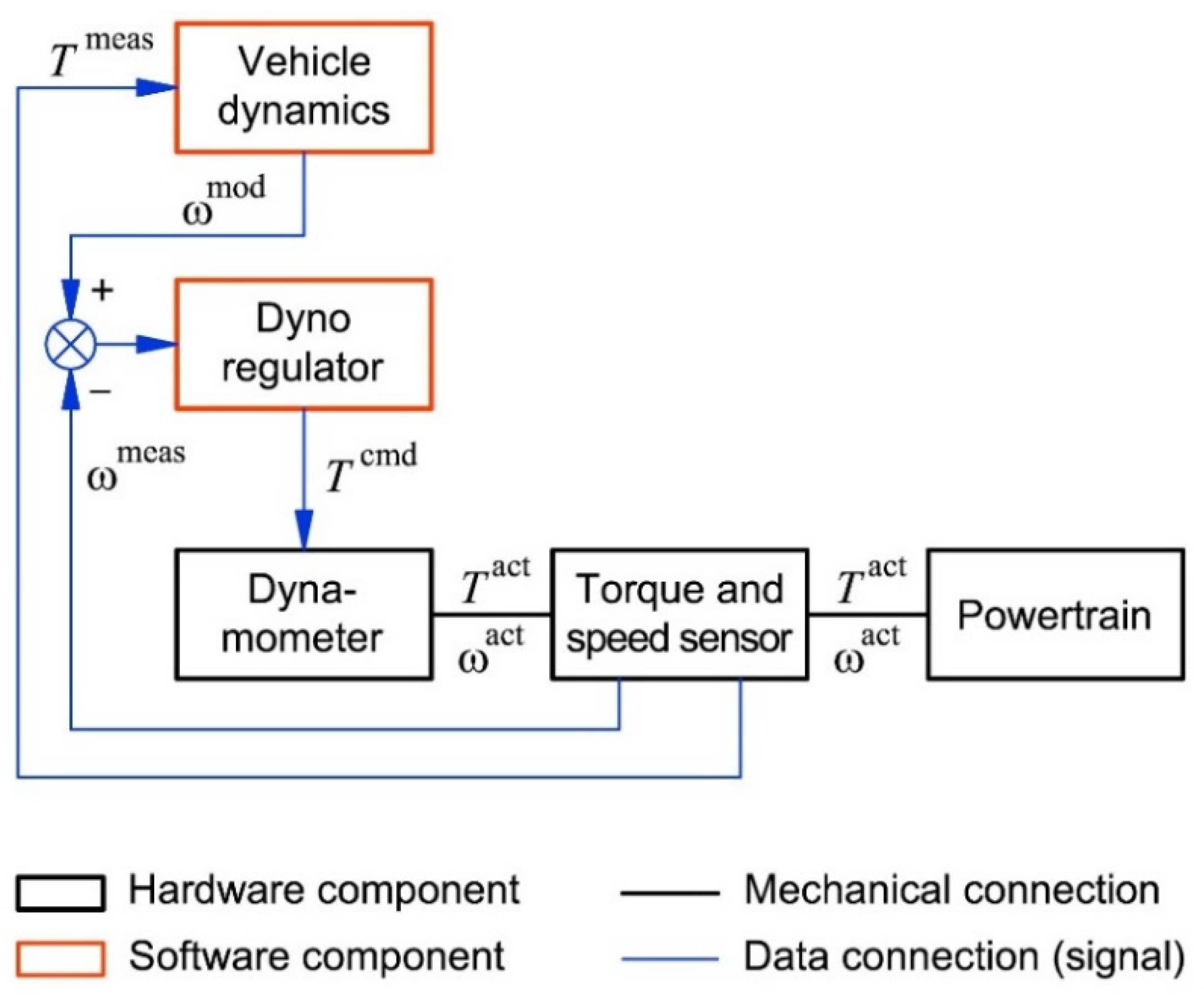
The basic CiL system shown in Figure 1 includes a hardware powertrain unit having an output shaft and a real-time software model of vehicle dynamics. These two parts are interconnected by the information and physical interfaces. In this case, the model of linear vehicle motion is considered, which is described in Section 3.1 and called the “simple” model. Simulation of a virtual inertia and other loading factors is performed by a dynamometer (for example in the form of an electric machine) connected to the powertrain’s output shaft. To provide the simulation system with feedback signals, a sensor is installed in the junction of the powertrain and dynamometer shafts that measures torque and angular speed. For adequate simulation, it is imperative that the entire tested driveline is located at one side of the sensor. The other sensor’s side is connected to the dynamometer and torque/speed transforming devices (e.g., a gearbox) if any.
To synchronize the virtual and the physical parts of the tested system, those parts are incorporated into two closed loops. The first one uses the measured shaft torque as a feedback signal that enters into the vehicle model and “drives” it. The model calculates the vehicle velocity, which is transformed into the angular speed of the powertrain output shaft and then used as the command signal for the second closed loop. The feedback of the second loop is the measured angular speed of the same shaft (its physical part). The deviation between the calculated and the measured angular speed is fed into the dynamometer regulator that calculates the torque command (or an equivalent quantity) to eliminate the deviation. The dynamometer exerts the required torque allowing to attain the commanded shaft speed. In turn, the actual values of the shaft torque and angular speed are measured by the sensor and fed back into the computing blocks therefore closing both of the loops.
The described simulation technique can be adapted for testing of powertrains having several units that drive individual axles or wheels. In the simplest case not considering tire slip, coordination of operating loads between the powertrain units is implemented using kinematic relations that include tire radii and transmission ratios. If the virtual model takes into account tire slip, the control method should be based on a relation between the kinematic variables constituting the slip. The longitudinal tire slip is a conventional variable that has several proposed options of being calculated [27]. For example, in the work [28] (p. 4), H.B. Pacejka used the following formula:
where is the wheel angular speed, is the effective rolling radius of the wheel defined either in free-rolling or in driven mode, and is the linear velocity of the wheel’s rotation center.
Regardless of the specific expression, the common feature persists across all the variants of tire slip calculation—a relation between the wheel’s angular speed and the linear speed defined in a certain point of the vehicle chassis. Additionally, one should take into account that the longitudinal tire force relates to the tire slip as follows: , where is the normal tire force and is the longitudinal tire-road adhesion coefficient being a function of the tire slip.
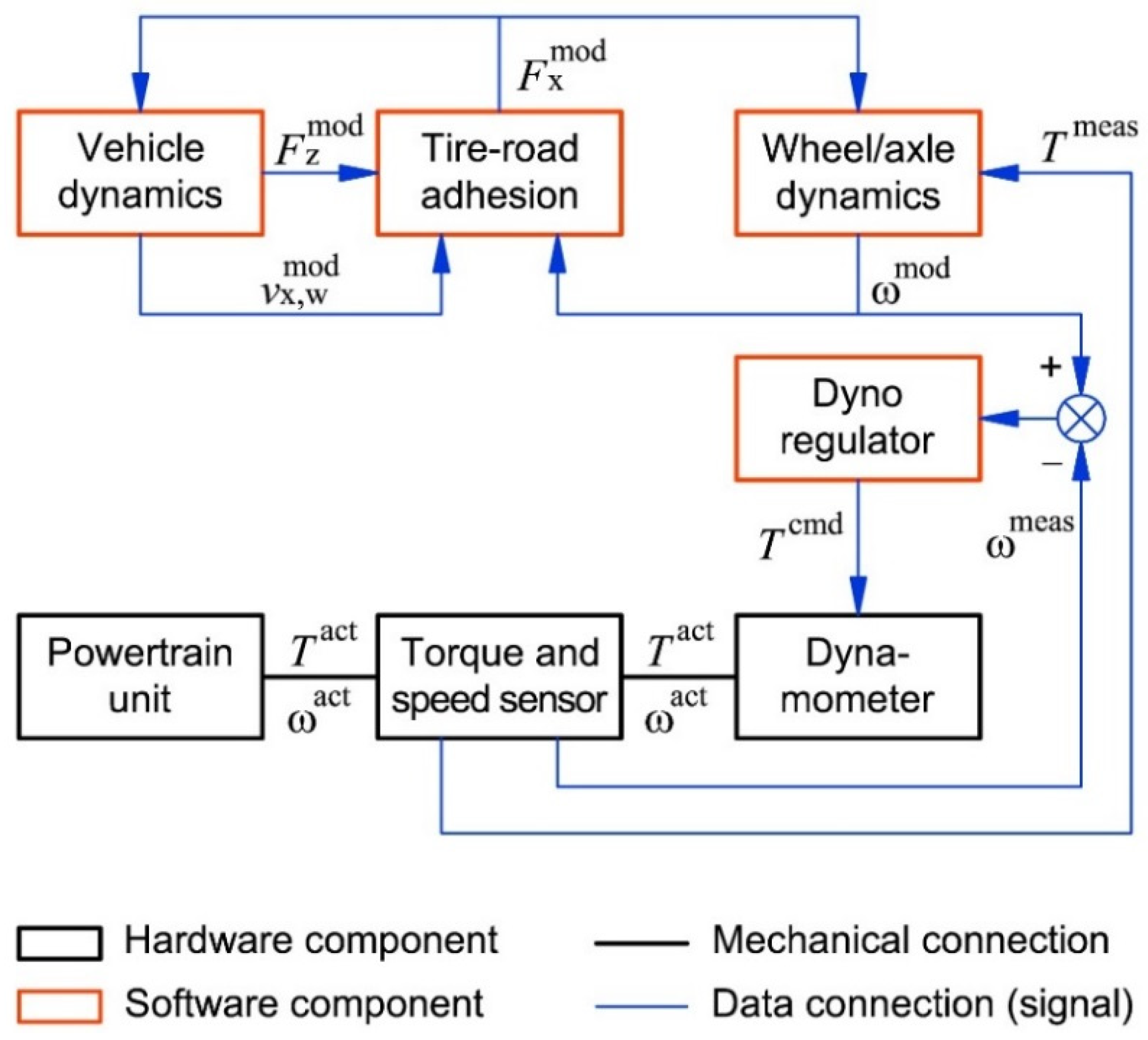
These relations suggest that, in a CiL system that has multiple drivelines associated with different wheels or axles, the central element is the model of vehicle dynamics calculating its linear velocity (see, for example, the “complex model” in Section 3.2). Rotational dynamics of all the associated wheels or axles is modeled by means of separate differential equations (also included in the “complex” model). Solving these equations yields the angular speeds of these wheels. The latter, together with the vehicle velocity, allows estimating the tire slip for all the wheels/axles. In turn, this allows calculating the longitudinal tire forces being common loading factors for vehicle dynamics and wheel dynamics. Therefore, the virtual loops become closed providing a coordination of rotation for all the simulated wheels/axles through a common “pivot”—the vehicle model. On the other hand, in regulation of the operating load of a powertrain unit, the controlled variable is the angular speed of the output shaft. The latter is defined by the angular speed of the associated axle or wheel, which is implemented as a model within the virtual part of the system. When tracking the calculated speed of the driveline shaft, the dynamometer exerts a torque corresponding to that created by the tire force and other factors acting upon the simulated wheel. Considering the described control chain, one can say that the virtual vehicle serves as a load-coordinating element for all the drivelines presented in the physical part of the system.
When elaborating a CiL simulation of a wheel or axle rotation, one can consider two options to calculate the tire slip. The first one implies using the wheel speed calculated from the measured rpms of the associated shaft in the physical part of the system. The second option is to use the wheel speed calculated by the model of wheel dynamics. Both options employ a tire model in which the longitudinal slip is an argument of the function calculating the tire force that is very sensitive to slip variation: the maximum value of the tire force is reached at 10 … 15% slip or less. Therefore, even small variations of the slip entail substantial changes in the tire force. When considering the first option, this imposes strict requirements on the precision of rpm measurement and tracking. Excessive inaccuracies could entail large variations in the calculated tire force and, consequently, in the dynamometer torque leading to its oscillations that could render the system unstable or even inflict a mechanical damage. The second option does not impose such requirements, since the slip results from the values of both the vehicle speed and the wheel speed calculated by virtual models. Hence, the accuracy of rpm tracking does not have a direct influence on the tire model. Therefore, especially in cases of a limited precision and dynamic performance of the testing equipment, the second slip estimating option can be considered as preferable.
Figure 2 illustrates the above principles implemented as the physical, simulating, and control loops of a CiL system including one hardware driveline. Other drivelines (if any) are added to the system in the same manner.
Similar techniques apply when one needs to simulate vehicle’s trajectory motion, which is characterized by certain kinematic relations between the wheels belonging to different axles and sides (i.e., right/left) of the vehicle. The main difference with the above case is the calculation of the wheel’s center linear velocity. In the simplest case not considering lateral slip, it can be calculated from so-called Ackermann’s kinematics [29] (p. 260). When the sideslip is to be considered, the lateral and yaw vehicle dynamics are simulated, and the wheel’s center velocity is calculated using the yaw rate and the sideslip angle (a detailed description can be found, for example, in [30]).
2.2. Virtual Inertia
One of the key aspects in simulation of the drivetrain’s operating load is the ratio between the inertial and the controlled (e.g., electromagnetic) portions of the loading torque. In principle, the described control techniques allow for simulation of vehicle and powertrain transient operation with no need of employing an inertial loading device (i.e., flywheel). However, a dynamometer has its own inertia constituted by the rotating parts. Also, in some types of tests, using an additional inertial device could be worthwhile. To assess the role of the dynamometer’s inertia, one can analyze the load equilibriums that take place in two types of experiments. In the first one, tire slip is neglected. The corresponding system (1) contains expressions that characterize the equilibriums of the torques and moments acting at the powertrain’s output shaft in both the physical and virtual domains, as well as the relation between the simulated inertia (in this case—the vehicle’s equivalent inertia ) and the dynamometer inertia in the form of an inequality. For simplicity, the stiffness of the shaft connecting the powertrain output to the dynamometer input is neglected.
In the physical system, the torque sensor is acted upon by the transmission output torque (from one side) and by the sum of the dynamometer’s controlled torque and its inertial moment (from other side). In the virtual system, the vehicle mass can be transformed into an equivalent flywheel () attached to the transmission output shaft, which is acted upon by the transmission output torque , measured by the physical sensor, and the calculated resistance moment representing the road load. As the dynamometer internal inertia is assumed lower than that of the vehicle, the lack of the inertial load is to be compensated by the dynamometer torque controlled by the regulator. The compensating torque should be negative (i.e., braking) when simulating a vehicle acceleration and positive (traction) during a deceleration. It should be noted that long-run transient tests, such as series of driving cycles, would require substantial amounts of energy to be exchanged with some external source if the vehicle inertia is simulated by the dynamometer torque. The optimal solution to provide such a functionality is to equip the laboratory with a rechargeable energy storage, which will consume the generated energy in accelerated- and constant speed driving and supply an energy to provide simulation of decelerations. Another solution is more traditional implying that the energy generated by the dynamometer is transmitted into an electrical net or obtained from there when the dynamometer operates in the traction mode. However, if the laboratory does not have means to regenerate energy into a net, there is no other way except to transform it into heat and dissipate. To reduce the amount of this dissipated energy, one can use an additional inertial load to simulate at least the constant part of the vehicle mass (i.e., the curb mass). In that case, the dynamometer should provide the road load and the inertial load equivalent to the transported cargo or passengers.
The system (2) includes the equilibrium expressions for a simulation considering tire slip. In that case the vehicle inertia cannot be lumped into the driveline inertia; therefore, the inertial load is only exerted by the simulated axle and/or wheels (). Other resistance factors including the vehicle equivalent inertia, tire rolling resistance, and air drag are lumped into the moment , which represents both the external and internal resistances counteracted by the tire contact force.
Since an axle or a wheel inertia is relatively small (especially when compared to that of a vehicle), one cannot exclude the case when the dynamometer inertia is larger than . When simulating an intensive tire slip accompanied by accelerations of transmission shafts, an excessive dynamometer inertia will exert a significant moment. Not corresponding to the simulated process, this moment should be compensated by the controlled torque, which can be called a “negative virtual inertia.” To avoid such a complication, it is preferable that, in an experiment considering tire slip, the dynamometer inertia does not exceed the simulated inertia by far. One cannot exclude the opposite case when the dynamometer inertia is significantly smaller than that of the simulated driveline. Compensating this “inertia deficiency” implies that the dynamometer should exert a “positive virtual inertia” using the controlled torque. This will require of the dynamometer to have a fast time response when simulating an intensive tire slip. If the dynamometer does not meet this requirement, an additional inertial load could be attached to its shaft allowing to exclude the higher frequency range from transient processes. Obviously, the optimum value of the additional inertia would be that making the total inertia of the dynamometer equal to or close to it.
It should be emphasized that the described dynamometer control techniques are based on the tracking error compensation principle, which does not require taking into account the dynamometer inertia and the inertia of an additional flywheel (if any) in calculating the “virtual inertia,” since this is done automatically as a part of the error compensation principle. A simulation of an operating load does not require knowing the values of these inertias. Some published works suggest compensating the dynamometer inertia by subtracting its calculated moment from the torque measured by the shaft sensor. In no way such a “compensation” will affect the closed loop control, as it exerts the torque corresponding to the virtual inertia automatically when reacting to the rpm error. Therefore, instead of eliminating the dynamometer inertia from the simulation, a “compensation” will change the simulated vehicle mass. As an illustration, one can imagine an extreme case, when the dynamometer inertia is close to that of the vehicle, for example 90% of that. Subtracting the inertial moment from the measured torque will make the simulated vehicle mass diminish by 90%. If the torque acting at the transmission output shaft yields an angular acceleration equal to, for example, 1 (unit acceleration), the measured value of that torque will “drive” the simulated vehicle with an acceleration equal to 10. In response, the regulator of the dynamometer will exert the controlled torque in an attempt to accelerate the dynamometer inertia accordingly (i.e., ten times faster). As a result, instead of the desired vehicle mass the system will imitate a vehicle ten times lighter, but with ten times higher dynamometer torques due to a necessity of accelerating its large inertia. One can also find examples of compensating the inertia of the components constituting the physical part of the tested powertrain by adding this inertia to the virtual model. This is incorrect, as this inertia is included in the torque measured by the shaft sensor.
3. Mathematical Models of Vehicle Dynamics for CiL Systems
3.1. “Simple” Model
The virtual part of a CiL system for powertrain testing should include at least a model of vehicle dynamics. The complexity of this model depends on driving modes to be simulated by the CiL system. Another criterion is whether tire slip should be taken into account. The simplest case implies linear motion of the vehicle with the tire slip neglected. This approach is suitable for simulation of driving cycles, which, generally, do not contain steering maneuvers and imply driving with moderate accelerations at high adhesion road surfaces, i.e., conditions in which a substantial tire slip does not occur. To simulate such regimes, one can use a model of vehicle dynamics (hereafter referred to as the “simple” model) describing a linear motion of one lumped mass expressed as follows:
where is the vehicle longitudinal velocity; is the total torque exerted at the vehicle’s driving wheels; is the force equivalent to the total rolling resistance of the vehicle’s tires; is the air drag force; is the longitudinal projection of the gravity force when driving at inclined road surfaces; is the vehicle’s mass; is the number of the vehicle’s wheels; is the wheel inertia; is the wheel geometric radius.
The expression for the rolling resistance force is derived by lumping the rolling resistance moments of all the vehicle tires under the assumption of their mutual equality. The resulting expression reads , where is the gravity constant and is the rolling resistance coefficient. The latter depends on several factors, however, under assumptions of a moderate wheel torque, absence of tire sideslip, normal operating tire temperature and pressure, it can be approximated as a function of the wheel’s center linear velocity (in the “simple” model, it is equal to that of the vehicle) and the type of road surface [31] (pp. 43–44): , where is the rolling resistance coefficient at near-zero velocity, is the gain of the quadratic velocity term, and is the additional rolling resistance associated with the type of the road surface (e.g., asphalt, snow, ice, etc.,).
The gravity force projection onto the road surface is proportional to the vehicle weight and the road inclination angle : . The air drag force can be calculated using the well-known empirical formula [31] (p. 96) , where is the vehicle longitudinal air drag coefficient, is the frontal area of the vehicle, and is the air density.
3.2. “Complex” Model
A typical example of a testing task requiring a more detailed model is simulation of trajectory maneuvers taking into account the limited tire-road adhesion. Such driving modes could be used to assess the powertrain performance in such tasks as traction control and torque vectoring. This requires taking into account the tire slip in both the longitudinal and lateral directions that entails modeling the vehicle trajectory motion and the wheel angular motion as independent dynamic processes linked by kinematic relations. When designing a CiL system, it is advisable to elaborate a model that delivers such a functionality while being a reasonable trade-off between an accuracy, complexity, and calculating burden. As an example, one can propose the model used in the CiL system developed for the case study described in Section 4. It consists of six lumped masses, namely, the vehicle mass performing trajectory motion and having three degrees of freedom, the sprung mass performing roll motion, and four rotating wheel masses. The equations of this model are derived from schematics describing the mentioned types of motion. The schematics are omitted in this article, however, an interested reader is referred to the publication that contains those schematics along with a detailed description of the model [30] (similar models can also be found in the publications dedicated to vehicle dynamics, for example in [29] (pp. 303–309)). The differential equations derived from the said schematics can be aggregated into the following system (hereafter referred to as the “complex” model):
where and are the longitudinal and lateral components of the acceleration vector in the vehicle’s center of gravity; and are the longitudinal and lateral components of the linear velocity vector in the vehicle’s center of gravity; is the vehicle yaw rate; and are the longitudinal and lateral projections of the tire force onto the vehicle coordinate axes; is the vehicle yaw inertia; is the yawing moment exerted by the tire force; is the roll inertia of the vehicle’s sprung mass; is the height of the vehicle’s center of gravity above the road surface; is the roll angle of the sprung mass; and are respectively the roll stiffness and damping coefficient of a suspension; is the longitudinal projection of the tire force onto the wheel coordinate axes.
In the system (3), the variables associated with individual wheels or axles are provided with indices i and j. The former is the number of the axle, while the latter is the number of the wheel associated with the i-th axle (meaning that each axle has its own wheel numeration). The total number of the vehicle axles is denoted by n, while is the total number of the wheels associated with the i-th axle. Note that the last line of the system (3) corresponds to the ij-th wheel meaning that this line actually represents the array of equations describing rotational dynamics of all the modeled vehicle wheels.
The components of a tire force vector are calculated using functions of the tire longitudinal slip and the sideslip angle. These functions constitute the tire-road adhesion model, which can be selected from the existing variety [28] (pp. 81–85). In the case study described below, a well-known semi-empirical model called the Magic Formula devised by H.B. Pacejka [28] (pp. 165–183) was employed. The detailed descriptions of the kinematic relationships for the tire longitudinal slip and the sideslip angle are presented in the work [30], as well as the equations projecting the tire force components from the wheel-bound coordinate system onto the vehicle-bound coordinate system. The normal tire forces are calculated using a static equilibrium of moments involving the body-roll moment built by the suspensions and calculated from the body roll equation (i.e., the fourth equation of the system (3)).
The described models are merely examples of “simple” and “complex” solutions that can be employed in a CiL system intended for powertrain testing. Other types of models are possible, for example, putting emphasis on suspensions and road unevenness or having more/less degrees of freedom, etc. The choice is defined by specific testing tasks for which the elaborated CiL system is intended.
4. Case Study
4.1. The Object and the Tasks
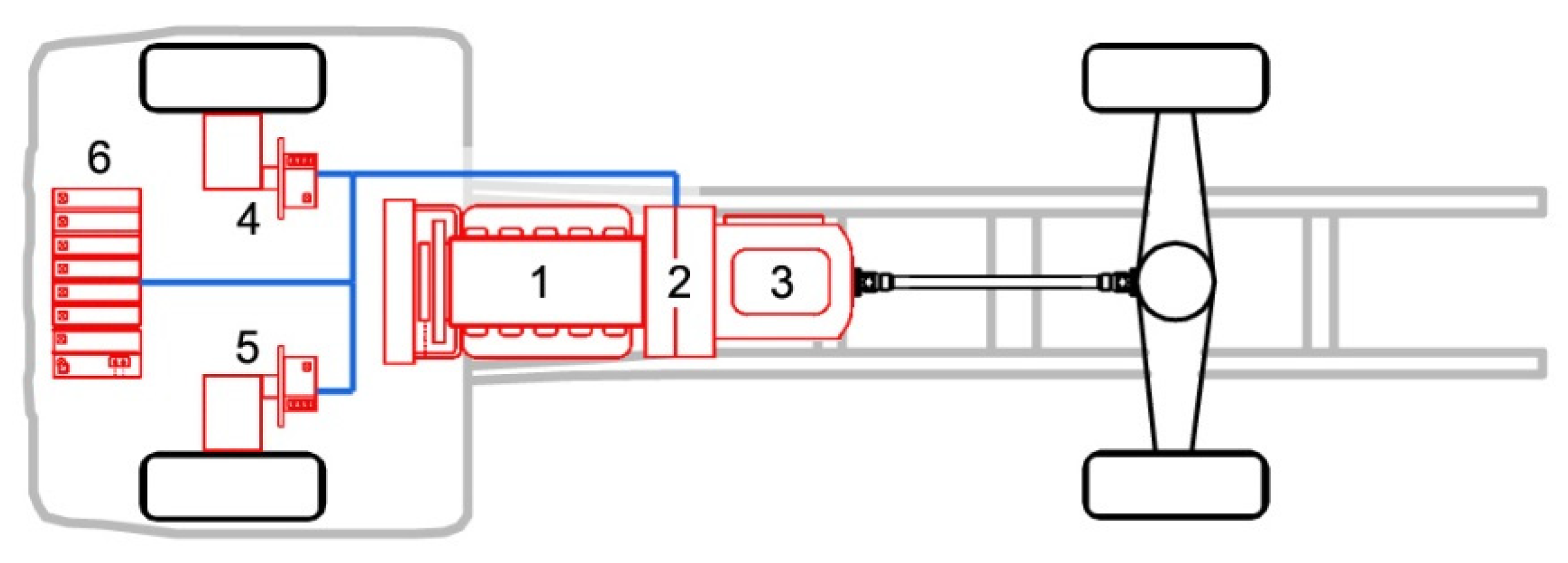
The case study was conducted as a part of a project aimed at development of a heavy-duty hybrid electric vehicle (specifically, a tractor for an articulated vehicle) intended for long haulage. A schematic of its powertrain is shown in Figure 3. The main components are highlighted in red. The blue lines depict high-voltage connections.
The powertrain belongs to an all-wheel-drive type. The main driveline connected to the rear axle has the parallel hybrid topology. It consists of an internal combustion engine 1 (diesel), a so-called hybrid module 2, and an automated mechanical gearbox 3 (also called a robotized gearbox).
The main components of the hybrid module are a traction electric machine and an automated clutch housed by a common casing (see for example [32,33]). The electric machine has the maximum power and torque that, together with a multispeed gearbox, provide the vehicle with a wide range of pure electric traction and regenerative braking when the engine is disconnected from the transmission. When the module’s clutch is engaged, both the engine and the electric machine are connected to the gearbox providing the hybrid mode. If the traction battery needs replenishing, the engine produces a surplus power that is then drawn by the electric machine, which operates in the generation mode. The electric machine of a hybrid module also performs the synchronizing operation when the gearbox is shifting: during an upshift, it exerts a braking torque that decelerates the input shaft of the gearbox, and accelerates that shaft when downshifting. The front electric motors are intended for auxiliary features like an additional traction when driving uphill or at low-adhesion surfaces. They also provide regenerative braking. Table 1 summarizes the main characteristics of the powertrain components.
The goal of the work presented by this article was to develop a system for laboratory testing of the said hybrid powertrain allowing to study its characteristics and to elaborate or calibrate its control system in different operating conditions: driving cycles, driving at surfaces with limited tire adhesion, handling maneuvers.
4.2. Component-in-the-Loop System Design and Implementation
4.2.1. Design Concept
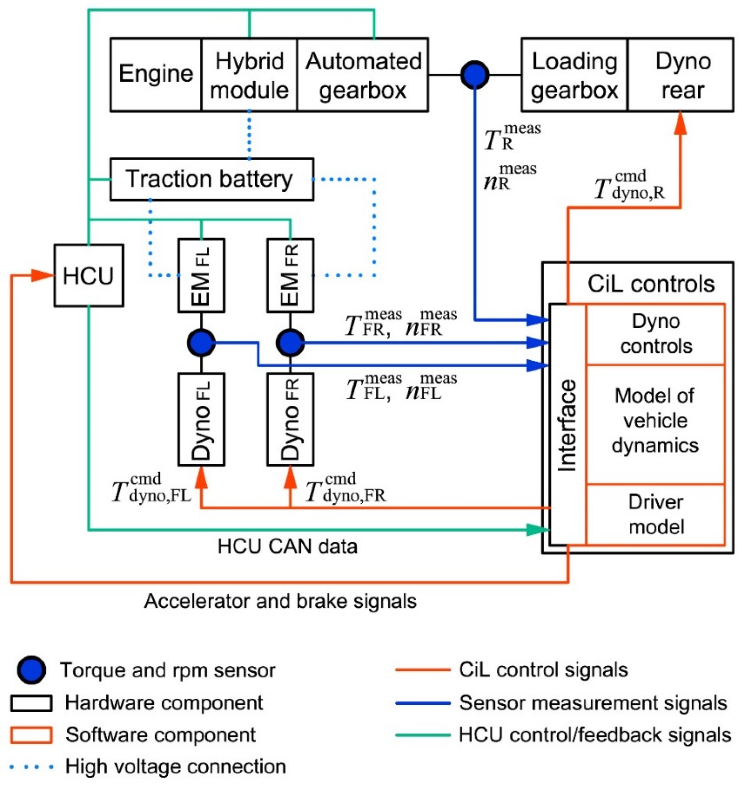
The principle described in Section 2.1 for powertrains having several drivelines says that the coordinated simulation of operating loads is implemented using a model of vehicle dynamics having its wheels or axles involved in a closed loop control of the dynamometers associated with the tested physical drivelines. Based on this principle, a component-in-the-loop system has been developed for laboratory testing of the hybrid powertrain. Figure 4 shows a schematic of that system.
The physical part of the CiL system contains all the above-described powertrain components except for the reduction gears of the front electric machines. The physical interaction between the hardware and the software parts of the CiL system is provided by the loading devices connected to the output shaft of the rear driveline (“Dyno rear”) and to each of the front electric machines (“Dyno FR” and “Dyno FL”, where “FR” stands for “front right” and “FL” for “front left”). The torque and rpm sensors embedded between the shafts of the powertrain units and the loading devices provide feedbacks for the virtual part of the CiL system and for the regulators of the loading devices. The block called “Loading gearbox” corresponds to a multispeed manual gearbox placed between the rear driveline and the rear dynamometer in order to match the loading range to the simulated driving conditions. The need of using this gearbox was due to a wide torque range seen at the output shaft of the automated gearbox, which could not be fully handled by the electric machine used as the rear loading device.
The schematic also shows a hardware device called Hybrid Control Unit (HCU) that contains the top-level powertrain control system connected to the local controllers by bilateral data lines using CAN protocol. The local controllers (not shown in Figure 4 as separate devices) are associated with each of the powertrain components providing the management of their operation and/or monitoring of their parameters.
The “CiL controls” block constitutes a hardware controller containing software implementations of the virtual model and the regulators of the loading devices, as well as the means to communicate with the external controlling and measurement equipment. The data wires connecting the CiL controller to the surrounding equipment are shown as the color lines having the arrows that indicate the directions of the data flows. The lines with no arrows correspond to bilateral data flows. Inside the controller, the “Interface” block houses both hardware and software means to receive the feedback signals from the measuring equipment (i.e., the shaft torques , , and rpms , , ) and the HCU (CAN bus signals), and to transmit the command signals into the local controllers of the dynamometers and into the HCU (the accelerator and brake signals). The “Dyno controls” block contains a software implementation of the three regulators controlling the rpms of the rear driveline and the front electric machines by means of the torque commands for the corresponding dynamometers (, , ).
The CiL controller stores a software implementation of the mathematical models constituting the virtual part of the tested system and runs those models in real-time. Depending on testing task, the system’s operator can choose between the above-described “simple” model intended for driving cycles and the “complex” model intended for dynamic maneuvers.
Depending on the selected vehicle model, the “Driver model” block activates one or two control loops. The first loop regulates the velocity of the virtual vehicle using a reference signal (for example, a velocity value required by a driving cycle) and the feedback signal being the longitudinal component of the vehicle velocity calculated by the model. The discrepancy between these variables is eliminated by means of two regulators outputting the command values for the accelerator and the brake pedals. Since those pedals are not physically presented in the CiL system, their command signals are fed directly into the HCU. Therefore, the velocity control loop contains both software models and physical devices making the hardware powertrain “drive” the virtual vehicle. When a simulation of handling maneuvers is required, an additional control loop is activated that allows the virtual vehicle to drive along predefined trajectories. A subroutine of this program module estimates a linear deviation of the vehicle’s path from the reference trajectory, and then feeds the tracking error into the regulator that calculates the steering wheel angle eliminating the deviation. The value of that angle is transmitted into the model of vehicle dynamics as a control input. Therefore, the second loop is purely virtual and has no direct effect on the hardware part of the system. However, it influences the operation of the tested powertrain indirectly—via the vehicle kinematics that defines the angular speeds of the powertrain shafts entailing a reaction of the powertrain controls.
4.2.2. Implementation
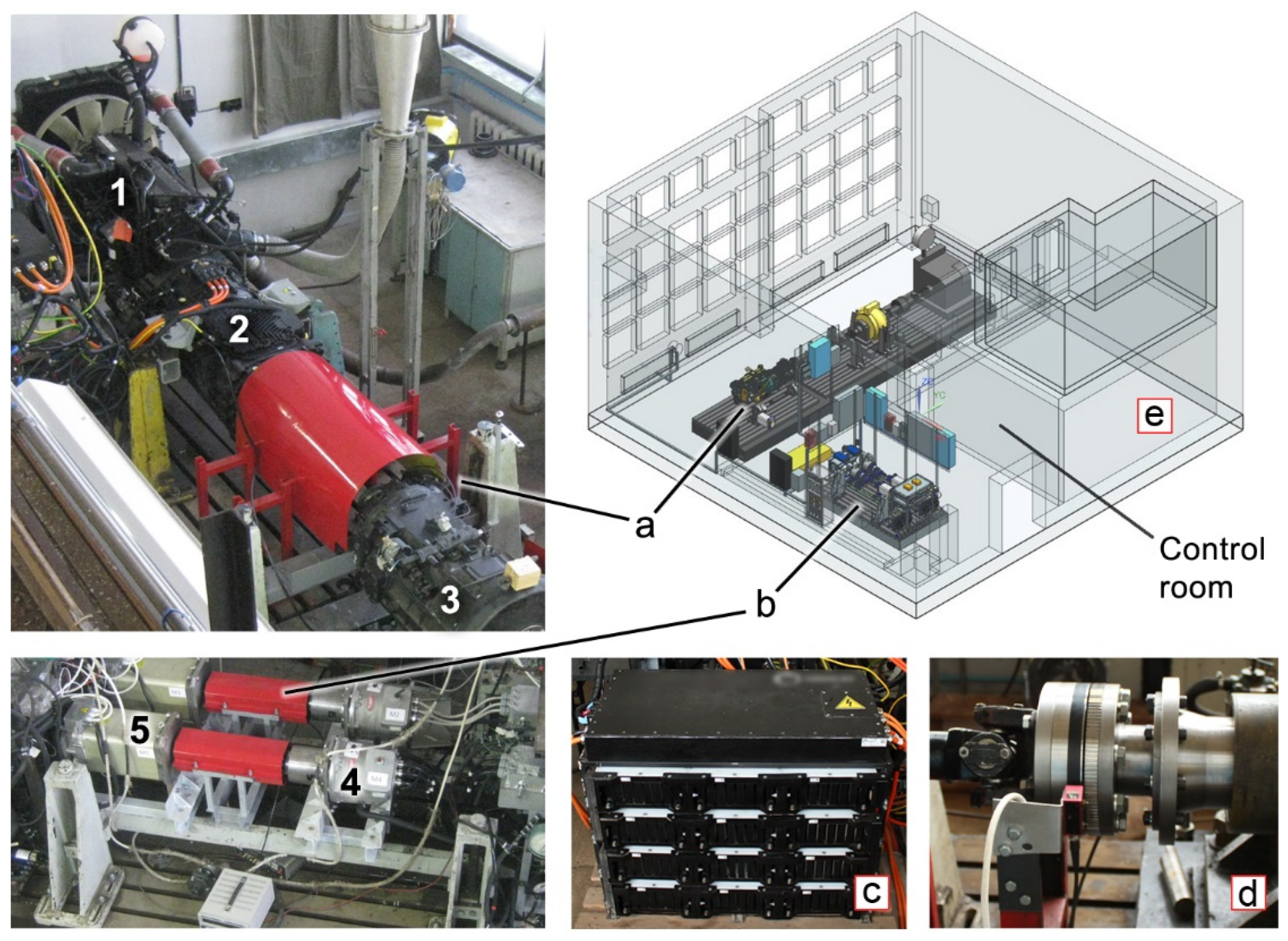
The CiL system has been built in a laboratory intended for powertrain testing. The hardware part consists of two test benches, one of which houses the rear driveline and its load simulating equipment (Figure 5a), while the second one contains the front electric drives and their loading devices (Figure 5b). The power electronics, the traction battery (Figure 5c), and the auxiliary equipment are placed between the test benches. Absence of mechanical connections between the front and the rear drivelines allowed mounting them inside the laboratory independently of their arrangement at the chassis of an actual vehicle, which is illustrated by the CAD model shown in Figure 5e.
Physical interfacing between the powertrain components and the virtual model is provided by the electric machines capable of operating in traction and generations modes. In the junctions of the powertrain units and the loading devices, sensors were installed providing the torque and speed feedback. One of them, belonging to the rear driveline’s test bench, is shown in Figure 5d.
4.3. Component-in-the-Loop Testing Results
To evaluate the functionality of the developed CiL system, series of tests were conducted in the driving modes listed in Section 4.1. The main parameters of the simulated vehicle are summarized in Table 2 corresponding to those of a typical artic (tractor).
The test type to be performed first was a driving cycle. The vehicle model used in that case within the CiL controller was the “simple” one implying a lumped single-mass vehicle moving linearly. Therefore, in the “Driver model” block, only the linear velocity control loop was active.
For a heavy-duty hybrid vehicle, one can consider the transient cycle defined by the UNECE Regulation No 49 [34] as a representative driving schedule when speaking of its version plotting the vehicle velocity against time. In regard of the covered operating range of a vehicle, the urban part of the cycle is the most interesting, as it implies the full ratio range of the automated gearbox to be in use, which, in turn, makes the engine and the hybrid module deliver their functions in broad ranges of torque and rpms (due to a close association of their operating regimes with that of the gearbox).
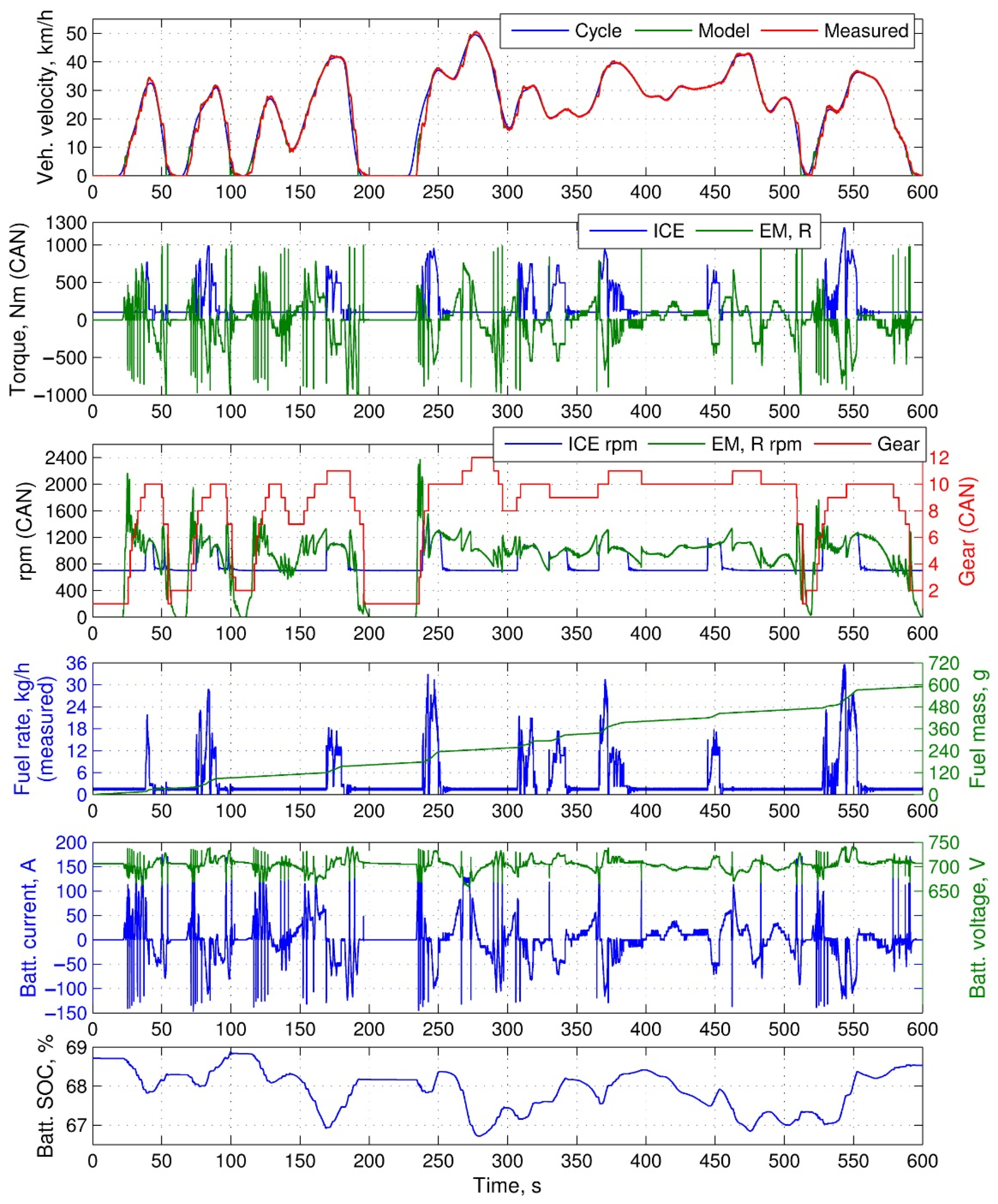
The testing series consisted of ten runs in the urban driving cycle. Some of the variables logged in one of those runs are shown in Figure 6 demonstrating a comprehensive picture of the hybrid powertrain operation. From the top to the bottom of the figure, one can see the following graphs: the vehicle velocity prescribed by the cycle schedule, calculated by the model of vehicle dynamics, and calculated from the rpm measurements at the rear output shaft; the torques and rpms of the internal combustion engine (ICE) and the rear traction electric machine (EM, R), as well as the number of the engaged gear obtained from the CAN bus; the measured engine fuel rate and the mass of the consumed fuel; the traction battery current, voltage, and the state of charge (SOC) obtained from the CAN bus (specifically, from the battery management system).
The driving cycle tests have shown that the synchronization of the virtual and physical parts of the CiL system is stable and sufficiently accurate in terms of tracking the rpm of the output shaft calculated by the model. The driver model also performs with an acceptable accuracy having the velocity tracking error whose average does not exceed 2 km/h, which conforms to typical requirements of the technical standards that include driving cycle tests. In the graphs of the electric machine torque and the battery parameters, one can notice a number of spikes that indicate gear-synchronizing events mentioned in Section 4.1.
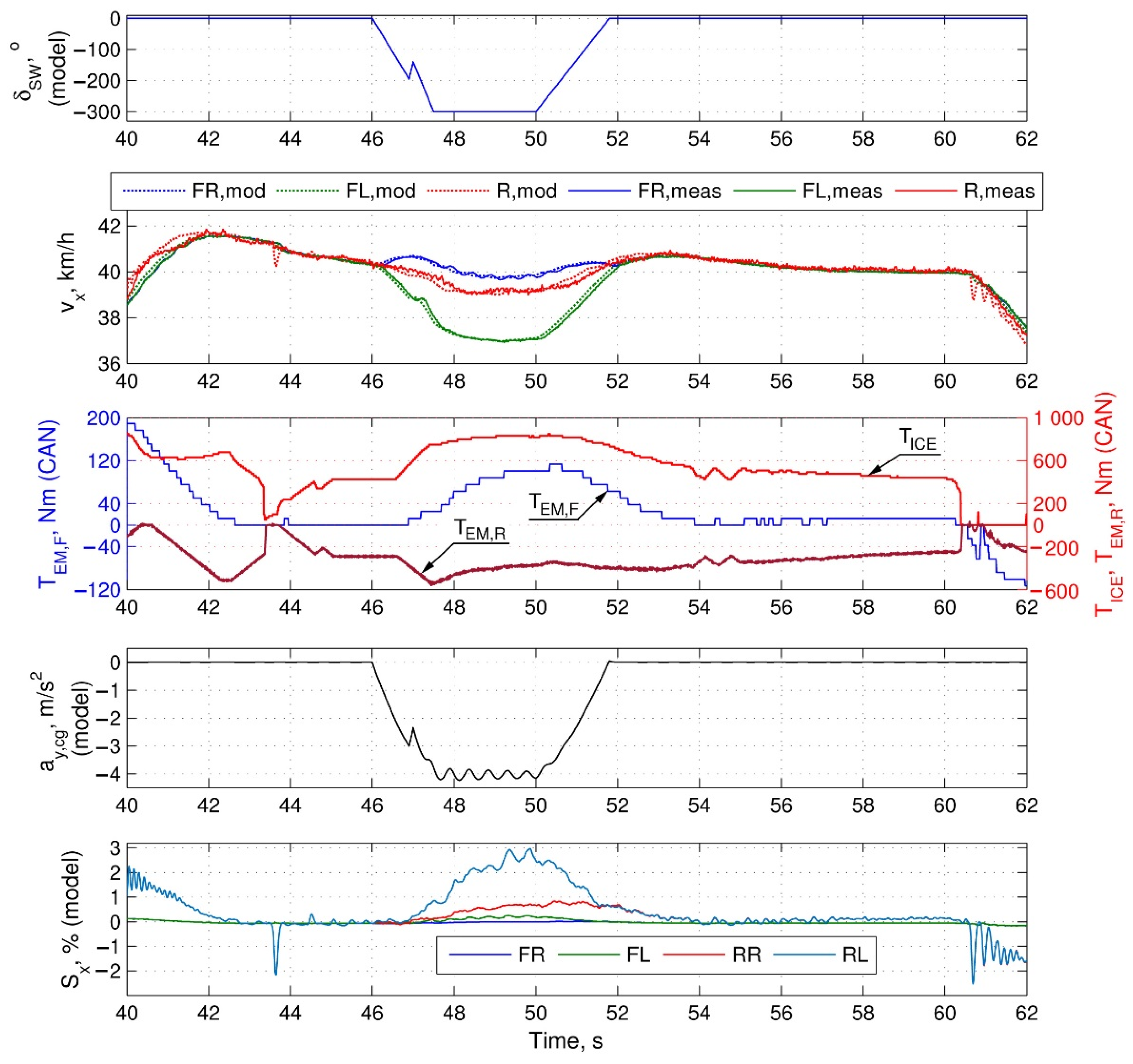
The testing series simulating trajectory motion taking into account the tire-road adhesion included two handling maneuvers, namely, “turn” and “lane change.” In the CiL controller, the “complex” vehicle model was selected to simulate trajectory motion with the tires slipping in the longitudinal and lateral directions. The additional controlling loop was activated in the driver model for path tracking. Figure 7 demonstrates the results of a test that simulated a turn having a radius of 35 m at a dry asphalt road with the maximum adhesion coefficient of 0.9. The plots show the following variables (from top to bottom): the calculated steering wheel angle (); the linear velocities () of the front wheels (FR and FL) and the rear axle (R) calculated by the model (mod) and measured using the rpm sensors (meas); the torques of the engine (), the rear electric machine (), and the front electric machines () obtained from the CAN bus; the lateral acceleration in the vehicle’s center of gravity () calculated by the model; the values of the longitudinal tire slip () calculated by the model for all the vehicle wheels.
From the presented graphs, one can see that, when simulating the turn, both the vehicle model and the hardware powertrain components were operating adequately showing the correct kinematic relations between the wheel speeds. Since a left turn was simulated, the front right wheel was in the outer position (in relation to the center of the turn), hence being the outrunning one, while the front left wheel was in the inner position therefore having a lower speed. One can also see that the calculated slip of the rear left wheel was larger than those of the other wheels were. That occurred due to two factors, namely, a redistribution of the normal forces in the virtual model and an increase of the engine torque in the hardware part of the rear driveline (in order to keep the required speed the driver model increased the accelerator signal). That combination of the physical and virtual factors resulted in an increase of the torque and lowering of the weight acting at the rear left wheel, which, in turn, entailed a higher calculated slip. This is an illustration of the mutual influence between the virtual and the physical factors affecting the simulated vehicle behavior.
5. Conclusions
Resuming the study described in the article, one can highlight its key methodical and practical results. The theoretical analysis has three main outcomes contributing to the CiL methodology. These can be formulated as follows.
- When considering all-wheel-drive powertrains having functions that deal with vehicle active safety and dynamics, the CiL system is supposed to simulate vehicle maneuvers at road surfaces with a limited tire adhesion. In that case, one can use the described principle of synchronizing the operating loads between different drivelines of the powertrain taking into account their independent rotation due to tire slip or/and kinematics of trajectory motion. The principle is based on the cyclic relations between the vehicle velocity and the wheel speed stemming from the tire slip and the longitudinal tire force. The latter is a function of the slip, and simultaneously, the common acting factor for both the vehicle- and wheel dynamics. Therefore, the simulating loops sharing the common vehicle velocity and the individual angular speeds of the wheels generate the rpm commands for the dynamometers connected to the physical drivelines resulting in their synchronization in accordance with the simulated driving mode. The model of vehicle dynamics serves as a synchronizing “pivot” for the speed regimes of the modeled wheels (or axles) and the loading regimes of the hardware drivelines associated with those wheels.
- The analysis and clarification of the “virtual inertia” principle allows concluding that when an inertia is simulated by means of a closed loop control of the drivetrain’s shaft angular speed, it does not need to be taken into account or compensated in any additional way—neither in the vehicle model, nor in the CiL control system. If the virtual inertia is intended to simulate the vehicle mass then, in the virtual model, the vehicle should have the same mass as in an actual road test (i.e., no mass correction is required). The torque feedback signal provided by the shaft-mounted sensor “drives” the virtual vehicle, while the shaft angular speed feedback makes the dynamometer exert an operating load corresponding to the sum of the resistance forces including the inertial one.
- If the laboratory equipment employed in the CiL system is limited in terms of precision and time response, one can resort to the described method of tire slip simulation having low sensitivity to errors of measurement equipment and actuating mechanisms. The method implies that the slip is estimated using the calculated value of the wheel angular speed rather than that derived from the measured shaft rpm. This makes calculation of the tire force less dependent on hardware inaccuracies, therefore avoiding errors in the loading torque exerted by the dynamometer. When using the calculated quantity of the angular speed, the hardware equipment of a CiL system will simulate tire slip to the extent of accuracy allowed by its construction, hardware errors will not have a significant influence on this process.
The said methodical outcomes has been implemented in a laboratory facility for testing of a hybrid powertrain that features individual driving of the rear axle and each of the front wheels. The tests simulating vehicle operation in a driving cycle and in trajectory maneuvers have demonstrated an adequate and accurate interaction between the virtual vehicle and the hardware powertrain, therefore verifying the design and operating approaches described and analyzed in the theoretical part of the study.
When considering future applications of the presented methodology, one can draw the following conclusions. Being based on universal and scalable simulating and control methods, the described techniques are versatile and can be applied to different kinds of powertrains including conventional and alternative with different numbers of driving axles and wheels, belonging either to heavy-duty or light-duty vehicles. Various powertrain functions can be developed or studied be means of the described CiL approaches including coordinated control of driveline components, traction control, and yawing moment control. Better understanding of the CiL design and operating principles stemming from the methodical outcomes of the study should help researchers and developers to elaborate systems that adequately and accurately replicate powertrain functioning in miscellanea of driving conditions.
Author Contributions
Conceptualization, I.K.; methodology, I.K.; software, I.K. and A.K.; validation, I.K., and S.K.; formal analysis, I.K. and A.K.; investigation, I.K. and S.K.; resources, S.K.; data curation, I.K.; writing—original draft preparation, I.K.; writing—review and editing, I.K. and U.A.; visualization, I.K.; supervision, S.K.; project administration, S.K., A.T., and K.K.; funding acquisition, S.K., U.A., A.T., and K.K. All authors have read and agreed to the published version of the manuscript.
Funding
The case study was funded under the terms of the agreement #12411.0810200.20.B26 with the Ministry of industry and trade of Russian Federation.
Institutional Review Board Statement
Not applicable.
Informed Consent Statement
Not applicable.
Data Availability Statement
Not applicable.
Conflicts of Interest
The authors declare no conflict of interest.
Abbreviations
| CAD | Computer aided design |
| CAN | Controller area network |
| CiL | Component-in-the-Loop |
| EM | Electric machine |
| FL, FR | Front left, front right |
| HCU | Hybrid Control Unit |
| ICE | Internal combustion engine |
| R | Rear (index) |
| SOC | State of charge |
| UNECE | United Nations Economic Commission for Europe |
References
- Isermann, R. Fahrdynamik-Regelung. Modellbildung, Fahrerassistenzsysteme, Mechatronik; Friedr. Vieweg & Sohn Verlag|GWV Fachverlage GmbH: Wiesbaden, Germany, 2006; pp. 169–211. [Google Scholar]
- Bakhmutov, S.V.; Ivanov, V.G.; Karpukhin, K.E.; Umnitsyn, A.A. Creation of operation algorithms for combined operation of anti-lock braking system (ABS) and electric machine included in the combined power plant. IOP Conf. Ser. Mater. Sci. Eng. 2018, 012003. [Google Scholar] [CrossRef] [Green Version]
- Shorin, A.A.; Karpukhin, K.E.; Terenchenko, A.S.; Kondrashov, V.N. Traction module of cabless unmanned cargo vehicles with electric drive. Int. J. Mech. Eng. Technol. 2018, 9, 1903–1909. [Google Scholar]
- Herring, J.A.; Burnham, K.J.; Oleksowicz, S. Review and Simulation of Torque Vectoring Yaw Rate Control. In Proceedings of the International Conference on Systems Engineering (ICSE), Coventry, UK, 11–13 September 2012. [Google Scholar]
- Goggia, T.; Sorniotti, A.; De Novellis, L.; Ferrara, A.; Pennycott, A.; Gruber, P.; Yunus, I. Integral Sliding Mode for the Yaw moment Control of Four-Wheel-Drive Fully Electric Vehicles with In-Wheel Motors. Int. J. Powertrains 2015, 4, 388–419. [Google Scholar] [CrossRef]
- Albers, A.; Düser, T. Implementation of a Vehicle-in-the-Loop Development and Validation Platform. Automobiles and sustainable mobility. In Proceedings of the FISITA 2010 World Automotive Congress, Budapest, Hungary, 30 May–4 June 2010. [Google Scholar]
- Tibba, G.; Malz, C.; Stoermer, C.; Nagarajan, N.; Zhang, L.; Chakraborty, S. Testing Automotive Embedded Systems under X-in-the-loop Setups. In Proceedings of the IEEE/ACM International Conference on Computer-Aided Design (ICCAD ’16), Austin, TX, USA, 7–10 November 2016. [Google Scholar] [CrossRef]
- Ivanov, V.; Augsburg, K.; Bernad, C.; Dhaens, M.; Dutré, M.; Gramstat, S.; Magnin, P.; Schreiber, V.; Skrt, U.; van Kelecom, N. Connected and Shared X-in-the-Loop Technologies for Electric Vehicle Design. World Electr. Veh. J. 2019, 10, 83. [Google Scholar] [CrossRef] [Green Version]
- Fegraus, C.E.; D’Angelo, S. Inertia and Road Load Simulation for Vehicle Testing. Patent US 4,161,116, 21 September 1977. [Google Scholar]
- Henry, K.J.; Kotwicki, A.J. Emulation System for a Motor Vehicle Drivetrain. Patent US 4,680,959, 23 April 1986. [Google Scholar]
- Lang, T.; Schyr, C. Simulation Aided Process for Developing Powertrains. In Proceedings of the SAE Brazil Convention 2000 (International Mobility Technology Conference and Exhibit), Sao Paulo, Brazil, 2–4 October 2000. [Google Scholar]
- Scordia, J.; Trigui, R.; Desbois-Renaudin, M.; Jeanneret, B.; Badin, F. Global Approach for Hybrid Vehicle Optimal Control. J. Asian Electr. Veh. 2009, 7, 1221–1230. [Google Scholar] [CrossRef] [Green Version]
- Trigui, R.; Jeanneret, B.; Malaquin, B.; Plasse, C. Performance Comparison of Three Storage Systems for Mild PHEVs Using PHIL Simulation. IEEE Trans. Veh. Technol. 2009, 58, 3959–3969. [Google Scholar] [CrossRef] [Green Version]
- Wu, J.; Dufour, C.; Sun, L. Hardware-in-the-Loop Testing of hybrid vehicle motor drives at Ford Motor Company. In Proceedings of the IEEE Vehicle Power and Propulsion Conference, Lille, France, 1–3 September 2010. [Google Scholar] [CrossRef]
- Kaup, C.; Pels, T.; Ebner, P.; Ellinger, R.; Gschweitl, K.; Loibner, E.; Schneider, R.; Walter, L. Systematic Development of Hybrid Systems for Commercial Vehicles; SAE Technical Paper 2011-28-0064; SAE: Warrendale, PA, USA, 2011. [Google Scholar] [CrossRef]
- Sheng-bing, Y.; Zhen-zhen, L.; Feng, X.; Guo-guang, Z.; Yuan-fa, D.; Jun, W. A Electric Vehicle Powertrain Simulation and Test of Driving Cycle Based on AC Electric Dynamometer Test Bench. In Proceedings of the 2012 International Conference on Mechanical Engineering and Material Science (MEMS 2012), Yangzhou, China, 16–18 December 2012; pp. 273–276. [Google Scholar] [CrossRef] [Green Version]
- Li, W.; Shi, X.; Guo, D.; Yi, P. A Test Technology of a Vehicle Driveline Test Bench with Electric Drive Dynamometer for Dynamic Emulation; SAE Technical Paper 2015-01-1303; SAE: Warrendale, PA, USA, 2015. [Google Scholar] [CrossRef]
- Klein, S.; Xia, F.; Etzold, K.; Andert, J.; Amringer, N.; Walter, S.; Blochwitz, T.; Bellanger, C. Electric-Motor-in-the-Loop: Efficient Testing and Calibration of Hybrid Power Trains. IFAC-PapersOnLine 2018, 51, 240–245. [Google Scholar] [CrossRef]
- Vafaeipour, M.; El Baghdadi, M.; Verbelen, F.; Sergeant, P.; Van Mierlo, J.; Hegazy, O. Experimental Implementation of Power-Split Control Strategies in a Versatile Hardware-in-the-Loop Laboratory Test Bench for Hybrid Electric Vehicles Equipped with Electrical Variable Transmission. Appl. Sci. 2020, 10, 4253. [Google Scholar] [CrossRef]
- Jiang, S.; Smith, M.; Kitchen, J.; Ogawa, A. Development of an Engine-in-the-Loop Vehicle Simulation System in Engine Dynamometer Test Cell; SAE Technical Paper 2009-01-1039; SAE: Warrendale, PA, USA, 2009. [Google Scholar] [CrossRef] [Green Version]
- Klein, S.; Savelsberg, R.; Xia, F.; Guse, D.; Andert, J.; Blochwitz, T.; Bellanger, C.; Walter, S.; Beringer, S.; Jochheim, J.; et al. Engine in the Loop: Closed Loop Test Bench Control with Real-Time Simulation. SAE Int. J. Commer. Veh. 2017, 10, 95–105. [Google Scholar] [CrossRef]
- Jung, T.; Kötter, M.; Schaub, J.; Quérel, C.; Thewes, S.; Hadj-amor, H.; Picard, M.; Lee, S.-Y. Engine-in-the-Loop: A Method for Efficient Calibration and Virtual Testing of Advanced Diesel Powertrains. In Simulation und Test 2018. Antriebsentwicklung im Digitalen Zeitalter 20. MTZ-Fachtagung; Springer Fachmedien GmbH: Wiesbaden, Germany, 2019. [Google Scholar] [CrossRef]
- Ersal, T.; Brudnak, M.; Stein, J.L.; Fathy, H.K. Variation-based transparency analysis of an internet-distributed hardware-in-the-loop simulation platform for vehicle powertrain systems. In Proceedings of the ASME Dynamic Systems and Control Conference, Hollywood, CA, USA, 12–14 October 2009; part B ed.. pp. 1217–1224. [Google Scholar] [CrossRef]
- Andert, J.; Klein, S.; Savelsberg, R.; Pischinger, S.; Hameyer, K. Virtual Shaft: Synchronized Motion Control for Real Time Testing of Automotive Powertrains. Control Eng. Pract. 2016, 56, 101–110. [Google Scholar] [CrossRef]
- Johnson, D.B.; Newberger, N.M.; Anselmo, I.C. Wheel Slip Simulation Systems and Methods. Patent US 8,631,693 B2, 23 December 2010. [Google Scholar]
- Germann, S.; Nonn, H.; Kopecky, W.; Abler, G.; Abler, G.; Witte, L.; Xuan, H.T.; Pfeiffer, M.; Brodbeck, P. Method of Simulating the Performance of a Vehicle on a Road Surface. Patent US 6,754,615 B1, 9 March 2000. [Google Scholar]
- Milliken, W.F.; Milliken, D.L. Race Car Vehicle Dynamics; SAE International: Warrendale, PA, USA, 1995; pp. 36–41. [Google Scholar]
- Pacejka, H.B.; Besselink, I. Tire and Vehicle Dynamics, 3rd ed.; Elsevier Ltd.: Amsterdam, The Netherlands, 2012; pp. 4, 81–85, 165–183. [Google Scholar]
- Rill, G. Road Vehicle Dynamics. Fundamentals and Modeling; Taylor & Francis Group, LLC: Abingdon, UK, 2012; pp. 260, 303–309. [Google Scholar]
- Kulikov, I.A.; Bickel, J. Performance analysis of the vehicle electronic stability control in emergency maneuvers at low-adhesion surfaces. IOP Conf. Ser. Mater. Sci. Eng. 2019, 534, 012009. [Google Scholar] [CrossRef]
- Genta, G. Motor Vehicle Dynamics. In Modeling and Simulation; World Scientific: Singapore, 2006; pp. 43–44, 96. [Google Scholar]
- Hoffmann, J.; Kimmig, K.-L.; Baumgartner, A.; Erdmann, K.; Haas, W.; Wagner, P. The Top 3 of P2. Space, Space, Space. Mobility for Tomorrow. In Proceedings of the Schaeffler Symposium 2018, Baden-Baden, Germany, 11–13 April 2018; pp. 315–330. [Google Scholar]
- ZF Driveline Components–Hybrid Module. Available online: https://www.zf.com/products/en/cars/products_29311.html (accessed on 24 February 2021).
- United Nations Economic Commission for Europe (UNECE). Regulation No 49. In Uniform Provisions Concerning the Measures to Be Taken against the Emission of Gaseous and Particulate Pollutants from Compression Ignition Engines and Positive Ignition Engines for Use in Vehicles; United Nations Economic Commission for Europe: Geneva, Switzerland, 2013. [Google Scholar]
Figure 1.
Hardware arrangement, simulation and control loops of a component-in-the-loop (CiL) system for powertrain testing with modeling of a “lumped” vehicle neglecting tire slip.
Figure 1.
Hardware arrangement, simulation and control loops of a component-in-the-loop (CiL) system for powertrain testing with modeling of a “lumped” vehicle neglecting tire slip.

Figure 2.
Hardware arrangement, simulation and control loops of a CiL system for powertrain testing with a vehicle model taking into account the tire slip.
Figure 2.
Hardware arrangement, simulation and control loops of a CiL system for powertrain testing with a vehicle model taking into account the tire slip.

Figure 3.
The studied hybrid powertrain intended for a heavy-duty vehicle. 1—internal combustion engine, 2—hybrid module, 3—automated gearbox, 4, 5—front electric drives with reduction gears, 6—traction battery.
Figure 3.
The studied hybrid powertrain intended for a heavy-duty vehicle. 1—internal combustion engine, 2—hybrid module, 3—automated gearbox, 4, 5—front electric drives with reduction gears, 6—traction battery.

Figure 4.
CiL system hardware arrangement, control loops, and data flows.

Figure 5.
Laboratory setup for CiL testing of the hybrid powertrain. a—test bench for the rear driveline, b—test bench for the front electric drives, c—traction battery, d—torque and rpm sensor installed in the rear driveline’s test bench, e—CAD model of the testing facility. 1—engine, 2—automated gearbox with the hybrid module, 3—loading gearbox, 4—front electric drive, 5—front loading device.

Figure 6.
Example of CiL testing results simulating the hybrid powertrain operation in a driving cycle.
Figure 6.
Example of CiL testing results simulating the hybrid powertrain operation in a driving cycle.

Figure 7.
Example of CiL testing results simulating the hybrid powertrain operation when the vehicle negotiates a turn.
Figure 7.
Example of CiL testing results simulating the hybrid powertrain operation when the vehicle negotiates a turn.


Table 1.
Characteristics and parameters of the heavy-duty hybrid powertrain involved in the case study.
Table 1.
Characteristics and parameters of the heavy-duty hybrid powertrain involved in the case study.
| Component | Type and/or Parameters |
|---|---|
| Internal combustion engine | diesel |
| Volume, L | 8.9 |
| Rated power, kW | 280 |
| Maximum torque, Nm | 1700 |
| Gearbox | automated mechanical, 12-speed |
| Hybrid module | three-phase, permanent magnet electric drive + automatic dry clutch |
| Maximum power of the electric drive, kW | 150 |
| Maximum torque of the electric drive, Nm | 1100 |
| Front electric drive (two units) | three-phase, permanent magnet |
| Unit’s maximum power, kW | 75 |
| Unit’s maximum torque, Nm | 250 |
| Reduction gear ratio | 12.6 |
| Traction battery | lithium-ion |
| Energy content, kWh | 14 |
| Nominal voltage, V | 700 |
Table 2.
Main parameters of the simulated vehicle.
| 9225 | 1.1 | 0.62 | 6.85 | 0.0045 | 2 × 10⁻⁶ |
Publisher’s Note: MDPI stays neutral with regard to jurisdictional claims in published maps and institutional affiliations. |
© 2021 by the authors. Licensee MDPI, Basel, Switzerland. This article is an open access article distributed under the terms and conditions of the Creative Commons Attribution (CC BY) license (https://creativecommons.org/licenses/by/4.0/).
Share and Cite
MDPI and ACS Style
Kulikov, I.; Korkin, S.; Kozlov, A.; Terenchenko, A.; Karpukhin, K.; Azimov, U. Component-in-the-Loop Testing of Automotive Powertrains Featuring All-Wheel-Drive. Energies 2021, 14, 2017. https://doi.org/10.3390/en14072017
AMA Style
Kulikov I, Korkin S, Kozlov A, Terenchenko A, Karpukhin K, Azimov U. Component-in-the-Loop Testing of Automotive Powertrains Featuring All-Wheel-Drive. Energies. 2021; 14(7):2017. https://doi.org/10.3390/en14072017
Chicago/Turabian StyleKulikov, Ilya, Sergey Korkin, Andrey Kozlov, Alexey Terenchenko, Kirill Karpukhin, and Ulugbek Azimov. 2021. "Component-in-the-Loop Testing of Automotive Powertrains Featuring All-Wheel-Drive" Energies 14, no. 7: 2017. https://doi.org/10.3390/en14072017
Note that from the first issue of 2016, this journal uses article numbers instead of page numbers. See further details here.