
Sensitivity and Uncertainty of the FLORIS Model Applied on the Lillgrund Wind Farm


1
Department of Wind Energy, Faculty of Aerospace Engineering, Delft University of Technology, 2629 HS Delft, The Netherlands
2
Department of Wind Energy, Technological University of Denmark, 2800 Kgs. Lynbgy, Denmark
*
Author to whom correspondence should be addressed.
†
These authors contributed equally to this work.
Energies 2021, 14(5), 1293; https://doi.org/10.3390/en14051293
Submission received: 14 January 2021
/
Revised: 12 February 2021
/
Accepted: 16 February 2021
/
Published: 26 February 2021
(This article belongs to the Special Issue Wind Farm Control)
Abstract
:Wind farms experience significant efficiency losses due to the aerodynamic interaction between turbines. A possible control technique to minimize these losses is yaw-based wake steering. This paper investigates the potential for improved performance of the Lillgrund wind farm through a detailed calibration of a low-fidelity engineering model aimed specifically at yaw-based wake steering. The importance of each model parameter is assessed through a sensitivity analysis. This work shows that the model is overparameterized as at least one model parameter can be excluded from the calibration. The performance of the calibrated model is tested through an uncertainty analysis, which showed that the model has a significant bias but low uncertainty when comparing the predicted wake losses with measured wake losses. The model is used to optimize the annual energy production of the Lillgrund wind farm by determining yaw angles for specific inflow conditions. A significant energy gain is found when the optimal yaw angles are calculated deterministically. However, the energy gain decreases drastically when uncertainty in input conditions is included. More robust yaw angles can be obtained when the input uncertainty is taken into account during the optimization, which yields an energy gain of approximately 3.4%.
1. Introduction
Global wind power capacity has increased significantly from about 17 GW in 2000 to 623 GW in 2019 [1], and this trend is expected to continue as part of the sustainable energy transition. Currently, 95% of the 623 GW is from the onshore sector, which has increased by a factor of four in the past decade. In comparison, the installed capacity of offshore wind has increased by a factor of 13 [1], where numerous wind turbines are generally clustered in wind farms. However, clustering of turbines can result in significant reductions of the wind farm efficiency, e.g., Barthelmie et al. [2] show wake losses of 10–20%, due to the wake interaction of the wind turbines. The wakes behind wind turbines are characterized by a velocity deficit and increased turbulence compared to the free stream flow that the upstream turbine experiences [3]. The velocity deficit results in lower power production for the downstream wind turbines, while the increased turbulence generally leads to higher fatigue loads.
The adverse wake effects can potentially be mitigated through layout optimization [4] or various wind farm control methods. The oldest and also widely studied control technique is axial induction control [5]. The axial induction and thereby thrust of a given turbine can be reduced, which decreases the velocity deficit for a downstream turbine. This yields a lower electrical power production for the upstream turbine but potentially increase the electrical power production of the downstream turbine [6]. Induction control will generally lead to gains when applying low-fidelity models but have also been shown to result in power losses when higher-fidelity models are applied [7], while recent full-scale control test using a calibrated low fidelity model have shown potential benefit [8]. A second control technique is re-positioning of floating offshore wind turbines, which is still at an early stage of development, yet looks promising in terms of power gain [9,10,11].
Thirdly, wake effects can potentially be reduced by intentionally misaligning turbines with respect to the incoming wind direction [12,13]. This control technique is called yaw-based wake steering, where the yaw misalignment introduces a lateral force component, which results in a deflected wake. The misaligned wind turbine operates sub-optimal and produces less power than otherwise, but the downstream turbine may produce more power to compensate and even surpass the total power production as a result of the deflected wake. Numerous studies using low-fidelity models [14,15,16,17,18] and high-fidelity ones [9,19,20] have shown increases in the power production of wind farms. Furthermore, wind tunnel experiments reported positive gains [21,22], and even recent field tests have shown promising results [23,24].
A summary of the current state-of-the-art research on wind farm control is given in [10], with particular focus on the re-positioning, induction-based, and yaw based control strategies and the associated results derived from field tests, wind tunnel tests, as well as a wide range of low-, mid-, and high-fidelity model results. Kheirabadi and Nagamune [10] concluded that particular yaw based wind farm control has the potential to achieve increased power production. Recent investigations show the benefit and potential necessity of using dynamic control to improve wind farms operation [25,26,27,28,29]. However, despite the promising potential it is still paramount to diligently validate both the various control strategies and the models used before they can be used in full-scale applications [30].
Hence, the present work focuses on yaw-based wake steering and including the uncertainty and sensitivities in the process. This paper investigates the potential for improved performance of the Lillgrund wind farm, which has significant wake losses due to a very compact layout [31]. The low-fidelity engineering FLOw Redirection and Induction in Steady-state (FLORIS) model [32,33] aimed specifically at yaw-based wake steering is applied and calibrated. Low-fidelity models like FLORIS require calibration, which can be done using flow data from, e.g., lidar measurements [34] or high-fidelity simulations [14,35,36,37,38,39,40]. An alternative to calibrating low-fidelity engineering wake models is to build surrogate models based on high-fidelity simulations but requires numerous high-fidelity simulations [41].
In this research, a calibration method is applied using power measurements from Supervisory Control Data Acquisition (SCADA) data from the Lillgrund wind farm, Sweden. Furthermore, a sensitivity analysis is performed to assess the importance of each model parameter. Finally, the FLORIS model is used to estimate the potential Annual Energy Production (AEP) gain using wake steering and it is investigated whether the robustness of the optimized yaw angles can be increased by including uncertainty in the estimation.
The paper is organized as follows. Section 2 introduces the data set used for the calibration, the engineering model used to simulate the wind farm, and the calibration and optimization methods. The next section, Section 3, first introduces and discusses the sensitivity analysis and its results. Afterward, the accuracy of the model is assessed using an uncertainty analysis. Finally, the results of the yaw optimization are discussed. At last, the conclusions of this study are described in Section 4.
2. Materials and Methods
2.1. Data Set
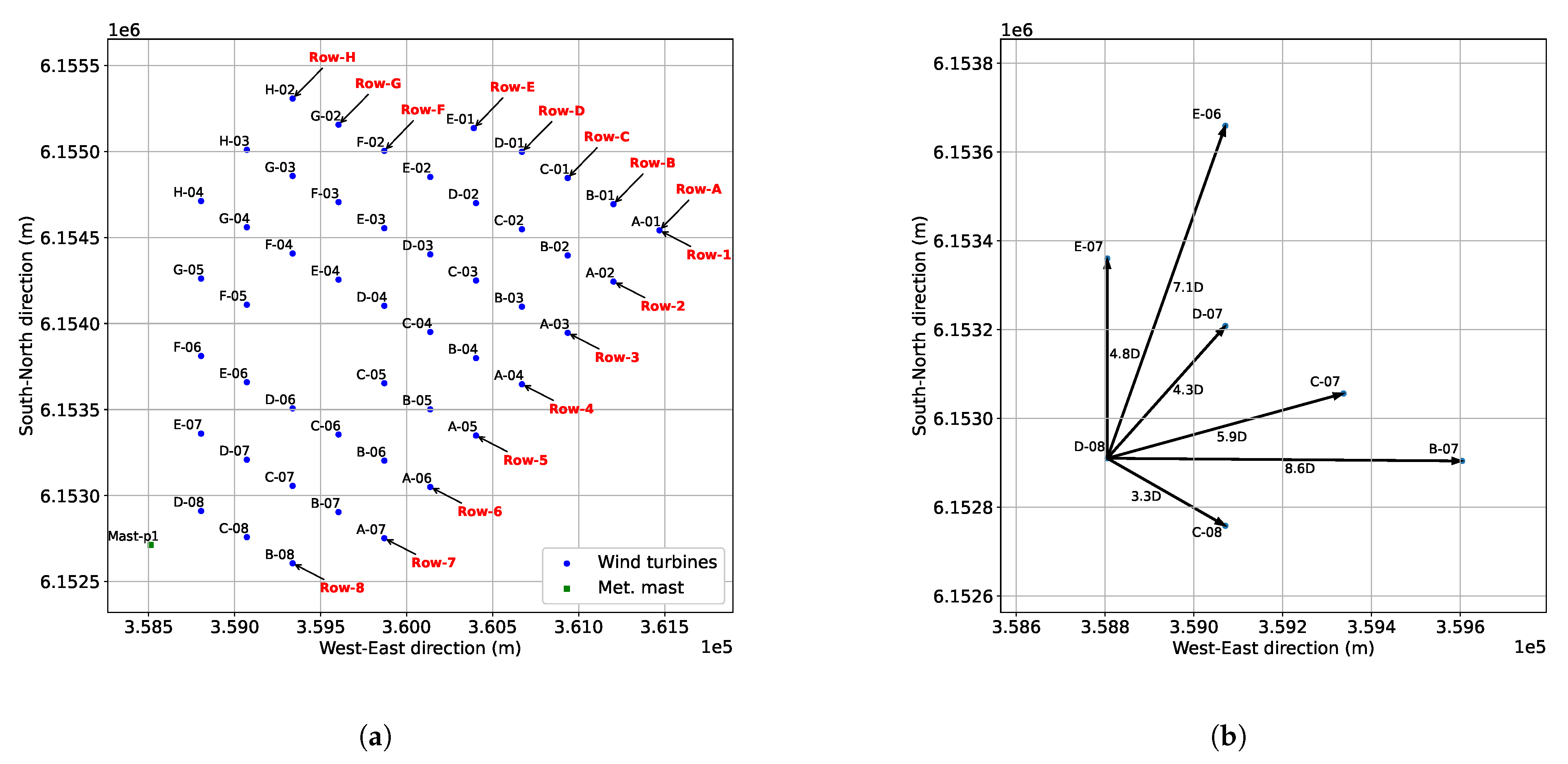
The analysis is performed on the Lillgrund wind farm, which contains 48 Siemens SWT-2.3-93 turbines [42]. The turbines have a rotor diameter of D = 92.6 m, a hub height of 65 m, and a rated power of 2.3 MW. The corresponding rated wind speed is around 12 m/s. The wind farm layout is shown in Figure 1a and it can be seen in Figure 1 that the farm is densely packed with the smallest turbine spacing being 3.3D. All aligned wind directions and the corresponding turbine spacings are summarized in Table 1.
The analysis is performed using SCADA data with 10-min statistical values from the 48 turbines, which record electrical power, rotational speed, local wind speed, pitch angle, and nacelle position measurements. The SCADA data measurement campaign was conducted from 1 January 2008 until 31 December 2012. Furthermore, meteorological measurements are used from a nearby meteorological mast.
The SCADA data is carefully prepared to ensure the validity of the used measurements by removing unrealistic values from the data set. Examples of unrealistic values are wind speeds above 50 m/s and pitch angles larger than 90°. Additional outliers are identified and removed using the Local Outlier Factor (LOF) method [43]. The LOF algorithm computes a score that indicates the abnormality of observations based on the neighboring observations. The score indicates the local density deviation of a given data point with respect to its neighbors. Removing outliers and filtering out unrealistic values yields a data set that mainly contains valid and useful data points, which capture the general behavior including natural variability. After the LOF method is applied and the data is filtered, a total of 4,592,626 10-min average power measurements are left for 48 turbines, equaling approximately 95,680 timesteps or 1.8 years.
The standard deviation of the wind speed, needed to calculate the Turbulence Intensity (TI) of the free stream flow, is only known for measurements from the nearby meteorological masts of which most time steps do not match the ones from the SCADA data measurement campaign. To be able to estimate the TI for all time steps, the meteorological mast data is mapped on the wind direction and wind speed with a bin width of 5° and 0.5 m/s, respectively. Furthermore, a map is created for every season to capture seasonal changes. The maps are not shown for brevity, but two trends can be distinguished. The TIs are the highest in the winter and the lowest in spring. Furthermore, the TIs are generally higher for north-eastern and eastern winds, somewhat lower for southern winds, and again slightly higher for western and north-western winds. This can be explained by the geographical location of the wind farm. The land that is closest to the farm is located to the east and north-west of the farm. Wind over land generally has a higher TI than wind over sea due to the roughness length of the surface.
2.2. FLORIS Model
The FLORIS model (version 2.0.1) [33] has several engineering models available. For this study, a variant of the Gaussian wake model, called the Gauss–Curl Hybrid (GCH) model, is used. The GCH model is comprised of four main elements: the near-wake region, the 2D Gaussian shape of the velocity deficit in the far-wake region, the deflection of the wake centerline, and the secondary wake effects. The GCH model uses a single wake model for wake redirection based on the paper by Bastankhah and Porté-Agel [44]. The model further uses a turbine induced turbulence model [45] and a turbulence summation model [46]. Finally, secondary wake steering is included based on the paper of King et al. [47]. The GCH model parameters will be introduced later in this section and eventually calibrated to the measurements.
2.2.1. Near Wake
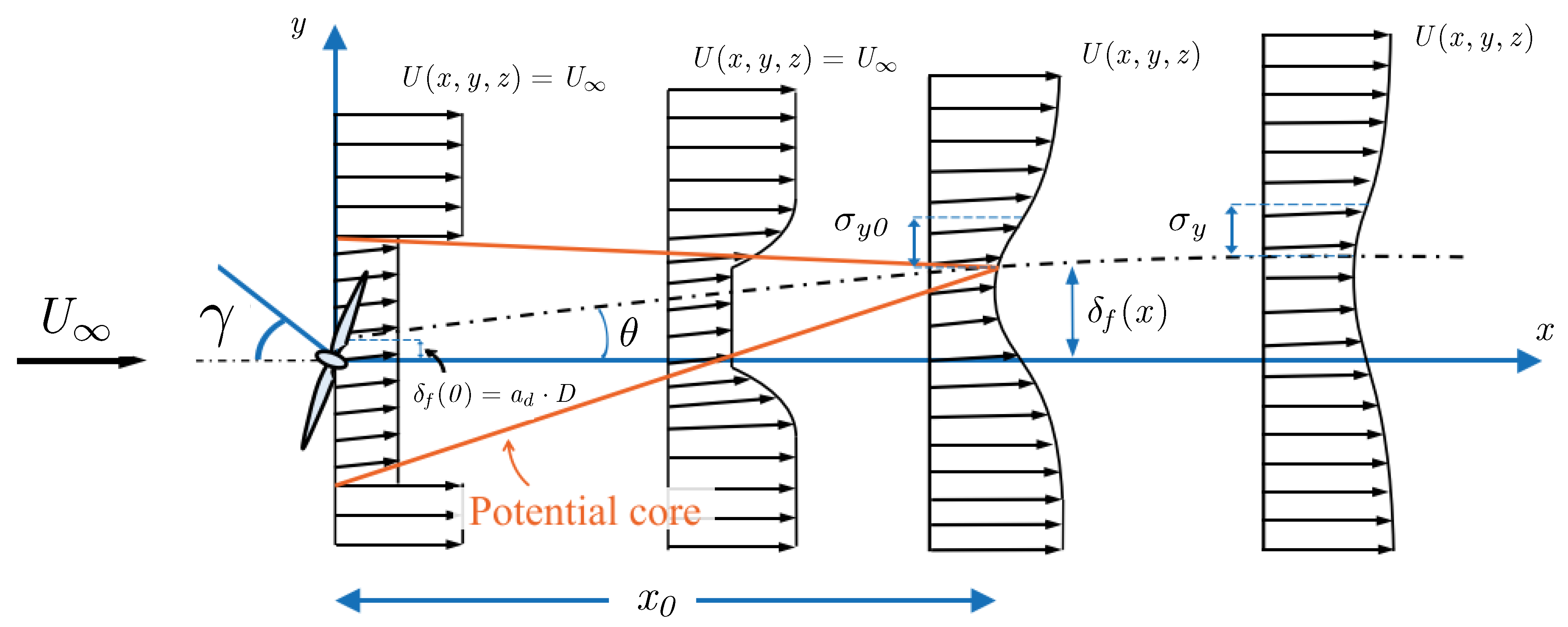
The velocity deficit does not follow a 2D Gaussian distribution in the near wake. The near-wake region is modeled as a linearly converging cone. The base of the cone is located at the rotor, and the tip is located at a distance downstream. This cone is visualized in Figure 2 and is computed as
In Equation (1), is the yaw misalignment angle with the incoming flow in radians, is the thrust coefficient of the rotor, is the TI at the rotor of the turbine. and are the first two model parameters, which governs the influence of turbulence and thrust coefficient on the location of the end of the near wake, respectively.
2.2.2. Velocity Deficit and Wake Deflection
The far-wake region starts at a distance downstream from the turbine. It is assumed that the wake velocity deficit has the shape of a 2D Gaussian distribution from this point onwards until the wake is fully recovered. The wake velocity deficit is expressed as
with the distance given by -4.6cm0cm
and the initial deflection angle defined as
In Equation (2), is the standard deviation in the specified direction (x, y, z) in the Euclidean space. This standard deviation defines the width of the Gaussian-shaped wake deficit.
The Gaussian-shaped wake deficit is centered around the centerline of the wake. This centerline is displaced with a distance in the y-direction from the x-axis as indicated in Figure 2. This displacement occurs due to yaw misalignment and wake rotation and can be calculated with Equation (3), where is the initial deflection angle and can be calculated using Equation (4). Note, that is in radians and defined in FLORIS as positive counter-clockwise relative to the wind direction (in top view), hence Figure 2 illustrates a situation with negative yaw misalignment.
Furthermore, is the velocity deficit at the start of the far-wake region defined in Equation (5) and is defined as Equation (6), while and are defined in Equations (7) and (8), respectively. The coefficients and are linear wake expansion coefficients, which governs the wake recovery, similar to the entrainment constant defined by Jensen [48]. The wake recovery is dependent on as shown by Pena Diaz et al. [49], and hence and are computed using two additional model parameters, namely and , which gives weight to the influence of the turbulence intensity () and the fundamental wake recovery () as seen in Equation (9). Finally, represents an additional wake deflection induced by the rotation of the wake [37] and determined by the linear function shown in Equation (10), which depends on rotor size (D) and downstream distance (x) and the associated two model parameters and , respectively.
2.2.3. Secondary Wake Effects
The Gaussian wake model is transformed into the GCH model through the secondary wake effects. The details of this sub-model can be found in the paper of [47], but the main principles and equations are described here. The model consists of two vortex systems. One is a result of the wake rotation, while the other is a result of the yaw misalignment and is called the counter-rotating vortex [44].
The circulation strength corresponding to these vortices can be used to find the spanwise V and vertical W velocity components based on the wake rotation and yaw misalignment angle anywhere in the space domain. The parameter is introduced in the calculation of the velocity components, which represents the size of the vortex core. In this study, it is assumed that , as it is the standard value in the FLORIS model. The additional wake recovery is defined as
2.3. Calibration Method
The FLORIS model is an engineering model constructed based on simplified physics, and which requires calibration. However, the input power curve provided to FLORIS is crucial in getting a realistic output, and an empirical power curve is therefore derived initially before calibrating the model parameters. Once FLORIS has calculated the local wind speed for every turbine, it should also accurately calculate the power using the empirical power curve and the power-yaw loss coefficient through
where is the yaw misalignment angle and the power from the power curve for local wind speed U.
The empirical power curve is derived using bin averaged SCADA data from free standing turbines at the edge of the farm to exclude wake effects. It should be noted that the epistemic uncertainty in the SCADA data related to measurement uncertainty is essentially unknown and therefore not included in the subsequent calibration. An empirical power curve should reduce the effects on input uncertainty because it encompasses similar uncertainties of wind speed and wind direction measurements as will be used in the calibration. Excluding the input uncertainty from the calibration can have significant effects on the obtained model parameters, because it leads to an increased overestimation in uncertainty of the outputs, which lead to larger uncertainty of the model parameters, see Murcia Leon [50].
The power-yaw loss coefficient is implemented as suggested by the paper of Liew et al. [51]. This paper describes how should be adjusted based on whether a turbine is in the wake of another turbine and what the spacing is between those two turbines. Since the turbine used by Liew et al. [51] has similar characteristics as the Siemens SW-2.3-93 turbine, the values from that paper are directly used in this study. Note, that a different is used per turbine spacing.
Previous model calibrations performed by for instance Fleming et al. [52], Doekemeijer et al. [14], Doekemeijer et al. [40], and Gebraad et al. [37] relied on high-fidelity flow model which was not available in the measured data. Instead, the calibration is set up to minimize the difference between the FLORIS power output and SCADA power measurements by adjusting the model parameters, similar to Göçmen and Giebel [53]. Here, the focus is only on the model parameters related to the Gaussian wake model, i.e., the following model parameters will be calibrated . The optimization used to find the model parameters is defined as
where , n indicating the number of turbines considered, and i corresponds to a combination of wind speed and wind direction , and hence, also turbine spacing.
The calibration is performed using Differential Evolution [54], which yields the global minimum of a multivariate function within defined boundaries. These boundaries are obtained from Doekemeijer et al. [40]. The boundaries for and from Doekemeijer et al. [40] are adjusted to match the Python version of FLORIS. Furthermore, the lower boundary of is changed from −0.01 to 0.0. The boundaries used here are listed in Table 2.
2.4. Yaw Optimization
FLORIS is calibrated for normal operating conditions and subsequently used to determine optimal yaw angles aimed at optimizing the power output and hence AEP. The potential improvements will be compared to a baseline scenario, where all turbines have a zero yaw angle and are thus aligned with the main wind direction. The yaw angles of the turbines will be optimized in two ways, namely deterministic, where input uncertainty is neglected, and robust, where input uncertainties are considered.
2.4.1. Deterministic Optimization
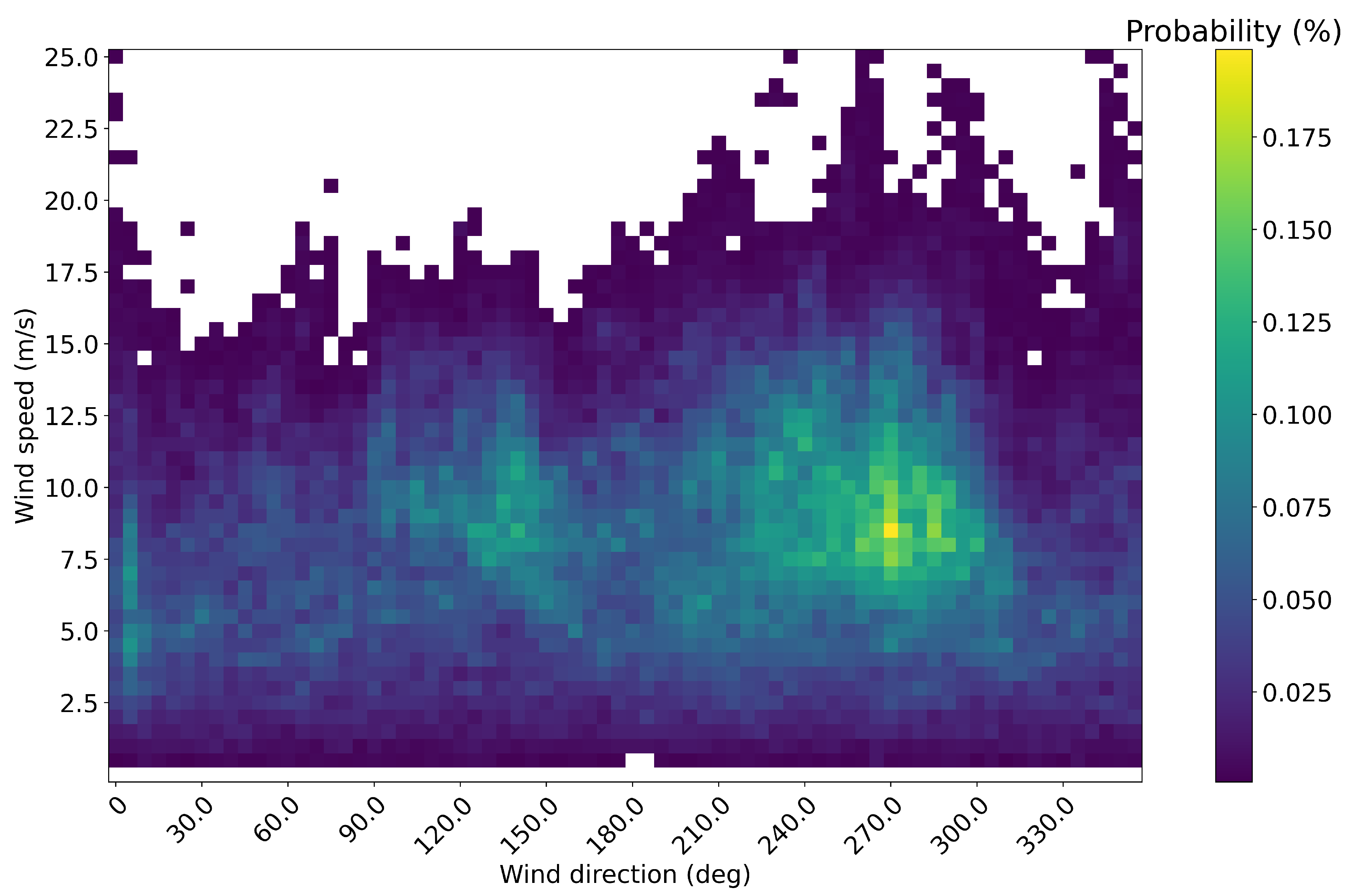
There are a total of 48 variables to optimize, as the yaw angle of each of the turbines is the only control parameter. The cost function used in the minimization is the negative wind farm power and the optimization tool uses a sequential least squares programming algorithm. The aim is to increase the AEP, and hence the optimization is performed for a full wind rose. The wind rose is obtained from data of meteorological mast 1, which conducted a measurement campaign of 2.5 years before the construction of the wind farm. The wind rose is discretized for m/s and and is visualized in Figure 3.
The measurements from the meteorological mast include measurement uncertainty, but as previously described, the influence is reduced by using an empirical power curve, which includes the same uncertainty in wind direction and wind speed.
The deterministic yaw angle sets are indicated as . Once the optimal yaw angles are determined for the full wind rose, the AEP can be calculated for the baseline and optimized case as
where T is the number of hours in a year, is the probability that a specific combination of wind speed and direction occurs, and is the power corresponding to that combination of wind speed and direction. Note, that the subscript k indicates whether it is the baseline or the optimized case. In order to better quantify the difference between baseline and optimized case, the AEP gain is used instead of the AEP alone. The AEP gain is defined as
2.4.2. Optimization under Uncertainty
The optimization can be made more robust by taking the associated uncertainty in wind direction and yaw position into account, i.e., performing Optimization Under Uncertainty (OUU) [16,17,18,55]. The present study is limited to these uncertainties, but many additional input uncertainties can be taken into account, such as uncertainties in wind speed, TI, and wind shear. Following the study of Simley et al. [18], the input uncertainties are related and derived as
In [18], it is also shown that and yields the best fit for . It should be mentioned that the use of these standard deviations for all inflow conditions and turbines is a significant simplification. The robust optimization, which takes the input uncertainties into account, will be denoted , and the deterministic input case will be denoted . It is assumed that two representative normal distributed Probability Density Functions (PDFs) can be obtained using those standard deviations, i.e.,
The PDFs indicate the probability of a deviation from the mean . The subscript i indicates either the wind direction or the yaw position in both and . The PDFs are used to obtain a weighted average of the wind farm power for combinations of wind direction and yaw position errors. The weighted average of power as defined by Simley et al. [18] is
where the superscript j denotes the turbine number. Note, that represents the joint probability distribution of wind direction and yaw position. The joint probability distribution derivation can be found in the paper of Simley et al. [18]. Equation (18) is implemented by approximating the integration as a double summation and by discretizing the wind direction and yaw position. Once calculated, can be used to obtain the robust AEP through Equation (14) by replacing P.
Determining the weighted average of the farm power takes longer than when the farm power is calculated using the deterministic approach because the model needs to be evaluated multiple times with different combinations of wind directions and yaw positions. The number of evaluations N needed for each depends on the number of discretization points of the wind direction PDF and yaw position PDF , through
A convergence study is done to determine the number of evenly spaced steps needed per PDF, to ensure that the weighted average calculation is as fast as possible, without losing too much accuracy. It is found that generally convergence is reached for and , which is similar to what is used by Doekemeijer et al. [14]. The robust yaw angle sets are indicated as .
3. Results
3.1. Sobol Method
The current model setup of FLORIS contains a total of six model parameters, which all affect the accuracy of the model results, but the influence differ for each parameter. Therefore, it is important to examine and quantify the influence of each parameter through a sensitivity analysis. This is done using the variance-based Sobol method [56,57] which is a global and model-independent sensitivity analysis method based on variance decomposition. It can handle non-linear and non-monotonic functions and models. The method decomposes the variance of the model output into fractions that can be connected to parameters or sets of parameters in the model. Hence, the method makes it possible to distinguish highly influential parameters from non-influential parameters.
For full details on the variance-based Sobol method, the reader is encouraged to read the paper of Sobol [56,57] with examples on how to apply the Sobol method by Nossent et al. [58] and Zhang et al. [59]. The Sobol sensitivity indices are characterized by the ratio of the partial variance of the output to the total variance. The model output used for this method is the AEP, meaning that all wind speeds and wind directions are taken into account. The method depends on the choice of distribution and boundaries for each of the evaluated parameters. Uniform distributions have been used, and the boundaries for the model parameters are the same as used in Section 2.3 and shown in Table 2. Note, that the boundary values influence the Sobol index of the parameter, as a larger range for a given parameter will likely yield a higher Sobol index. In this paper, only the first-order sensitivity and the total-order sensitivity are considered, where is a measure of the contribution of the individual parameter to the total model variance, and describes the main effect of and all its interactions with other parameters. In other words, one can determine the impact of the interaction between and other parameters by analyzing the difference between and .
The reliability of the Sobol indices can be tested by using confidence intervals. Bootstrapping with re-sampling is used to obtain 100 samples from the model output distribution [60] and hence distributions of and . The 95% confidence intervals can be determined from these distributions. In general, the confidence intervals of the most sensitive parameters should be as small as possible, and ideally smaller than 10% of the sensitivity indices for the most sensitive parameters [59]. If the confidence intervals are larger than 10%, it means that the Sobol indices are not fully converged yet and that the model should be evaluated more times. For the indices shown, the model has been evaluated 12,000 times.
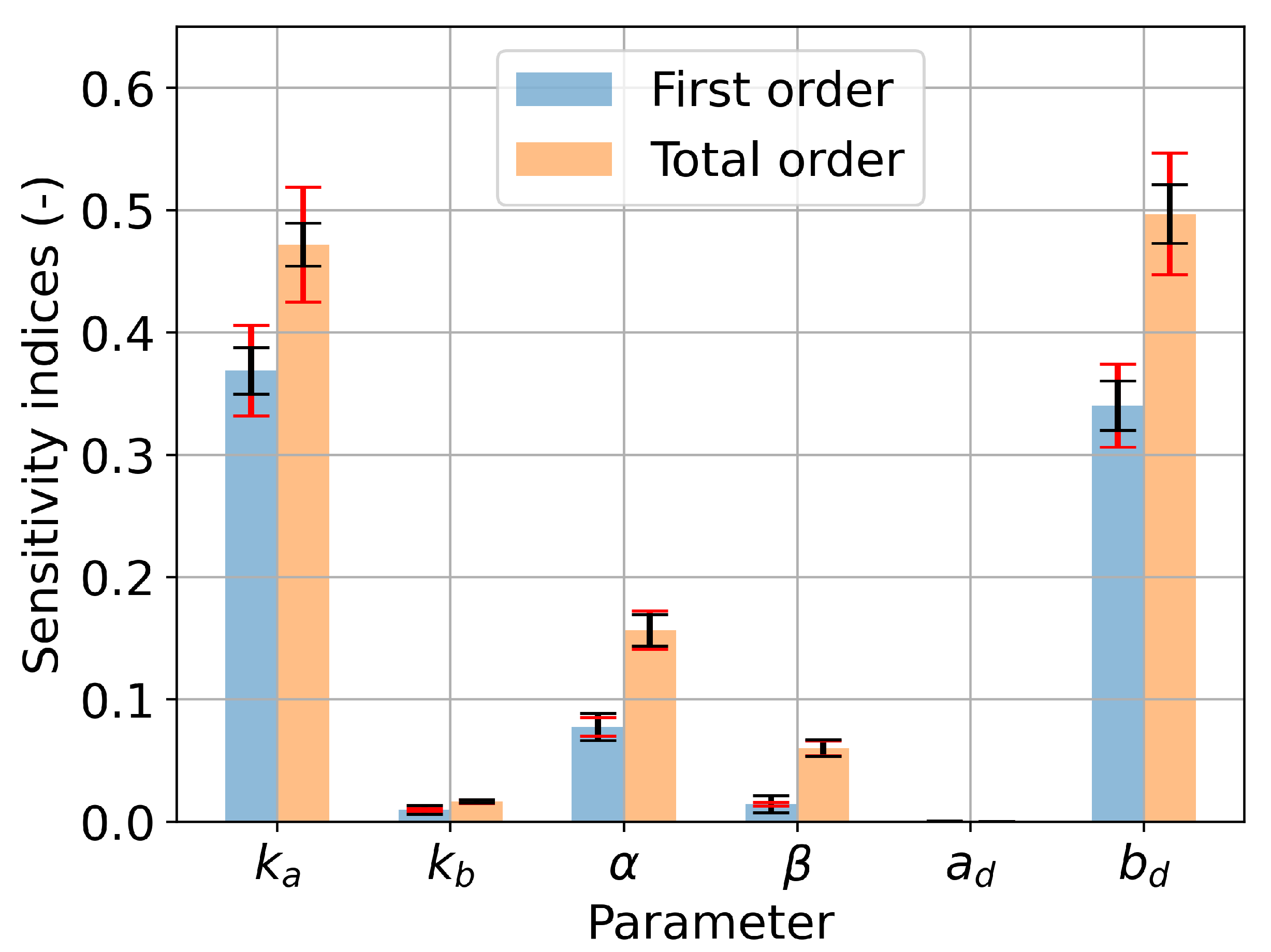
The first and total-order sensitivity indices for a turbine spacing of 4.8D are shown in Figure 4. The confidence intervals are shown in black and the 10% intervals in red. First of all, the figure shows that the confidence intervals of the most sensitive parameters are within, or very close to, the 10% deviation. Furthermore, it can be seen that only three model parameters have a significant effect on the model output variance, namely , , and to some degree . In total these three parameters account for approximately 79% of the model output variance. This means that the three sub-models, describing the near-wake region, wake deflection, and velocity deficit, all influence the output significantly. However, the insignificant effects of some of the model parameters indicate that certain sub-models or the combined model complex might be overparameterized. The effect of is negligible, hence this parameter is set to zero, every time the model is used. Finally, for all parameters, the total-order sensitivity is significantly higher than the first-order sensitivity. This indicates that there are some significant second-order (and probably higher-order) sensitivities, meaning that there is significant parameter interaction.
The Sobol indices for all main directions and the associated spacings are presented in Figure 5. Figure 5 shows that the parameters are generally converged with the 95% confidence intervals being within the 10% deviation, except for and for the largest two spacings. This again implies that the estimations of the Sobol indices are not fully converged for these two parameters. However, the results still indicate the parameters’ dependence in relation to the turbine spacing. The changing sensitivity of the model parameters for each turbine spacing highlights the need to map the model parameters for each turbine spacing during the calibration, which is done in Section 3.2. Additionally, the negative values for are non-physical but occur because the Sobol method is not fully converged, and since the Sobol index of is close to zero.
The three most sensitive parameters have different trends for varying turbine spacing. It can be seen that the sensitivity of increases as the turbine spacing increase. The sensitivity of and follow the opposite trend; they are higher for relative short turbine spacings and lower for larger turbine spacings. These changes in sensitivity are expected because influences the near-wake, which is less influential for larger spacings. The lateral deflection influenced by Equation (10) is relatively small compared to the lateral deflection described by the other parameters Equation (3) for larger spacings. The observed trends in sensitivities are similar for both the baseline and the optimized scenario.
3.2. Calibration Method
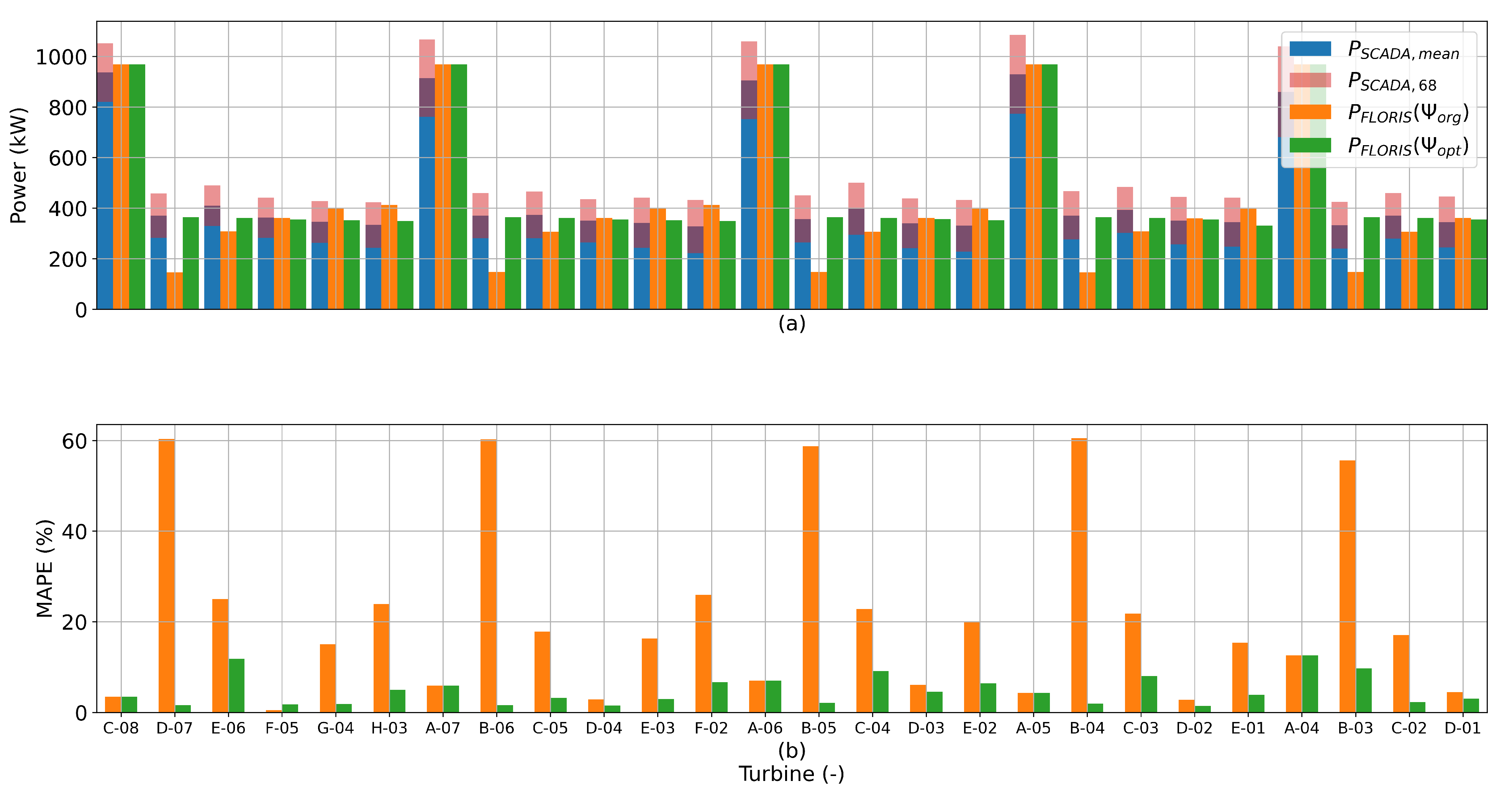
Figure 6 shows the power predictions of FLORIS before and after the calibration compared to the power measurements from the SCADA data for = 8 m/s and , which is a frequently occurring wind combination. The plot shows the output of FLORIS for the standard model parameters and for the optimal model parameters , including the Mean Absolute Percentage Error (MAPE) per turbine. It can be seen that performs much better than and that all predictions of FLORIS using fall within the 68% confidence interval of the SCADA data. The average MAPE of all turbines shown in Figure 6 is minimized to 5.7%.
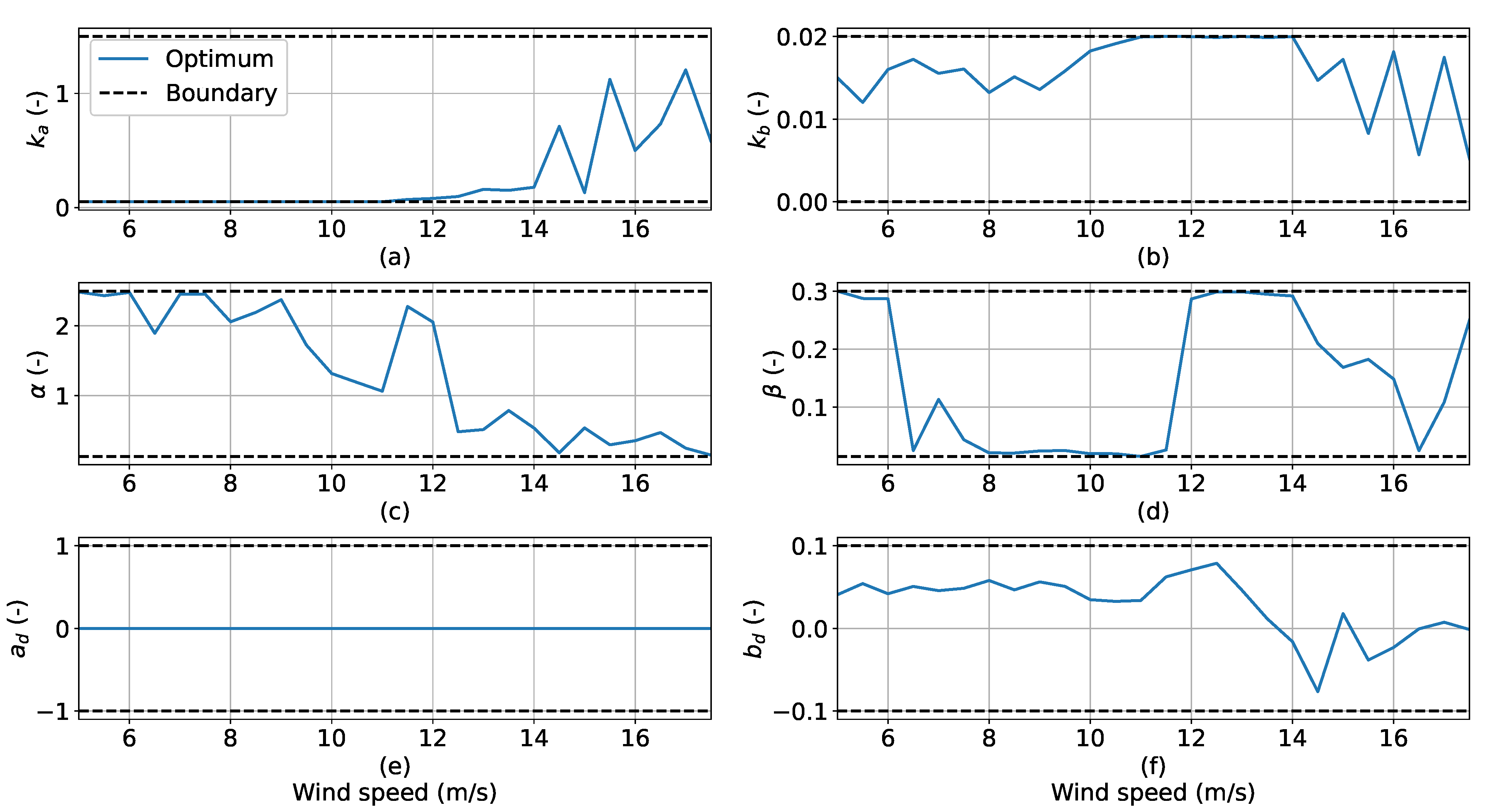
However, the average MAPE increases if is applied for other wind speeds. A new set of model parameters can be found for each wind speed, where A represents the combination = 8 m/s and and B represents for example = 10 m/s and . Hence, the model parameters are wind speed dependent. Therefore, is found for every wind speed independently. Figure 7 shows how the model parameters change for varying wind speed. Generally, the parameter values are spread over the entire domain, except for and . It can also be seen that is often close to its lower boundary and that is closer to the upper boundary. However, it should be noted that the sensitivity of is relatively low, as discussed in Section 3.1. Hence, is still the dominating parameter for the wake expansion. There is also a clear trend that the major change in parameter value occurs as the wind speed increases above rated, where the wake effects are significantly reduced. The model parameters are only obtained for wind speeds from 5 m/s up to 17.5 m/s, since all turbines operate at rated power for higher wind speeds, even at the smallest turbine spacings, and downstream waked turbines do not operate when the upstream turbine experiences wind speeds below 5 m/s.
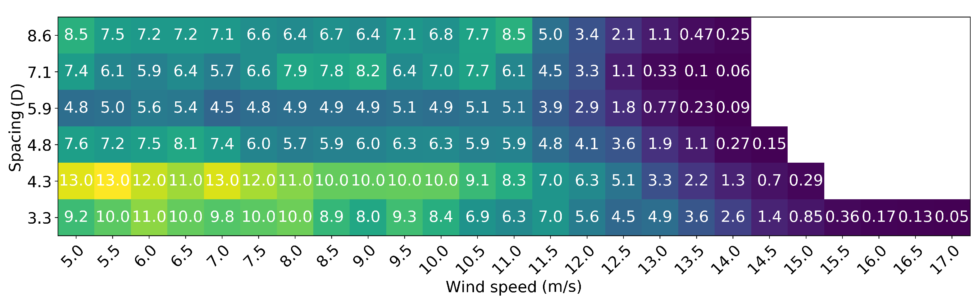
The variation of the six model parameters shown in Figure 7 can also be determined for every turbine spacing. The corresponding average errors of the predicted power production for each wind speed and turbine spacing is shown in Figure 8. The highest MAPEs occur for small turbine spacings and the lowest MAPEs for large turbine spacings. This is expected as the FLORIS model is intended for far-wake modeling. Furthermore, the behavior of the MAPE is the same for every turbine spacing. It is generally the highest for low wind speeds and it decreases slightly with increasing wind speed before it converges to zero as all turbines in the row start to operate at rated power. The standard deviation of the MAPE follows the same trend but is not shown for brevity.
The shown MAPEs are based on the calibrated model parameters for each wind speed and each turbine spacing. The MAPE will increase significantly if the model parameters of the case with a spacing of 3.3D are applied on another spacing, e.g., 5.9D. Hence, all model parameters need to be calibrated as a function of wind speed and turbine spacing instead of a single constant value in order to achieve accurate model predictions. These dependencies might also depend on additional conditions, such as atmospheric stability.
3.3. Model Uncertainty
The model bias and uncertainty can be quantified using the SCADA data as a benchmark. The method used is proposed and fully described by Nygaard [61]. The main principle is to estimate the discrepancy distribution between measured data and the model output. The mean of this distribution gives the bias of the model and the width of the distribution gives an estimation of the uncertainty. The method relies on the power output as a function of inflow wind speed and wind direction only. The benchmark of the model is the wake loss defined as
The angle brackets 〈..〉 denote the mean value of the validation sample considered. This validation sample is derived from the available SCADA data. The subscript i indicates the case, i.e., either the observed case using measured values or the model case . The gross power is the power estimation produced by the farm with no wake effects, and the net power is the power estimation of the wind farm including wake effects. The wake losses can be used to find the relative wake model error defined as
The model underestimates the wake losses for , i.e., the estimated AEP is optimistic. By contrast, the estimated AEP is conservative when .
A statistical re-sampling approach, called the circular block bootstrap method [62], is used to get a distribution of the relative wake model error. This method divides the validation sample, which essentially is a time series of SCADA data, into overlapping blocks of length k and wraps the time series to connect the beginning and the end. The created blocks are then randomly sampled with replacement until a new unique time series is created with the same size as the original validation sample. This unique time series is then one bootstrap sample of which , and can be derived. This process is repeated N times to get a distribution of .
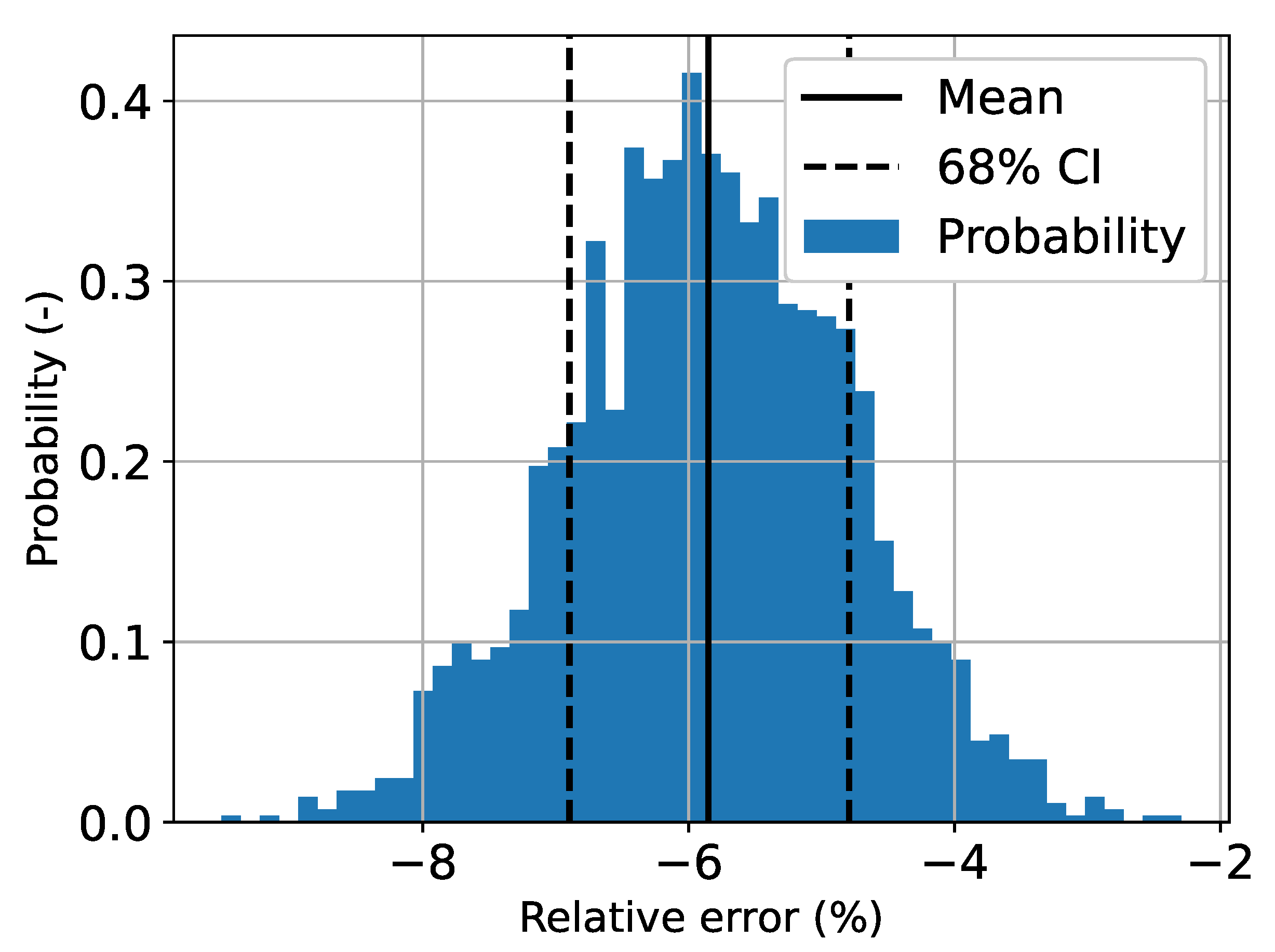
The method is applied with time steps and samples. The high value of N is chosen to obtain a smooth distribution, but the sample size does not affect the resulting bias and uncertainty from N = 500 onwards. The corresponding relative wake model error distribution is shown in Figure 9. The mean value, hence the bias, is −5.8%, meaning that the model estimate tends to be conservative. The uncertainty, as mentioned before, is defined as the half-width of the 68% confidence interval. In this case, the model uncertainty is ±1.1%. Although there is a significant bias, the FLORIS model is still able to estimate the wake loss with low uncertainty. This model uncertainty means a wake loss of 30% essentially has a 68% confidence interval of (29.7%, 30.3%). However, this does not include the determined bias, which corrects the predicted wake loss with a 68% confidence interval to (27.9%, 28.6%).
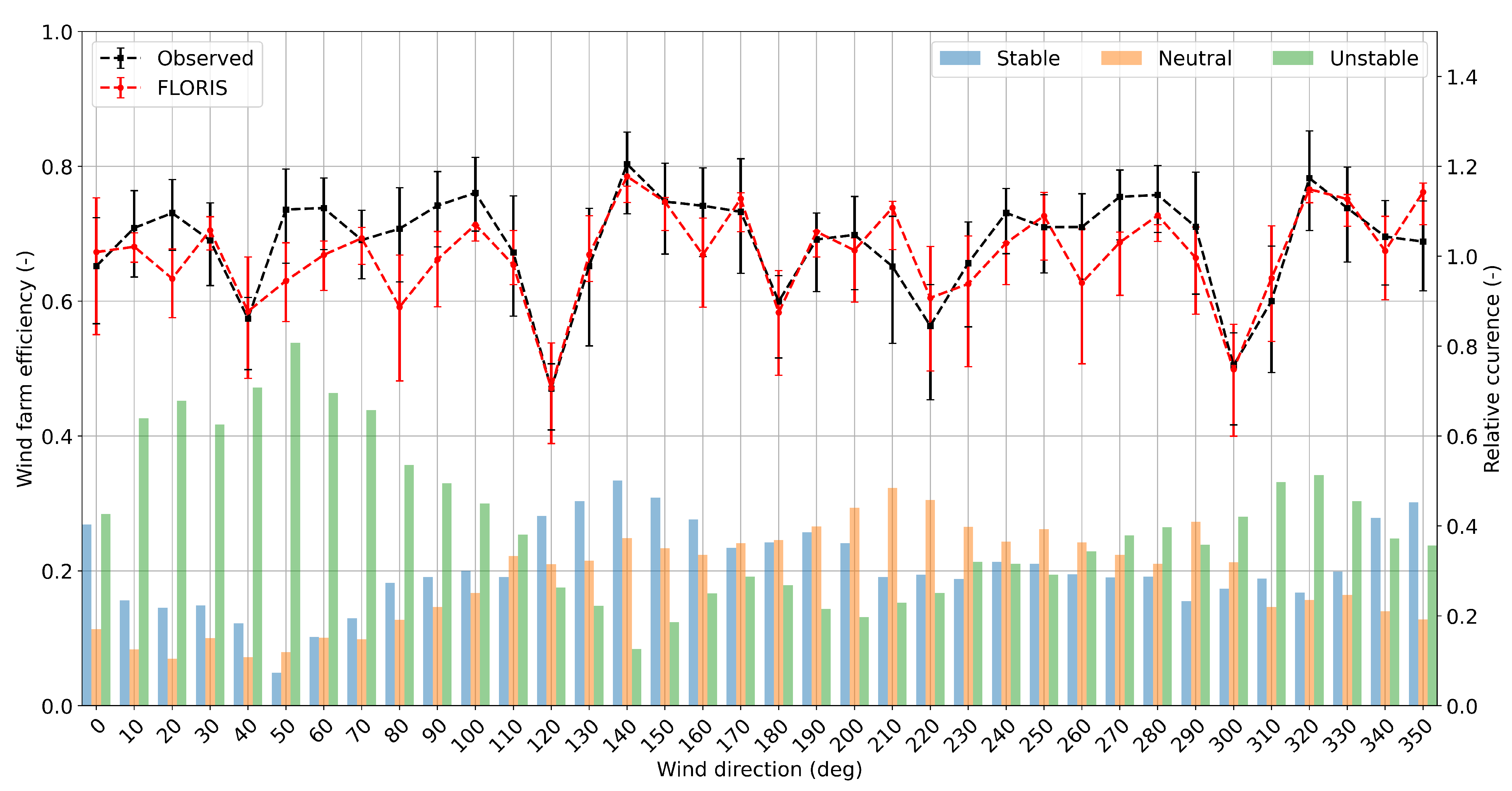
The wind farm efficiency can be calculated through
where the subscript d denotes the wind direction bin and the angle brackets indicate the mean value of the power measurements of all timesteps for a given wind direction measurement in d. Note, that the wind farm efficiency is the same as one minus the wake loss. The wind farm efficiency is plotted for different wind directions in Figure 10. It is seen that the FLORIS model output follows the general trends and matches most peaks and troughs of the observed data, except for two turbine spacings, namely 5.9D (75° & 255°) and 8.6D (90° & 270°). The wake loss is especially overestimated by the FLORIS model in the 10–110° sector. The error bars show the 25th and 75th quartiles of the observed and modeled values, and hence show the width of the distributions. Generally, the two distributions overlap, particularly where the model performs well, which indicates that results are statistically comparable and the variation in the model input does to some degree capture part of the variability seen in the observations. However, the modeled distribution frequently appears more skewed than the observed values, e.g., 50–70° and 130–220°, while the observed distributions appear more symmetric.
The discrepancy between the observed and modeled efficiencies can potentially be attributed to the influence of the atmospheric stability. The atmospheric stability was previously estimated for the Lillgrund wind farm from the nearby Drogden light tower for the period of 2008–2013 by Larsen et al. [63] and has been categorized as either stable, neutral, or unstable based on the Monin–Obukhov length [64,65]. However, it has not been possible to directly link all the stability measurements with the SCADA data, but the stability classification is shown as a function of wind direction in Figure 10 to visualize the correlation between the atmospheric stability and the ability of the FLORIS model to predict the wake loss accurately. The stability is predominantly unstable for eastern winds and north-western winds. This is presumably because the winds during autumn and winter are often cold winds coming from land, which can result in an unstable atmosphere when it is traveling over a relatively warmer surface as the sea, which is not fully cooled down yet.
The FLORIS model mainly overestimates the wake loss in the 10–110° wind direction sector, where the atmosphere is predominantly unstable. The analysis suggests that the FLORIS model with the current wind shear setting is, in general, better able to model stable and neutral atmospheric conditions compared to unstable atmospheric conditions. This highlights the importance of taking into account the atmospheric stability. Atmospheric stability effects can potentially be included by adjusting the wind shear accordingly and to include the separate effect on changing TI [66]. However, such adjustments are not applied in this study, because adjusting the TI and wind shear based on the stability would require additional assumptions and hence additional uncertainties.
3.4. Yaw Optimization
Section 2.4 described how the optimized yaw angle sets and can be derived. The performance of each yaw angle set is tested for three input cases, which are summarized in Table 3. The first column of Table 3 shows the three input cases. Note, that an additional input case is introduced which is used to test the robustness of the yaw angle sets since both yaw sets are not optimized for this input case. The second column shows the input uncertainty for each case given as a standard deviation of a normal distribution. The third column shows the potential AEP gain for each input case for the optimized yaw set determined using input case . Finally, the fourth column shows the potential AEP gain per input case for the optimized yaw set determined using input case .
The highest AEP gain of 6.1% can be observed for the deterministic yaw set and deterministic input case . Assuming the same model uncertainty for the optimized case as for the baseline case yields a 68% confidence interval of the energy gain as (5.5%, 6.6%). Furthermore, it is also assumed that the model bias is the same for the baseline and optimized case, i.e., bias influences both and in Equation (15) in the same way, and therefore, the model bias does not influence the estimated relative energy gain.
The energy gain for the more robust yaw set and deterministic input case is 2.5% with a 68% confidence interval of (1.8%, 3.1%), which is significantly lower than the 6.1% observed for . The deterministic input case assumes perfect knowledge of the wind direction and yaw position, which is usually not the case. Higher gains are observed for input cases and when input uncertainties are included in the yaw optimization (). For example, the energy gain for input case increases from 2.5% to 3.4%, which is an increase of 36%. On the other hand, a lower gain can be observed for input case .
The yaw set also performs better for the larger input uncertainty case . Thus, can be considered to be more robust than . The most realistic input uncertainty of the cases considered is presumably . The final estimation of the potential AEP gain for the Lillgrund wind farm is, therefore, 3.4% with a 68% confidence interval of (2.8%, 4.0%) using , which is in the same order as the 3.7% found by Gebraad et al. [38] for the Princess Amalia Wind Park in the Netherlands.
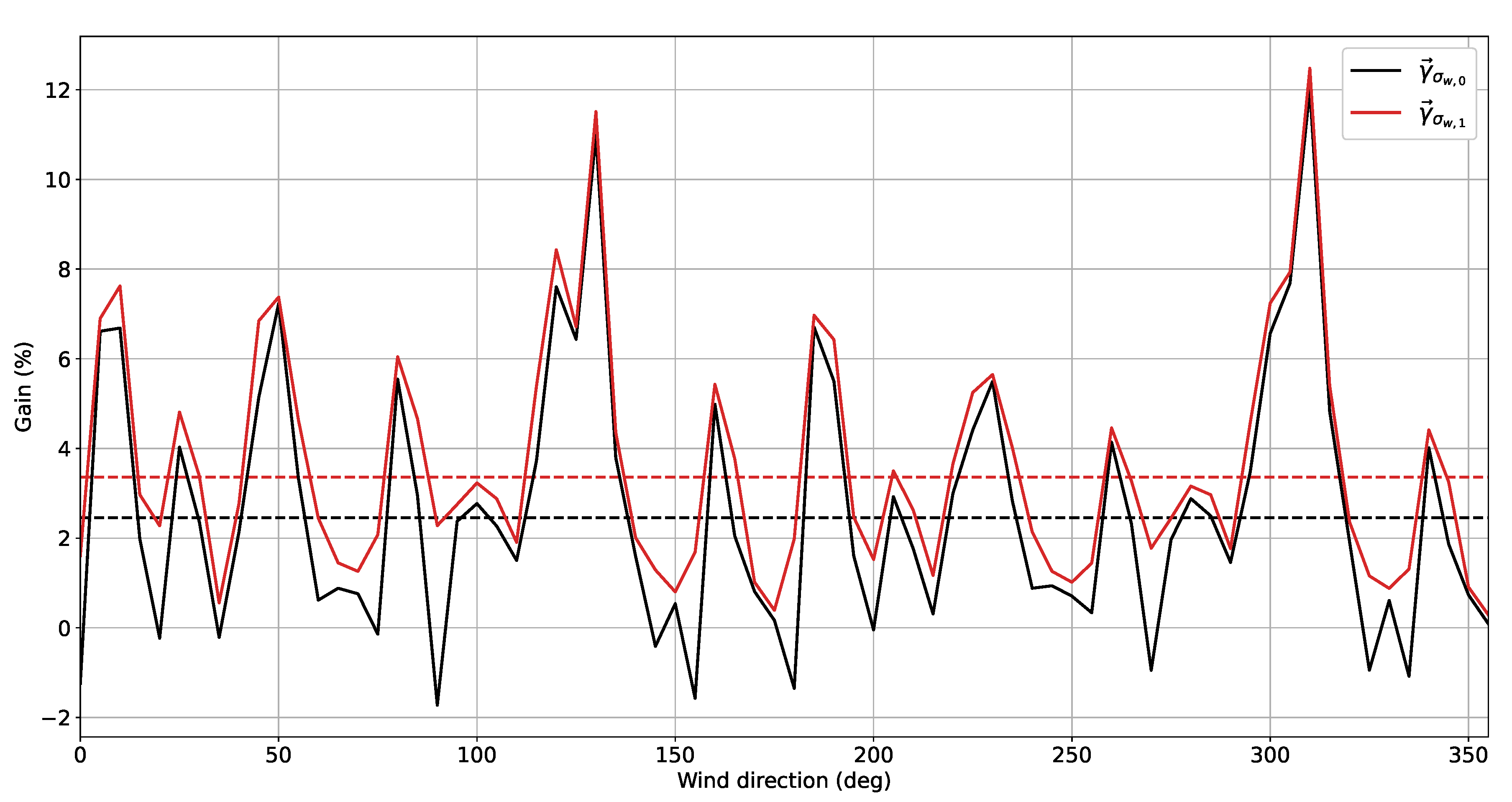
In order to identify for which wind directions the energy gain is achieved, and what the differences are between the gains of yaw angle sets and , the gains are plotted as a function of wind direction in Figure 11 for input case . It is seen how occasionally yields locally negative gains, while constantly shows positive gains. The largest differences between the two curves are observed for alignment directions (90°, 155°, 180°, etc.).
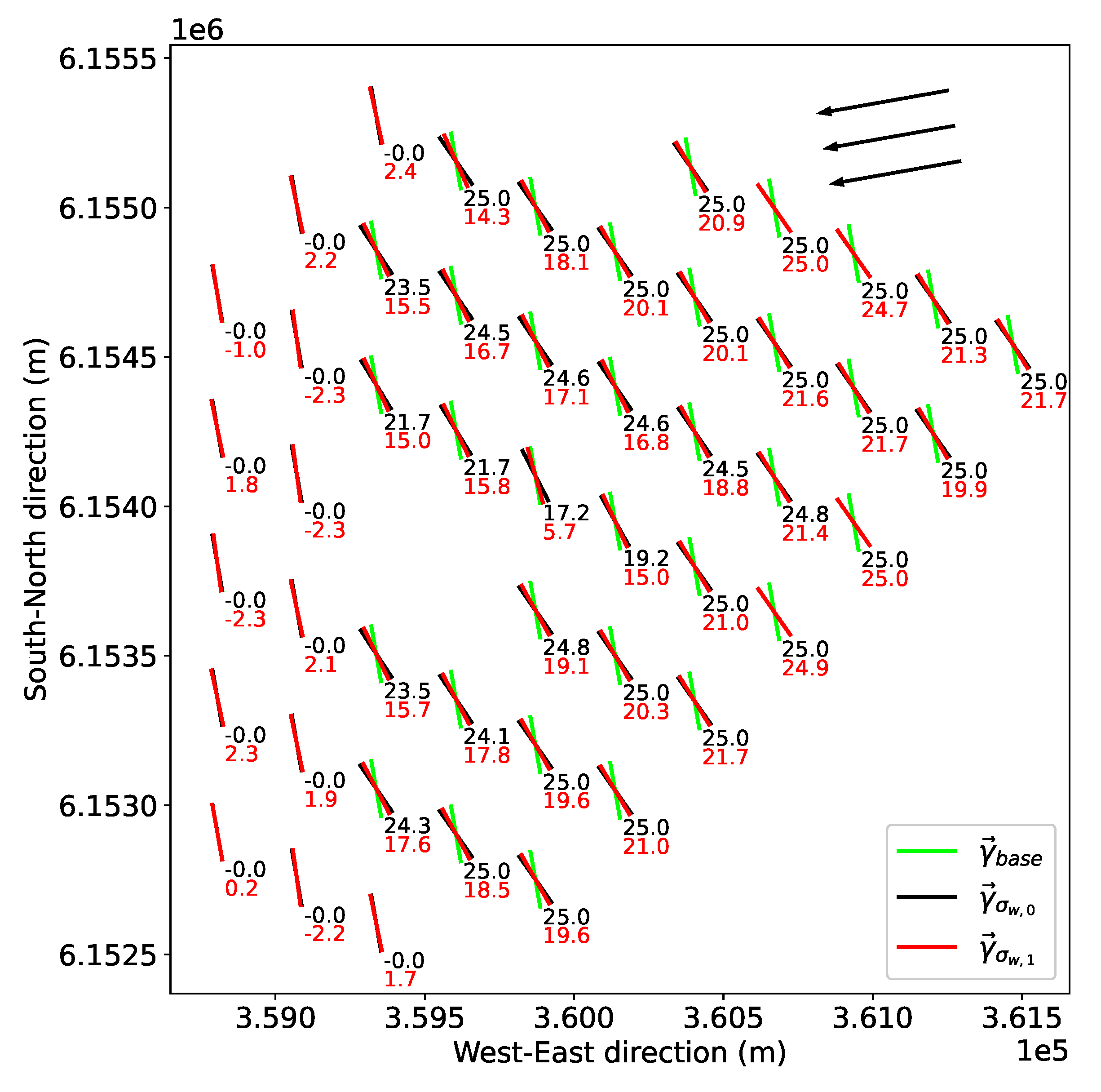
Figure 12 shows the yaw angle sets for the three different scenarios for a wind direction of 80° and a wind speed of 8 m/s. The more robust yaw angle set (lower number in red) is compared with the deterministic yaw angle set (upper number in black). In general, it can be seen that the robust yaw angles are smaller than the deterministic ones. This is an expected consequence of including uncertainty of yaw and wind direction because the sensitivity of power is higher for larger yaw angles and the optimization does therefore result in smaller yaw angles, which are more robust against changing wind directions.
Similar behavior is observed by Rott et al. [17], who also shows that more robust yaw angles result in a lower yaw activity, which is beneficial especially for the turbine control. Furthermore, it is evident how the most downstream turbines generally have a slightly larger yaw angle for . This is again because the turbines prefer to align themselves for the combination of yaw and wind direction deviations with fewer wake effects, in order to increase the power produced in these situations [17].
4. Conclusions
Wake effects impact the aerodynamic performance of large wind farms, which results in decreased power production of wind turbines operating in clusters as opposed to free-standing turbines. This work uses the wind farm model FLORIS to estimate the potential of reducing wake losses by applying yaw-based wake steering. The Lillgrund wind farm is used as a test case. The methodology is divided into three steps: model calibration, sensitivity study, and optimization including uncertainty.
Firstly, a global sensitivity analysis was performed to assess the relative effect of the various model parameters. It was found that three model parameters account for approximately 79% of the total model output variance, while the others have a smaller influence, indicating that the model could be over-parameterized.
Secondly, the model parameters were calibrated to match the power production of the Lillgrund wind farm. The calibration clearly showed that the amount of available data and the data quality are important. In particular, the model parameters were dependent on both wind speed and turbine spacing, so their values should be considered carefully. The performance of the calibrated model was tested by comparing wake losses with measured data. Overall, the wake losses were generally overestimated by 5.8% but the model estimates were considered to be reliable with only a 1.1% model uncertainty. It was also found that the model bias correlated with the changes in predominant atmospheric conditions from different wind directions, suggesting that more data on the atmospheric stability would improve the model predictions. Thirdly, FLORIS was used to optimize the individual turbine yaw angles, in order to increase the potential energy gain of the wind farm. Three cases were considered: a deterministic case without uncertainty in the wind direction and yaw settings, and two cases with uncertainty in the wind direction and yaw settings. The potential AEP gain was larger for the deterministic input case (6.1%) compared with the deterministic yaw angle case with input uncertainty (2.5%). The potential energy gain was shown to increase further by including uncertainty in the yaw angles during the optimization procedure. In particular, the AEP gain was increased by 36% when OUU was used for the yaw angles, leading to a more robust yaw angles set. Overall, the observed AEP gain of 3.4% with OUU shows the potential of wake steering as a control strategy to increase the power production of wind farms.
This work was performed in the context of the Lillgrund wind farm, which is very dense compared to modern wind farms. Future work should assess the potential for wake steering when increasing turbine spacing. Furthermore, this work relies on two fundamental assumptions: (i) neglecting the input uncertainty during calibration, and (ii) constant bias and uncertainty for all model applications (i.e., for both yawed and non-yawed cases). These strong assumptions would need to be validated based on long term measurement campaigns. Finally, this paper showed the importance of the amount of available data and the data quality. Additional data on atmospheric stability could refine the present findings.
Author Contributions
Conceptualization and methodology was developed by all authors, while the analysis was performed by M.T.v.B.; First draft was prepared by M.T.v.B., and editing and review by all authors. All authors have read and agreed to the published version of the manuscript.
Funding
This research received no external funding.
Institutional Review Board Statement
Not applicable.
Informed Consent Statement
Informed consent was obtained from all subjects involved in the study.
Data Availability Statement
The authors have signed a Non-Disclosure Agreement regarding the Lillgrund farm database, so the original dataset cannot be shared.
Acknowledgments
The authors would like to thank Bart Doekemeijer, Tuhfe Göçmen, Kurt Schaldemose Hansen and Nikolai Gayle Nygaard for their meaningful insights. Furthermore, we would like to thank Vattenfall for the data set.
Conflicts of Interest
The authors declare no conflict of interest.
Abbreviations
The following abbreviations are used in this manuscript:
| AEP | Annual Energy Production |
| DIC | Dynamic Induction Control |
| DIPC | Dynamic Individual Pitch control |
| DTU | Danmarks Tekniske Universitet |
| FLORIS | FLOw Redirection and Induction in Steady-state |
| GCH | Gauss–Curl Hybrid |
| LOF | Local Outlier Factor |
| MAPE | Mean Absolute Percentage Error |
| OUU | Optimization Under Uncertainty |
| SCADA | Supervisory Control Furthermore, Data Acquisition |
| TI | Turbulence Intensity |
References
- IRENA. Renewable Energy Statistics 2019; IRENA: Abu Dhabi, UAE, 2019. [Google Scholar]
- Barthelmie, R.J.; Hansen, K.S.; Frandsen, S.T.; Rathmann, O.; Schepers, J.G.; Schlez, W.; Phillips, J.; Rados, K.; Zervos, A.; Politis, E.S.; et al. Modelling and measuring flow and wind turbine wakes in large wind farms offshore. Wind Energy 2009, 12, 431–444. [Google Scholar] [CrossRef]
- Lissaman, P.B.S. Energy Effectiveness of Arbitrary Arrays of Wind Turbines. J. Energy 1979, 3, 323–328. [Google Scholar] [CrossRef]
- González, J.S.; Payán, M.B.; Riquelme-Santos, J.M. Optimization of wind farm turbine layout including decision making under risk. IEEE Syst. J. 2012, 6, 94–102. [Google Scholar] [CrossRef]
- Steinbuch, M.; de Boer, W.W.; Bosgra, O.H.; Peters, S.A.W.M.; Ploeg, J. Optimal control of wind power plants. J. Wind. Eng. Ind. Aerodyn. 1988, 27, 237–246. [Google Scholar] [CrossRef]
- Johnson, K.E.; Thomas, N. Wind farm control: Addressing the aerodynamic interaction among wind turbines. In Proceedings of the American Control Conference, St. Louis, MO, USA, 10–12 June 2009; pp. 2104–2109. [Google Scholar]
- Annoni, J.; Gebraad, P.M.O.; Scholbrock, A.K.; Fleming, P.A.; van Wingerden, J.W. Analysis of axial-induction-based wind plant control using an engineering and a high-order wind plant model. Wind Energy 2016, 1135–1150. [Google Scholar] [CrossRef]
- Bossanyi, E.; Ruisi, R. Axial induction controller field test at Sedini wind farm. Wind. Energy Sci. Discuss. 2020, 1–27. [Google Scholar] [CrossRef]
- Fleming, P.A.; Gebraad, P.M.O.; Lee, S.; van Wingerden, J.W.; Johnson, K.E.; Churchfield, M.J.; Michalakes, J.; Spalart, P.; Moriarty, P.J. Simulation comparison of wake mitigation control strategies for a two-turbine case. Wind Energy 2015, 18, 2135–2143. [Google Scholar] [CrossRef]
- Kheirabadi, A.C.; Nagamune, R. A quantitative review of wind farm control with the objective of wind farm power maximization. J. Wind. Eng. Ind. Aerodyn. 2019, 192, 45–73. [Google Scholar] [CrossRef]
- Rodrigues, S.F.; Teixeira Pinto, R.; Soleimanzadeh, M.; Bosman, P.A.N.; Bauer, P. Wake losses optimization of offshore wind farms with moveable floating wind turbines. Energy Convers. Manag. 2015, 89, 933–941. [Google Scholar] [CrossRef] [Green Version]
- Jimenez, A.; Crespo, A.; Migoya, E. Application of a LES technique to characterize the wake deflection of a wind turbine in yaw. Wind Energy 2010, 13, 559–572. [Google Scholar] [CrossRef]
- Wagenaar, J.W.; Machielse, L.A.H.; Schepers, J.G. Controlling wind in ECN’s scaled wind farm. In Proceedings of the European Wind Energy Conference and Exhibition, Copenhagen, Denmark, 16–19 April 2012; pp. 161–168. [Google Scholar]
- Doekemeijer, B.M.; van Wingerden, J.W.; Fleming, P.A. A tutorial on the synthesis and validation of a closed-loop wind farm controller using a steady-state surrogate model. In Proceedings of the American Control Conference, Philadelphia, PA, USA, 10–12 July 2019; pp. 2825–2836. [Google Scholar]
- Gebraad, P.M.O.; Churchfield, M.J.; Fleming, P.A. Incorporating Atmospheric Stability Effects into the FLORIS Engineering Model of Wakes in Wind Farms. J. Phys. Conf. Ser. 2016, 753, 052004. [Google Scholar] [CrossRef] [Green Version]
- Quick, J.; King, J.; King, R.N.; Hamlington, P.E.; Dykes, K. Wake steering optimization under uncertainty. Wind. Energy Sci. Discuss. 2020, 5, 413–426. [Google Scholar] [CrossRef] [Green Version]
- Rott, A.; Doekemeijer, B.M.; Seifert, J.K.; van Wingerden, J.W.; Kühn, M. Robust active wake control in consideration of wind direction variability and uncertainty. Wind. Energy Sci. 2018, 3, 869–882. [Google Scholar] [CrossRef] [Green Version]
- Simley, E.; Fleming, P.A.; King, J. Design and Analysis of a Wake Steering Controller with Wind Direction Variability. Wind. Energy Sci. Discuss. 2020, 5, 451–468. [Google Scholar] [CrossRef] [Green Version]
- Churchfield, M.J.; Lee, S.; Michalakes, J.; Moriarty, P.J. A numerical study of the effects of atmospheric and wake turbulence on wind turbine dynamics. J. Turbul. 2012, 13, N14. [Google Scholar] [CrossRef]
- Fleming, P.A.; Annoni, J.; Churchfield, M.J.; Martínez-Tossas, L.A.; Gruchalla, K.; Lawson, M.; Moriarty, P.J. A simulation study demonstrating the importance of large-scale trailing vortices in wake steering. Wind. Energy Sci. 2018, 3, 243–255. [Google Scholar] [CrossRef] [Green Version]
- Bastankhah, M.; Porté-Agel, F. Wind farm power optimization via yaw angle control: A wind tunnel study. J. Renew. Sustain. Energy 2019, 11, 023301. [Google Scholar] [CrossRef] [Green Version]
- Campagnolo, F.; Petrović, V.; Bottasso, C.L.; Croce, A. Wind tunnel testing of wake control strategies. In Proceedings of the American Control Conference, Boston, MA, USA, 6–8 July 2016; pp. 513–518. [Google Scholar]
- Doekemeijer, B.M.; Kern, S.; Maturu, S.; Kanev, S.; Salbert, B.; Schreiber, J.; Campagnolo, F.; Bottasso, C.L.; Schuler, S.; Wilts, F.; et al. Field experiment for open-loop yaw-based wake steering at a commercial onshore wind farm in Italy. Wind. Energy Sci. Discuss. 2021, 6, 159–176. [Google Scholar] [CrossRef]
- Howland, M.F.; Lele, S.K.; Dabiri, J.O. Wind farm power optimization through wake steering. Proc. Natl. Acad. Sci. USA 2019, 116, 14495–14500. [Google Scholar] [CrossRef] [Green Version]
- Goit, J.P.; Meyers, J. Optimal control of energy extraction in wind-farm boundary layers. J. Fluid Mech. 2015, 768, 5–50. [Google Scholar] [CrossRef] [Green Version]
- Frederik, J.A.; Weber, R.; Cacciola, S.; Campagnolo, F.; Croce, A.; Bottasso, C.L.; van Wingerden, J.W. Periodic dynamic induction control of wind farms: Proving the potential in simulations and wind tunnel experiments. Wind. Energy Sci. Discuss. 2020, 5, 245–257. [Google Scholar] [CrossRef] [Green Version]
- Munters, W.; Meyers, J. An optimal control framework for dynamic induction control of wind farms and their interaction with the atmospheric boundary layer. Philos. Trans. R. Soc. Math. Phys. Eng. Sci. 2017, 375, 20160100. [Google Scholar] [CrossRef] [Green Version]
- Munters, W.; Meyers, J. Towards practical dynamic induction control of wind farms: Analysis of optimally controlled wind-farm boundary layers and sinusoidal induction control of first-row turbines. Wind. Energy Sci. 2018, 3, 409–425. [Google Scholar] [CrossRef] [Green Version]
- Frederik, J.A.; Doekemeijer, B.M.; Mulders, S.P.; van Wingerden, J.W. The helix approach: Using dynamic individual pitch control to enhance wake mixing in wind farms. Wind Energy 2020, 1–13. [Google Scholar] [CrossRef]
- Göcmen, T.; Kölle, K.; Andersen, S.J.; Eguinoa, I.; Duc, T.; Campagnolo, F.; Iribas-Latour, M.; Astrain, D.; Bottasso, C.; Meyers, J.; et al. Launch of the FarmConners Wind Farm Control benchmark for code comparison. J. Phys. Conf. Ser. 2020, 1618, 022040. [Google Scholar] [CrossRef]
- Nilsson, K.; Ivanell, S.; Hansen, K.S.; Mikkelsen, R.; Sørensen, J.N.; Breton, S.P.; HenningSon, D. Large-eddy simulations of the Lillgrund wind farm. Wind Energy 2015, 18, 449–467. [Google Scholar] [CrossRef]
- Gebraad, P.M.O.; Teeuwisse, F.W.; van Wingerden, J.W.; Fleming, P.A.; Ruben, S.D.; Marden, J.R.; Pao, L.Y. A data-driven model for wind plant power optimization by yaw control. In Proceedings of the American Control Conference, Portland, OR, USA, 4–6 June 2014; pp. 3128–3134. [Google Scholar]
- NREL. FLORIS. Version 2.0.1. 2020. Available online: https://github.com/NREL/floris (accessed on 23 January 2020).
- Zhan, L.; Letizia, S.; Iungo, G.V. Optimal tuning of engineering wake models through LiDAR measurements. Wind. Energy Sci. Discuss. 2020, 5, 1601–1622. [Google Scholar] [CrossRef]
- Andersen, S.J.; Sørensen, J.N.; Ivanell, S.; Mikkelsen, R.F. Comparison of engineering wake models with CFD simulations. J. Phys. Conf. Ser. 2014, 524, 012161. [Google Scholar] [CrossRef] [Green Version]
- Gebraad, P.M.O. Data-Driven Wind Plant Control. Ph.D. Thesis, Delft University of Technology, Delft, The Netherlands, 2014. [Google Scholar]
- Gebraad, P.M.O.; Teeuwisse, F.W.; van Wingerden, J.W.; Fleming, P.A.; Ruben, S.D.; Marden, J.R.; Pao, L.Y. Wind plant power optimization through yaw control using a parametric model for wake effects—A CFD simulation study. Wind Energy 2016, 19, 95–114. [Google Scholar] [CrossRef]
- Gebraad, P.M.O.; Thomas, J.J.; Ning, A.; Fleming, P.A.; Dykes, K. Maximization of the annual energy production of wind power plants by optimization of layout and yaw-based wake control. Wind Energy 2016, 20, 97–107. [Google Scholar] [CrossRef] [Green Version]
- Fleming, P.A.; Gebraad, P.M.O.; Lee, S.; van Wingerden, J.W.; Johnson, K.E.; Churchfield, M.J.; Michalakes, J.; Spalart, P.; Moriarty, P.J. Evaluating techniques for redirecting turbine wakes using SOWFA. Renew. Energy 2014, 70, 211–218. [Google Scholar] [CrossRef]
- Doekemeijer, B.M.; van der Hoek, D.; van Wingerden, J.W. Closed-loop model-based wind farm control using FLORIS under time-varying inflow conditions. Renew. Energy 2020, 156, 719–730. [Google Scholar] [CrossRef]
- Hulsman, P.; Andersen, S.J.; Göçmen, T. Optimizing Wind Farm Control through Wake Steering using Surrogate Models based on High Fidelity Simulations. Wind. Energy Sci. Discuss. 2020, 5, 309–329. [Google Scholar] [CrossRef] [Green Version]
- Jeppsson, J.; Larsen, P.E.; Larsson, A. Technical Description Lillgrund Wind Power Plant; Vattenfall: Stockholm, Sweden, 2008; p. 79. [Google Scholar]
- Breuniq, M.M.; Kriegel, H.P.; Ng, R.T.; Sander, J. LOF: Identifying density-based local outliers. Sigmod Rec. ACM Spec. Interest Group Manag. Data 2000, 29, 93–104. [Google Scholar] [CrossRef]
- Bastankhah, M.; Porté-Agel, F. Experimental and theoretical study of wind turbine wakes in yawed conditions. J. Fluid Mech. 2016, 806, 506–541. [Google Scholar] [CrossRef]
- Crespo, A.; Hernández, J. Turbulence characteristics in wind-turbine wakes. J. Wind. Eng. Ind. Aerodyn. 1996, 61, 71–85. [Google Scholar] [CrossRef]
- Niayifar, A.; Porté-Agel, F. Analytical modeling of wind farms: A new approach for power prediction. Energies 2016, 9, 741. [Google Scholar] [CrossRef] [Green Version]
- King, J.; Fleming, P.A.; King, R.N.; Martínez-Tossas, L.A.; Bay, C.; Mudafort, R.; Simley, E. Controls-Oriented Model for Secondary Effects of Wake Steering. Wind. Energy Sci. Discuss. 2020. [Google Scholar] [CrossRef] [Green Version]
- Jensen, N.O. A note on wind generator interaction. In Risø-M-2411 Risø National Laboratory Roskilde; DTU: Roskilde, Denmark, 1983; pp. 1–16. [Google Scholar]
- Pena Diaz, A.; Réthoré, P.E.; van der Laan, P. On the application of the Jensen wake model using a turbulence-dependent wake decay coefficient: The Sexbierum case. Wind Energy 2016, 19, 763–776. [Google Scholar] [CrossRef] [Green Version]
- Murcia Leon, J.P. Uncertainty Quantification in Wind Farm Flow Models. Ph.D. Thesis, DTU Wind Energy, Roskilde, Denmark, 2017. [Google Scholar]
- Liew, J.; Urbán, A.M.; Andersen, S.J. Analytical model for the power-yaw sensitivity of wind turbines operating in full wake. Wind. Energy Sci. Discuss. 2020, 5, 427–437. [Google Scholar] [CrossRef] [Green Version]
- Fleming, P.A.; Annoni, J.; Shah, J.J.; Wang, L.; Ananthan, S.; Zhang, Z.; Hutchings, K.; Wang, P.; Chen, W.; Chen, L. Field test of wake steering at an offshore wind farm. Wind. Energy Sci. 2017, 2, 229–239. [Google Scholar] [CrossRef] [Green Version]
- Göçmen, T.; Giebel, G. Data-driven Wake Modelling for Reduced Uncertainties in short-term Possible Power Estimation. J. Phys. Conf. Ser. 2018, 1037, 072002. [Google Scholar] [CrossRef]
- Storn, R.; Price, K. Differential Evolution—A Simple and Efficient Heuristic for Global Optimization over Continuous Spaces. J. Glob. Optim. 1997, 11, 341–359. [Google Scholar] [CrossRef]
- Quick, J.; Annoni, J.; King, R.N.; Dykes, K.; Fleming, P.A.; Ning, A. Optimization under Uncertainty for Wake Steering Strategies. J. Phys. Conf. Ser. 2017, 854, 012036. [Google Scholar] [CrossRef]
- Sobol, I.M. On sensitivity estimation for nonlinear mathematical models. Mat. Model. 1990, 2, 112–118. (In Russian) [Google Scholar]
- Sobol, I.M. Sensitivity estimates for nonlinear mathematical models. Math. Model. Comput. Exp. 1993, 1, 407–414. [Google Scholar]
- Nossent, J.; Elsen, P.; Bauwens, W. Sobol’ sensitivity analysis of a complex environmental model. Environ. Model. Softw. 2011, 26, 1515–1525. [Google Scholar] [CrossRef]
- Zhang, X.Y.; Trame, M.N.; Lesko, L.J.; Schmidt, S. Sobol sensitivity analysis: A tool to guide the development and evaluation of systems pharmacology models. CPT Pharmacometrics Syst. Pharmacol. 2015, 4, 69–79. [Google Scholar] [CrossRef] [PubMed]
- Efron, B.; Tibshirani, R.J. An Introduction to the Bootstrap; Chapman and Hall: New York, NY, USA, 1993. [Google Scholar]
- Nygaard, N.G. Systematic Quantification of Wake Model Uncertainty; The European Wind Energy Association (EWEA): Fredericia, Denmark, 2015. [Google Scholar]
- Politis, D.N.; Romano, J.P. A Circular Block-Resampling Procedure for Stationary Data; Technical Report No. 370; Stanford University: Stanford, CA, USA, 1991. [Google Scholar]
- Larsen, G.C.; Ott, S.; Larsen, T.J.; Hansen, K.S.; Chougule, A. Improved modelling of fatigue loads in wind farms under non-neutral ABL stability conditions. J. Phys. Conf. Ser. 2018, 1037, 072013. [Google Scholar] [CrossRef]
- Monin, A.S.; Obukhov, A.M. Basic laws of turbulent mixing in the surface layer of the atmosphere. Tr. Akad. Nauk SSSR Geophiz. Inst. 1954, 24, 163–187. [Google Scholar]
- Obukhov, A.M. Turbulence in an atmosphere with a non-uniform temperature. Bound. Layer Meteorol. 1971, 2, 7–29. [Google Scholar] [CrossRef]
- Keck, R.E.; Veldkamp, D.; Wedel-Heinen, J.J.; Forsberg, J. A Consistent Turbulence Formulation for the Dynamic Wake Meandering Model in the Atmospheric Boundary Layer. Ph.D. Thesis, DTU, Kgs. Lyngby, Denmark, 2013. [Google Scholar]
Figure 1.
Visualization of the Lillgrund wind farm: (a) shows the layout of the wind farm (b) shows the different turbine spacings.
Figure 1.
Visualization of the Lillgrund wind farm: (a) shows the layout of the wind farm (b) shows the different turbine spacings.

Figure 2.
Schematic overview of the wake of a yawed turbine (a negative misalignment angle is shown). Originally taken from Bastankhah and Porté-Agel [44] and modified by Doekemeijer et al. [14].

Figure 3.
Joint probability of the freestream wind speed and wind direction in percentages.

Figure 4.
The Sobol sensitivityindices for a turbine spacing of 4.8D, including the 95% confidence interval error bar (black) and the 10% deviation (red).
Figure 4.
The Sobol sensitivityindices for a turbine spacing of 4.8D, including the 95% confidence interval error bar (black) and the 10% deviation (red).

Figure 5.
The Sobol sensitivity indices per turbine spacing for both the baseline and optimized case. The 95% confidence interval error bar (black) and the 10% deviation (red) are shown for the most sensitive parameters. (a) corresponds to (b) to (c) to (d) to (e) to (f) to .
Figure 5.
The Sobol sensitivity indices per turbine spacing for both the baseline and optimized case. The 95% confidence interval error bar (black) and the 10% deviation (red) are shown for the most sensitive parameters. (a) corresponds to (b) to (c) to (d) to (e) to (f) to .

Figure 6.
Bar plots for = 8 m/s and of (a) , and and (b) the Mean Average Percentage Error (MAPE).

Figure 7.
The different model parameters as a function of the wind speed, for a spacing of 4.8D and . (a) corresponds to (b) to (c) to (d) to (e) to (f) to .
Figure 7.
The different model parameters as a function of the wind speed, for a spacing of 4.8D and . (a) corresponds to (b) to (c) to (d) to (e) to (f) to .

Figure 8.
Heatmap showing the average of the mean average percentage error for turbine spacing and wind speed combinations.
Figure 8.
Heatmap showing the average of the mean average percentage error for turbine spacing and wind speed combinations.

Figure 9.
The probability distribution of the relative wake model error , including the mean value and 68% confidence interval.
Figure 9.
The probability distribution of the relative wake model error , including the mean value and 68% confidence interval.

Figure 10.
The wind farm efficiency for each wind direction bin where the errorbars indicate the 25th and 75th quartiles in both observed and modeled values. The stability distribution per wind direction bin is also shown.
Figure 10.
The wind farm efficiency for each wind direction bin where the errorbars indicate the 25th and 75th quartiles in both observed and modeled values. The stability distribution per wind direction bin is also shown.

Figure 11.
The energy gain per wind direction for and with input case . The dashed lines indicate the mean gains.
Figure 11.
The energy gain per wind direction for and with input case . The dashed lines indicate the mean gains.

Figure 12.
Yaw angles for each turbine in the farm, for a wind direction of 80° and a wind speed of 8 m/s: deterministic value (the upper number in black) and robust value (the lower number in red). The wind direction is indicated with black arrows.
Figure 12.
Yaw angles for each turbine in the farm, for a wind direction of 80° and a wind speed of 8 m/s: deterministic value (the upper number in black) and robust value (the lower number in red). The wind direction is indicated with black arrows.


Table 1.
The alignment wind directions per turbine spacing.
| Spacing (D) | (deg) |
|---|---|
| 3.3 | 120 & 300 |
| 4.3 | 42 & 222 |
| 4.8 | 0 & 180 |
| 5.9 | 75 & 255 |
| 7.1 | 156 & 336 |
| 8.6 | 90 & 270 |
Table 2.
The boundaries per model parameter defined for the optimizer.
| Parameter | Lower Bound | Upper Bound |
|---|---|---|
Table 3.
Gains per input condition case for the deterministic yaw angle set () and the robust yaw angle set ().
Table 3.
Gains per input condition case for the deterministic yaw angle set () and the robust yaw angle set ().
| Input Case | (deg) | Gain (%) | Gain (%) |
|---|---|---|---|
| 0.0 | 6.1 | 4.3 | |
| 5.25 | 2.5 | 3.4 | |
| 10.5 | 1.1 | 2.2 |
Publisher’s Note: MDPI stays neutral with regard to jurisdictional claims in published maps and institutional affiliations. |
© 2021 by the authors. Licensee MDPI, Basel, Switzerland. This article is an open access article distributed under the terms and conditions of the Creative Commons Attribution (CC BY) license (http://creativecommons.org/licenses/by/4.0/).
Share and Cite
MDPI and ACS Style
van Beek, M.T.; Viré, A.; Andersen, S.J. Sensitivity and Uncertainty of the FLORIS Model Applied on the Lillgrund Wind Farm. Energies 2021, 14, 1293. https://doi.org/10.3390/en14051293
AMA Style
van Beek MT, Viré A, Andersen SJ. Sensitivity and Uncertainty of the FLORIS Model Applied on the Lillgrund Wind Farm. Energies. 2021; 14(5):1293. https://doi.org/10.3390/en14051293
Chicago/Turabian Stylevan Beek, Maarten T., Axelle Viré, and Søren J. Andersen. 2021. "Sensitivity and Uncertainty of the FLORIS Model Applied on the Lillgrund Wind Farm" Energies 14, no. 5: 1293. https://doi.org/10.3390/en14051293
Note that from the first issue of 2016, this journal uses article numbers instead of page numbers. See further details here.