Experimental Study of Single Taylor Bubble Rising in Stagnant and Downward Flowing Non-Newtonian Fluids in Inclined Pipes


1
Tulsa University Drilling Research Project, The University of Tulsa, Tulsa, OK 74104, USA
2
Chevron Energy Technology Company, Houston, TX 77002, USA
*
Author to whom correspondence should be addressed.
Energies 2021, 14(3), 578; https://doi.org/10.3390/en14030578
Submission received: 7 December 2020
/
Revised: 15 January 2021
/
Accepted: 19 January 2021
/
Published: 23 January 2021
(This article belongs to the Special Issue Advances in Drilling Fluid Technology)
Abstract
:An experimental investigation of single Taylor bubbles rising in stagnant and downward flowing non-Newtonian fluids was carried out in an 80 ft long inclined pipe (4°, 15°, 30°, 45° from vertical) of 6 in. inner diameter. Water and four concentrations of bentonite–water mixtures were applied as the liquid phase, with Reynolds numbers in the range 118 < Re < 105,227 in countercurrent flow conditions. The velocity and length of Taylor bubbles were determined by differential pressure measurements. The experimental results indicate that for all fluids tested, the bubble velocity increases as the inclination angle increases, and decreases as liquid viscosity increases. The length of Taylor bubbles decreases as the downward flow liquid velocity and viscosity increase. The bubble velocity was found to be independent of the bubble length. A new drift velocity correlation that incorporates inclination angle and apparent viscosity was developed, which is applicable for non-Newtonian fluids with the Eötvös numbers () ranging from 3212 to 3405 and apparent viscosity () ranging from 0.001 Pa∙s to 129 Pa∙s. The proposed correlation exhibits good performance for predicting drift velocity from both the present study (mean absolute relative difference is 0.0702) and a database of previous investigator’s results (mean absolute relative difference is 0.09614).
1. Introduction
Gas bubble entry into a wellbore during oil and gas drilling operations can occur under a variety of conditions. Their removal is usually required before drilling can continue. In most operations where sedimentary formations are being drilled with wellbore fluid pressure higher than that of the reservoir (i.e., overbalanced), gas bubbles are removed from the wellbore at surface. Attempting to push the gas back into the reservoir via bullheading will inevitably result in fracturing the rock being drilled—thereby jeopardizing the ability to drill further. However, when drilling through highly fractured and vugular carbonate reservoirs, wellbore fluid pressure is balanced with reservoir pressure. This is because the highly productive fracture/vug network intersects the wellbore with width dimensions too large to be plugged by drilled cuttings or drilling mud filter cake. Such conditions make it relatively easy for gas bubbles to enter a well bore and migrate upward. However, under these same conditions it is also possible to bullhead gas bubbles down a wellbore and back into the reservoir without hindering continued drilling operations. The fluid injection rate necessary to push a gas bubble downward depends on multiple factors—a key one being fluid rheology. In this work, Bingham plastic fluids of varying plastic viscosities, , and yield points, , were tested to determine their impact on gas bubble migration rates under static and downward-moving (i.e., countercurrent) fluid conditions.
When gas bubbles enter a wellbore, the flow pattern can be characterized as gas–liquid slug flow. In a vertical conduit, a typical slug unit contains a bullet-shaped nose with a cylindrical body, also known as Taylor bubble, followed by liquid slug. In an inclined conduit, the Taylor bubble is non-concentric, hugging the top side of the flow path. To make sure of the success of a bullheading operation, modeling two-phase slug flow in wellbores is essential. Numerical models, including drift–flux models and two-fluid models [1], are commonly used to represent two and three-phase flow in pipes and wellbores, which requires closure relationships to robustly solve the partial differential equations. One of the closure relationships required by slug flow is the translational velocity of Taylor bubbles. Although the translational velocity determined by the experiments of a single Taylor bubble rising in co-current flow fluids is extensively investigated, few of them were carried out in countercurrent flow conditions [2,3]. Additionally, to calculate translational velocity, the drift velocity of a Taylor bubble measured in stagnant liquid should be determined. However, most of the drift velocity correlations were developed from experiments with Newtonian fluids. These correlations may not be directly applicable to the non-Newtonian behavior of drilling fluids in wellbore flow.
Although not considered in this paper, the shape and rise velocity of Taylor bubbles through annuli have been determined experimentally and numerically by several researchers. Kelessidis and Dukler [4] studied the motion of Taylor bubble in vertical concentric and eccentric annuli. They assumed the bubble in an annulus was a 2D bubble of uniform thickness, and indicated that the asymmetric bubbles in an annulus take an elliptic shape which results in higher rise velocities. Based on the work of Kelessidis and Dukler, Das et al. [5] considered the 3D shape of the bubbles and took account of the film thickness. Then, the rise velocity was proposed as a function of the annulus dimensions. Agarwal et al. [6] extended the work of Das to evaluate the shape of Taylor bubbles in annuli with extremely small inner diameter. The rise velocity for such situations showed a better agreement with the prediction model proposed by Das. Lei et al. [7] investigated the shape and motion of a Taylor bubble in a liquid flowing through a thin annulus; a 2D gap-averaged numerical model was developed to evaluate the effects of gap thickness and pipe diameter on the bubble motion in thin annuli. The bubble velocity was found to be highly dependent on the cap structure, whereas it was independent of the bubble length. Although Taylor bubble rising in the annulus is dominant in the drilling process, the motion of Taylor bubbles in pipes is still significant when there is no drillstring in the wellbore (i.e., when tripping out). Moreover, experimental study of Taylor bubbles rising in downward-flowing non-Newtonian fluids in inclined pipes is limited, it is necessary to investigate the movement of Taylor bubbles in the pipe to lay a foundation for the subsequent research on the movement in the annulus.
In the present study, experimental work focused on single Taylor bubbles rising in stagnant and downward flowing water and Bingham plastic fluids in near-vertical and inclined pipes. Four concentrations of bentonite–water mixtures were considered. The velocity and length of Taylor bubbles were determined by measuring differential pressures along the flow path. The effect of liquid rheology and inclination angles on bubble velocity and length are discussed in both stagnant and countercurrent flow conditions. A closure relationship for the drift velocity in terms of apparent viscosity and inclination angle is proposed. The performance of the proposed drift correlation is then compared to that of other existing correlations using our experimental results. Finally, the proposed drift correlation is applied to the experimental data from other investigators to further gauge its performance.
2. Literature Review
2.1. Drift Velocity Correlation
The upward translational velocity of a Taylor bubble () for all inclinations is modeled by Nicklin et al. [8]:
where is the distribution coefficient which represents the impact of the velocity and concentration profile. The value of constant is approximately 1.2 for fully developed turbulent flow and 2.0 for laminar flow. The research of several authors [9,10,11,12] shows that the distribution coefficient significantly depends on liquid viscosity and void fraction. Equation (1) and its associated values listed above are normally associated with co-current flow. In this study, however, we investigate countercurrent flow, which will result in values much different from those stated above. To represent countercurrent conditions, we can recast Equation (1) as:
where is the mean downward liquid phase velocity, and is the upward drift velocity measured in the stagnant liquid. The movement of Taylor bubbles has been studied numerous times by researchers in different experiment conditions, and many correlations have been proposed to predict the drift velocity.
When the gas viscosity is negligible, Dumitrescu [13] and Davies and Taylor [14] formulated the bubble velocity inside a vertical (i.e., tube as:
where D is the pipe diameter, is the gravitational acceleration, and is the dimensionless Froude number accounting for the liquid inertia. Other notable dimensionless groups such as the number () and Morton number () have been applied to describe the ratio of gravitational to interfacial forces and viscous to interfacial forces, respectively:
where , , and are the liquid phase density, gas–liquid interface tension, and viscosity, respectively. As suggested by the work of Viana [15] and Morgado [16], the gas–liquid interface tension ( effect on the motion of Taylor bubbles can be negligible when > 40 and < 10-5 The inverse viscosity number can be obtained by the Eötvös number () and Morton number ():
Bendiksen [17] studied the elongated bubbles rising in water in inclined pipes and proposed a simplified correlation for drift velocity by accounting for vertical and horizontal components:
where is the well bore inclination relative to vertical.
Hasan and Kabir [18] correlated the drift velocity through the experimental data gathered at various pipe inclination angles, defined as:
Gokcal et al. [19] extended the analysis of Benjamin [20] to evaluate the drift velocity for a horizontal vase, and considered the effect of viscosity on vertical drift velocity:
Note that Equation (15) is not dimensionally consistent, because taking the logarithm of a dimensional quantity is not permitted. Here, is the magnitude of its dimensional quantity.
Jeyachandra et al. [21] investigated the effects of high oil viscosities and pipe diameter on the drift velocity for horizontal and upward inclined pipes by extending the work of Gokcal et al. [19] for different pipe diameters and viscosity range. The proposed correlation was formulated in terms of the Eötvös number and inverse viscosity number:
Based on the work in refs 19,21, Moreiras et al. [22] proposed a dimensionless closure relationship for drift velocity applicable for a board range of liquid viscosity, inclination angles, and pipe diameters:
The drift velocity correlation proposed by Lizarraga-Garcia et al. [23] was extracted from a large database generated by numerical simulations covering a wide range of fluid properties and pipe inclination angles:
The above correlations were built based on experimental or numerical data. Although the applications of those correlations covered a large range of liquid properties, inclination angles, and pipe diameters, none of them were built for non-Newtonian fluids; research about the movement of a single Taylor bubble in non-Newtonian fluid is still necessary.
Carew et al. [24] reported the rise velocity of slug bubbles in Newtonian and non-Newtonian fluids, considering the effect of power-law rheology and inclination angles, and a semi-theoretical correlation applicable for a high Reynolds number ( was derived:
Majumdar and Das [25] explored the dynamics of Taylor bubbles rising through power-law fluids using CFD (Computational Fluid Dynamics) and a semi-analytical technique; the expression for the drift velocity of Taylor bubble rising through a power-law fluid is given as:
From Equations (26) and (27), we know that the drift velocity correlations developed for non-Newtonian fluid are applied for a particular rheology model, and its applicability vanishes for fluids having a yield point.
2.2. Theoretical Part
Shosho and Ryan [26] studied the velocity of long bubbles in terms of the Froude, , and Morton numbers in Newtonian and non-Newtonian fluids in inclined tubes. Kamışlı [27] proposed one-dimensional approximate equations for long bubbles in capillary vertical and inclined tube filled with power-law fluid; he pointed out that the dimensionless bubble radius decreases with decreasing the power-law index. Sousa et al. [28,29] described the flow field of single Taylor bubble rising in carboxymethyl cellulose (CMC) and polyacrylamide (PAA) polymer by the method of particle image velocimetry (PIV) and shadowgraphy. Rabenjafimanantsoa et al. [30] performed experiments on the dynamics of Taylor bubbles rising in polyanionic cellulose (PAC) in water by using PIV and differential pressure techniques; a more stable and flat trailing edge of the Taylor bubble was found in high viscosity fluids. Araújo et al. [31] focused on the CFD study about the rise of individual Taylor bubbles through inelastic non-Newtonian fluids in stagnant, co-current, and countercurrent conditions; the influence of shear-thinning and shear thickness rheology on Taylor bubble was discussed.
The studies of Taylor bubbles rising in downward flowing non-Newtonian fluids are more focused on the bubble shape and stability. Griffith and Wallis. [32] noted that the stability of the bubble changes and becomes eccentric as the downward flowing liquid velocity increased to a certain point. Lu and Prosperetti [33] studied the instability of Taylor bubbles rising against an incoming liquid stream owing to the flattening of the bubble nose as the liquid flowed downward. Fabre and Figueroa-Espinoza [2] pointed out that above some critical liquid velocity, the bubble symmetry was broken, and the bubble nose moved close to the tube wall, resulting in a step-function increase in the Taylor bubble upward drift velocity due to its more hydrodynamically efficient shape. Similar to the work of Fabre and Figueroa-Espinoza [2], the relationship between the translational velocity and Taylor bubble shape was investigated in a downward liquid pipe flow by Fershtman et al. [3]. They pointed out that, at downward liquid velocity exceeding a critical value, three different modes of bubble motion were observed (symmetric, asymmetric, and transition between symmetric and asymmetric).
The literature review shows that single Taylor bubbles rising in stagnant Newtonian fluids have been vastly studied. However, the influence of inclination angles, rheological properties, and downward flowing velocities of non-Newtonian fluids, especially having a yield point, on the characteristics of a single Taylor bubble’s translational velocity, drift velocity, and length has not been so deeply investigated.
3. Experimental Work
3.1. Experimental Facility
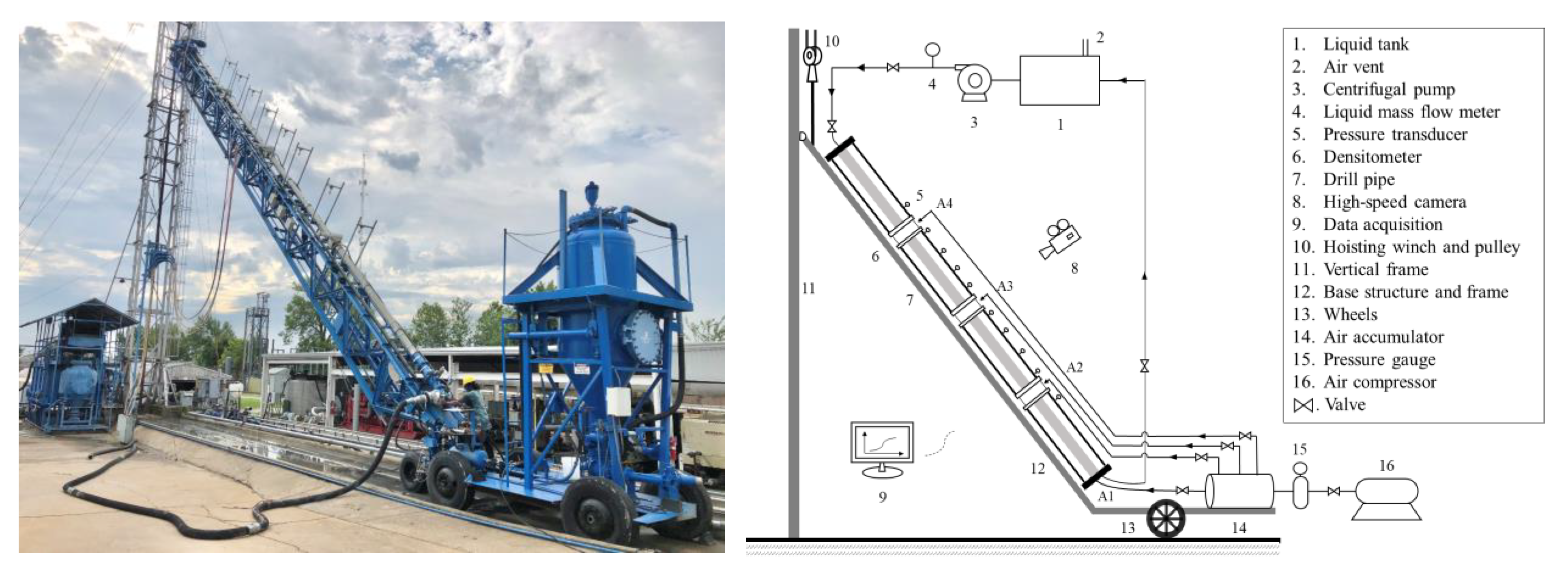
Experiments were conducted on the University of Tulsa Low Pressure–Ambient Temperature flow loop (LPAT). Figure 1 shows a general view and schematic view of the experimental facility.
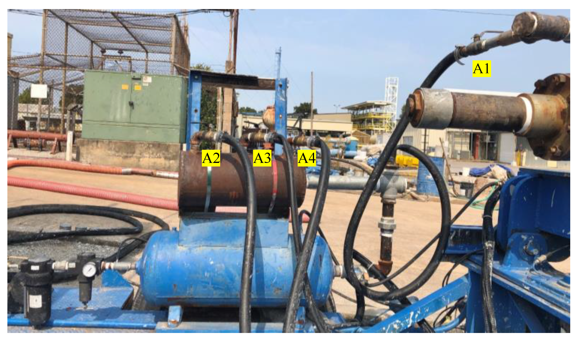
The test section was approximately 80 ft long and consisted of a 6 in. inner diameter (ID) transparent acrylic pipe. One end of the flow loop was attached to a vertically movable platform, while the other was connected to a trolley, which enabled the experimental operator to obtain any desired inclination angle between 4° to 90° from vertical [34,35,36,37]. Air as the gas phase was provided from an in-house air compressor (working capacity 0–125 psi, maximum 825 scfm capacity) to a buffer accumulator, through a regulator valve, which filled the buffer accumulator with air at a fixed pressure. There were four air valves corresponding to four injection ports at different locations (Figure 2). Port A1 was at the bottom of the flow loop, which was used to release the air in stagnant liquid, we called static condition. Ports A2 and A4 were installed approximately 20 ft from each end of the acrylic pipe, and Port A3 was located in the middle of the other two, as shown in the schematic view of the facility (Figure 1). Those three ports were used to inject air while the fluid was flowing downward, which was the so-called countercurrent flow condition. If necessary, air trapped at the top of the test section could be discharged directly to the atmosphere through a vent hose.
A 75 hp centrifugal mud pump (maximum capacity of 650 gpm) was used to supply water and low-rheology fluids, which were injected from the top of the flow loop. Figure 3a,b present the pump connection (inlet) and mud return (outlet), respectively. Fluids were pumped into the riser pipe (Figure 3a) to the top of the text section to create downward flow. At the bottom of the test section, a gate valve (Figure 3b) was used to control pressure in the system. Maintaining adequately high pressures was necessary to prevent the formation of vacuum bubble in the test apparatus—especially at inclinations near vertical.
For higher-rheology fluids, a triplex pump supplied by an oil-field service company was used. Liquid flow rate was measured using a Micro-MotionTM Emerson (St. Louis, MO, USA) mass flow meter. Figure 4 shows the flow rig built for this study.
The applied instruments include:
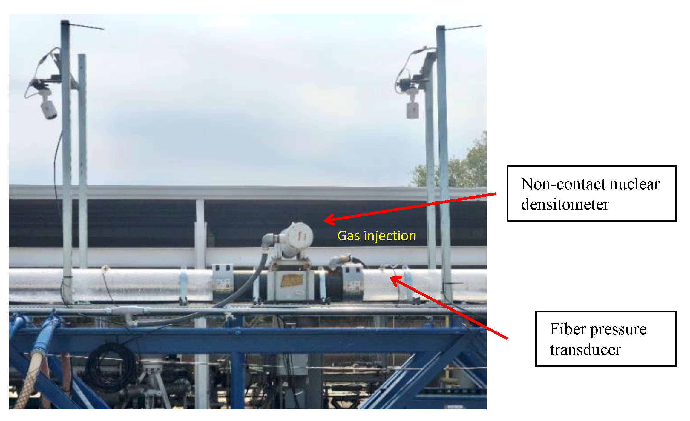
- Ten fiber optic pressure transducers, sensitive enough to detect small pressure variations with an accuracy of ±0.1%, were installed approximately 5 ft apart for differential pressure and velocity measurements. The pressure and time resolutions of the sensors were 0.001 psi and 0.1 sec, respectively.
- Three non-contact nuclear densitometers (X96S: Valencia, CA, USA) using a gamma radiation technique, which covered the entire pipe cross section area, for holdup and velocity measurements, were located approximately 20 ft from each end of the test section, and in its middle (spaced about 21 ft apart). The resolutions in density and time were 0.001 ppg and 0.1 sec, respectively. All densitometers were pre-calibrated by the full liquid/gas phase based on two-phase flow systems.
- Eight high-speed Amcrest security video cameras (Houston, TX, USA) were used for visualization. The non-Newtonian fluid applied in the experiment was opaque; therefore, cameras were only used in the water test.
Figure 5 shows a part of the instruments positioned along the test section.
Data acquisition was performed with LabViewTM (Austin, TX, USA) software which automatically recorded data, including mud flow rate, mixture density, inclination angle, pressure and differential pressure along the test section, and pressure and temperature at the inlet and outlet of the test section.
3.2. Experimental Procedure and Test Matrix
In this test, bentonite–water mixtures were used as the liquid phase. The bentonite–water mixtures were firstly prepared in a 100-barrel mud tank, then circulated into the system for at least 30 min to fully mix, waiting for at least 24 h for its full hydration. Rheology properties were checked before every new daily test.
In the static test, the fluid was firstly circulated at a high flow rate to make sure that the flow condition was homogeneous and to flush out the air in the test section. Then, the gate valve at the bottom was gradually closed while maintaining sufficient pressure on the system with the pump to prevent the formation of vacuum bubbles. At this point, the whole system was shut-in to avoid any effect of gas expansion on the bubble migration. Using the injection port A1, a finite burst of air was released. The pressure of the air accumulation chamber (Figure 2) was set anywhere between 20 to 50 psi above the pressure at port A1. Air was released for a 3 sec interval. When the bubble reached the top of the loop, the test was complete and data recording was stopped. The bubble was then purged from the system in preparation for another test.
In the countercurrent flow test, for each inclination angle, fluids were downwardly flowing at a given velocity; the Taylor bubble was released at port A2 and its rise velocity was measured. The bubble was then purged from the system in preparation for another test at a different countercurrent rate.
Water and four concentrations of bentonite–water mixtures were applied in the tests. The physical properties and test matrix are described in Table 1. All the experiments were carried out in inclined pipes at 4°, 15°, 30°, and 45° from vertical. In the present study, the gas–liquid interface tension of various concentrations of bentonite in water was applied from the experimental results of Dadashev et al. [38]—the range of the Eötvös number was 3212 < < 3405; therefore, the effect of on the movement of the Taylor bubble was not discussed in this work [15].
In Table 1, “10 lb/bbl BW” means 10 pounds per barrel bentonite–water mixture; “S” and “C” represent the tests conducted in static or countercurrent flow conditions, respectively; and and are the plastic viscosity and yield point in the Bingham plastic model, respectively. Rheological behavior is presented in Appendix B. As can be seen, countercurrent flow tests carried out in water were in a turbulent regime (Re > 2100) and a laminar flow regime (Re < 2100) in non-Newtonian fluids.
3.3. Determination of Bubble Velocity and Length
The main objective of this study was to investigate the migration of a single Taylor bubble in stagnant and downward non-Newtonian fluid flow in inclined pipes. The main hydrodynamic behaviors including translational velocity (), drift velocity (), and the length of the Taylor bubble () in the countercurrent flow condition were determined.
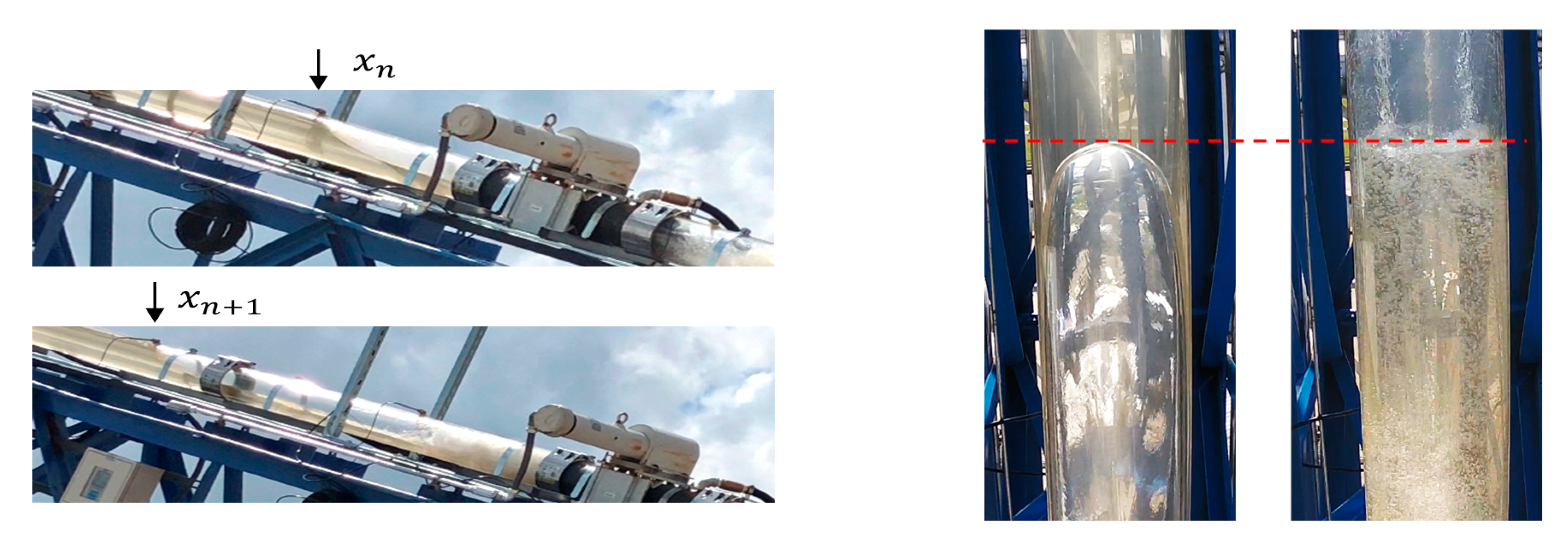
Velocities of Taylor bubbles are determined by the time for the Taylor bubble to travel between a fixed distance. Then, with the known of velocity, the length of Taylor bubble can be obtained by the time required for the bubble to pass through its own length (Figure 6).
In the present study, differential pressure (∆P) was applied to determine the velocity and length of Taylor bubbles.
3.3.1. Velocity of Taylor Bubbles
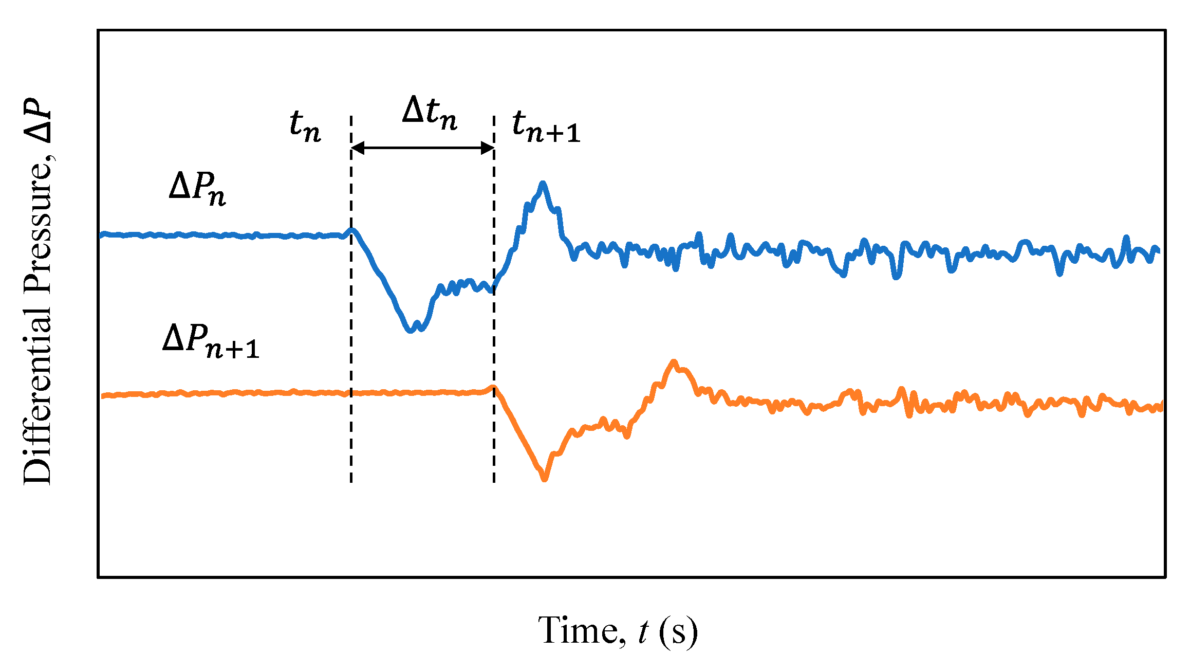
Figure 7 shows the differential pressure measured between two pressure transducers. ∆Pn measures the pressure difference between pressure transducer ∆Pn and ∆Pn+1, while ∆Pn+1 measures the pressure difference between ∆Pn+1 and ∆Pn+2. Considering a Taylor bubble moving inside the pipe, when its nose passes the pressure transducer PTn, the hydrostatic pressure at PTn decreases, the differential pressure ∆Pn starts decreasing synchronously. ∆Pn+1 remains stable until the bubble moves passed pressure transducer ∆Pn+1. Then, the same trend happens on ∆Pn+1.
Thus, the time between two sudden drops on the differential pressure curves is the duration of the Taylor bubble traveling between a fixed distance. The velocity of the Taylor bubble is obtained by averaging the velocities measured across the various possible pairings of pressure transducers:
3.3.2. Length of Taylor Bubbles
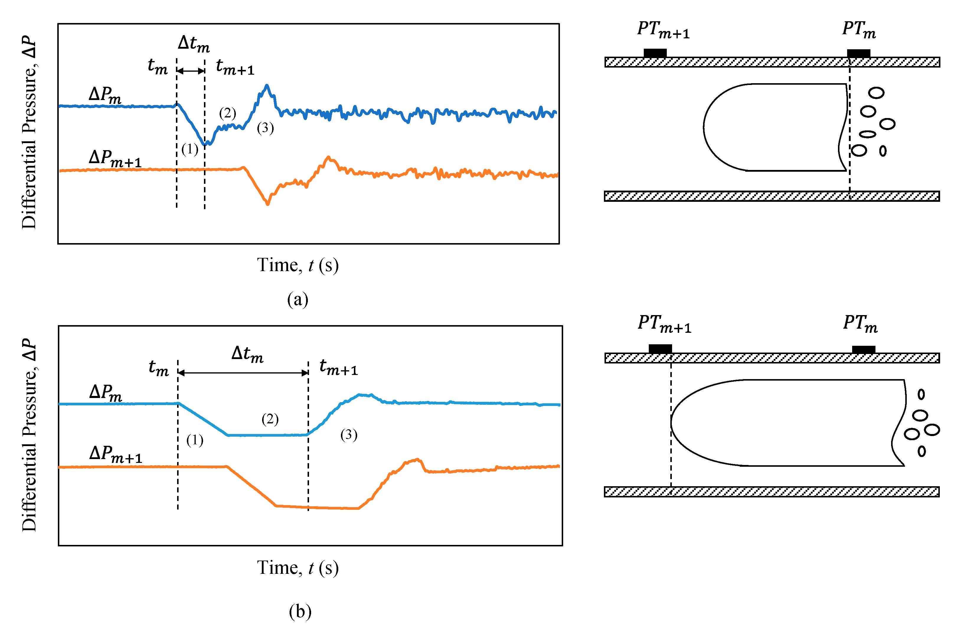
To determine the length of a bubble, two different scenarios are discussed.
The first scenario is when the length of Taylor bubble is shorter than the distance between two pressure transducers, as can be seen in Figure 8a. As the bubble reaches PTm, differential pressure ∆Pm starts decreasing reaching a minimum when the bubble tail reaches PTm. As the tail of the bubble moves past PTm, there is a slight increase in ∆Pm (shown between regions (1) and (2)). This is an artifact of the higher-pressure region behind the bubble being sensed by PTm. The fluid moving past the bubble creates a pressure reduction that is recovered in the wake of the upwardly migrating bubble. Region (2) is the period where the entire bubble length resides between PTm and PTm+1. The transition between regions (2) and (3) indicates when the bubble’s nose reaches PTm+1.
Then, a second scenario is considered where a bubble’s length is larger than the distance between two pressure transducers (Figure 8b). We start with the bubble reaching PTm. Region (1) signifies when the bubble’s nose is moving between PTm and PTm+1. Region (2) signifies when the bubble spans both PTm and PTm+1. Additionally, the transition between regions (2) and (3) signifies when the tail of the bubble passes PTm.
In each scenario, Δtm defines the time required for a Taylor bubble to pass PTm.
Thus, with the known bubble velocity and transit time across the sensor, the average length of Taylor bubble can be obtained:
4. Results and Discussion
The experimental data collected from both static tests and countercurrent flow tests were processed to obtain the velocity and length of the Taylor bubble.
4.1. Static Tests
4.1.1. Influence of and on
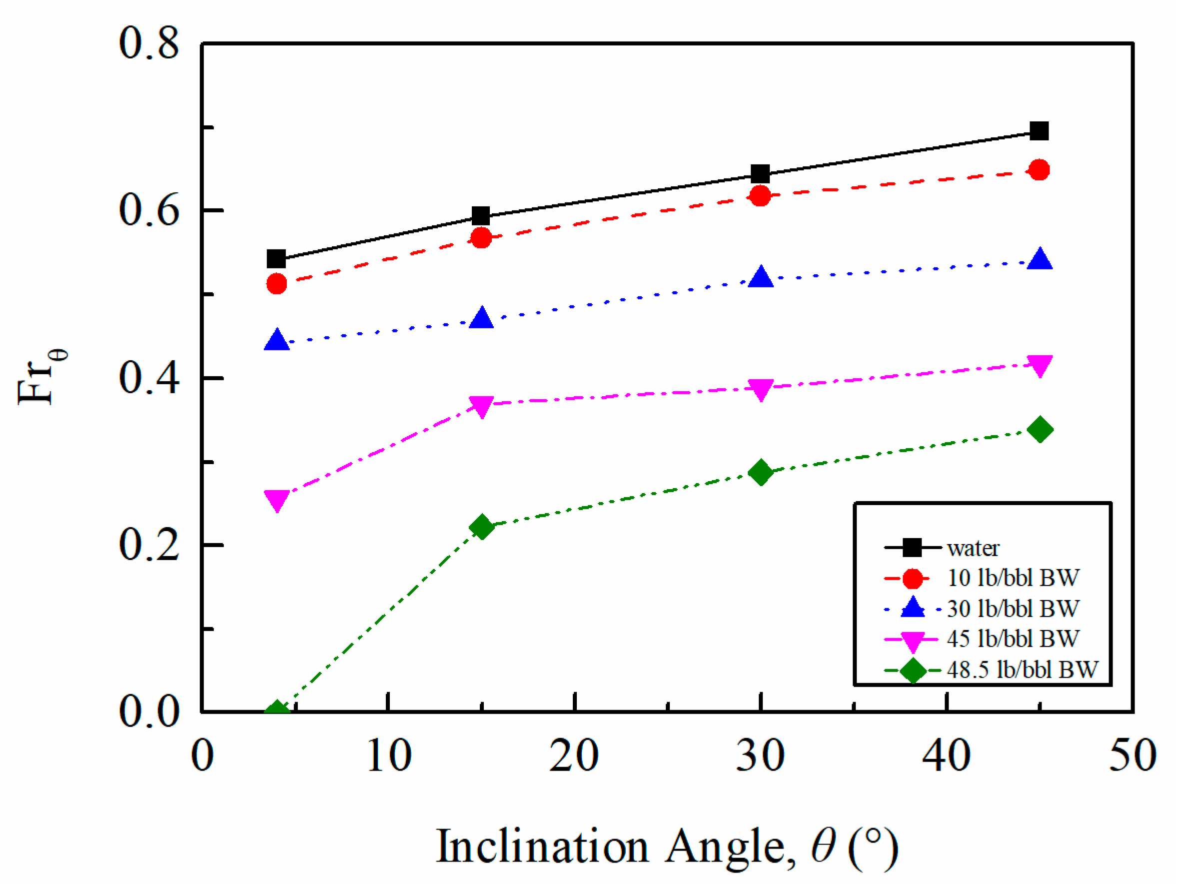
The propagation of a Taylor bubble through various stagnant liquids is presented in Figure 9, where the drift velocity is plotted as a function of inclination angles. Each line corresponds to a particular fluid. As can be seen, the dependence of drift velocity on inclination angle for non-Newtonian fluids is observed to be similar to Newtonian fluids. In each case, the drift velocity increases as the inclination angle increases. This result is consistent with Zukoski [40], who verified that the drift velocity would reach the maximum between 40° and 60°, and then decrease as the inclination approaches horizontal. Additionally, increasing the concentration of bentonite in our fluid, which increases plastic viscosity and the yield point, decreased drift velocity. This reduction was more significant at a lower inclination angle. It is noteworthy that an unexpected case was detected in 48.5 lb/bbl BW at 4°, where the Taylor bubble stopped moving soon after it entered the pipe. We will discuss this behavior in more detail in the subsequent section.
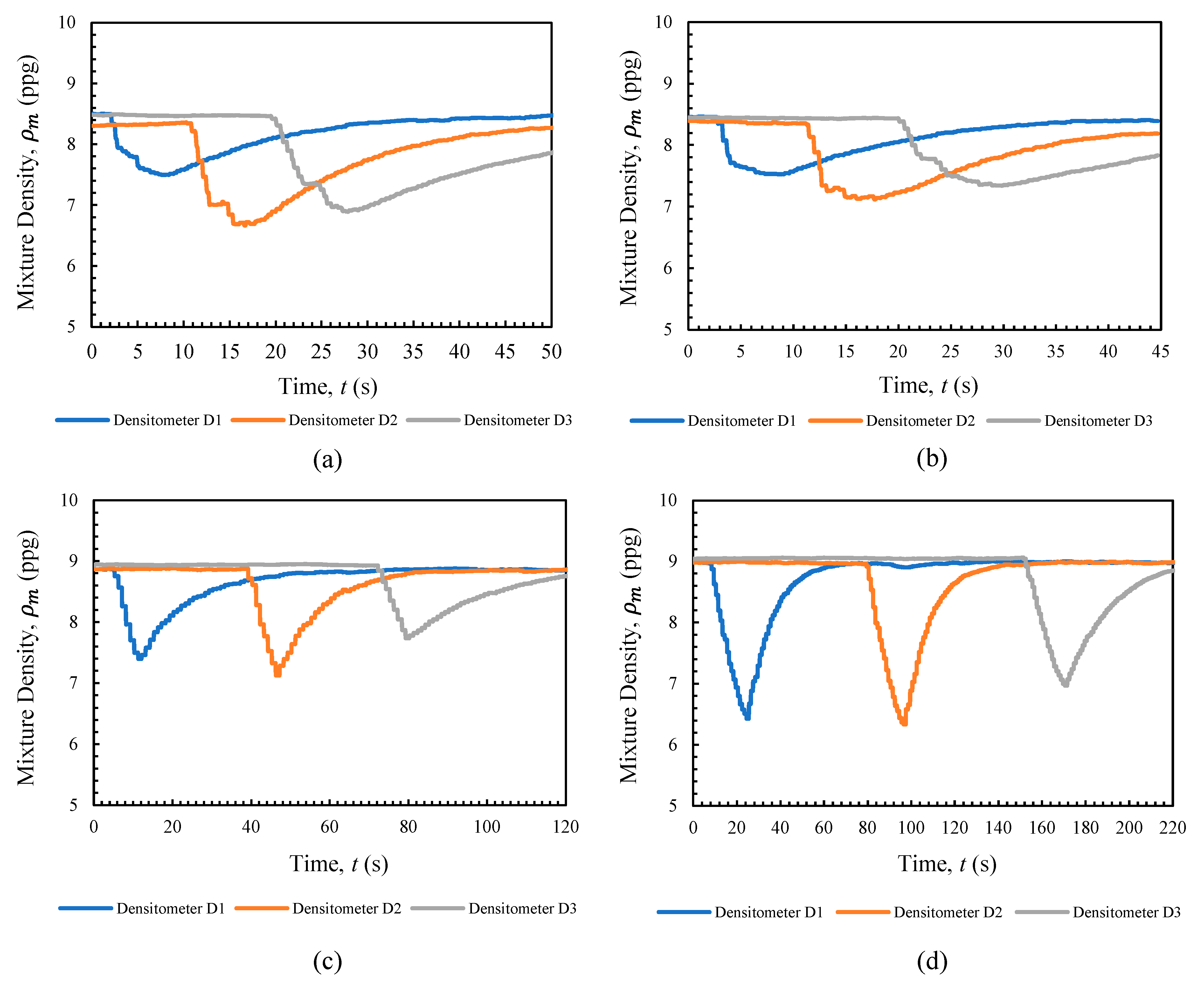
The lower drift velocities in a more viscous fluid can be explained by the higher drag forces imposed on the bubble’s flanks and by changes in the shape of the bubble’s nose. Figure 10a–d illustrate the air–liquid mixture density (ρm) change with time as the bubble migrates past the densitometers at 45° from vertical. As the Taylor bubble nose reached the densitometer, the mixture density dropped because of the lower density of air. It also shows that there was a flow development between densitometers D1 and D2 after the gas bubble was released. The mixture density can be obtained by the relationship:
where is the void fraction defined as the fraction of the cross-sectional area of the channel that is occupied by the gas phase. In fluids with lower concentrations of bentonite (Figure 10a,b), the mixture density gradually decreased during the passage of the bubble’s nose. However, for higher concentrations of bentonite (Figure 10c,d), a steeper decrease in the mixture density occurred, indicating a steeper increase in . This indicates that the curvature of the Taylor bubble’s nose is blunted with a significant increase in viscosity and yield point. This is also suggested by the experimental work conducted by Carew et al. [24], who reported that an increase in the liquid viscosity caused the nose region of the bubbles to become blunter and led to a decrease in the bubble rise velocities.
In this study, we used apparent viscosity as a singular measure of a non-Newtonian fluid’s rheological state, which was useful in the formulation of our generalized bubble drift correlation. The bentonite–water mixtures used in this study exhibited non-Newtonian rheological behavior having a yield point, which can be represented by the Herschel–Bulkley model:
where is the shear stress, is the yield point, is the consistency index, is the shear rate, and is the flow index. For a single Taylor bubble rising in stagnant liquid, the characteristic shear rate around the bubble can be scaled as [18]:
Thus, the apparent viscosity is given by:
In this study, bentonite–water mixtures were represented by a Bingham plastic model, having a yield point. Thus, the in Equation (36) was the plastic viscosity (, and became unity.
Therefore, the apparent viscosity for a Bingham plastic fluid can be written as:
From Equation (39), we know that when the pipe diameter is fixed, is then governed by both fluid properties and drift velocity.
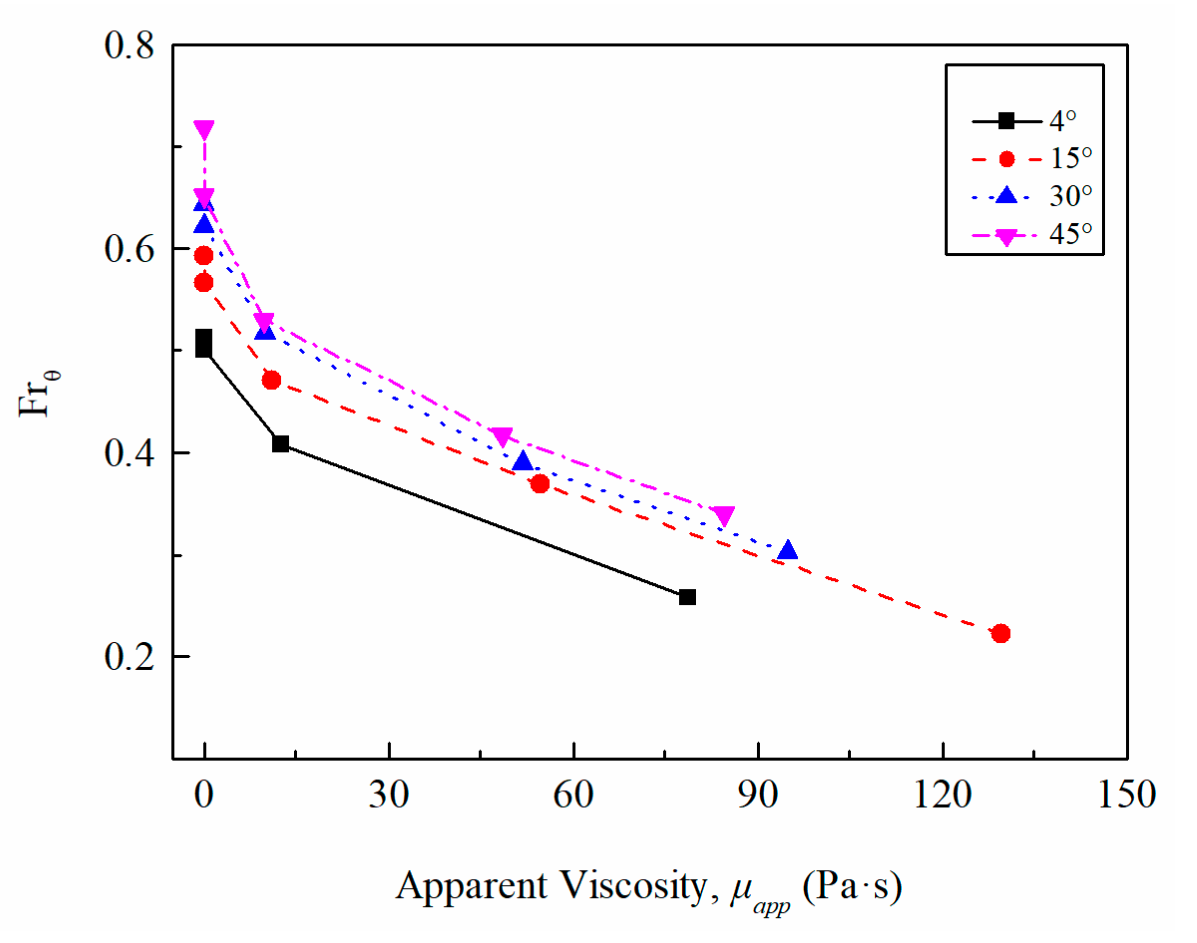
Based on Equation (39), the quantitative influence of apparent viscosity on drift velocity can be obtained—which is illustrated in Figure 11. For all fluids studied, the drift velocity decreased dramatically with the increase in apparent viscosity, and this reduction became even more significant when the inclination angle decreased. The apparent viscosity for Bingham plastic fluids in terms of plastic viscosity and yield point became significant when the plastic viscosity and yield point increased with the concentration of bentonite, making it harder for the liquid film to flow around the bubble.
4.1.2. Proposed Drift Velocity Correlation
Based on the variation of drift velocity with the inclination angles and apparent viscosity ranging from 0.001 < < 129 , the proposed correlation (3212 < < 3405) combines Bendiksen et al. [17] in terms of and a yield–power-law correlation in terms of [41,42]. The mathematical form of the proposed drift velocity correlation is given as:
This proposed correlation is similar to Bendiksen et al. [17], and the proportional value of the horizontal drift velocity component is modified as 0.45, which was inspired by Gokcol et al. [19] and suggested by Bhagwat and Ghajar [10]. Fitted values of these parameters are given as a = 0.99416, b = −0.18458, c = 0.21337, d = 0.48996, and e = 0.02661, respectively.
Performance of Proposed Correlation
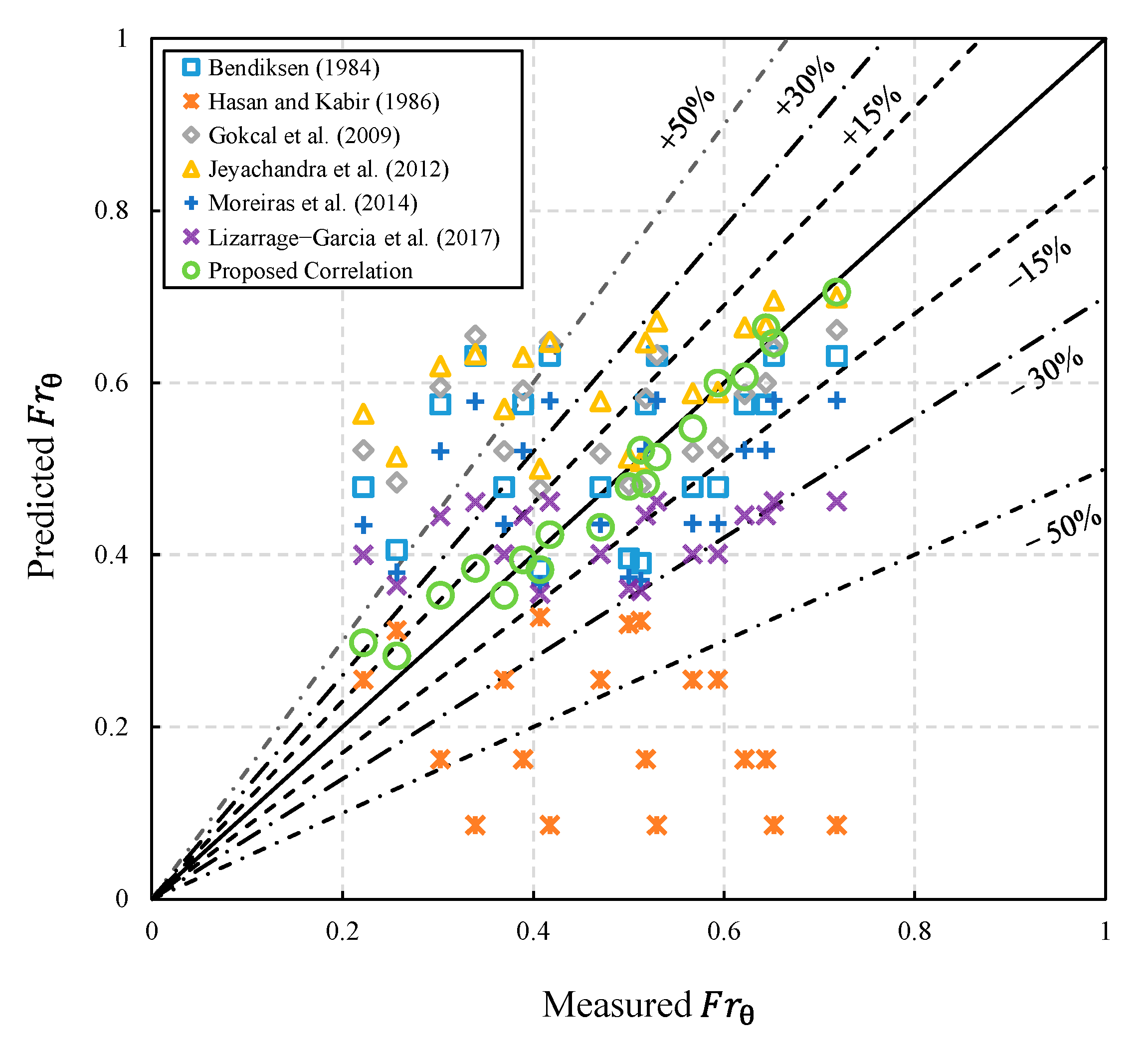
Figure 12 presents the performance of the proposed and comparative correlations against measured drift velocity (drift velocity measured in 48.5 lb/bbl at 4°, which is zero, is excluded). The correlations developed by Carew et al. [24] and Majumdar and Das. [25] for power-law fluids were not applied for performance-comparison. Those correlations utilize n and k and are, therefore, not aligned with our Bingham plastic model. The dashed lines are the ±15%, ±20%, and 50% error bands showing in Figure 12. It is obvious that the proposed correlation shows good performance, slightly under-predicting the drift velocity. The major differences among correlations occurred in the relatively low value of corresponding to non-Newtonian fluids. The Gokcal et al. [19], Moreiras et al. [22] and Jeyachandra et al. [21] correlations show better prediction when was high and tend to overestimate the drift velocity when < 0.4, which is thought to be caused by over-predicting the influence of viscosity on drift velocity. Bendiksen [17] and Hasan and Kabir [13] correlations were developed by water, which could have a relatively better performance for low-viscosity fluids.
Table 2 summarizes the quantitative performance of different correlations by using the following statistical parameters:
Mean difference, :
Mean absolute relative difference, :
Standard deviation, :
As shown in Table 2, the proposed correlation predicted 90% of data points within ±15% error bands and 85% within ±10%. The proposed correlation had a mean absolute relative difference value of 0.0702. The Gokcal et al. [19] correlation gave the best performance among the comparative correlations within ±15%, but fewer data points were within the ±15% error band compared with the Jeyachandra et al. [21] correlation. The poor performance of the Hasan and Kabir [18] correlation is thought to be because of the low-viscosity fluid which they used to develop the correlation. Based on the performance of different correlations for predicting drift velocity, we know that although the behaviors of drift velocity against inclination angles between Newtonian and non-Newtonian fluids are similar, those correlations developed for Newtonian fluids may not be applicable for non-Newtonian fluids.
Validation of the Proposed Correlation
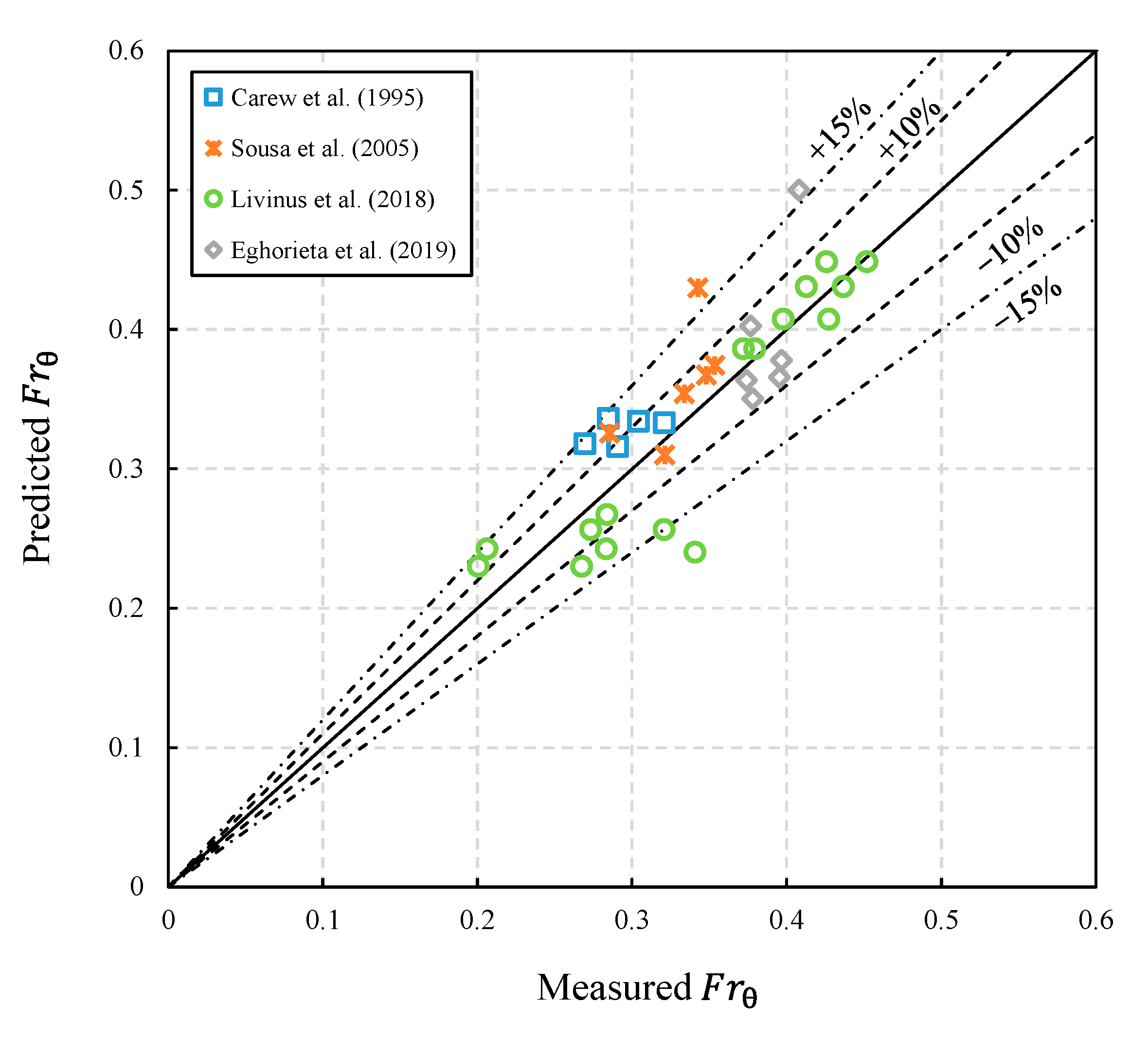
An additional database collected from Carew et al. [24], Sousa et al. [28], Eghorieta et al. [43], and Livinus et al. [44] was applied to validate the applicability of the proposed correlation. The database is summarized in Table 3 (inclination angles are measured from vertical). The non-Newtonian fluids (power-law) experimental data reported by Carew et al. [24] and Sousa et al. [28] are for different concentrations of CMC and Carbopol, covering a range of pipe diameters and liquid viscosities. The Newtonian fluids used by Eghorieta et al. [43], and Livinus et al. [44] were water and oil, respectively.
According to the rheological model for Newtonian and power-law fluids, the apparent viscosity for a Newtonian fluid is the same as liquid viscosity; the yield point in a power-law fluid is zero. Thus, Equation (38) can be written as:
The performance of the proposed correlation against the new database is shown in Figure 13. It is evident that the proposed correlation exhibits good experimental performance for both Newtonian and non-Newtonian fluid data points, but slightly over-predicted by Carew et al. [24], who obtained data from small diameter pipes. The proposed correlation shows a small value of mean absolute relative difference of 0.09614. This is attributed to the apparent viscosity used in this study, which can be applied for both Newtonian and non-Newtonian fluids.
4.2. Countercurrent Flow Tests
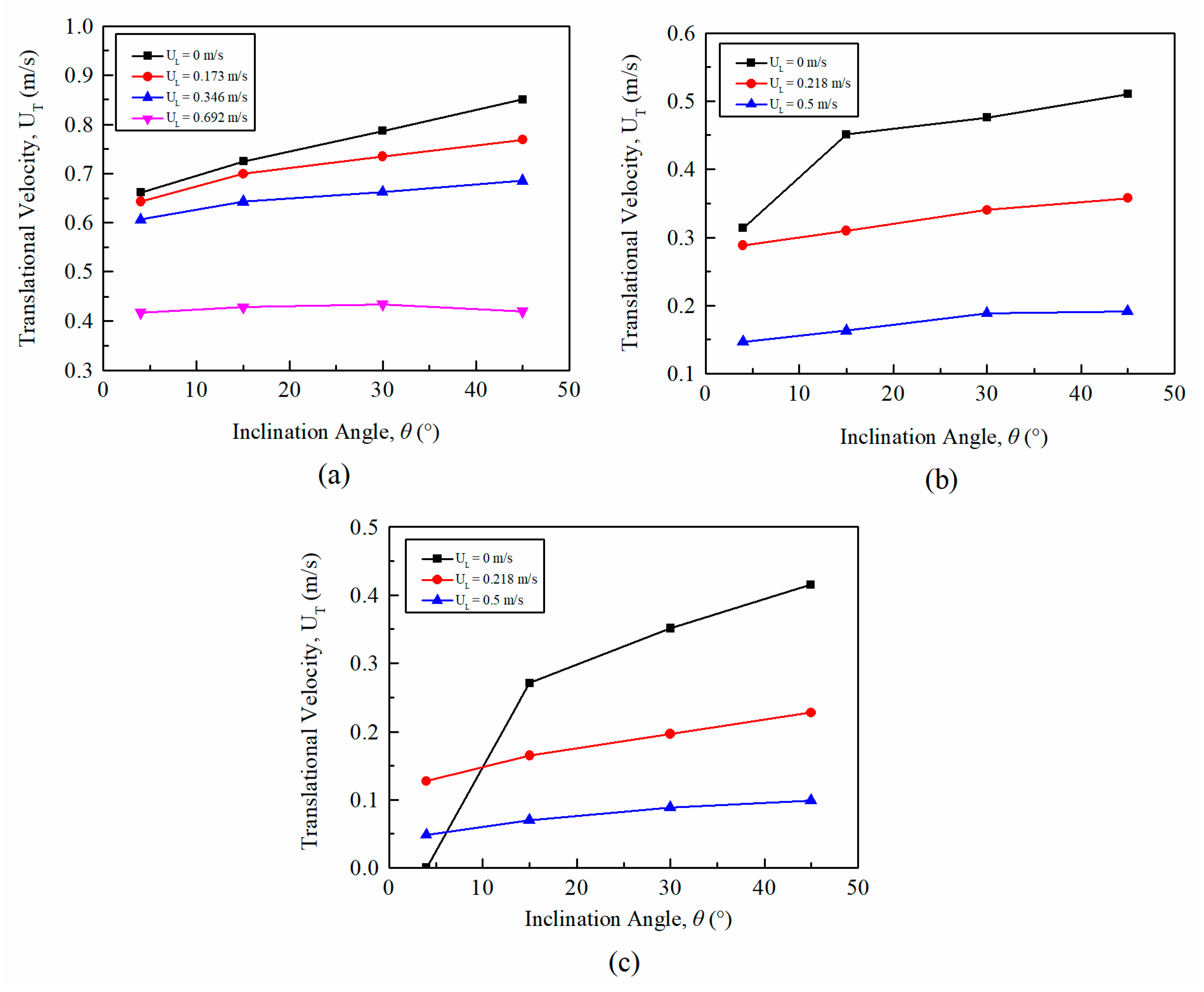
4.2.1. Influence of on
In Figure 14, the translational velocity is plotted against inclination angles (curves with = 0 m/s for reference). As can be seen, the translational velocity increases with the increase in inclination angle; this behavior is similar to the results obtained in static condition because of an increase in the drift velocity.
4.2.2. Influence of Liquid Viscosity on
Figure 15a,b indicate the influence of liquid viscosity induced by different concentrations of bentonite–water solutions on bubble velocity under fixed downward liquid velocities. As can be seen, in agreement with the observations in stagnant liquid test, an increase in the liquid viscosity results in a reduction in the bubble velocity for a given countercurrent flow liquid velocity. This reduction in the translational velocity is qualitatively the same as the inclination angle increases.
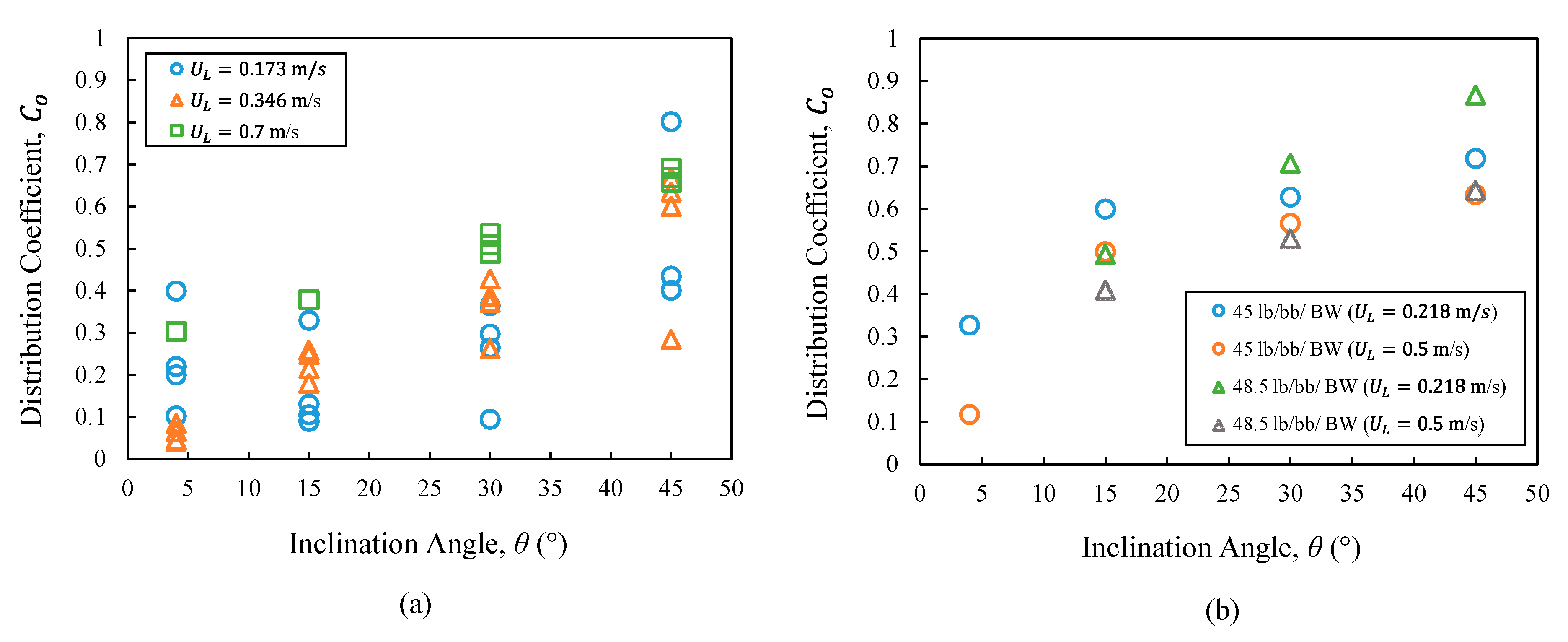
4.2.3. Distribution coefficient,
Once the measured in countercurrent flow and measured from static test are obtained, the distribution coefficient can be calculated by Equation (2) in the form of . Figure 16a,b plot against the inclination angles for both water and non-Newtonian fluids. tends to increase with the increase in inclination angle.
The general increasing trend of with wellbore inclination is the result of increasing more rapidly than as increases. is measured under static fluid conditions; in a near-vertical wellbore, a Taylor bubble’s shape is relatively concentric, thus minimizing (because it is hydrodynamically inefficient). As wellbore inclination departs from vertical, buoyancy forces lateral to the bubble increasingly deform its shape to make the bubble is more hydrodynamically efficient, resulting in significantly higher values. , on the other hand, is the translational velocity of a Taylor bubble that, because of countercurrent flow, is always in a non-concentric (and, thus, a hydrodynamically efficient) shape, regardless of the flow conduit’s inclination for all our experiments. Hence, a progressively increasing drives greater increases in measured under static conditions (see Figure 9) than measured under constant conditions (see Figure 14).
According to Zuber and Findley [45], the value of could be less than unity when the ratio of the volumetric gas concentration evaluated at the wall, , and at the centerline, , of the duct is greater than one, . This occurs when a Taylor bubble flows inside an inclined pipe, where a loss of symmetry is observed due to the component of buoyancy force leading to the liquid film thickness between the top wall of the pipe and Taylor bubble decreasing when inclination angle is increased from vertical. Although Zuber and Findley’s insight comes from an analysis based on a co-current flow perspective, their finding correctly applies to our countercurrent test results, regardless of inclination. This is because our imposed countercurrent flow conditions always result in a non-concentric Taylor bubble that tracks along the flow conduit wall.
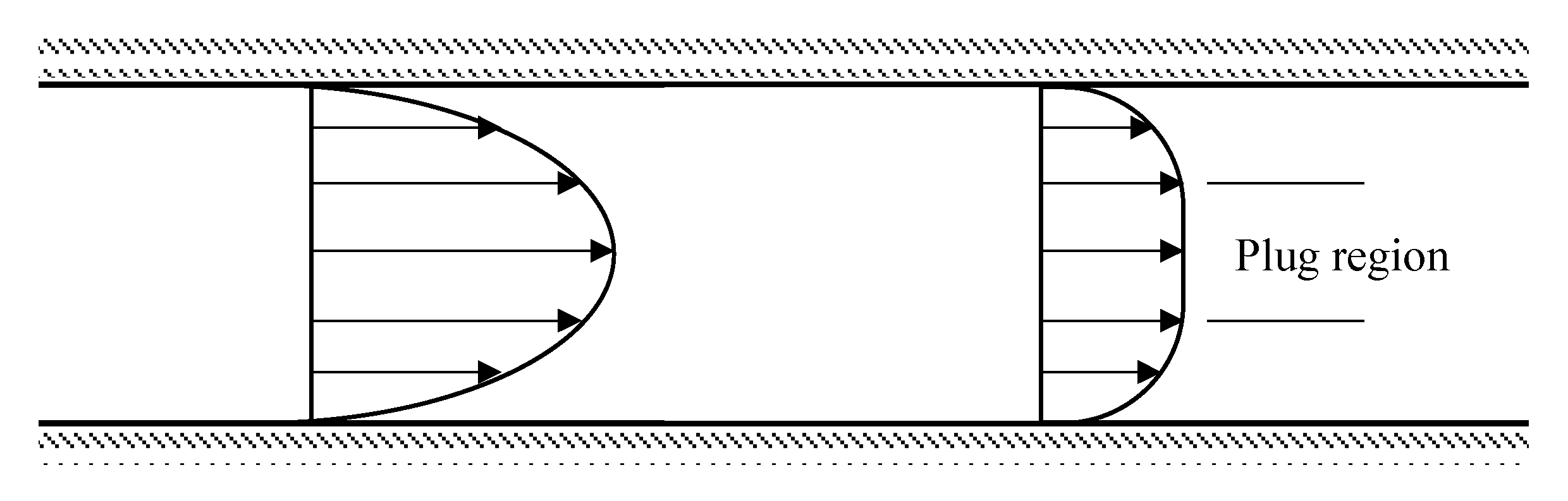
Additionally, under co-current flow conditions, values obtained for non-Newtonian fluid is generally greater than that in Newtonian fluid (e.g., water), which is due to the different flow profiles between Newtonian fluids and non-Newtonian fluids (Figure 17). For Newtonian fluid (Poiseuille flow), the flow profile is parabolic, while for shear-thinning non-Newtonian fluid, such as a Bingham plastic, the profile of the flow is flatter in the middle, called the plug region, and decays faster towards the wall. For a Taylor bubble rising in co-current flow liquid in a vertical orientation, the leading nose will follow the highest velocity, which is at the center of the pipe. In contrast, the bubble will tend to follow the lowest liquid velocity which is at the wall in countercurrent flow liquid. As shown in Figure 16, under countercurrent conditions, there is little difference in the values of between Newtonian and non-Newtonian fluids. Again, this is because our imposed countercurrent flow conditions always result in a non-concentric Taylor bubble that tracks along the conduit wall. A break from this trend only occurs at higher bentonite concentrations where viscous forces are so high that plug flow occurs (i.e., when = 1 and = 0 m/s).
4.2.4. Length of Taylor Bubbles
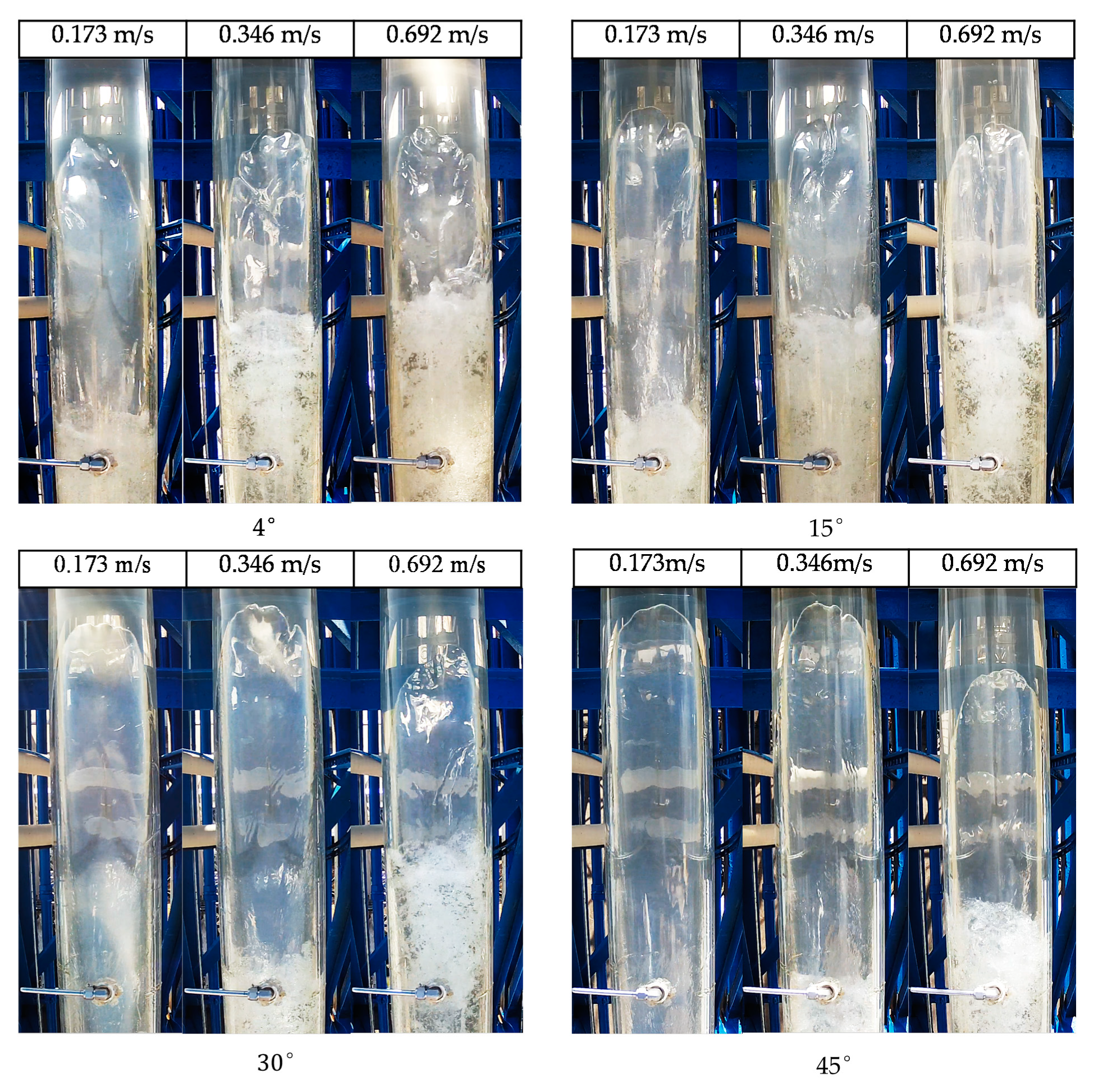
The influence of downward flowing velocity and inclination angle on the length of Taylor bubble (the volume of the Taylor bubble is the same in all cases) in water is visualized in Figure 18a–d. The reason why all pipes appear to be vertically orientated is because the camera was mounted right above the pipe. As shown in Figure 18, the bubble becomes asymmetric with a fluctuating nose under countercurrent flow condition. The liquid velocities of water from left to right for each figure are 0.173 m/s, 0.346 m/s, and 0.692 m/s, respectively. In higher downward flowing velocities, bubble surface waves start from the nose and are swept down to the tail. It is obvious that for each inclination angle, the length of the Taylor bubbles decrease with the increase in downward liquid flow velocity because of increasing liquid film thickness/holdup and increasing entrainment of gas into the wake region. However, no direct relationships between the Taylor bubble length and the inclination angle were observed.
Influence of and on
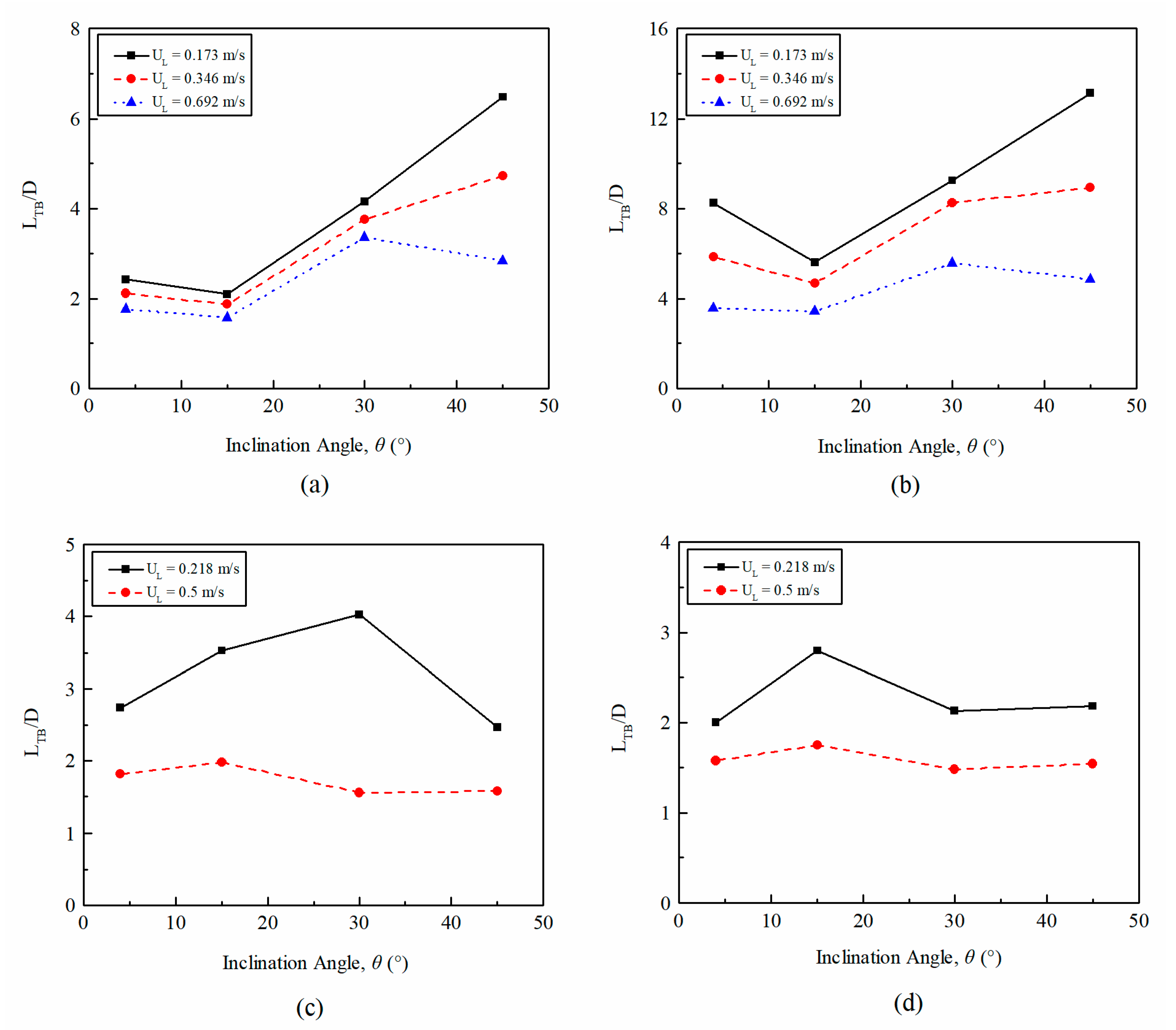
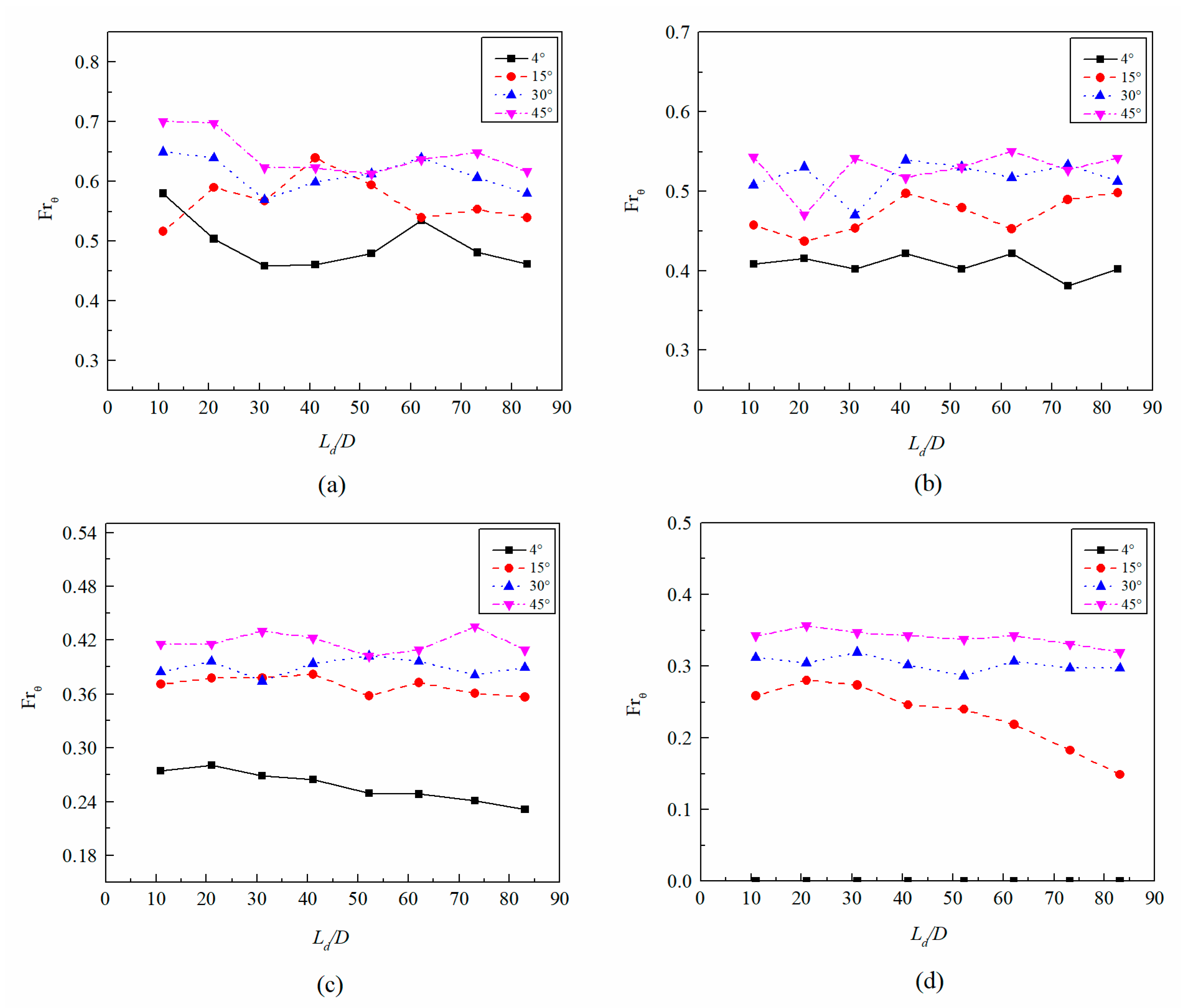
Figure 19a,b present the dimensionless bubble length ( as a function of inclination angle under different downward liquid flow velocities for the experiments performed with Newtonian and non-Newtonian fluids. Figure 19a,b show the length of two different volumes of the Taylor bubbles measured in water. Figure 19c,d illustrate the bubble length measured in 45 lb/bbl BW and 48.5 lb/bbl BW, respectively. As can be seen, two different volumes of Taylor bubbles present similar behavior with the change of inclination angles and liquid velocities. It is evident that the length of Taylor bubble decreases as the downward liquid velocity increases, independently of the fluids considered.
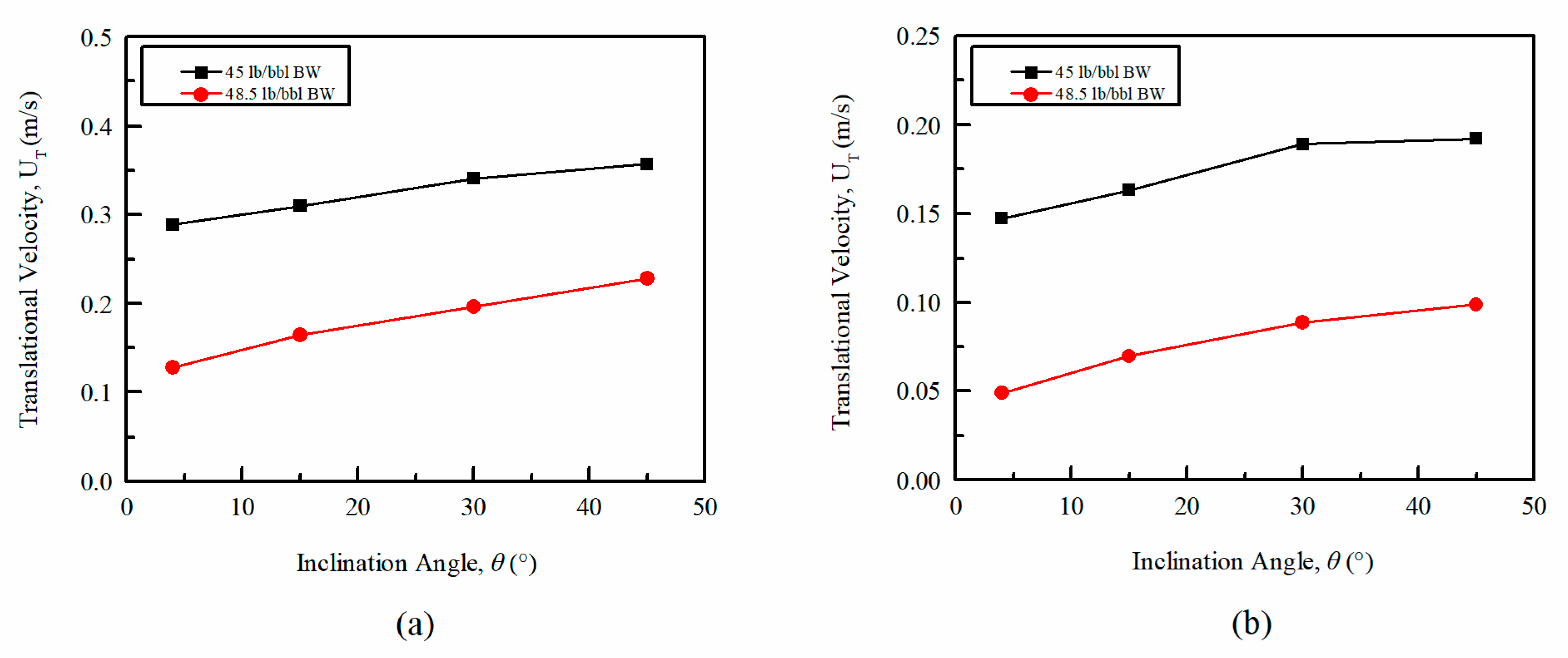
Influence of Liquid Viscosity on
The influence of liquid viscosity induced by higher concentration of bentonite on under fixed downward liquid velocities is presented in Figure 20a ( = 0.218 m/s) and Figure 20b ( = 0.5 m/s). As can be seen, an increase in the liquid viscosity results in a reduction in the bubble length for a given countercurrent flow velocity. As discussed before, the reduction in the translational velocity as the liquid viscosity increases is qualitatively the same as the inclination angle increases. However, the decrease in the bubble length due to viscosity increase is different as the inclination angle increases, which indicates that the translational velocity is independent of bubble length.
4.3. Unexpected Case: The Stagnant Taylor Bubble
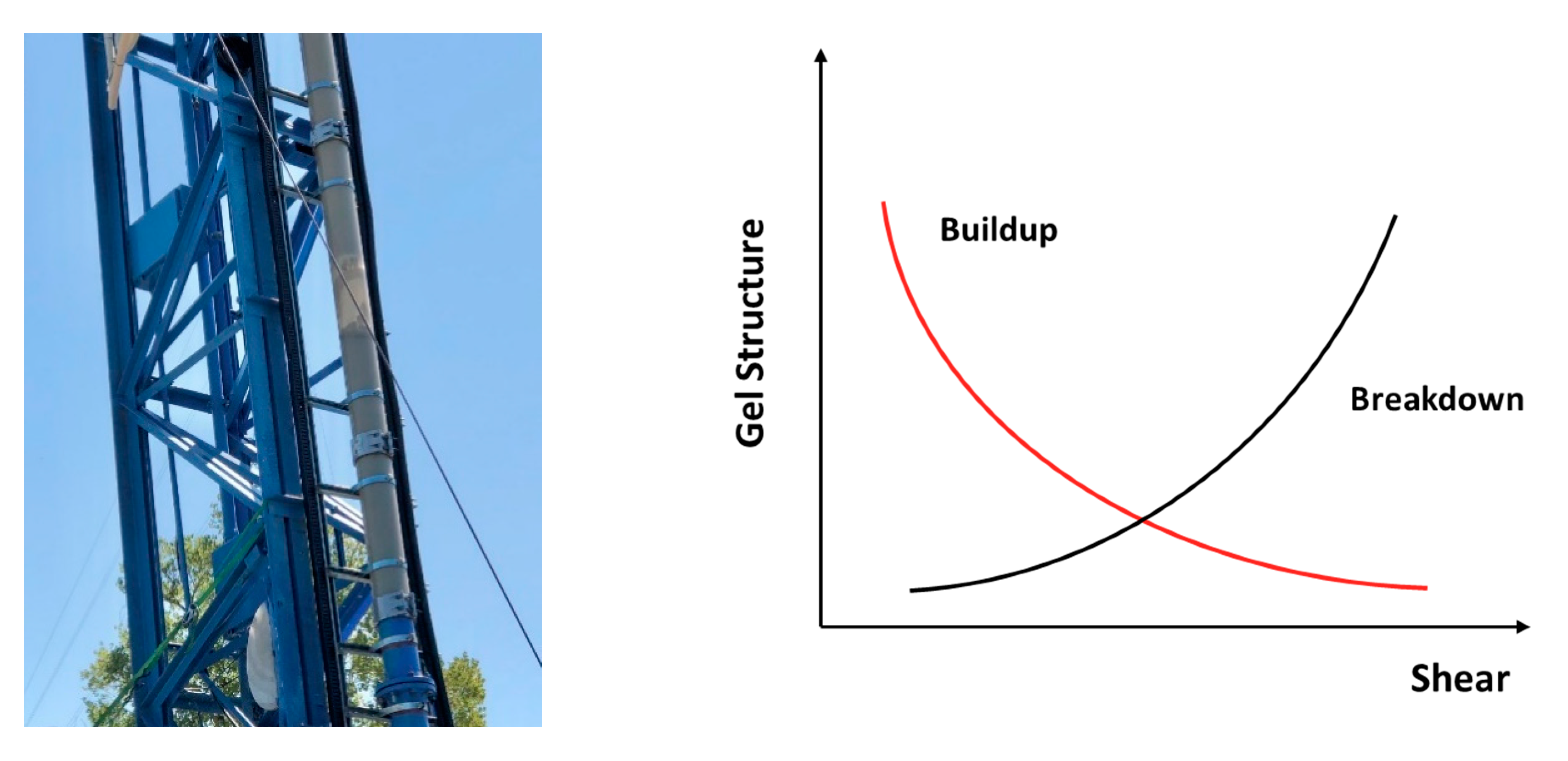
In the static test of 48.5lb/bbl BW at 4°, the Taylor bubble stopped moving soon after it entered the pipe (Figure 21). This was because of the thixotropic properties of bentonite–water mixtures. When a thixotropic material is sheared, the buildup and breakdown of gel structure processes compete, and a dynamic equilibrium eventually results. For high concentrations of bentonite, a strong gelled structure is formed over little time when not subject to shearing. This provides resistance to the bubble movement, eventually resulting in a stagnant bubble.
The effect of gel strength can be directly obtained by comparing the drift velocities at different positions along the pipe. Figure 22a–d show the drift velocity measured at different pressure transducers against the distance it travels, each line representing a particular inclination angle. As can be seen, in the lower concentrations, the drift velocity remains relatively constant during the bubble movement in all inclination angles, while a slight decrease in drift velocity can be observed in 45 lb/bbl bentonite at 4° as the bubble migrates (Figure 22c), then a great reduction in drift velocity is shown in 48.5 lb/bbl bentonite at even higher inclination angles (Figure 22d), which is owing to the lower drift velocity at low inclination angles corresponding to a longer stationary time, eventually resulting in a stronger gel structure.
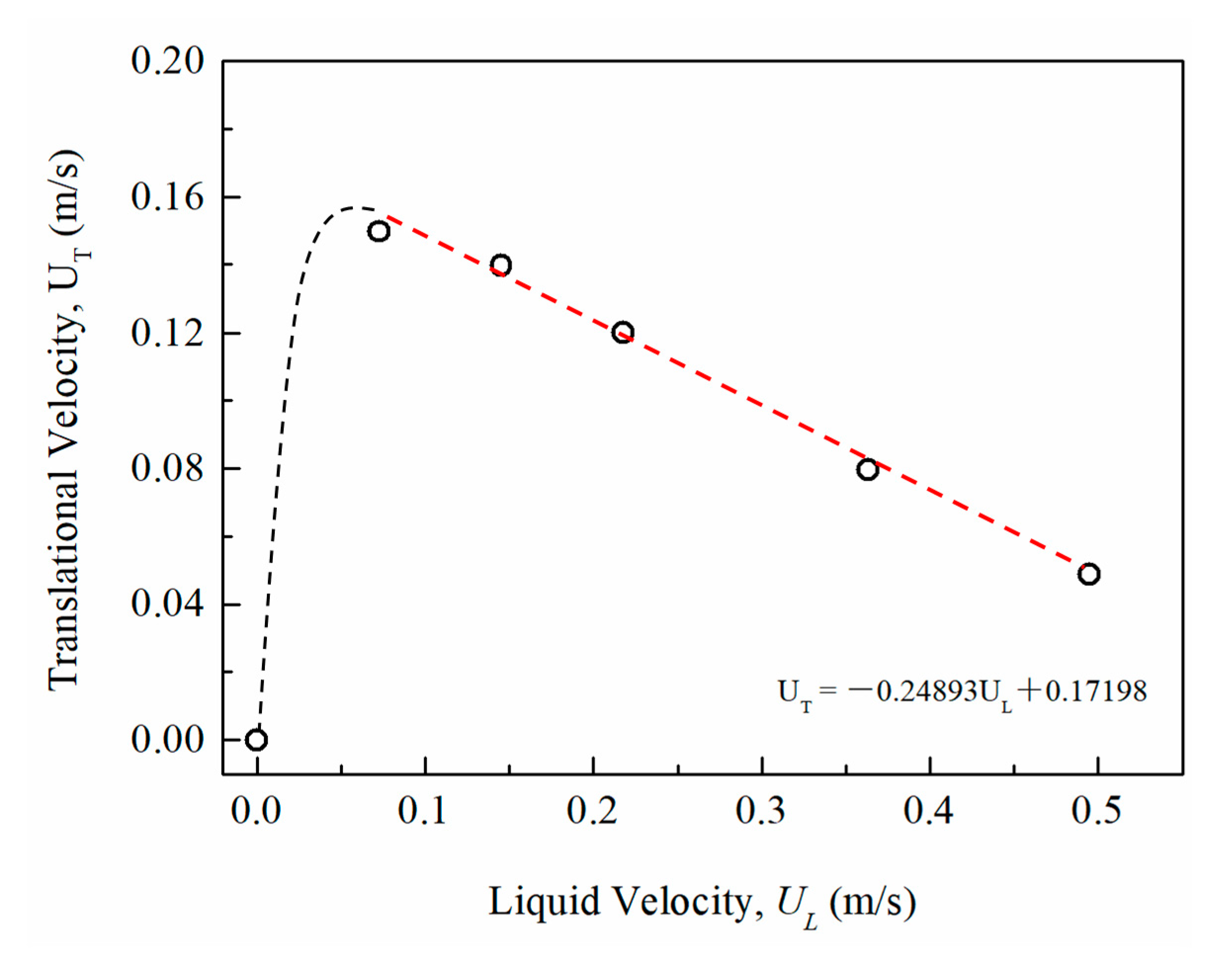
Gel structure breakdown can be induced by shearing. Figure 23 shows the propagation of a Taylor bubble against a range of downward liquid velocities (0.073 m/s 0.5 m/s) at 4° in 48.5 lb/bbl bentonite–water mixtures after it has been circulated. Notice that at = 0 m/s the bubble migration stops. This is due to the fluid gelling tendency. However, under a shearing condition ( > 0 m/s) the gel structure is broken, and the bubble migration becomes dependent on . The relationship between the and under countercurrent flow condition can be fitted in a linear function (red dash line), as suggested in Equation (2). The second constant (0.172 m/s) is normally interpreted as the drift velocity. In this case, however, the strong gelling nature of the fluid invalidates this interpretation.
5. Conclusions
The movement of single Taylor bubble rising in stagnant and downward flowing non-Newtonian fluids in inclined pipes has been experimentally studied. The following conclusions can be drawn:
- 1.
- A flow rig has been built for the purpose of investigating the movement of a single Taylor bubble rising in stagnant and downward flowing bentonite–water mixture in inclined pipes (4° < < 45° from vertical).
- 2.
- The measured drift velocity () data presented in this study can contribute to improve the knowledge of a single Taylor bubble rising in stagnant non-Newtonian fluids having a yield point.
- 3.
- The experimental results indicate that for all fluids tested, the bubble velocity increased as the inclination angles () were increased, while velocity decreased with an increase in plastic viscosity () and yield point (). The length of the Taylor bubble () decreased as the downward flowing liquid velocity () and were increased. The bubble velocity was found to be independent of the .
- 4.
- A reduction in drift velocity along its migration was detected, because increasing the concentration of bentonite results in a strong gel strength buildup. Eventually, a stagnant Taylor bubble can occur.
- 5.
- The drift velocity is formulated by combining a function of and a yield–power-law correlation in terms of apparent viscosity (), making it applicable for non-Newtonian fluids with the Eötvös number () ranging from 3212 to 3405 and apparent viscosity () ranging from 0.001 to 129 . The proposed correlation shows good performance for predicting drift velocity from both the present study (mean absolute relative difference is 0.0702) and a new database (mean absolute relative difference is 0.09614).
Author Contributions
Y.L. performed the experiments, analyzed the data, and wrote the paper; E.R.U. conceived, designed, and performed the experiments, and edited the manuscript; E.M.O. designed the experiments, led the project, and advised on the whole process of the manuscript preparation. Each author has contributed to the present paper. All authors have read and agreed to the published version of the manuscript.
Funding
This research was supported by the Chevron Corporation.
Institutional Review Board Statement
Not applicable
Informed Consent Statement
Informed consent was obtained from all subjects involved in the study.
Data Availability Statement
The data presented in this study are available in Appendix A.
Conflicts of Interest
The authors declare no conflict of interest.
Appendix A
Table A1 summarizes the experimental data for single Taylor bubbles rising in stagnant water and Bingham plastic fluids in inclined pipe, to provide traceability from the experimental measurements to the final conclusions.

Table A1.
Experimental Taylor bubble drift velocity data in inclined pipes.
| Fluid | (°) | ID (m) | |||||||
|---|---|---|---|---|---|---|---|---|---|
| Water | 4 | 0.152 | 998 | 0.001 | 0 | 0.001 | 3240 | 0.661 | 0.541 |
| 15 | 0.152 | 998 | 0.001 | 0 | 0.001 | 3240 | 0.725 | 0.593 | |
| 30 | 0.152 | 998 | 0.001 | 0 | 0.001 | 3240 | 0.787 | 0.644 | |
| 45 | 0.152 | 998 | 0.001 | 0 | 0.001 | 3240 | 0.850 | 0.695 | |
| 10 lb/bbl BW | 4 | 0.152 | 1015 | 0.002 | 0.75 | 0.189 | 3212 | 0.627 | 0.513 |
| 15 | 0.152 | 1015 | 0.002 | 0.75 | 0.167 | 3212 | 0.693 | 0.567 | |
| 30 | 0.152 | 1015 | 0.002 | 0.75 | 0.153 | 3212 | 0.756 | 0.618 | |
| 45 | 0.152 | 1015 | 0.002 | 0.75 | 0.146 | 3212 | 0.792 | 0.648 | |
| 30 lb/bbl BW | 4 | 0.152 | 1047 | 0.027 | 41.6 | 12.765 | 3314 | 0.540 | 0.442 |
| 15 | 0.152 | 1047 | 0.027 | 41.6 | 11.045 | 3314 | 0.573 | 0.469 | |
| 30 | 0.152 | 1047 | 0.027 | 41.6 | 10.042 | 3314 | 0.633 | 0.518 | |
| 45 | 0.152 | 1047 | 0.027 | 41.6 | 9.816 | 3314 | 0.660 | 0.540 | |
| 45 lb/bbl BW | 6 | 0.152 | 1063 | 0.076 | 162 | 78.666 | 3364 | 0.314 | 0.257 |
| 15 | 0.152 | 1063 | 0.076 | 162 | 54.734 | 3364 | 0.451 | 0.369 | |
| 30 | 0.152 | 1063 | 0.076 | 162 | 51.963 | 3364 | 0.476 | 0.389 | |
| 45 | 0.152 | 1063 | 0.076 | 162 | 48.471 | 3364 | 0.510 | 0.417 | |
| 48.5 lb/bbl BW | 4 | 0.152 | 1076 | 0.101 | 230 | undefined | 3405 | 0 | 0 |
| 15 | 0.152 | 1076 | 0.101 | 230 | 129.443 | 3405 | 0.271 | 0.222 | |
| 30 | 0.152 | 1076 | 0.101 | 230 | 94.803 | 3405 | 0.351 | 0.287 | |
| 45 | 0.152 | 1076 | 0.101 | 230 | 84.606 | 3405 | 0.415 | 0.339 |
Appendix B
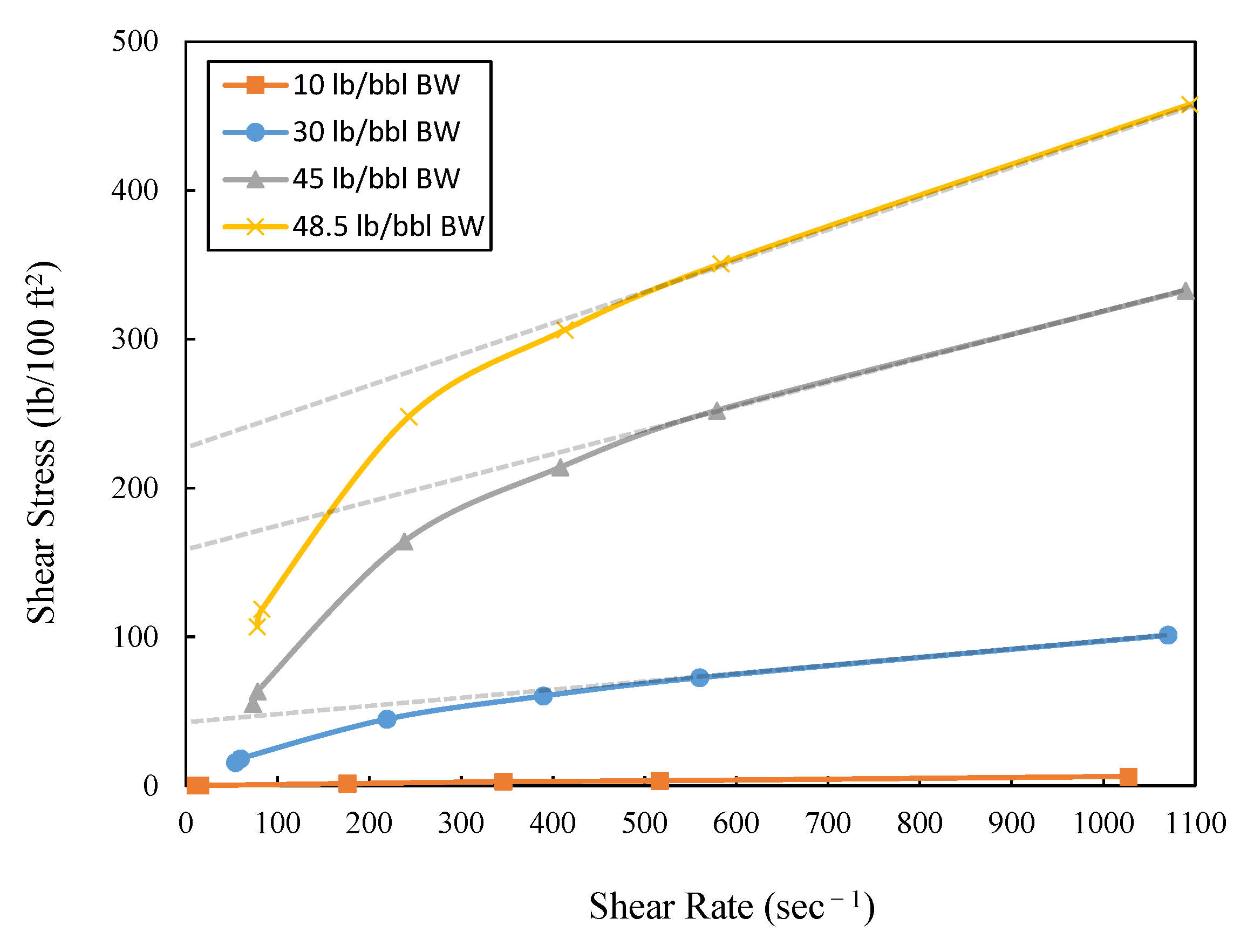
Figure A1 displays the measured shear-stress/shear-rate relationship for the fluids used in this study. All data were measured using a Fann 35 rotational viscometer at rotational speeds of 3, 6, 100, 200, 300 and 600 rpm. The dotted line y-axis intercept for each fluid represents its theoretical yield point, τy, for a Bingham plastic fluid. The curves for 30, 45 and 48.5 lb/bbl BW mixtures, at initial inspection, suggest that τy does not actually represent a physical characteristic of these fluids. This intuitive conclusion, however, would not be correct. Under the dynamic conditions of a rotational viscometer, the low-shear-rate behavior shown below is common for a bentonite–water mixture. However, under static conditions, bentonite particles quickly build a gel structure that results in an actual τy reasonably approximated by the theoretical Bingham plastic τy. Thus, the yield point of a fluid is certainly a meaningful physical characteristic for understanding Taylor bubble behavior under static fluid conditions, and the shear stresses observed at low shear rates are material to dynamic fluid conditions. Considering that both static and dynamic fluid conditions play a role in this analysis, our method for estimating apparent viscosity based on a Bingham plastic model is a reasonable tool for use in our correlation. Furthermore, our preference for using the theoretical Bingham Plastic τy instead of a measured τy in our analysis stems from the difficulty of obtaining consistent ultra-low-shear measurements for high-viscosity fluids. The theoretical Bingham Plastic τy is an easier-to-use and more consistent proxy for direct τy laboratory measurements.
Figure A1.
Shear stress against shear rate.

References
- Evje, S.; Fjelde, K.K. Hybrid Flux-Splitting Schemes for a Two-Phase Flow Model. J. Comput. Phys. 2002, 175, 674–701. [Google Scholar] [CrossRef]
- Fabre, J.; Figueroa-Espinoza, B. Taylor bubble rising in a vertical pipe against laminar or turbulent downward flow: Symmetric to asymmetric shape transition. J. Fluid Mech. 2014, 755, 485–502. [Google Scholar] [CrossRef] [Green Version]
- Fershtman, A.; Babin, V.; Barnea, D.; Shemer, L. On shapes and motion of an elongated bubble in downward liquid pipe flow. Phys. Fluids 2017, 29, 112103. [Google Scholar] [CrossRef]
- Kelessidis, V.C.; Dukler, A. Motion of large gas bubbles through liquids in vertical concentric and eccentric annuli. Int. J. Multiph. Flow 1990, 16, 375–390. [Google Scholar] [CrossRef]
- Daş, G.; Das, P.; Purohit, N.; Mitra, A. Rise velocity of a Taylor bubble through concentric annulus. Chem. Eng. Sci. 1998, 53, 977–993. [Google Scholar] [CrossRef]
- Agarwal, V.; Jana, A.K.; Daş, G.; Das, P.K. Taylor bubbles in liquid filled annuli: Some new observations. Phys. Fluids 2007, 19, 108105. [Google Scholar] [CrossRef]
- Lei, Q.; Xie, Z.; Pavlidis, D.; Salinas, P.; Veltin, J.; Matar, O.K.; Pain, C.C.; Muggeridge, A.H.; Gyllensten, A.J.; Jackson, M.D. The shape and motion of gas bubbles in a liquid flowing through a thin annulus. J. Fluid Mech. 2018, 855, 1017–1039. [Google Scholar] [CrossRef]
- Nicklin, D.J. Two-phase flow in vertical tubes. Trans. Inst. Chem. Eng. 1962, 40, 61–68. [Google Scholar]
- Choi, J.; Pereyra, E.; Sarica, C.; Park, C.; Kang, J.M. An Efficient Drift-Flux Closure Relationship to Estimate Liquid Holdups of Gas-Liquid Two-Phase Flow in Pipes. Energies 2012, 5, 5294–5306. [Google Scholar] [CrossRef] [Green Version]
- Bhagwat, S.M.; Ghajar, A.J. A flow pattern independent drift flux model based void fraction correlation for a wide range of gas–liquid two phase flow. Int. J. Multiph. Flow 2014, 59, 186–205. [Google Scholar] [CrossRef]
- Tang, H.; Bailey, W.; Stone, T.; Killough, J. A Unified Gas-Liquid Drift-Flux Model for Coupled Wellbore-Reservoir Simulation. In Proceedings of the SPE Annual Technical Conference and Exhibition, Calgary, AB, Canada, 30 September–2 October 2019. [Google Scholar]
- Liu, Y.; Tong, T.A.; Ozbayoglu, E.; Yu, M.; Upchurch, E. An improved drift-flux correlation for gas-liquid two-phase flow in hori-zontal and vertical upward inclined wells. J. Pet. Sci. Eng. 2020, 195, 107881. [Google Scholar] [CrossRef]
- Dumitrescue, D.T. Strömung an einer Luftblase im senkrechten Rohr. ZAMM 1943, 23, 139–149. [Google Scholar] [CrossRef]
- Davies, R.M.; Taylor, G.I. The mechanics of large bubbles rising through extended liquids and through liquids in tubes. In Proceedings of the Royal Society of London. Series A. Mathematical and Physical Sciences; The Royal Society: London, UK, 1950; Volume 200, pp. 375–390. [Google Scholar]
- Viana, F.; Pardo, R.; Yánez, R.; Trallero, J.L.; Joseph, D.D. Universal correlation for the rise velocity of long gas bubbles in round pipes. J. Fluid Mech. 2003, 494, 379–398. [Google Scholar] [CrossRef] [Green Version]
- Morgado, A.O.; Miranda, J.M.; Araújo, J.D.; Campos, J.B. Review on vertical gas–liquid slug flow. Int. J. Multiph. Flow 2016, 85, 348–368. [Google Scholar] [CrossRef]
- Bendiksen, K.H. An experimental investigation of the motion of long bubbles in inclined tubes. Int. J. Multiph. Flow 1984, 10, 467–483. [Google Scholar] [CrossRef] [Green Version]
- Hasan, A.R.; Kabir, C.S. Predicting Multiphase Flow Behavior in a Deviated Well. SPE Prod. Eng. 1988, 3, 474–482. [Google Scholar] [CrossRef]
- Gokcal, B.; Al-Sarkhi, A.; Sarica, C. Effects of High Oil Viscosity on Drift Velocity for Horizontal and Upward Inclined Pipes. SPE Proj. Facil. Constr. 2009, 4, 32–40. [Google Scholar] [CrossRef]
- Benjamin, T.B. Gravity currents and related phenomena. J. Fluid Mech. 1968, 31, 209–248. [Google Scholar] [CrossRef]
- Jeyachandra, B.C.; Gokcal, B.; Al-Sarkhi, A.; Sarica, C.; Sharma, A.K. Drift-Velocity Closure Relationships for Slug Two-Phase High-Viscosity Oil Flow in Pipes. SPE J. 2012, 17, 593–601. [Google Scholar] [CrossRef]
- Moreiras, J.; Pereyra, E.; Sarica, C.; Torres, C.F. Unified drift velocity closure relationship for large bubbles rising in stagnant vis-cous fluids in pipes. J. Pet. Sci. Eng. 2014, 124, 359–366. [Google Scholar] [CrossRef]
- Lizarraga-Garcia, E.; Buongiorno, J.; Al-Safran, E.; Lakehal, D. A broadly-applicable unified closure relation for Taylor bubble rise velocity in pipes with stagnant liquid. Int. J. Multiph. Flow 2017, 89, 345–358. [Google Scholar] [CrossRef] [Green Version]
- Carew, P.; Thomas, N.; Johnson, A. A physically based correlation for the effects of power law rheology and inclination on slug bubble rise velocity. Int. J. Multiph. Flow 1995, 21, 1091–1106. [Google Scholar] [CrossRef]
- Majumdar, A.; Das, P.K. Rise of Taylor bubbles through power law fluids–Analytical modelling and numerical simulation. Chem. Eng. Sci. 2019, 205, 83–93. [Google Scholar] [CrossRef]
- Shosho, C.E.; Ryan, M.E. An experimental study of the motion of long bubbles in inclined tubes. Chem. Eng. Sci. 2001, 56, 2191–2204. [Google Scholar] [CrossRef]
- Kamışlı, F. Free coating of a non-Newtonian liquid onto walls of a vertical and inclined tube. Chem. Eng. Process. Process Intensif. 2003, 42, 569–581. [Google Scholar] [CrossRef]
- Sousa, R.; Riethmuller, M.; Pinto, A.; Campos, J.B.L.M. Flow around individual Taylor bubbles rising in stagnant CMC solutions: PIV measurements. Chem. Eng. Sci. 2005, 60, 1859–1873. [Google Scholar] [CrossRef] [Green Version]
- Sousa, R.G.; Riethmuller, M.; Pinto, A.; Campos, J.B.L.M. Flow around individual Taylor bubbles rising in stagnant polyacrylamide (PAA) solutions. J. Non-Newtonian Fluid Mech. 2006, 135, 16–31. [Google Scholar] [CrossRef]
- Rabenjafimanantsoa, A.H.; Time, R.W.; Paz, T. Dynamics of expanding slug flow bubbles in non-Newtonian drilling fluids. Ann. Trans. Nord. Rheol. Soc. 2011, 19, 1–8. [Google Scholar]
- Araújo, J.D.P.; Miranda, J.M.; Campos, J.B.L.M. Taylor bubbles rising through flowing non-Newtonian inelastic fluids. J. Non-Newtonian Fluid Mech. 2017, 245, 49–66. [Google Scholar] [CrossRef]
- Griffith, P.; Wallis, G.B. Two-Phase Slug Flow. J. Heat Transf. 1961, 83, 307–318. [Google Scholar] [CrossRef]
- Lu, X.; Prosperetti, A. Axial stability of Taylor bubbles. J. Fluid Mech. 2006, 568, 173. [Google Scholar] [CrossRef] [Green Version]
- Ozbayoglu, M.; Kuru, E.; Miska, S.; Takach, N. A Comparative Study of Hydraulic Models for Foam Drilling. J. Can. Pet. Technol. 2002, 41. [Google Scholar] [CrossRef]
- Ozbayoglu, M.E.; Miska, S.Z.; Reed, T.; Takach, N. Analysis of the effects of major drilling parameters on cuttings transport effi-ciency for high-angle wells in coiled tubing drilling operations. In Proceedings of the SPE/ICoTa Coiled Tubing Conference and Exhibition, Houston, TX, USA, 23–24 March 2004. [Google Scholar]
- Liu, Y.; Luo, C.; Zhang, L.; Liu, Z.; Xie, C.; Wu, P. Experimental and modeling studies on the prediction of liquid loading onset in gas wells. J. Nat. Gas Sci. Eng. 2018, 57, 349–358. [Google Scholar] [CrossRef]
- Tong, T.A.; Liu, Y.; Ozbayoglu, E.; Yu, M.; Ettehadi, R.; May, R. Threshold velocity of non-Newtonian fluids to initiate solids bed erosion in horizontal conduits. J. Pet. Sci. Eng. 2021, 199, 108256. [Google Scholar] [CrossRef]
- Dadashev, R.K.; Mezhidov, V.K.; Dzhambulatov, R.S.; Elimkhanov, D.Z. Features of isotherms of the surface tension of a bentonite water suspension. Bull. Russ. Acad. Sci. Phys. 2014, 78, 288–290. [Google Scholar] [CrossRef]
- Bourgoyne, A.T., Jr.; Millheim, K.K.; Chenevert, M.E.; Young, F.S., Jr. Applied Drilling Engineering; Society of Petroleum Engineers: Richardson, TX, USA, 1991. [Google Scholar]
- Zukoski, E.E. Influence of viscosity, surface tension, and inclination angle on motion of long bubbles in closed tubes. J. Fluid Mech. 1966, 25, 821–837. [Google Scholar] [CrossRef] [Green Version]
- Tong, T.A.; Yu, M.; Ozbayoglu, E.; Takach, N. Numerical simulation of non-Newtonian fluid flow in partially blocked eccentric annuli. J. Pet. Sci. Eng. 2020, 193, 107368. [Google Scholar] [CrossRef]
- Luo, C.; Zhang, L.; Liu, Y.; Zhao, Y.; Xie, C.; Wang, L.; Wu, P. An improved model to predict liquid holdup in vertical gas wells. J. Pet. Sci. Eng. 2020, 184, 106491. [Google Scholar] [CrossRef]
- Eghorieta, R.A.; Pugliese, V.; Panacharoensawad, E. Experimental and Numerical Studies on the Drift Velocity of Two-Phase Gas and High-Viscosity-Liquid Slug Flow in Pipelines. In Proceedings of the Offshore Technology Conference, Houston, TX, USA, 6–9 May 2019. [Google Scholar]
- Livinus, A.; Verdin, P.; Lao, L.; Nossen, J.; Langsholt, M.; Sleipnæs, H.G. Simplified generalised drift velocity correlation for elon-gated bubbles in liquid in pipes. J. Pet. Sci. Eng. 2018, 160, 106–118. [Google Scholar] [CrossRef] [Green Version]
- Zuber, N.; Findlay, J.A. Average Volumetric Concentration in Two-Phase Flow Systems. J. Heat Transf. 1965, 87, 453–468. [Google Scholar] [CrossRef]
Figure 1.
General view and schematic view of the experimental facility.

Figure 2.
Buffer accumulator and air valve. (A1: release the air under static condition; A2, A3, and A4: release the air under countercurrent flow condition).
Figure 2.
Buffer accumulator and air valve. (A1: release the air under static condition; A2, A3, and A4: release the air under countercurrent flow condition).

Figure 3.
Pump connection (a) and mud return (b).

Figure 4.
Flow rig built for this study.

Figure 5.
Instruments positioned along the test section.

Figure 6.
Determination of the velocity and length of Taylor bubble.

Figure 7.
Differential pressure to determine the velocity of Taylor bubbles.

Figure 8.
Differential pressure to determine the length of Taylor bubble. (a) The length of the Taylor bubble is shorter than the distance of two pressure transducers; (b) the length of the Taylor bubble is larger than the distance between two pressure transducers.
Figure 8.
Differential pressure to determine the length of Taylor bubble. (a) The length of the Taylor bubble is shorter than the distance of two pressure transducers; (b) the length of the Taylor bubble is larger than the distance between two pressure transducers.

Figure 9.
Drift velocity as a function of inclination angle.

Figure 10.
Air–liquid mixture density (ρm) change with time at 45° from vertical. (a) 10 lb/bbl BW; (b) 30 lb/bbl BW; (c) 45 lb/bbl BW; (d) 48.5 lb/bbl BW.
Figure 10.
Air–liquid mixture density (ρm) change with time at 45° from vertical. (a) 10 lb/bbl BW; (b) 30 lb/bbl BW; (c) 45 lb/bbl BW; (d) 48.5 lb/bbl BW.

Figure 11.
Influence of apparent viscosity on drift velocity (data set in Appendix A).
Figure 11.
Influence of apparent viscosity on drift velocity (data set in Appendix A).

Figure 12.
Performance of the proposed correlation for predicting drift velocity (dataset in Appendix A).
Figure 12.
Performance of the proposed correlation for predicting drift velocity (dataset in Appendix A).

Figure 13.
The performance of the proposed correlation against a database of other investigator’s results (using both Newtonian and non-Newtonian fluids).
Figure 13.
The performance of the proposed correlation against a database of other investigator’s results (using both Newtonian and non-Newtonian fluids).

Figure 14.
Influence of on . (a) Water; (b) 45 lb/bbl BW; (c) 48.5 lb/bbl BW.

Figure 15.
Influence of liquid viscosity on . (a) = 0.218 m/s; (b) = 0.5 m/s.

Figure 16.
against the inclination angles. (a) Water; (b) Bingham plastic fluid.

Figure 17.
Flow profile between a Newtonian fluid and non-Newtonian fluid.

Figure 18.
Influence of and on the in water.

Figure 19.
Dimensionless bubble length () as a function of . (a) Water volume 1; (b) water volume 2; (c) 45 lb/bbl BW; (d) 48.5 lb/bbl BW.
Figure 19.
Dimensionless bubble length () as a function of . (a) Water volume 1; (b) water volume 2; (c) 45 lb/bbl BW; (d) 48.5 lb/bbl BW.

Figure 20.
Influence of liquid viscosity on the . (a) = 0.218 m/s; (b) = 0.5 m/s.

Figure 21.
Gel strength caused a stagnant Taylor bubble in 48.5 lb/bbl BW at 4°.

Figure 22.
Drift velocity at different position of the pipe. (a) 10 lb/bbl BW; (b) 30 lb/bbl BW; (c) 45 lb/bbl BW; (d) 48.5 lb/bbl BW.
Figure 22.
Drift velocity at different position of the pipe. (a) 10 lb/bbl BW; (b) 30 lb/bbl BW; (c) 45 lb/bbl BW; (d) 48.5 lb/bbl BW.

Figure 23.
as a function of for 48.5 lb/bbl BW at 4°.

Table 1.
Physical properties and test matrix.
| Liquid | Condition | ID (m) | (°) | (kg/m3) | (cp) | (lb/100 ft2) | (m/s) | |
|---|---|---|---|---|---|---|---|---|
| Water | S/C | 0.1524 | 4, 15, 30, 45 | 998 | 1 | - | 0.173~0.7 | 26,306~105,227 |
| 10 lb/bbl BW | S | 0.1524 | 4, 15, 30, 45 | 1014 | 2.4 | 0.75 | 0 | - |
| 30 lb/bbl BW | S | 0.1524 | 4, 15, 30, 45 | 1047 | 27 | 41.6 | 0 | - |
| 45 lb/bbl BW | S/C | 0.1524 | 4, 15, 30, 45 | 1063 | 76 | 162 | 0.22~0.7 | 477~1113 |
| 48.5 lb/bbl BW | S/C | 0.1524 | 4, 15, 30, 45 | 1076 | 101 | 230 | 0.073~0.7 | 118~803 |
1 Plastic viscosity () is defined as ; 2 Yield point was obtained by , where and are the dial readings at 600 rpm and 300 rpm, respectively, using a Fann 35 rotational viscometer with an R1B1 bob (using F1 and F2 springs as appropriate); 3 Reynolds number () is defined as [39].
Table 2.
The quantitative performance of different correlations against experimental data.
| Correlations | 15% | 10% | Statistical Parameter | ||
|---|---|---|---|---|---|
| Bendiksen | 42.10% | 21.05% | 0.06619 | 0.3391 | 0.1782 |
| Hasan and Kabir | 5.26% | 0.00% | −0.247 | 0.5575 | 0.2242 |
| Gokcal | 57.89% | 36.84% | 0.1079 | 0.35831 | 0.1988 |
| Jeyachandra | 47.37% | 42.10% | 0.1465 | 0.3903 | 0.2132 |
| Moreiras | 21% | 16% | 0.02351 | 0.3078 | 0.1622 |
| Lizarraga-Garcia | 31.58% | 10.53% | −0.03655 | 0.2907 | 0.1628 |
| Proposed correlation | 90% | 80% | 0.00201 | 0.0702 | 0.093 |
Table 3.
Sources and properties of the database used for correlation validation.
| Source | Fluids | Pipe Diameter (mm) | Inclination Angle (°) | n | k | |
|---|---|---|---|---|---|---|
| Carew et al. | Carbopol 981 | 25, 45, 70 | 0 | - | 0.386, 0.485 | 1.016, 2.927 |
| Sousa et al. | CMC | 32 | 0 | - | 0.437~0.772 | 0.079~4.189 |
| Eghorieta et al. | Water | 50.8 | 80, 83, 85, 87, 89, 90 | 0.001 | - | - |
| Livinus et al. | Oil | 57, 99 | 82.5, 85, 87.5, 89 | 0.16, 1.14 | - | - |
Publisher’s Note: MDPI stays neutral with regard to jurisdictional claims in published maps and institutional affiliations. |
© 2021 by the authors. Licensee MDPI, Basel, Switzerland. This article is an open access article distributed under the terms and conditions of the Creative Commons Attribution (CC BY) license (http://creativecommons.org/licenses/by/4.0/).
Share and Cite
MDPI and ACS Style
Liu, Y.; Upchurch, E.R.; Ozbayoglu, E.M. Experimental Study of Single Taylor Bubble Rising in Stagnant and Downward Flowing Non-Newtonian Fluids in Inclined Pipes. Energies 2021, 14, 578. https://doi.org/10.3390/en14030578
AMA Style
Liu Y, Upchurch ER, Ozbayoglu EM. Experimental Study of Single Taylor Bubble Rising in Stagnant and Downward Flowing Non-Newtonian Fluids in Inclined Pipes. Energies. 2021; 14(3):578. https://doi.org/10.3390/en14030578
Chicago/Turabian StyleLiu, Yaxin, Eric R. Upchurch, and Evren M. Ozbayoglu. 2021. "Experimental Study of Single Taylor Bubble Rising in Stagnant and Downward Flowing Non-Newtonian Fluids in Inclined Pipes" Energies 14, no. 3: 578. https://doi.org/10.3390/en14030578
Note that from the first issue of 2016, this journal uses article numbers instead of page numbers. See further details here.