Point and Interval Forecasting of Zonal Electricity Prices and Demand Using Heteroscedastic Models: The IPEX Case

Abstract

Since the electricity market liberalisation of the mid-1990s, forecasting energy demand and prices in competitive markets has become of primary importance for energy suppliers, market regulators and policy makers. In this paper, we propose a non-parametric model to obtain point and interval predictions of price and demand. It does not require any parametric assumption on the distribution of the error term or on the functional relationships linking the response variable to covariates. The assumed location–scale model provides a non-parametric estimation of the conditional mean and of the conditional variance by means of a Generalised Additive Model. Interval forecasts, at any given confidence level, are then obtained using a further non-parametric estimation of the innovation’s quantile. Since both the conditional mean and the conditional variance of the response variable are non-linear functions of covariates depending on calendar factors, renewable energy productions and other market variables, the resulting model is very flexible. It easily adapts to market conditions as well as to the non-linear characteristics of demand, supply and prices. An application to hourly data for the Italian electricity market, over the period 2015–2019 period, shows the one-day-ahead forecasting performance of the model for zonal electricity prices and level of demand.

1. Introduction

Electricity market variables forecasting is of great economic and environmental importance and, indirectly, provides benefits for the entire economy. Accurate electricity power load and price predictions are important to utility companies for their daily activities and future planning and to market operators and investors in the decision making processes. They are also useful for market actors and transmission system operators (TSO) in scheduling production activity and avoiding temporary electrical power failures (see, e.g., [1,2]). Moreover, electricity market liberalisation greatly enhanced the level of competition in electricity markets asking for more accurate demand and price predictions. To meet the increasing demand for new and more sophisticated forecasting methodologies, over the last few decades, a number of methods and ideas with varying degrees of novelty and success, were developed, (see, e.g., [3] for a recent overview of forecasting methods). As indicated by several authors ([4,5] among others), electricity time series exhibit a complex behaviours characterised by non-linear time and cross-sectional dependence, heteroscedasticity, multiple seasonal cycles, extreme spikes, kurtosis and, sometimes, outliers. Moreover, both prices and loads depend—possibly non-linearly—on other exogenous market variables, including renewable energy productions.

Nevertheless, until recently, models proposed in the literature have mainly dealt with complex seasonal cycles within a time series approach. They include Holt–Winters exponential smoothing methods, seasonal autoregressive integrated moving average (SARIMA) model (see, e.g., [6,7,8,9,10,11,12,13,14,15]), linear regression models [16] and any combination thereof [17,18]. Ref. [8] considered a reasonable improvement in the existing exponential smoothing methods introducing a double seasonal exponential smoothing approach, as well as seasonal ARIMA models. The limit of this approach is that the same intra-daily cycle is assumed to hold for all days of the week. Ref. [12] proposed a new approach, based on state-space models, to forecast time series with multiple innovation patterns. To avoid the need for modelling the intra-daily seasonality of hourly Spanish electricity consumptions, Ref. [19] suggested using individual models for each hour of the day. The same strategy, in a different context, was also suggested by [20]. As an improvement of his previous work, Ref. [9,10] proposed a triple seasonal model, which was able to describe intra-day, intra-week and intra-year cycles. With specific reference to the Italian electricity market, Ref. [18] recently considered long memory heteroscedastic linear regression models to investigate the impact of new technological developments, market concentration, congestion and volume on zonal price dynamics, while [21], after a deep empirical analysis of the characteristics of the Italian market, mainly focused on the relevant issue of market congestion and interdependency of Italian zonal prices. Ref. [22] provided a survey of state-of-the-art electricity price forecasting, focusing on three broad classes of models: autoregressive, regime-switching, and conditional volatility models. They concluded their empirical analysis by arguing that, among the stylised facts regarding electricity markets, the lack of clear-cut evidence for a specific analytical framework is the most peculiar, favouring the development of new semi-parametric methods. To take into account such issues, they proposed the adoption of time-varying parameters dynamic factor models. Comprehensive and up-to-date reviews of energy load and prices forecasting techniques are given, respectively, in [1,4,23,24].

In reviewing some of the main methodological issues and techniques for short-term forecasting of loads and prices, Ref. [20] recommendes non-linear models such as neural networks and forecast combinations, as a way to exploit predictive information provided by different models. Combining forecasts is also the focus of the work of [25]. Ref. [26], in a recent survey, presented a detailed analysis for the structural approach for electricity modelling, emphasising its merits with respect to traditional reduced-form models. Although several recent works advocate a broad and flexible structural framework for spot prices, incorporating demand, capacity and fuel prices in several ways, this approach was neglected, until recently.

The fast development of electricity markets along with their complexity and the overall level of competition among operators recently stimulated significant interest in probabilistic forecasting (see, e.g., [4]). Probabilistic forecasting involves computing quantiles, intervals or the whole predictive density rather than simple point predictions based on the conditional mean. As pointed out by [27], the probabilistic approach serves several purposes such as stochastic unit commitment, power supply planning, the prediction of equipment failure, and the integration of renewable energy sources, (see, e.g., [28]). The literature on probabilistic electricity forecasting is quite limited [2], particularly compared to that of probabilistic forecasting in general [29] or probabilistic renewable energy forecasting [30,31,32,33]. Ref. [5] recognised that few papers dealing with time series models provide predictive intervals, while forecasting intervals were considered by (e.g., [34,35,36]). In reviewing various statistical and artificial intelligence techniques for energy forecasting, Ref. [37] discussed the factors affecting forecast accuracy such as weather data, time factors, customer classes and economic factors. Moreover, in their discussion about future research directions, the authors pointed out that additional progress in load forecasting and its use in industrial applications could be achieved by providing short-term predictive distributions rather than point forecasts. In this regards, Refs. [2,34] proposed resorting to seasonal autoregressive moving average-generalised autoregressive conditional heteroschedastic (SARMA-GARCH) models, which describe seasonality and other regular and linear behaviours as well as the dynamics of price volatility. Ref. [38] produced predictive intervals by means of cascading neural networks and modified U-D factorisation, respectively, but did not provide any formal assessment of their results. Ref. [39] extended the class of support vector machines to account for heteroscedasticity in the data. Ref. [40] proposed a wavelet-based hybrid neural network for short-term electricity prices forecasting. In an interesting work, Ref. [41] argued for interval forecasting, as a way to describe the uncertainty and reliability of energy price and load point forecasts. To obtain them, he proposed an additive non-parametric model whose location, scale and shape parameters were non-linear additive functions of the covariates. Additive models for conditional expectation were proposed by [42,43] and extended to predict individual quantiles by [44,45]. Linear quantile regression models have also been used by [46], for day-ahead and intra-daily markets, to produce probabilistic forecasts of hourly spot prices with the aim of reducing forecast bias and the width of forecast intervals. Hybrid methods combining a time-series approach with machine learning and data mining techniques were also proposed by the literature on probabilistic forecasting. Ref. [47] compared the Box-Cox transform, ARMA errors, Trend, and Seasonal components (BATS) models and their trigonometric versions (TBATS) of [14], artificial neural networks and seasonal autoregressive methods to predict electricity in the Danish day-ahead market. Ref. [48] described a hybrid approach based on k-means clustering to obtain interval forecasts. A different research stream includes forecasting intervals within a machine-learning approach traditionally used for optimal point forecasts. Within this emerging field, ensemble methods are suggested by [49] and Bayesian deep learning models by [50]. As an evolution of the combination approach used for point forecasts, methods to combine probabilistic density forecasts were also experimented with by [51,52].

All previous considerations and empirical findings asked for more flexible structural approaches to non-linear modelling of complex dependence structures between interacting covariates being enabling the production of accurate point and prediction intervals. The goal of this work is to build reliable interval (or probabilistic) predictions that are able to adapt to the evolving conditions of the electricity market, by modelling the conditional mean and variance as non-parametric functions of suitable covariates. In what follows, we cast the forecasting problem within the wide family of the generalised additive regression model (GAM). This class of models, originally suggested by [53], is widely used in industry and business due to its flexibility and good forecasting results. GAM models are more flexible than standard linear models but, unlike time series models, maintain the interpretability of a general regression surface. The family of additive models for conditional locations were recently enriched by [54] through the inclusion of additive models for the scale and shape parameters of a large class of distributions, including the Gaussian, Student-t, Poisson or Binomial distributions. Within this approach, here we consider a simpler non-parametric location–scale model. Since we are mostly concerned with estimating the functions by modelling conditional mean and variance, model parameters are estimated using quasi-maximum likelihood approach assuming a Gaussian mis-specified likelihood function. Non-parametric prediction intervals are then obtained by adopting a suitable non-parametric bootstrapping procedure [55] for the in-sample standardised residuals. This allows the avoidance of the restrictive assumption of specifying a parametric distribution for the error term, thereby reducing the computational burden without losing too much efficiency and model interpretability. The advantage of this approach over linear regression and pure time series methods is twofold. First, our method easily accounts for multiple seasonal patterns without the need for including additional large-dimensional state variables for the exponential smoothing state space methods (see, e.g., [56]). Moreover, the non-parametric model is flexible enough to adapt to the non-linear effect of seasonal cycles, as well as additional covariates, on the response variable, without losing the structural interpretation of the model parameters. Second, our model accounts for the heteroscedastic nature of the data, thereby adapting the interval forecasts to periods of high and low volatility.

The rest of this paper is structured as follows. Section 2 describes the variables belonging our dataset that relates to the Italian electricity market. Section 3 introduces the semi-parametric heteroscedastic additive regression model and details the parameter estimation via the non-linear back-fitting algorithm. Section 4 shows the output of the model and its interpretation. The forecasting exercise is performed in Section 5, which includes an in-sample analysis to identify the more appropriate models and the out-of-sample forecasting results. Section 6 concludes.

2. The Data

The Italian Power EXchange (IPEX) is divided into portions of the power grid, called Zones, in which for system security purposes, there are physical limits to transfers of electricity to/from other geographical zones. At present, there are six geographical zones: northern Italy, central–northern Italy, central–southern Italy, southern Italy, Sicilia and Sardegna. There are some national virtual zones that are the pole of limited production and some foreign virtual zones, representing points of interconnection with neighbouring countries. In this work we consider only the two main national geographical zones: northern Italy (NORD) and southern Italy (SUD). For these two zones, and for the period 1 January 2015–31 December 2019, the following variables, were available for day t ($t=1,\dots ,n$) and load period (hour) h ($h=1,\dots ,24)$:

-

${\mathsf{P}}_{t,h}$: is the hourly time series of zonal prices, in euros per megawatt-hour (€/MWh), as defined in the Day-Ahead Market (in Italian Mercato del Giorno Prima, MGP). For this market, $P_{t,h}$ is available at time $t-1$;

-

${\mathsf{D}}_{t,h}$: is the hourly time series of the zonal demand for energy (in MWh) as defined in the MGP. Again, as for the price, the demand $D_{t,h}$ ($h=1,\dots ,24$) is available at time $t-1$;

-

${\mathsf{Wind}}_{t,h}$, ${\mathsf{PV}}_{t,h}$, ${\mathsf{Hydro}}_{t,h}$, $\mathsf{Hydro}.{\mathsf{R}}_{t,h}$, ${\mathsf{Therm}}_{t,h}$: represent the hourly time series of, respectively, wind, photovoltaic, hydro from river basins, hydro rivers and thermal energy production (in MWh);

-

${\mathsf{Imp}}_{t,h}$: is the hourly time series of the amount of energy (in MWh) imported from other zones including imports from abroad. This variable is available only for the northern zone;

-

${\mathsf{PSV}}_{t,h}$: denotes the hourly time series of the gas price at the Virtual Trading Point (in Italian Punto di Scambio Virtuale, PSV), for given day $t=1,\dots ,n$ and hour $h=1,\dots ,24$. Since this variable has daily frequency, the hourly time series was obtained by imposing ${\mathsf{PSV}}_{t,h}={\mathsf{PSV}}_t$ for $h=1,\dots ,24$.

In addition to these variables, other calendar variables were used:

-

${\mathsf{trend}}_{t,h}$: represents the “trend” variable or the long–run dynamics on day t. When working with hourly data, we assume that ${\mathsf{trend}}_{t,h}={\mathsf{trend}}_t$, i.e., that the trend variable is constant within a day. This also applies to other variables that have, logically, a daily frequency;

-

${\mathsf{dayyear}}_{t,h}$: represents the yearly periodicity of the data. It is described by a vector repeating the sequence $1,2,\dots ,365\left(366\right)$. For hourly data ${\mathsf{dayyear}}_{t,h}={\mathsf{dayyear}}_t$ for $h=1,\dots ,24$;

-

${\mathsf{dayweek}}_{t,h}$: represents the weekly periodicity of the data. It is described by repeating the periodic sequence $1,\dots ,7$. For hourly data ${\mathsf{dayweekyear}}_{t,h}={\mathsf{dayweek}}_t$ for $h=1,\dots ,24$;

-

${\mathsf{hour}}_{t,h}$: the hour of the day $t=1,2,\dots$, ($h=1,\dots ,24$);

-

${\mathsf{bank}}_{t,h}$: is a dummy variable that accounts for bank holidays assuming a value of 1 if day t is a bank holiday and 0 otherwise. For hourly data ${\mathsf{bank}}_{t,h}={\mathsf{bank}}_t$ for $h=1,\dots ,24$

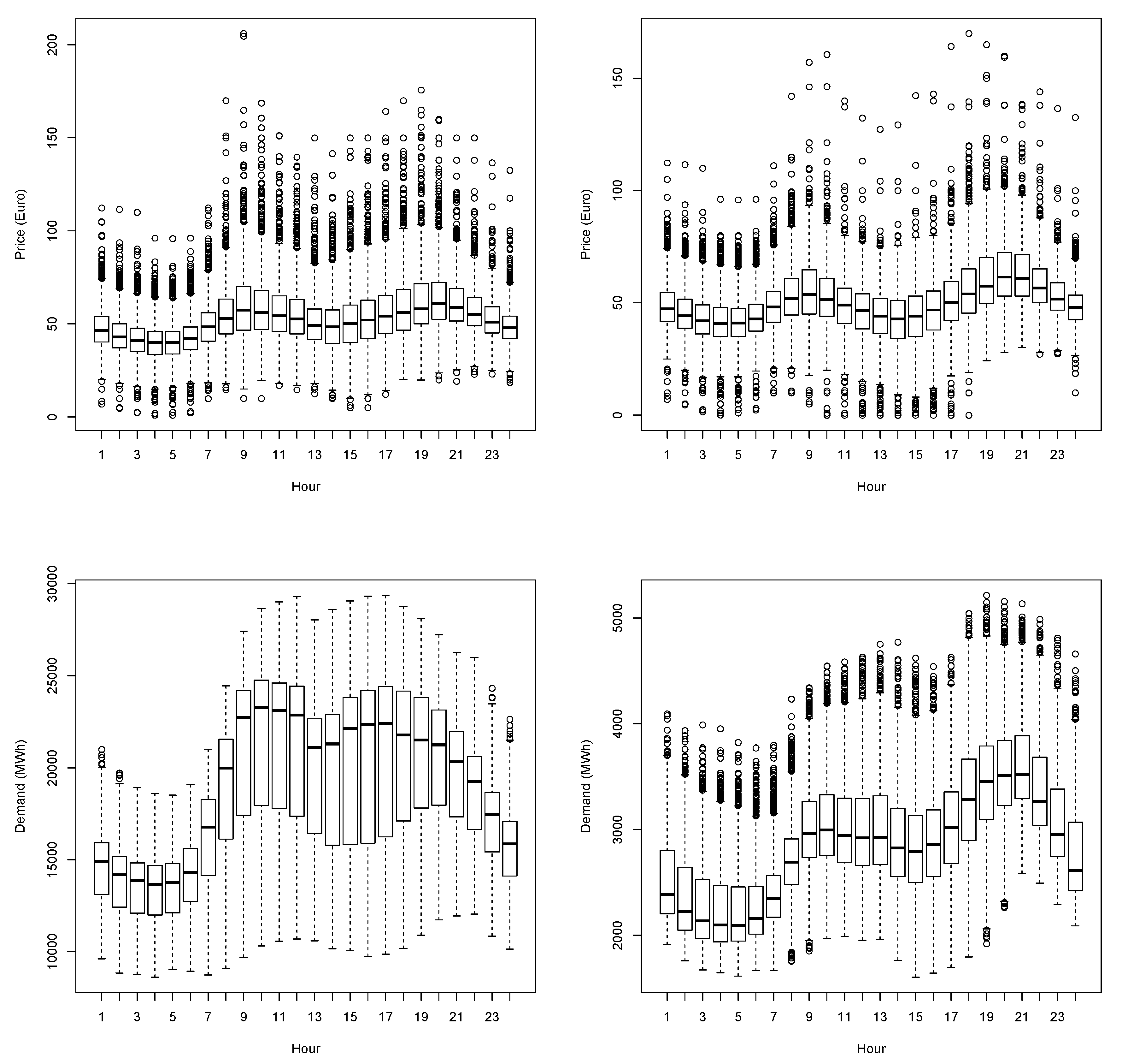
Figure 1 presents boxplots of the variability in prices and demand for the northern and southern zones grouped by the hour of the day (hour) for the years 2015–2019. All reveal a strong daily seasonal pattern as well as the presence of fat-tailed hourly distributions, which are issues well-documented in the literature, (see, e.g., [9,10,11,12,57]). Looking at the scale of the boxplots of demand (bottom panels), it is immediately clear that the northern zone is much more relevant the southern in terms of volume. Indeed, the average electricity production is approximately 15,000 MWh for the northern zone and only about 2500 MWh for the southern one. The strong heterogeneous behaviour in different hours of the day is an additional stylised fact characterising this kind of data. The former empirical evidence is relevant for either the objectives of the present paper and the conclusion of our analyses. Regarding the objectives, the observed heterogeneity motivates the use of semi–parametric heteroscedastic models which will be proposed in the next section. Moreover, since larger volumes reflect in a larger variability of prices and demand data, we expect that flexible semi-parametric models provide better forecasting results than linear or pure time series models for the northern region, where larger volumes might translate into higher benefits to account for the dynamic evolution of the conditional variance.

3. The Semi-Parametric Heteroscedastic Additive Model

Let $y_t$, $(t=1,\dots ,n)$, be a random sample from the random variable $Y_t$, defining the response variable and ${\mathbf{x}}_t=(x_{1,t},\dots ,x_{p,t})$ be a vector of covariates drawn by the p-variate random variable $\mathbf{X}$. Covariates may or may not be exogenous. A heteroscedastic additive regression model assumes the following specification of the dynamics of the response variable $y_t$, conditional on the information available at time t, ${\mathbf{x}}_t$ (or, equivalently, ${\mathcal{I}}_t=\left\{{\mathbf{x}}_s,s\le t\right\}$):

$$\begin{array}{cc}\hfill y_t& =\mu \left({\mathbf{x}}_t\right)+\sigma \left({\mathbf{x}}_t\right)z_t,\hfill \\ \hfill & =\mu \left({\mathbf{x}}_t\right)+{\epsilon }_t,\hfill \end{array}$$

(1)

where the conditional mean and variance are specified by the following non-parametric additive functions:

$$\begin{array}{c}\hfill {\mu }_t\equiv \mu \left({\mathbf{x}}_t\right)={\beta }_0+\sum _{j=1}^p{f}_j\left(x_{j,t}\right)\end{array}$$

(2)

$$\begin{array}{c}\hfill log{\sigma }_t\equiv log\sigma \left({\mathbf{x}}_t\right)={\gamma }_0+\sum _{j=1}^q{h}_j\left(x_{j,t}\right),\end{array}$$

(3)

for $t=1,2,\dots ,n$, where $z_t$ is an independent and identically distributed (i.i.d.) random variable such that, $\mathsf{E}\left(z_t\right)=0$ and $\mathsf{Var}\left(z_t\right)=1$.

Each function $f_j\left(x\right)$ for $j=1,\dots ,p$ in Equation (2) describes the relation between the covariate $x_j$ and the expectation of the response variable $y_t$ conditionally to the values assumed by all other regressors. Likewise, each function $h_j\left(x\right)$ for $j=1,2,\dots ,q$ in Equation (3) represents the relationship between covariate $x_j$ and the logarithm of the variance of $y_t$, conditional on all of the other other variables. Functions $f_j(·)$ and $h_j(·)$ do not have a specific functional form, hence both linear and non-linear specifications are allowed, but they are required to be smooth, i.e., continuous with their first and second derivatives $f_j^{\prime }$ and $f_j^{″}$ (and similarly for $h_j^{\prime }$ and $h_j^{″}$). To avoid problems of model identifiability, we assume that $\mathsf{E}\left(f_j\left(x_j\right)\right)=0$, for $j=1,2,\dots ,p)$. A classical way to non-parametrically approximate the non–linear function $f_j(·)$ is to use spline functions [58]. In this work, in particular, $f_j$ (similarly for $h_j$) is approximated by using smoothing splines, i.e., a minimising function

$$\sum _{t=1}^n{(y_t-f_j\left(x_j\right))}^2+{\lambda }_j\int f_j^{{}^{″}}{\left(x_j\right)}^{2}d{x}_j,$$

(4)

where ${\lambda }_j\in {\mathbb{R}}^{+}$ is a smoothing parameter penalising the irregularity of function $f_j$. It turns out that smoothing splines are natural cubic splines with several knots equal to the number of (different) observations. Function $f_j$ (similarly for $h_j$) is estimated using the back-fitting algorithm originally proposed by [59]. For a dummy variable, function $f_j$ reduces to the standard linear relationship. It is worth noting that, in principle, alternative approximations could be used in place of the smoothing spline approach considered here. For example, Refs. [54,60] in a recent generalised additive model for location, scale and shape (GAMLSS) approach, considered penalised the B-splines of [58], (see also [61]). In this context, where further flexibility is introduced into the variance function, we opt for smoothing splines approximations that require a small number of parameters with respect to P-splines, thereby reducing the computational burden. The smoothing parameter ${\lambda }_j$ is usually estimated using cross-validation methods.

For models (1)–(3) denoted by ${\mathcal{I}}_t=(x_{1,t,h},\dots ,x_{p,t,h})$ the information set up to time t, the point prediction of $y_t$ is the conditional expectation $\mathsf{E}\left(y_t|{\mathcal{I}}_t\right)=\mu \left({\mathbf{x}}_t\right)$, given by expression (2). Of course, for out-of-sample prediction only information up to time $t-1$ can be used hence the conditioning set must be ${\mathcal{I}}_{t-1}$. The variance of $y_t$ conditionally to ${\mathcal{I}}_t$ is

$$\mathsf{Var}\left({\mathsf{y}}_t|{\mathcal{I}}_t\right)=\sigma {\left({\mathbf{x}}_t\right)}^2={\sigma }_t^2=\mathsf{E}\left[{\left(y_t-\mu ({\mathbf{x}}_t\right)}^2|{\mathcal{I}}_t\right]=\mathsf{E}\left({\epsilon }_{t,h}^2|{\mathcal{I}}_t\right).$$

(5)

As ${\epsilon }_{t,h}$ is assumed to have a zero mean, the conditional variance of $y_t$ coincides with the conditional variance of ${\epsilon }_{t,h}$, which can be estimated using a non-parametric regression of ${\epsilon }_t^2$ on ${\mathbf{x}}_t$.

For our location-scale model, the estimation of the conditional variance allows obtaining prediction intervals at the $(1-\alpha )$ significance level, which can be written as follows:

$$\left[\mu \left({\mathbf{x}}_t\right)+q_z(\alpha /2)·\sigma \left({\mathbf{x}}_t\right);\mu \left({\mathbf{x}}_t\right)+q_z(1-\alpha /2)·\sigma \left({\mathbf{x}}_t\right)\right],$$

(6)

where $q_z\left(\alpha \right)$ is the $\alpha$-quantile of innovation $z_t$.

It is well-known that the electricity market time series includes several components describing long-term dynamics, yearly, weekly and daily periodicities and calendar effects, such as bank holidays. Moreover, the time series of electricity prices might also depend on demand, on production from renewable sources, on the price of other fuels, such as gas, as well as, on the quantity of energy imported from abroad. To account for the previous features and following the approach of [62,63], we use the previously described model to describe the hourly dynamics of electricity price, ${\mathsf{P}}_{t,j}$ (likewise for demand, ${\mathsf{D}}_{t,j}$). The term “additive” means that joint effects between the variables are not considered. Referring to the variables described in Section 2, the specification of the model for the conditional mean is as follows:

$$\begin{array}{cc}\hfill {\mu }_{t,h}& ={\beta }_0+f_1\left({\mathsf{trend}}_{t,h}\right)+f_2\left({\mathsf{dayyear}}_{t,h}\right)+f_3\left({\mathsf{dayweek}}_{t,h}\right)+f_4\left({\mathsf{hour}}_{t,h}\right)\hfill \\ \hfill & +{\mathsf{bank}}_t+f_5\left({\mathsf{Wind}}_{t,h}\right)+f_6\left({\mathsf{PV}}_{t,h}\right)+f_7\left({\mathsf{Hydro}}_{t,h}\right)\hfill \\ \hfill & +f_8(\mathsf{Hydro}.{\mathsf{R}}_{t,h})+f_9\left({\mathsf{Therm}}_{t,h}\right)+f_{10}\left({\mathsf{Imp}}_{t,h}\right)+f_{11}\left({\mathsf{D}}_{t,h}\right)\hfill \\ \hfill & +f_{12}\left({\mathsf{PSV}}_{t,h}\right)+f_{13}\left({\mathsf{P}}_{t-1,h}\right),\hfill \end{array}$$

(7)

for hour $h=1,\dots ,24$ of day $t=1,\dots$. The additive model specified in Equation (7) accounts for the long-run dynamics of electricity demand and prices by the non-parametric function of the time $f_1\left({\mathsf{trend}}_{t,h}\right)$ but also considers several periodic components having different frequencies, yearly $f_2\left({\mathsf{dayyear}}_{t,h}\right)$, weekly $f_3\left({\mathsf{dayweek}}_{t,h}\right)$ and hourly $f_4\left({\mathsf{hour}}_{t,h}\right)$ that usually characterise electricity demand and price data (see, e.g., [9,47]). In general, the calendar effects included depend on the market; here we consider only the bank holiday effect, which is accounted for by the inclusion of the dummy variable ${\mathsf{bank}}_{t,h}$, which is assumed to linearly impact either electricity demand or prices. It is worth noting that model (7) explicitly contains the variable ${\mathsf{hour}}_{t,h}$ to account for the daily periodicity. Another way to treat this component, often used in the literature, is to separately model the daily series of each given hour of the day. This leads to a drop in the function $f_4\left(hou{r}_{t,h}\right)$ and the need to estimate 24 models, one for each load period. In the first part of the paper we use the former approach but later, for out-of-sample prediction, the latter is used.

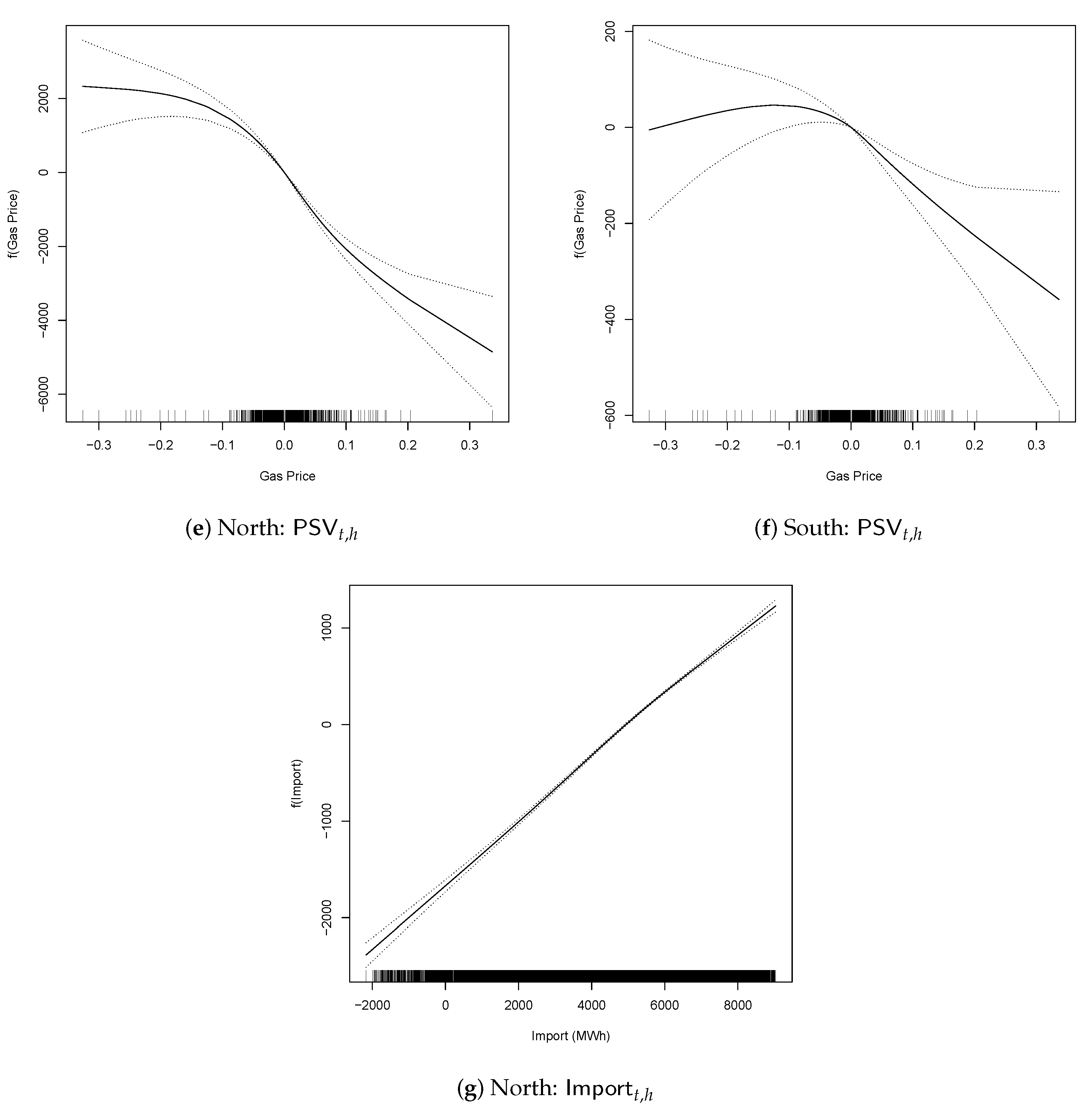
One of the main goals of the model specified in Equation (7) is to assess the impact of the production of renewable energy sources and their uncertainty on point and interval forecasts of electricity prices and demand. Therefore, Equation (7) includes the non-linear contribution of renewable sources such as wind power (${\mathsf{Wind}}_{t,h}$), solar $\left({\mathsf{PV}}_{t,h}\right)$, geothermal $\left({\mathsf{Therm}}_{t,h}\right)$, hydro $\left({\mathsf{Hydro}}_{t,h}\right)$ and hydro river $\left({\mathsf{HydroR}}_{t,h}\right)$. We also expect that the amount of electricity loaded from abroad $\left({\mathsf{Imp}}_{t,h}\right)$ might impact the conditional mean of electricity prices, at least for the northern region of Italy. The last few covariates are electricity load $\left({\mathsf{D}}_{t,h}\right)$, gas prices $\left({\mathsf{PSV}}_{t,h}\right)$ and the level of the electricity price the day before $\left({\mathsf{P}}_{t-1,h}\right)$ to account for short-term dependencies among prices.

For the semi–parametric heteroscedastic additive model the specification of the conditional variance is given by

$$\begin{array}{cc}\hfill \begin{array}{c}\hfill {\sigma }_{t,h}^2\end{array}& =exp\left\{{\gamma }_0+h_1\left({\mathsf{trend}}_{t,h}\right)+h_2\left({\mathsf{dayyear}}_{t,h}\right)+h_3\left({\mathsf{dayweek}}_{t,h}\right)+h_4\left({\mathsf{hour}}_{t,h}\right)\right.\hfill \\ \hfill & +{\mathsf{bank}}_t+h_5\left({\mathsf{Wind}}_{t,h}\right)+h_6\left({\mathsf{PV}}_{t,h}\right)+h_7\left({\mathsf{Hydro}}_{t,h}\right)\hfill \\ \hfill & +h_8(\mathsf{Hydro}.{\mathsf{R}}_{t,h})+h_9\left({\mathsf{Therm}}_{t,h}\right)+h_{10}\left({\mathsf{Imp}}_{t,h}\right)+h_{11}\left({\mathsf{D}}_{t,h}\right)\hfill \\ \hfill & \left.+h_{12}\left({\mathsf{PSV}}_{t,h}\right)+h_{13}\left({\mathsf{P}}_{t-1,h}\right)\right\},\hfill \end{array}$$

(8)

for hour $h=1,2,\dots ,24$ of day $t=1,2,\dots$.

In this work, the model for the conditional mean is always the same but different models and specifications are considered for the conditional variance $\mathsf{Var}\left({\mathsf{P}}_{t,h}|{\mathcal{I}}_t\right)$ (likewise for ${\mathsf{D}}_{t,h}$). In particular, the conditional variance is modelled by assuming:

(i) 

the homoscedasticity of the error term that assumes $\mathsf{Var}\left({\mathsf{P}}_{t,h}\right|{\mathcal{I}}_t)={\sigma }^2$, for each $(t,h)$;

(ii) 

a parametric dynamic evolution. Within this approach we assume that the error term ${\epsilon }_{t,h}$ in Equation (1) follows the GARCH process (see, e.g., [64,65])

$$\mathsf{Var}\left({\mathsf{P}}_{t,h}\right|{\mathcal{I}}_t)=\mathsf{Var}\left({\epsilon }_{t,h}^2\right|{\mathcal{I}}_t)={\sigma }_{t,h}^2=\omega +\alpha {\epsilon }_{t-1,h}^2+\beta {\sigma }_{t-1,h}^2,$$

(9)

with the usual assumptions on the parameters $\omega >0$, $\alpha ,\beta \ge 0$ as well as the condition $\alpha +\beta <1$ that preserves the existence of a weakly stationary solution. Since this approach is fully parametric, two different probability distributions of innovation $z_t$ are considered: the Gaussian and the Student-t. The GARCH parameters were estimated by means of the maximum likelihood method, (see, e.g., [65]).

(iii) 

the non-parametric model (8). In this case, to assure the positivity of the conditional variance, function $h_j$ was estimated using a non-parametric regression of $log\left({\epsilon }_{t,h}^2\right)$ on suitable covariates, where the additional non-parametric function $h_{14}\left(log\left({\epsilon }_{t-1,h}^2\right)\right)$ of past log-squared errors was introduced to account for a possible serial dependence in the time series. Within this class, we consider a model whose conditional variance depends on all of the available variables, called the Full–GAM model, and a model whose conditional variance exploits only the calendar variables. We call the latter Calendar–GAM model. In the non-parametric case, we do not make any distributional assumptions on $z_t$, thus, to estimate quantile $q_z\left(\alpha \right)$ we use the empirical quantile of the variable ${\widehat{z}}_t=(y_t-{\widehat{\mu }}_t)/{\widehat{\sigma }}_t$. This make our approach fully non-parametric.

It is clear that not all of the variables in Equations (7) and (8) will be statistically significant: some are always not significant while others are significant only for some Load Periods. Moreover, in the following analysis, the sentence “the variable is non-significant” will be used with the meaning that the contribution given by the spline of that variable to the reduction of the residual deviance of the model is too small, in the sense of an ANOVA test.

4. The Output of the Model

This section is devoted to describing the output produced by the model and its interpretation when applied to zonal Italian electricity price and demand data. For this purpose, we consider the variables of the dataset described in Section 2, at an hourly frequency, for the period 1 January 2015–31 December 2018 and we compare the output for the northern and southern zones. These two zones differ with respect to sizes and renewable energy source’ penetration (see

Table 1. Total demand and total energy production from renewable sources for the year 2019, in MWh.

Zone	Demand	Photovoltaic	Wind	Thermal	Hydro River	Hydro
norhtern	162,019,571	7,007,491	89,492	85,381,100	26,311,513	7,923,994
southern	24,017,804	4,332,782	10,799,343	34,722,967	1,307,827	282,050

) and are therefore suitable for analysis the different impacts of variables on price and demand.

At this stage, the goal is not to specify the best predictive model considering all of the contemporary variables independent of their significance. However, price $P_{t,h}$ defined in the the day-ahead market is the result of the buying/bidding activity of market operators at time $t-1$. Thus, one could wonder why, for example, PV production at time t, which is unknown at time $t-1$, should impact $P_{t,h}$. The rationale behind our approach is that, in their buying/bidding activity, operators make an implicit, and sometimes explicit, prediction regarding levels of market variables at time t. In terms of our model, this means considering some predictions of the variables at time t, which are available at time $t-1$, for example, lagged variables or other predictors.

In this section, however, to show the output interpretation, we use the actual values of the regressors. This leads to a clearer interpretation of the results because it is independent of the choice of the predictor. Clearly, in a genuine prediction framework, this approach is no longer possible and, indeed, in Section 5, where forecasting ability of the models will be analysed, lagged variables will be used. In addition, to simplify presentation, we describe the output of the models for the hourly price and demand time series, but, when out-of-sample predictions are involved, the daily time series of each specific hour will be modelled. All of the models were estimated by means of a two-step procedure using the R library GAM [66]. This is basically equivalent to estimating a GAMLS (with just one “s”) using the library gamlss. The differences between our approach and gamlss are that: (i) we perform a two-step procedure; (ii) we do not consider the shape parameter (the second “s”); (iii) we use smoothing splines while gamlss uses P-splines; (iv) we estimate the model using a back-fitting algorithm within a quasi-maximum likelihood framework, while gamlss refers to a penalized likelihood framework. Smoothing parameter ${\lambda }_j$ was estimated using cross-validation methods. Initially, they were allowed to change in each load period, but we found no advantage in keeping them fixed over the load period and therefore the latter approach was followed.

4.1. Price Analysis

In this subsection we estimate models for the dynamics of electricity prices for the two zones. Figure 2, Figure 3 and Figure 4 show the estimated functional relationships, i.e., functions $f_j$, between the conditional expectation of price and each regressor variable. The bands around the estimated functions are point–wise variability bands at the $95\%$ confidence level. According to the back-fitting algorithm (see Section 3), they were obtained by bootstrapping the partial residuals of each function $f_j$ ($h_j$) and represent the variability of the estimate of the j-th component at the $95\%$ confidence level.

Figure 5, Figure 6 and Figure 7 do the same with respect to the conditional variance. An appealing feature of the model specified in Equations (1)–(3) is that the functional shape of the existing relationships between the dependent variables and the covariates is suggested by the data themselves, without any a priori motivation. One of the main purposes of this work is to understand how the uncertainty surrounding electricity generation from renewable sources, as well as other control covariates, spreads over interval forecasts of electricity prices and loads. Thus, we consider each covariate separately and analyse its effect in the northern and southern zones.

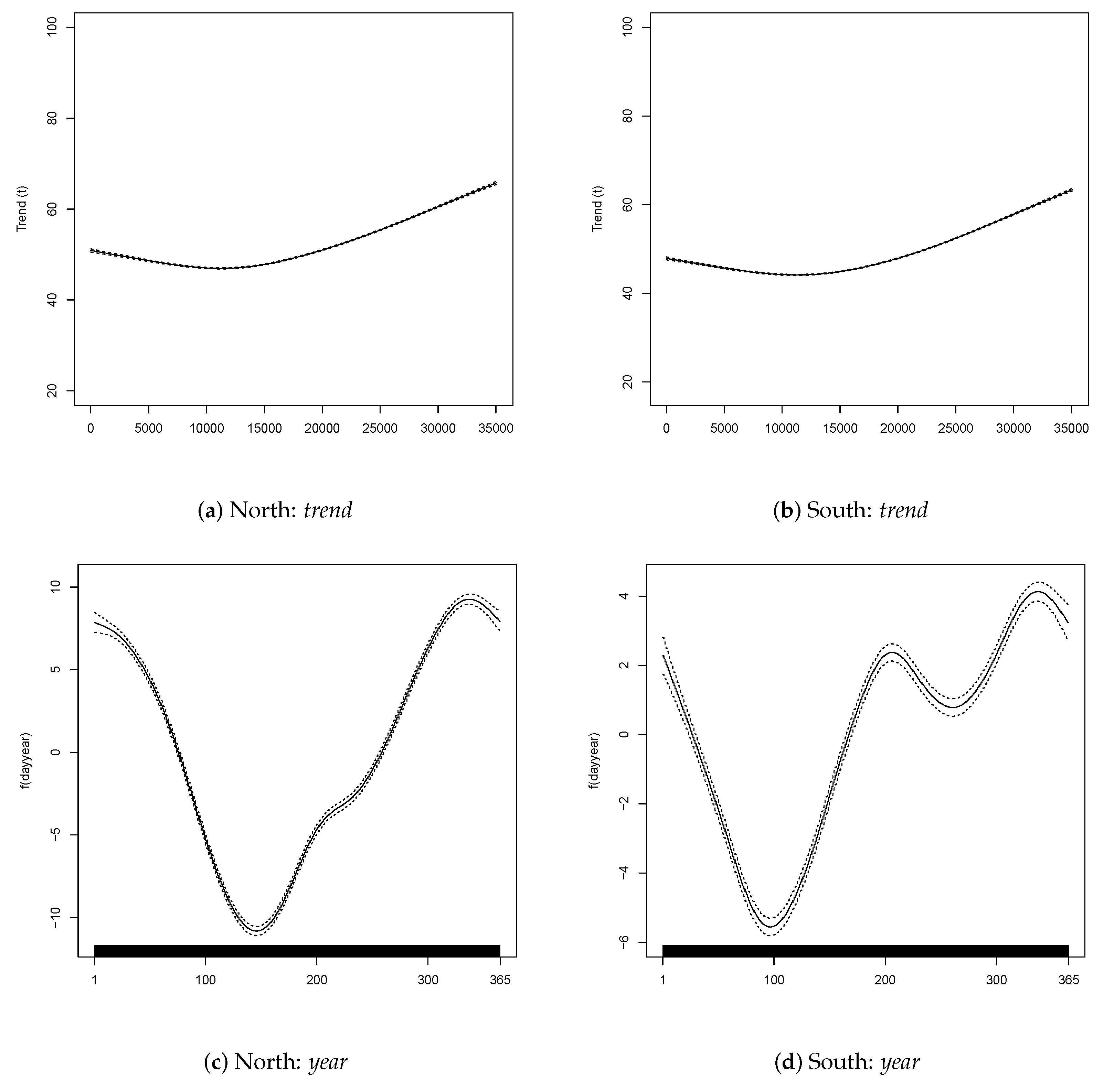
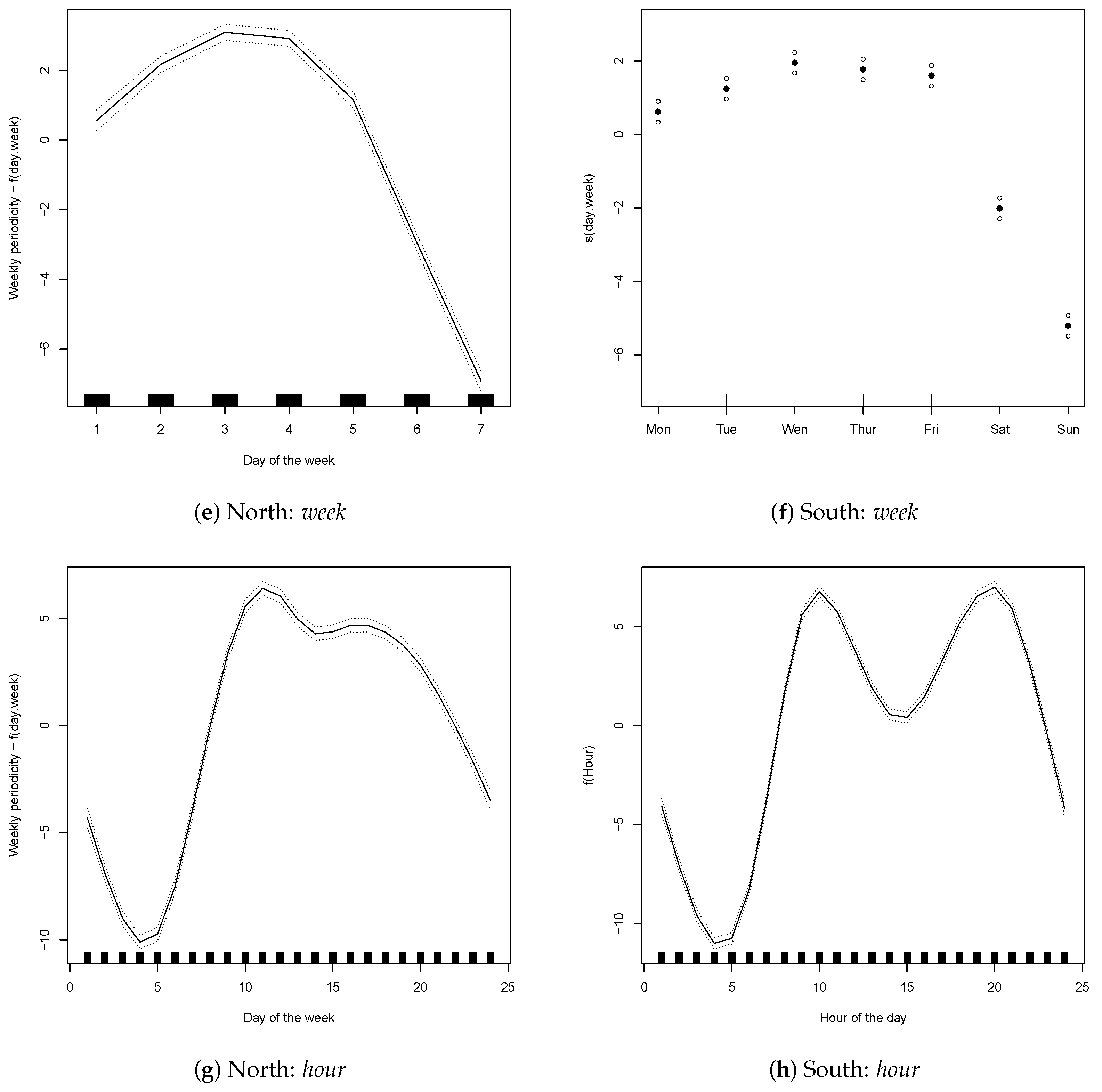
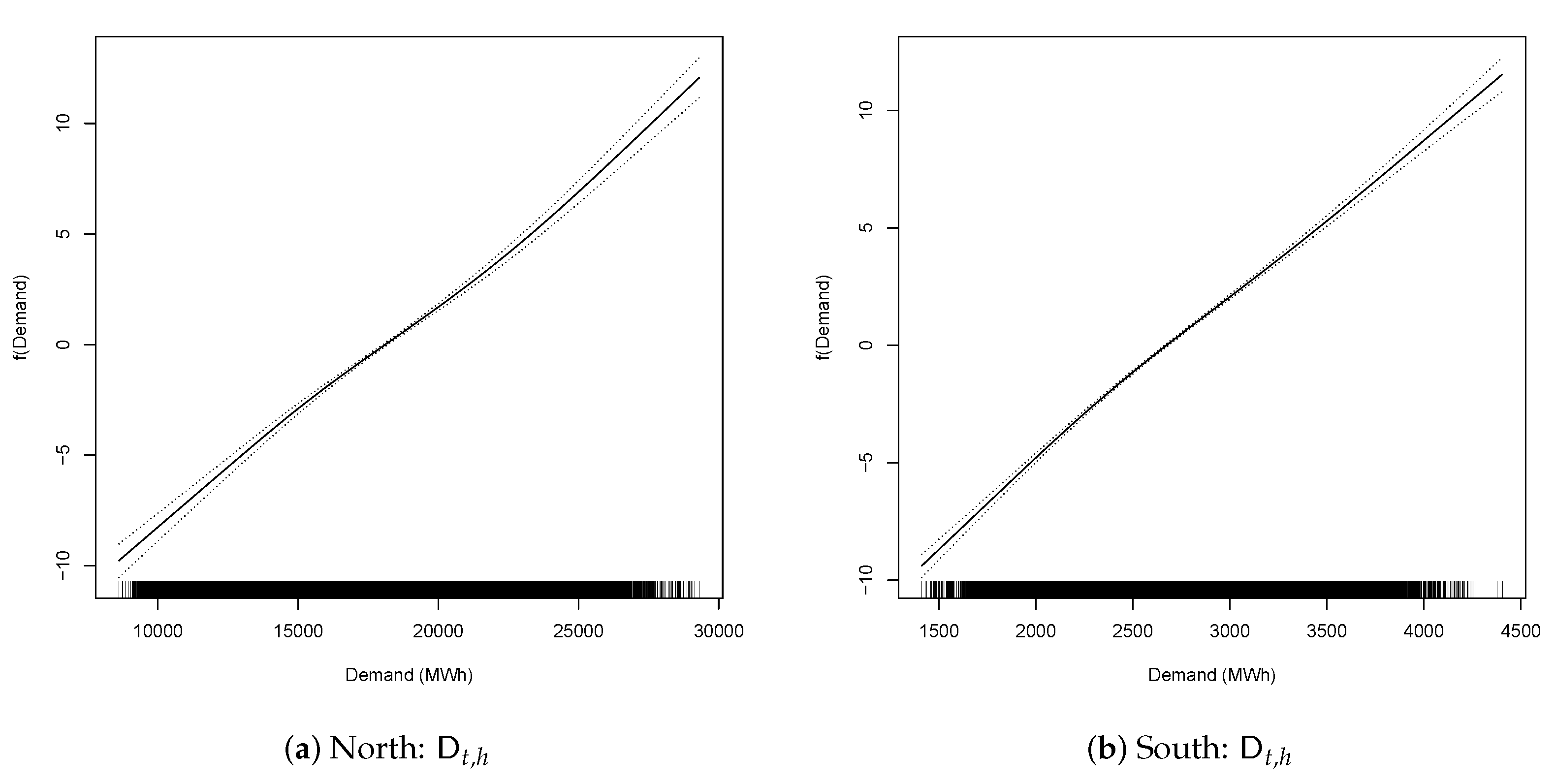
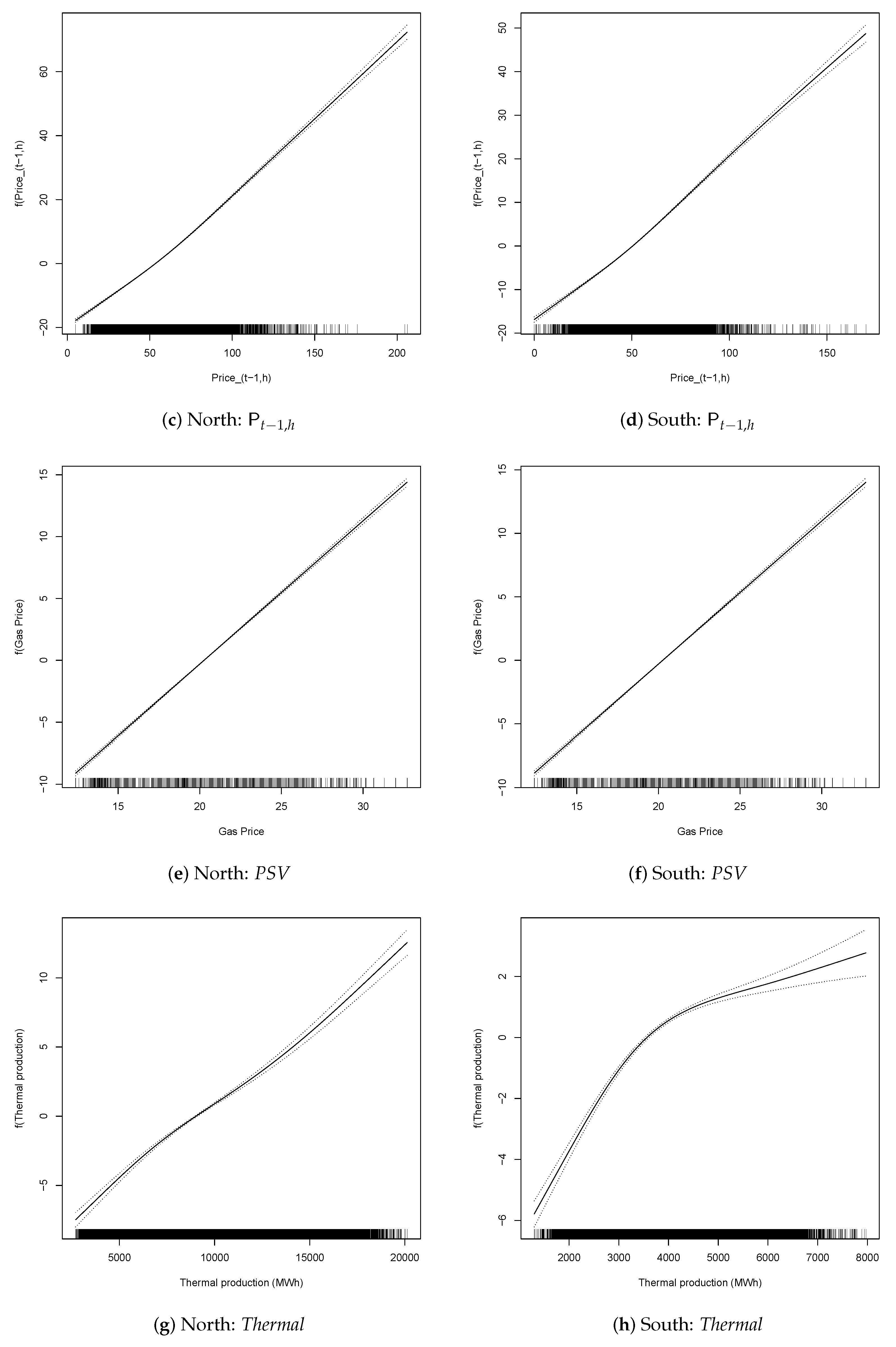
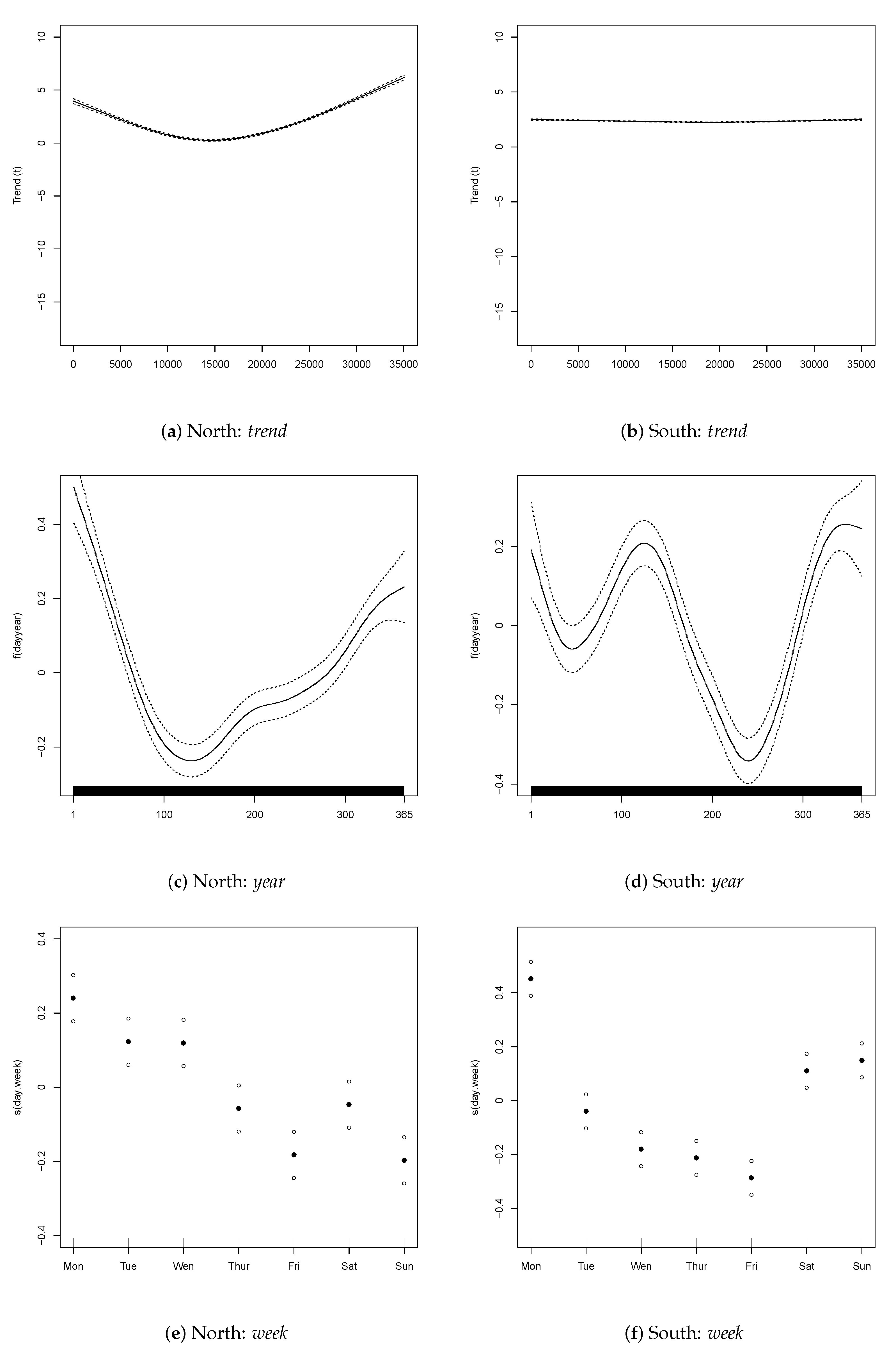
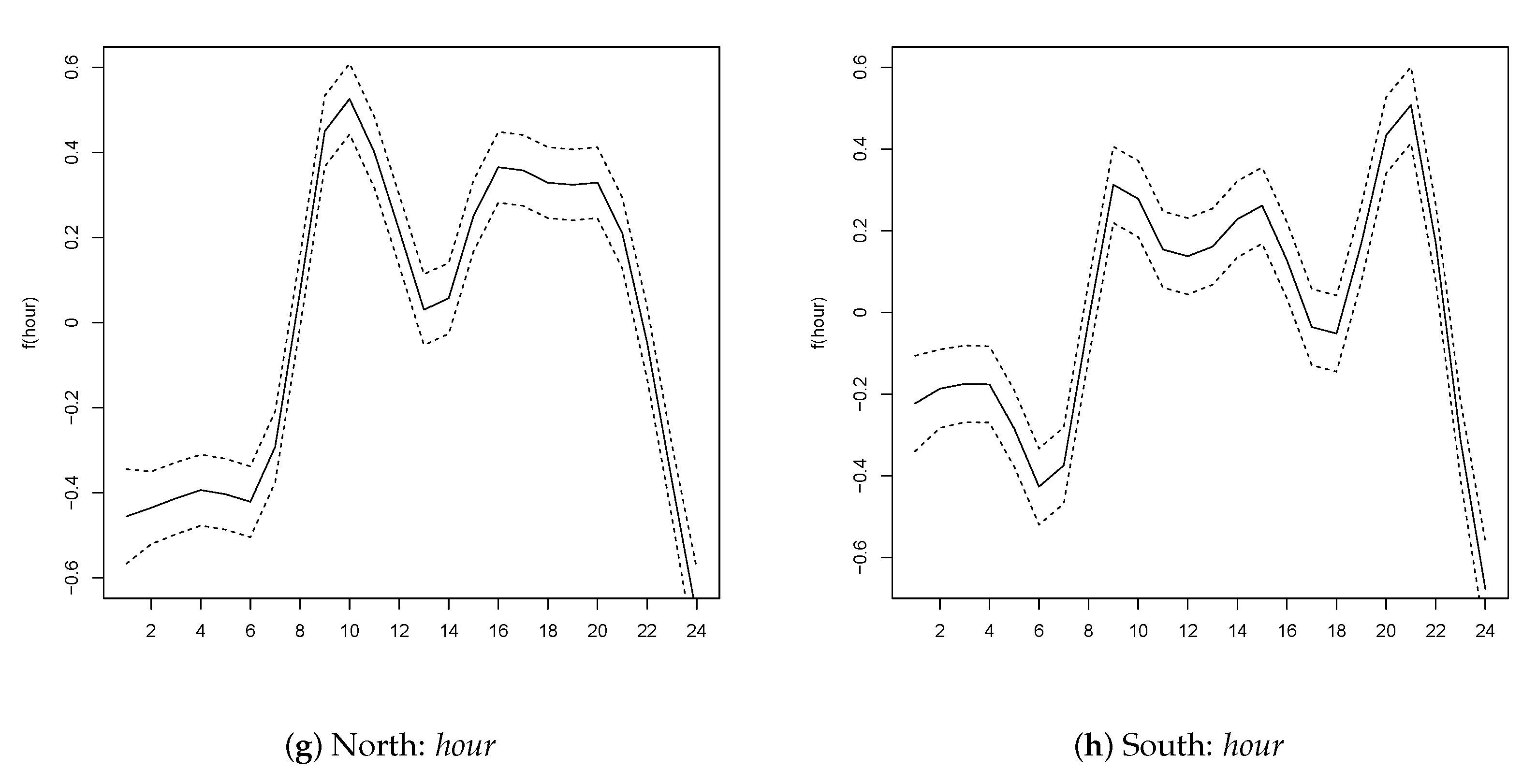
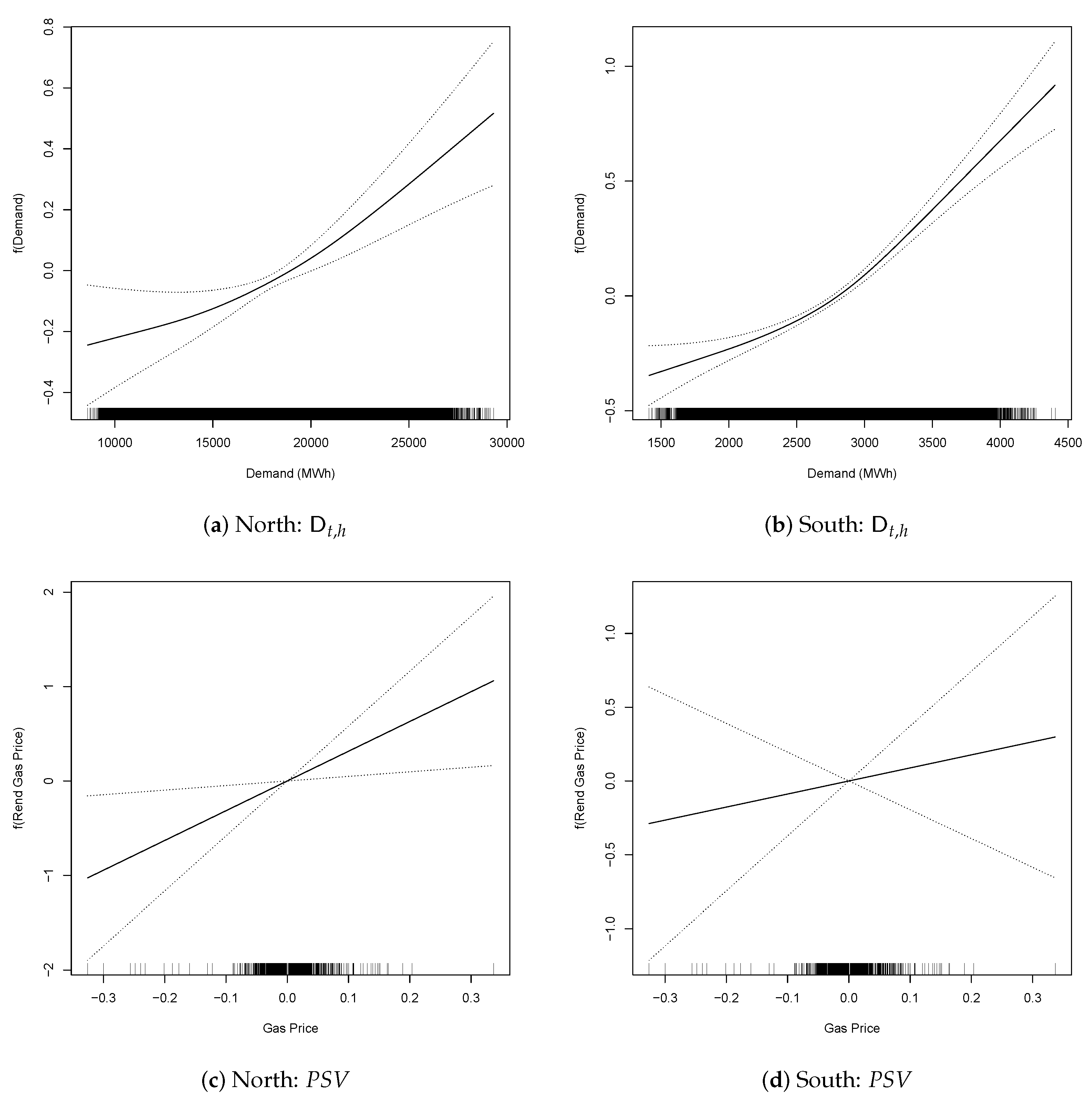
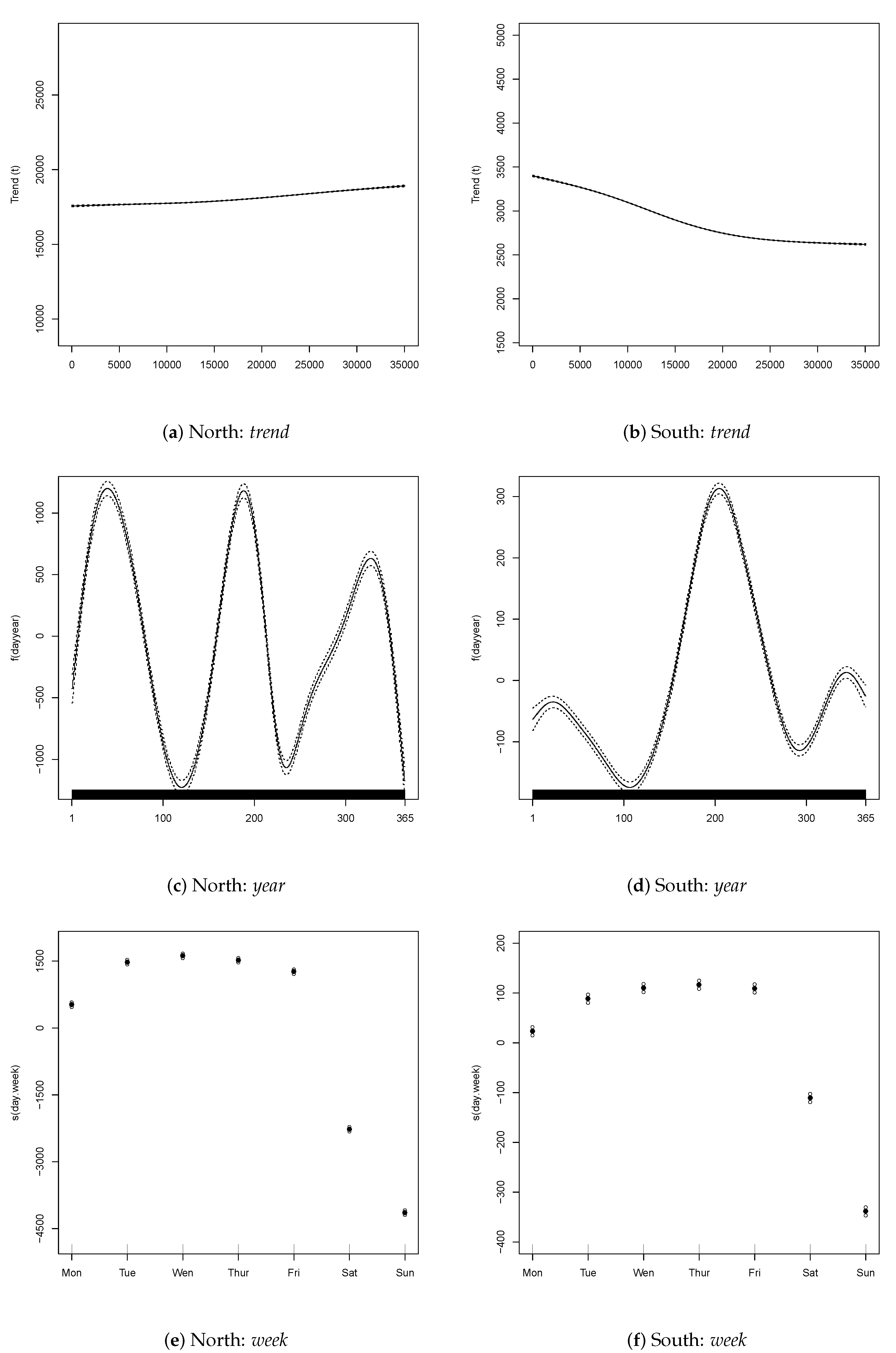
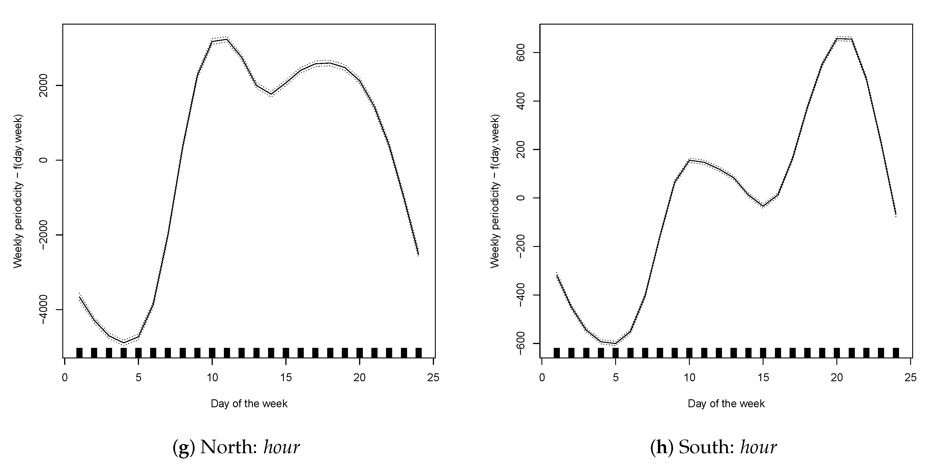
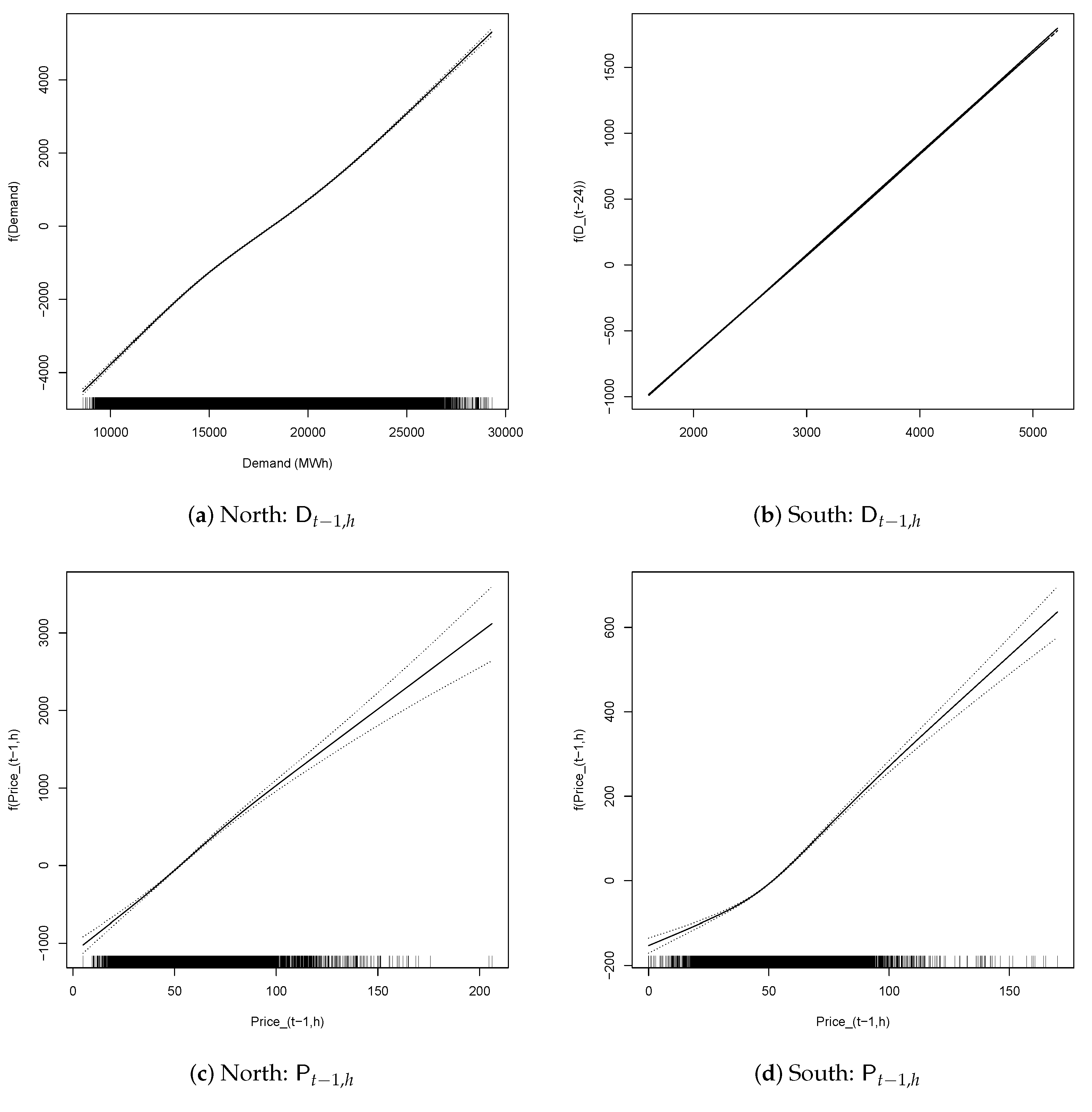
We begin by examining the effects of calendar variables: Figure 2a,b illustrate that, in both zones, a slightly parabolic trend is present which trends upwards in the second part of the series. The graphs related to the yearly periodic component (Figure 2c,d) show that prices decrease at the beginning of the year, reaching a minimum around April in the southern zone and around May–June in the northern zone and then, begin to increase again. However, while in the northern zone, they increase roughly monotonically, in the southern zone, a new local minimum around September can be observed. As expected, the shape of the weekly profile (Figure 2e,f) is very similar for the two zones, with lower prices on Saturdays and Sundays and higher levels during working days. The main difference is the differential between the maximum and minimum price which is around $5.5$ euros for the southern zone and around 9 euros for the northern zone. The effect of the different Load Periods is described in the last two panels of Figure 2. As expected, prices are higher during working hours and lower at night. They decrease up to Load Period 4 and, then, begin increasing again. However, their effect is negative through Load Period 8. After that, the effect remains positive, up to Load Periods 22–23 and, then, becomes negative again. In both zones, during the positive period, two bumps are present—mid-morning and late afternoon. In the southern zone, the two bumps are more pronounced, and the second bounce shifts by 2–3 h with respect to the northern zone. Functions describing the effects of electricity demand and lagged prices of electricity (e.g., ${\mathsf{P}}_{t-1,h}$) and gas (${\mathsf{PSV}}_{t,h}$) (Figure 3) are linear or almost linear, lagged electricity prices having a slightly greater impact in the northern zone.

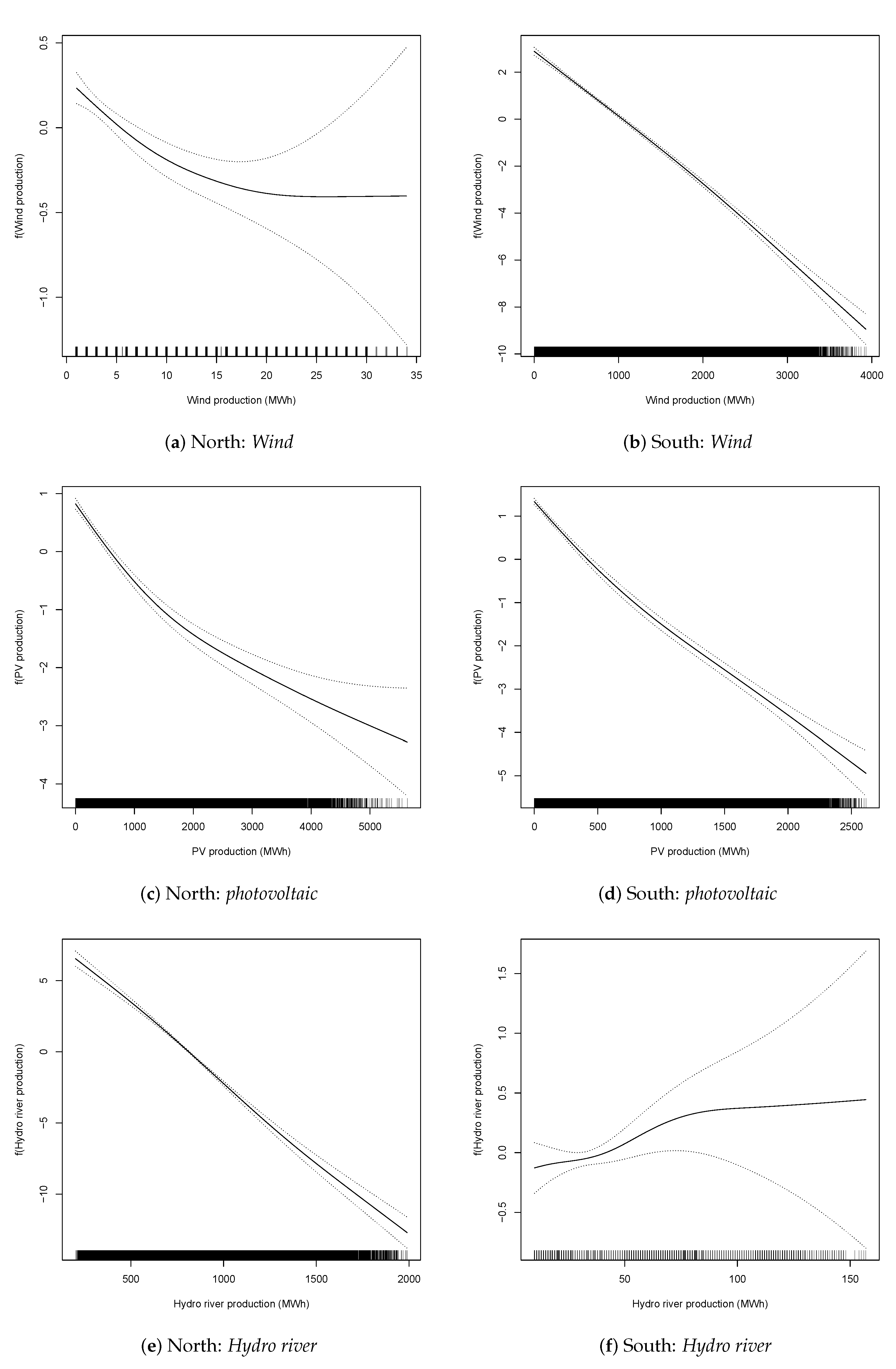
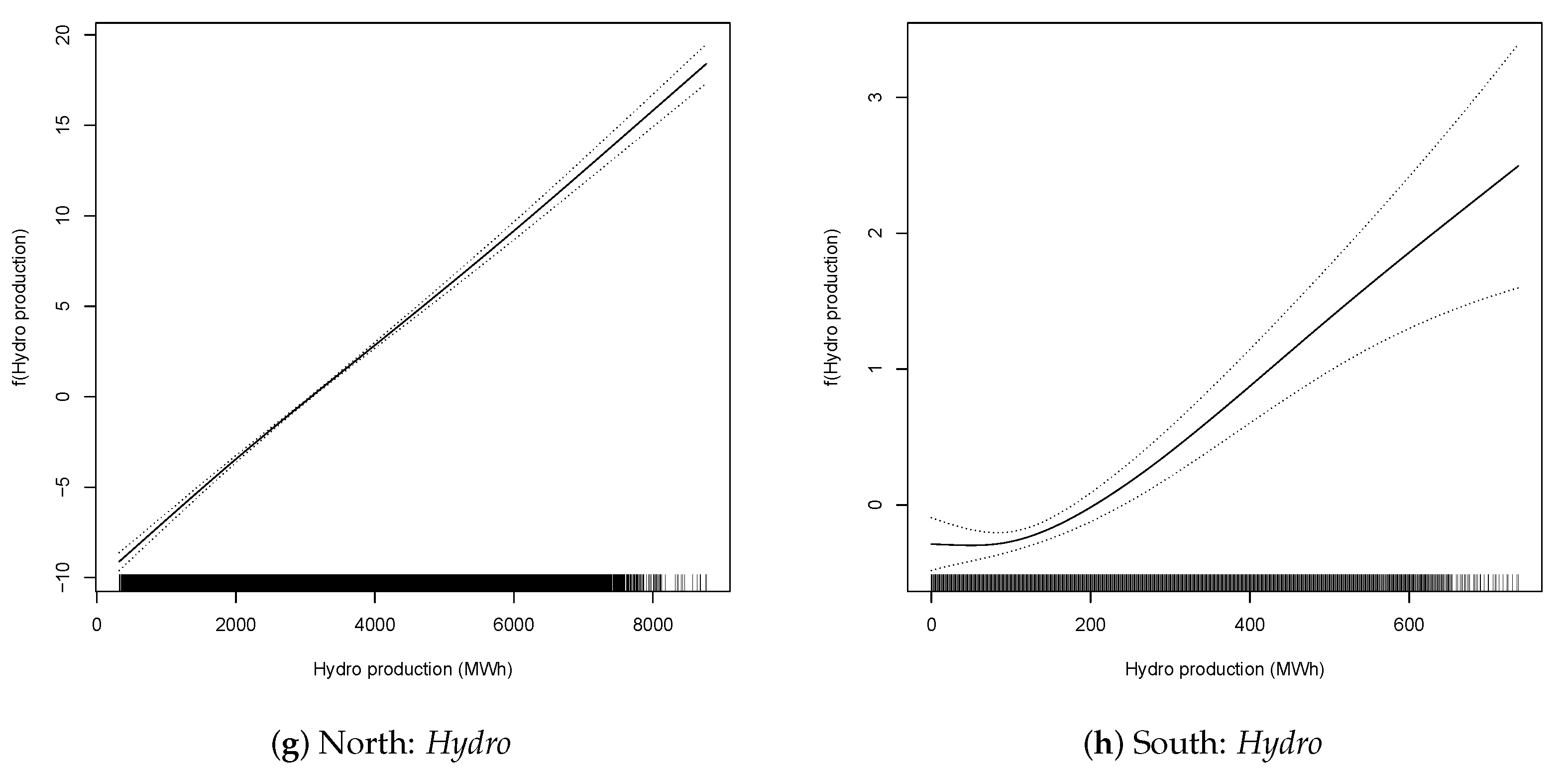
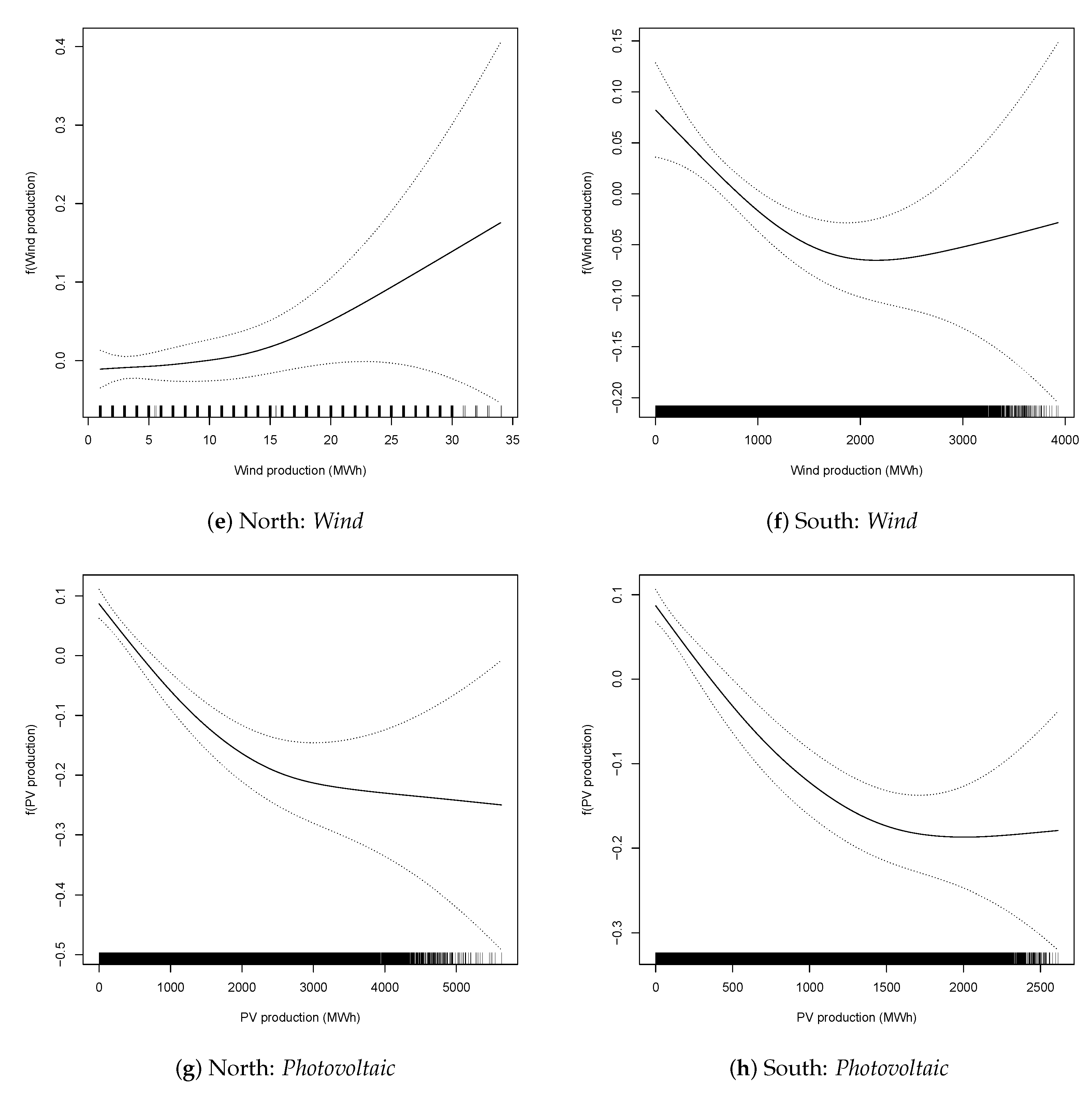
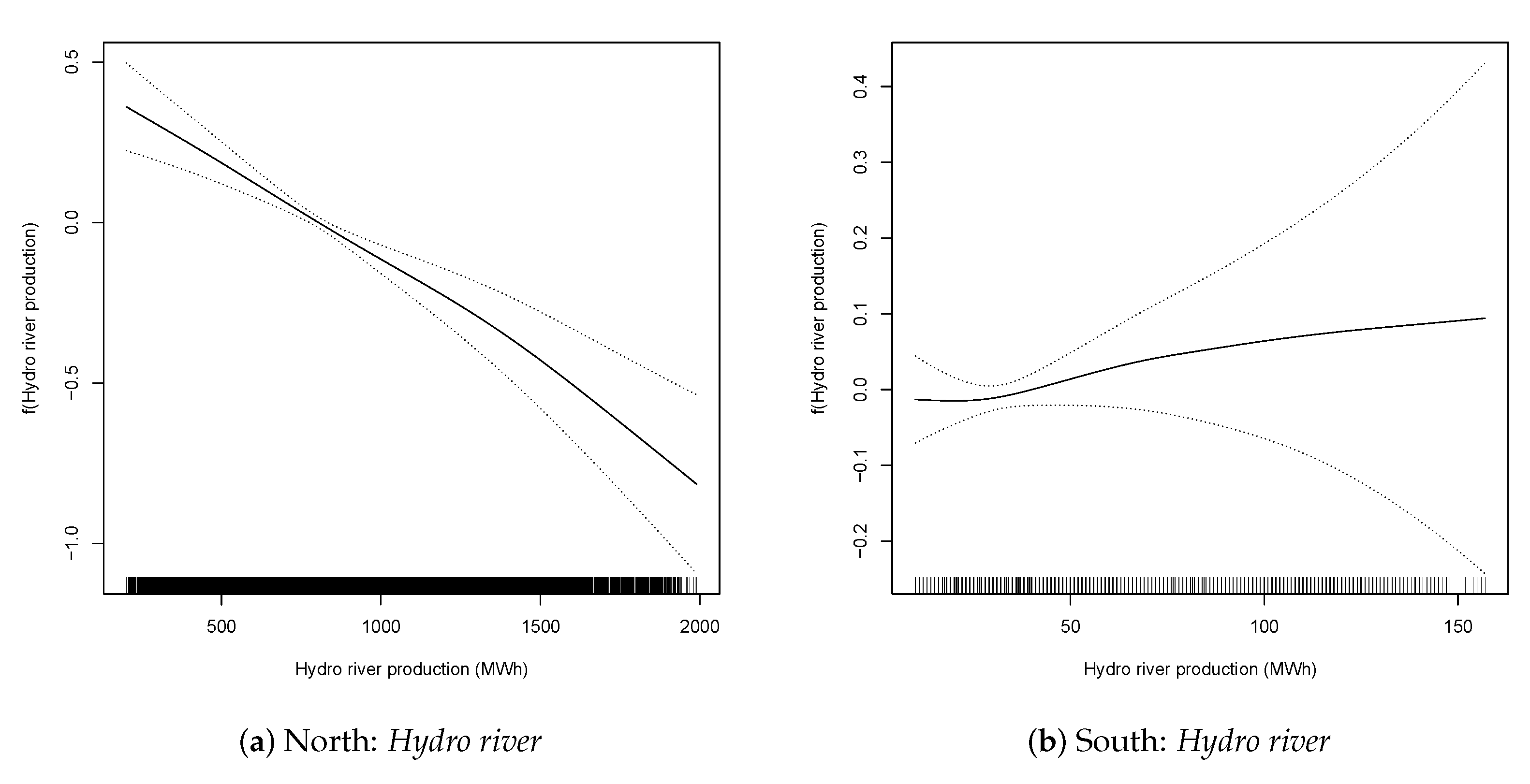
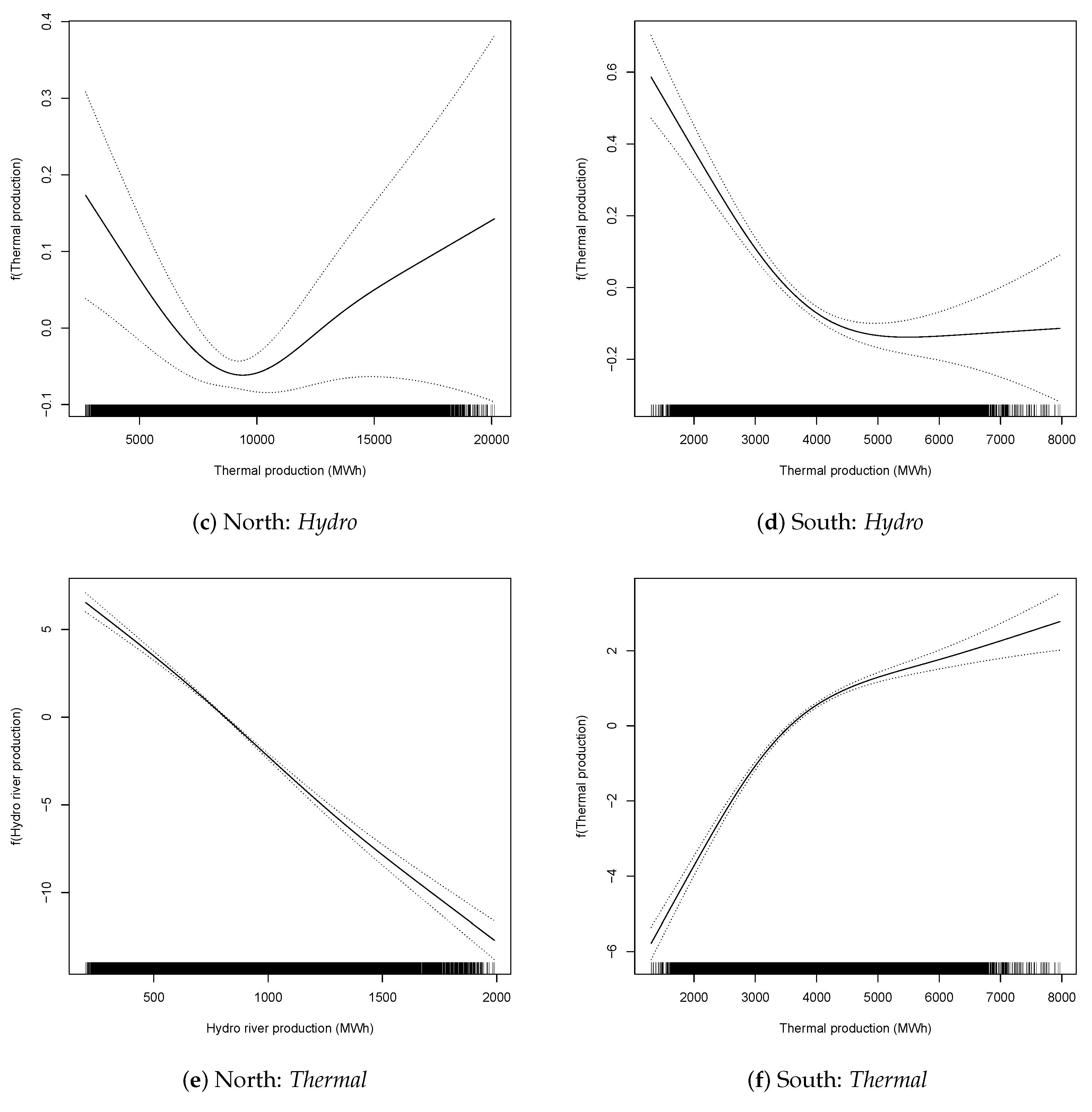
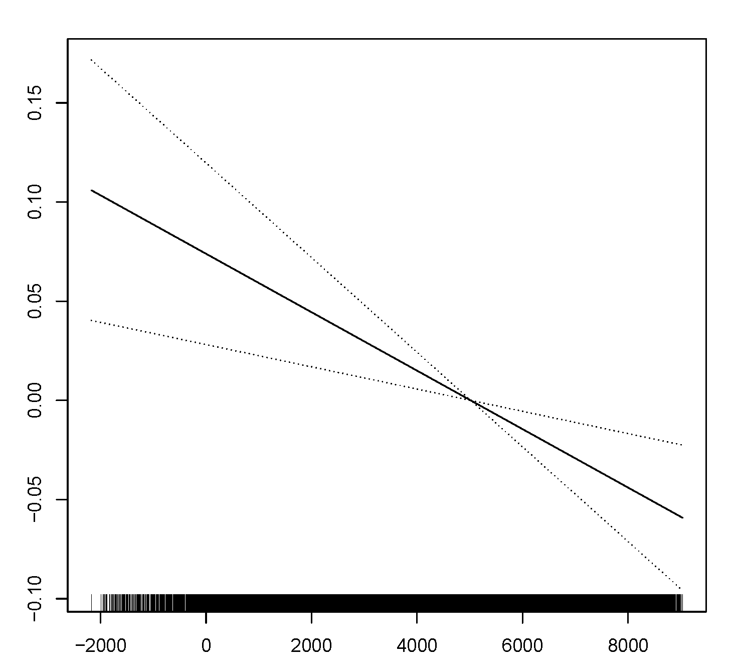
Differences between the northern and southern zones are more important when dealing with the effects of renewable energy sources (Figure 4). The data suggest a positive relationship exists between thermal energy production and prices for both zones, with a much more significant effect in the northern zone. In addition, for the southern zone the curve describing the effect of the thermal energy production tends to flatten after 5000 MWh. These results are consistent with the difference in thermal production between the zones, with the southern zone producing (in 2019) around 40% of the thermal production of the northern zone (see Table 1). Figure 4a,b show that an increment in wind energy production leads to a price decrease that is small and tends to become irrelevant in the northern zone but is clearly more significant in the southern zone. Wider intervals for large wind electricity production levels are explained by the fact that we rarely observe such high levels of wind production. Again, the huge difference in wind energy production between the two zones, reported in Table 1, explains this result. A similar inverse relationship exists also for the photovoltaic energy production (PV). In both zones, an increase in PV production leads to a decrease in the price. Even if the level of photovoltaic energy production is higher in the northern zone, in this case, the effect is slightly stronger in the southern zone. Energy production from hydro river sources in the southern zone is about $5\%$ of that in the northern zone. As a consequence, while in the northern zone an increment of this variable considerably reduces the electricity price, the same does not occur in the southern zone, where the effect is negligible (Figure 4e,f). A large difference between the two zones can also be observed with respect to hydropower from basin rivers (Figure 4g,h). In this case, however, a positive variation in hydropower production leads to an increment in the price. This is mainly due to the fact that hydro basin energy is easier to manage with respect to hydro rivers and can therefore be sold when conditions are more favourable for producers. Although this relationship is significant for both of the zones, in the southern one the impact is quite limited.

The same kind of analysis can be conducted to assess the impact of variables onto the variability (conditional variance) of prices, (see Figure 5, Figure 6 and Figure 7). In the northern zone, a parabolic trend in the evolution of price variability can be observed. As for the conditional mean, the trend is increasing in the second part of the series. On the contrary, no trend appears in the southern zone, where variability does not evolve with time. The effect of the seasons on variability is quite different in the two zones. In the north, variability shows a “V” effect, with just one minimum around April–May and a large difference between maximum and minimum variability. In the south, two minima are observed, corresponding to around February and September, but the variability range (maximum–minimum) is much less marked. In both zones, the variability is lower in the middle of the week and is higher on Mondays, Saturdays and Sundays. As expected, variability is lower at night than during the day. In the northern zone, two peaks corresponding to Load Periods 10 and 20 and a throat in Load Period 14 are observed, while in the southern zone, three less well-defined peaks occur in the graph. An increase in demand leads to an almost linear increase in variability in both zones. The relationship between variability and returns in the gas price is directly proportional but barely significant. It is interesting to analyse the effects of renewable energy productions on variability. Wind production is significant only in the southern zone, where data suggest an inverse relation between variability and wind production up to around 2000 MWh and a flattening after this level. An increase in the photovoltaic production leads in both zones to decrease variability, but only up to a certain level of production. Regarding the effect of hydro river production, the data highlight a significant inverse relationship with variability in the northern zone and an almost flat, and insignificant relationship in the southern zone. The situation is different for hydropower plants from river basins, for which the relationship is direct and significant in both zones. Finally, the relationship between thermal production and variability shows a “V” form that is barely significant in the northern zone and an inverse relationship in the southern zone.

4.2. Demand Analysis

In this section, the heteroscedastic additive model described in Section 3 is tailored to describe the dynamics of demand. As for prices, we analyse the functional form of the relationship between demand and several covariates. However, it is reasonable to assume that level of demand does not depend on the energy production source. Thus, they are not considered. Figure 8 and Figure 9 plot the estimated non-parametric functions, $f_j$, for the conditional mean, while Figure 10 and Figure 11 show functions $h_j$ included in the conditional variance.

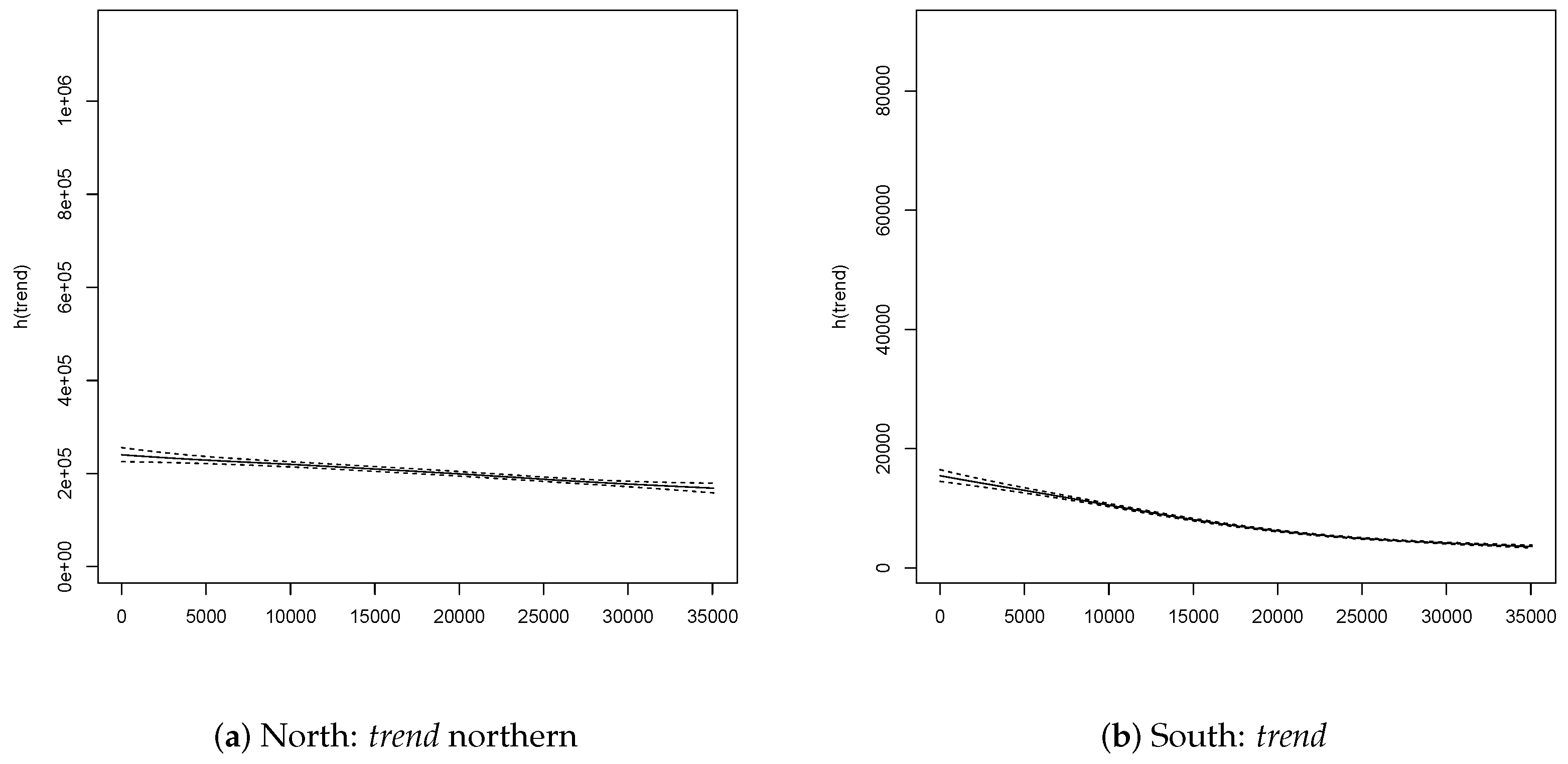
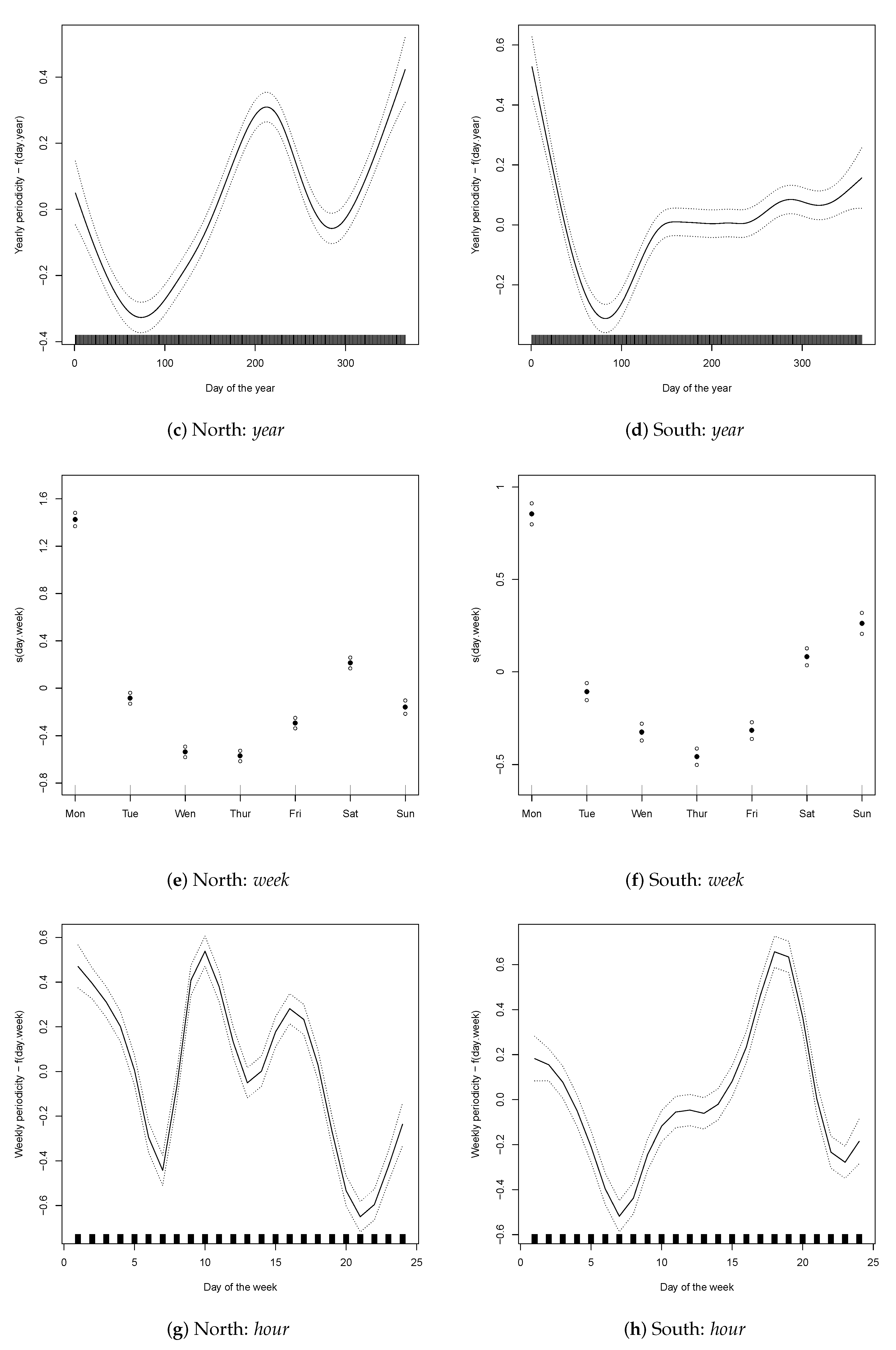
As far as the results for the calendar effects in Figure 8, it is worth noting that there are some differences between the effects of covariates between the two zones, especially concerning their magnitude. The first difference is in the trend component (Figure 8a,b), which is slightly upward in the northern zone and slightly downward in the southern zone, even if it appears to flatten in 2018. This suggest that the two zonal markets have experienced different evolutions. Completely different behaviour is observed in the two zones for yearly cycles, (see Figure 8c,d). In the northern zone, the electricity demand displays three well pronounced peaks coinciding with January–February, June and December. In the southern zone, we instead observe a major peak in about June-July, followed by a sharp contraction throughout the end of October. As expected, the weekly patterns (Figure 8e,f) are almost identical in both zones, with higher energy demand levels on Tuesdays, Wednesdays and Thursdays, with a clear decay on Fridays and during weekends. In both zones, the daily cycle (Figure 8g,h) display two major peaks: the first at around Load Period 10 and the second in late afternoon. The first peak, however, is much more important in the northern zone and demand volumes is generally much higher in the northern zone. The estimated function for the remaining covariates is plotted in Figure 9. The relationship between electricity demand ${\mathsf{D}}_{t,h}$ and its lagged value, ${\mathsf{D}}_{t-1,h}$, as well as between electricity demand and contemporary electricity price ${\mathsf{P}}_{t,h}$, are basically linear and monotonically increasing. The relationship with price seems to be counterintuitive but it can be justified by the persistence over time of demand and prices and by the documented strong correlation between demand and prices. Indeed, a high level of electricity demand tends to persist and be associated with higher prices. Therefore, there is no causal relationship between higher prices and demand levels. The same reasoning holds for the variable ${\mathsf{Import}}_{t,h}$. The upward shape of the estimated functional regression of demand on imports is due to the fact that higher demand levels are often satisfied by an increase in foreign supply. Regarding natural gas price returns (The logarithmic return is defined as $PSV.re{t}_{t,h}=log{PSV.ret}_{t,h}-log{PSV.ret}_{t,h}$) (Figure 9e,f), we observe a mild downward trend for the range of more frequent returns’ values in both zones. A possible explanation for this effect relies on the relevance of electricity production from natural gas sources in Italy. Indeed, the average electricity production from natural gas sources for 2015–2019 was about 22% of the total production worldwide and about 39% in Italy. With more than one-third of total energy production consisting of natural gas-fired generation, it is quite natural to have a downward demand curve as gas prices rise.

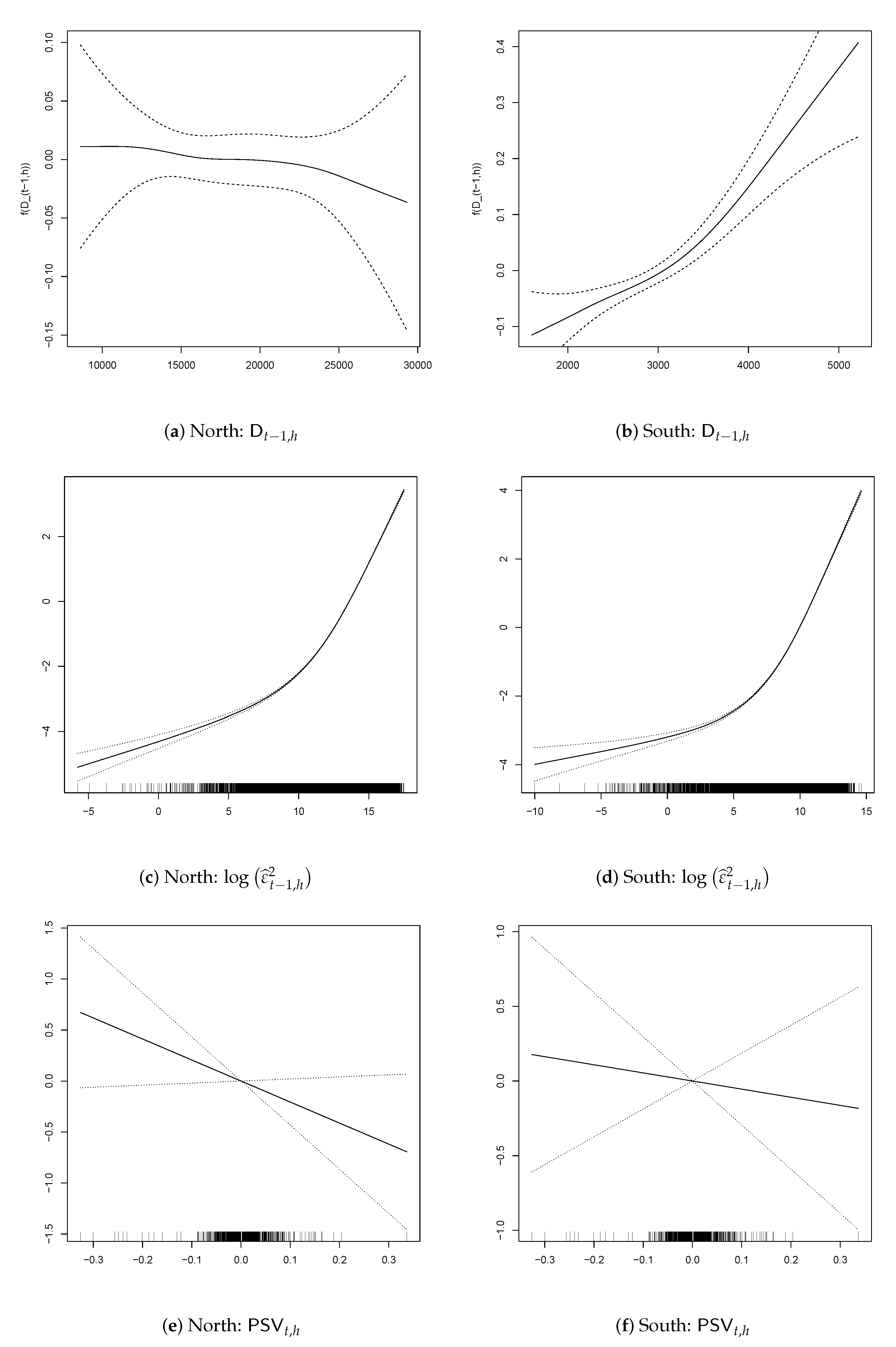
Figure 10 and Figure 11 plot the estimated functions relating the covariates and the conditional log-volatility. The estimated trend in Figure 10a,b is slightly downward for both zones over the whole period. As for the conditional mean, the structural interpretation of the overall trend is relevant for the analysis of the electricity market’s behaviour. Despite the increased electricity production from renewable sources experienced over the last few decades, the exhibited downward trend for the log-conditional volatility provides evidence of a tendency of demand uncertainty to decrease over the long–run. Visual inspection of the daily, weekly and yearly cycles in Figure 10c–h provide further important structural information about demand uncertainty. In both zones, the volatility reaches its minimum around March and, then, increases again. However, the increase in the conditional volatility during the spring and summer is much more pronounced for the northern region, perhaps due to the less predictable weather conditions and their impact on renewable energy production. In the southern zone, after a sharp decrease during the winter season, the conditional log-volatility remains at an almost constant value for the remainder of the year, suggesting substantial stability in demand volatility. The impact of the day of the week on variability for the two zones (Figure 10d,f) is similar, with higher volatility being observed on Mondays, Saturdays and Sundays. As for the conditional mean, the intra-daily cycles substantially differ for the North and South (see Figure 10c,h). In the northern zone, there are two clear peaks around Load Period 10 and around mid-afternoon, while in the southern zone, peak is observed in the late afternoon. The shape of the estimated function for the remaining covariates is plotted in Figure 11a,g. As for more traditional heteroscedastic time-series models, such as ARCH–type processes, the lagged log–squared residuals, $log\left({\widehat{\epsilon }}_{t-1,h}^2\right)$, have a strongly positive and very similar impact on demand volatility in the two zones. The effect of lagged electricity demand on current volatility (Figure 11a) is negligible, meaning that past demand does not impose a strong autoregressive effect on current conditional log-volatility. The impact of $PSV.re{t}_{t,h}$ is instead negligible in the southern zone and negative and significant in the northern zone. The downward slope of the effect of $PSV.re{t}_{t,h}$ on current northern demand volatility documents a contraction in the demand uncertainty as contemporaneous natural gas log-returns increases. Finally, the importation of energy in Figure 11g negatively impacts current demand volatility, but only for high positive values.

5. Out-of-Sample Forecasting

In this section we examine the forecasting performance of the previous models, both in terms of point prediction and interval prediction, which is also known as probabilistic prediction in the energy literature. To this end, data referring to the period between 1 January 2015 and 31 December 2018 are used to identify and estimate the models, while data referring to the entire year of 2019 are used for out-of-sample evaluation of forecasts.

The semi-parametric heteroscedastic additive models used are, basically, those defined in Section 3. In this case, however, we separately model and forecast the daily time series of each load period of the day. This leads to 24, possibly different, models, increases the flexibility and enable the omission of the hour-of-the-day variables. The one-day-ahead forecasts of each load period are then combined to obtain the hourly time series of one-day-ahead forecasts for the entire year of 2019. Moreover, since we use models for out-of-sample forecasting, except for calendar variables, only lagged variables enter the models. Another alternative, not pursued here, would have been to consider suitable forecasts of covariates.

To select the significant (lagged) variables and identify the predictive models, an in-sample analysis based on a stepwise procedure and data from 2015 to 2018, was performed for each of the 24 daily time series and for each zone, both for the conditional mean and the conditional variance.

Table 2. Selected variables for the predictive models for the conditional mean of price in the northern and southern zones.

Variables	Norhtern Zone—Load Periods						Southern Zone—Load Periods
	1–6	7–11	12	13–20	21	22–24	1–3	4–6	7–9	10–20	21–24
${\mathsf{trend}}_{t,h}$	√	√	√	√	√	√	√	√	√	√	√
$\mathsf{day}.{\mathsf{year}}_{t,h}$	√	√	√	√	√	√	√	√	√	√	√
$\mathsf{day}.{\mathsf{week}}_{t,h}$	√	√	√	√	√	√	√	√	√	√	√
${\mathsf{bank}}_{t,h}$	√	√	√	√	√	√	-	-	√	√	-
${\mathsf{P}}_{t-1,h}$	√	√	√	√	√	√	√	√	√	√	√
${\mathsf{D}}_{t-1,h}$	√	√	√	√	√	√	√	√	√	√	√
${\mathsf{Wind}}_{t-1,h}$	-	-	√	-	-	-	√	√	√	√	√
${\mathsf{PV}}_{t-1,h}$	-	√	√	√	-	-	-	-	√	√	-
${\mathsf{Hydro}}_{t-1,h}$	√	√	√	-	-	√	-	-	-	√	√
$\mathsf{Hydro}.{\mathsf{R}}_{t-1,h}$	√	√	√	√	√	√	-	-	-	√	√
${\mathsf{Therm}}_{t-1,h}$	√	√	√	√	√	√	√	-	-	√	√
${\mathsf{Import}}_{t-1,h}$	√	√	√	√	√	√	-	-	-	-	-
${\mathsf{PSV}}_{t-1,h}$	√	√	√	√	√	√	√	√	√	√	√

,

Table 3. Selected variables for the predictive models for the conditional variance of price in the northern zone.

Variables	Norhtern Zone—Load Periods
	1–3	4–6	7–8	9–10	11–13	14–16	17–19	20–22	23–24
${\mathsf{trend}}_{t,h}$	-	-	-	-	-	-	-	-	-
$\mathsf{day}.{\mathsf{year}}_{t,h}$	√	√	√	√	√	√	√	√	√
$\mathsf{day}.{\mathsf{week}}_{t,h}$	-	√	√	√	√	√	√	√	√
${\mathsf{bank}}_{t,h}$	-	-	-	-	-	-	-	-	-
$log\left({\epsilon }_{t-1,h}^2\right)$	√	√	√	√	√	√	√	√	√
${\mathsf{D}}_{t-1,h}$	-	-	-	√	√	√	√	√	√
${\mathsf{Wind}}_{t-1,h}$	-	-	-	√	√	√	-	-	-
${\mathsf{PV}}_{t-1,h}$	-	-	√	√	√	√	√	-	-
${\mathsf{Hydro}}_{t-1,h}$	√	√	√	√	-	-	√	√	√
$\mathsf{Hydro}.{\mathsf{R}}_{t-1,h}$	√	√	√	√	-	√	-	-	√
${\mathsf{Therm}}_{t-1,h}$	√	√	√	√	√	√	√	√	√
${\mathsf{Import}}_{t-1,h}$	-	-	-	-	-	-	-	-	-
$\mathsf{PSV}.{\mathsf{ret}}_{t-1,h}^2$	√	√	√	-	√	√	√	-	-

,

Table 4. Selected variables for the predictive models for the conditional variance of price in the southern zone.

Variables	Southern Zone—Load Periods
	1–3	4–10	11–13	14–15	16–17	18–22	23–24
${\mathsf{trend}}_{t,h}$	-	-	-	-	-	-	-
$\mathsf{day}.{\mathsf{year}}_{t,h}$	√	√	√	√	√	√	√
$\mathsf{day}.{\mathsf{week}}_{t,h}$	-	√	-	√	-	√	-
${\mathsf{bank}}_{t,h}$	-	-	-	-	-	-	-
$log\left({\epsilon }_{t-1,h}^2\right)$	√	√	√	√	√	√	√
${\mathsf{D}}_{t-1,h}$	√	√	√	√	√	√	√
${\mathsf{Wind}}_{t-1,h}$	-	√	√	√	√	√	-
${\mathsf{PV}}_{t-1,h}$	-	-	√	√	√	√	√
${\mathsf{Hydro}}_{t-1,h}$	-	-	-	-	-	-	-
$\mathsf{Hydro}.{\mathsf{R}}_{t-1,h}$	-	-	-	-	-	-	-
${\mathsf{Therm}}_{t-1,h}$	-	-	√	√	√	√	√
$\mathsf{PSV}.{\mathsf{ret}}_{t-1,h}^2$	√	√	√	-	√	√	√

and

Table 5. Variables included in the predictive models for the conditional mean and conditional variance of demand.

Variables	Norhtern Zone—Load Periods		Southern Zone—Load Periods
	Condi. Mean	Cond. Variance	Condi. Mean	Cond. Variance
${\mathsf{trend}}_t$	√	√	√	√
$\mathsf{day}.{\mathsf{year}}_t$	√	√	√	√
$\mathsf{day}.{\mathsf{week}}_t$	√	√	√	√
${\mathsf{bank}}_t$	√	√	√	√
$logre{s}_{t-1,h}^1$	-	√	-	√
${\mathsf{D}}_{t-1,h}$	√	√	√	√
${\mathsf{D}}_{t-7,h}$	√	√	√	√
$\mathsf{Import}.{\mathsf{R}}_{t-1,h}$	√	√	-	-
$\mathsf{PSV}.{\mathsf{ret}}_{t-1,h}$	√	-	√	-
$\mathsf{PSV}.{\mathsf{ret}}_{t-1,h}^2$	-	√	-	√

provide a complete list of the specific variables used for out-of-sample prediction in each load period.

At a daily frequency, the residual autocorrelation of these models changes with the hour of the day but is, generally, very weak. In addition, when it is a bit stronger, it is hardly exploitable for prediction. The residual ACF could be easily whitened by considering the variant of the model described in [63]. Since we focus on prediction, we do not pursue this approach. The residual intra-daily autocorrelation is still clearly present because it has not been modelled.

The results are summarized in Table 2, Table 3 and Table 4 for prices and in Table 5 for demand. Please note that for demand, we did not consider renewable energy productions. Five models were considered: all of them have the same specification for the conditional mean but differ for their specifications of conditional variance. For the latter, we considered a homoscedastic model, a Gaussian GARCH $(1,1)$ model, a Student-t GARCH $(1,1)$ model, a Full–GAM model and a Calendar–GAM, i.e., a GAM model with only calendar explicative variables.

Furthermore, for the Full–GAM model and a Calendar–GAM, the non–parametric prediction intervals are obtained according to expression (6), where quantile $q_z\left(\alpha \right)$ is the empirical quantile of the in-sample standardised residuals ${\widehat{z}}_t=(y_t-{\widehat{\mu }}_t)/{\widehat{\sigma }}_t$.

Point forecasts and related models were evaluated in terms of Mean Absolute predictive Error (MAE) and Mean Absolute Percentage predictive Error (MAPE). Interval forecasting was evaluated, at the $80\%$, $90\%$ and $95\%$ confidence levels, in terms of the deviation of the observed coverage (OC) from the nominal coverage (NC) as well as in terms of the forecasting intervals’ mean (MW).

5.1. Price Forecasting: Results

Table 2 lists, for each load period, the (significant) variables are included in the models for the conditional mean prediction for the northern and southern zones. In both zones, the models can be clustered according to the hour of the day. In the northern zone models have three different specifications corresponding to night (Load Periods 1–6 and 22–24), morning (Load Periods 7–11) and afternoon (Load Periods 13–20). Load periods 12 and 21 required individual specifications. In addition in the southern zone there are five different models corresponding to Load Periods 1–3, Load Periods 4–6, Load Periods 7–9, Load Periods 10–20 and Load Periods 21–24.

Calendar variables are always significant, except for the bank holidays dummy variables in some Load Periods in the southern zone. Lagged price, demand, imports (only for the northern zone) and PSV price are included in the model for all Load Periods. Most of the other variables are significant but, as expected, the photovoltaic production is not during the night hours. Moreover, wind production is barely significant in the northern zone, while is always highly significant in the southern zone. Variables Hydro and Hydro.river, although significant from 10 a.m. to 12 p.m. in the southern zone, are less relevant in the northern zone. Thermal production is always included in the models for the northern zone and in most hours for the southern zone.

Likewise, Table 3 and Table 4 list the selected variables for the conditional variance models. In this case, the log-squared residual of the conditional mean, $log{\widehat{\epsilon }}_{t-1,h}^2$ was also considered. For the conditional variance, the clusters of models are much more fragmented. Variables ${\mathsf{Trend}}_t$, ${\mathsf{Bank}}_t$ and ${\mathsf{Import}}_{t-1,h}$ were never significant. On the contrary ${\mathsf{dayyear}}_t$, ${\mathsf{dayweek}}_t$, $log{\widehat{\epsilon }}_{t-1,h}^2$ and ${\mathsf{Therm}}_{t-1,h}$ were significant for all Load Periods.

The predictive results for prices are summarised—for the whole out-of-sample period 2019—in

Table 6. Electricity prices for the northern zone. Out-of-sample predictive results for the year 2019. For all models the MAE is equal to $4.36$ and the MAPE is equal to $10.1\%$. Moreover, “observed cov.” stands for nominal coverage, and “ av. width” is the mean interval forecasting width at the $(1-\alpha )$ level.

Nominal Coverage	80%		90%		95%
	Observed Cov.	Av. Width	Observed Cov.	Av. Width	Observed Cov.	Av. Width
homoscedastic	77.6	13.1	90.8	18.9	96.6	25.8
GARCH $(1,1)$–N	83.3	15.1	91.5	19.4	95.5	23.1
GARCH $(1,1)$–t	88.1	17.3	95.7	23.7	98.3	30.4
Calendar–GAM	77.7	13.3	89.6	18.3	95.5	24.0
Full–GAM	77.8	13.6	89.7	18.6	95.1	23.8

for the northern zone, and in

Table 7. Electricity prices for the southern zone. Out-of-sample predictive results for the year 2019. For all models the MAE is equal to $6.40$ and the MAPE is equal to $22.4\%$, while it is equal to $11.5\%$ if we condition to prices greater than their third empirical percentile. Moreover, “observed cov.” stands for nominal coverage, and “av. width” is the mean interval forecasting width at the $(1-\alpha )$ level.

Nominal Coverage	80%		90%		95%
	Observed Cov.	Av. Width	Observed Cov.	Av. Width	Observed Cov.	Av. Width
homoscedastic	71.10	15.40	84.60	22.70	92.00	31.70
GARCH(1,1)–N	81.80	20.90	89.20	26.80	93.40	31.90
GARCH(1,1)–t	87.80	25.50	94.90	35.60	97.90	46.50
Calendar–GAM	71.40	16.40	83.30	22.90	91.00	30.30
Full–GAM	75.4	18.50	87.20	25.20	92.89	33.30

for the southern zone.

Predictive results for the demand forecasting are summarised—for the entire year of 2019—in

Table 8. Electricity demand for the northern zone. Out-of-sample predictive results for the year of 2019. For all of the models the MAE is equal to $500.8$ MWh and MAPE is equal to $2.8\%$. Moreover, “observed cov.” stands for nominal coverage, and “av. width” is the mean interval forecasting width at the $(1-\alpha )$ level.

Nominal Coverage	80%		90%		95%
	Observed Cov.	Av. Width	Observed Cov.	Av. Width	Observed Cov.	Av. Width
homoscedastic	81.8	1510.1	90.9	2250.4	95.3	3222.9
GARCH $(1,1)$–N	87.9	1894.7	93.8	2431.8	96.1	2897.6
GARCH $(1,1)$–t	92.8	2293.5	97.0	3214.7	98.3	4225.5
Calendar–GAM	82.1	1525.1	90.8	2081.7	95.6	2750.8
Full–GAM	80.2	1527.3	89.2	2033.9	94.2	2533.4

for the northern zone and in

Table 9. Electricity demand for the southern zone. Out-of-sample predictive results for the year of 2019. For all of the models the MAE is equal to $65.25$ MWh and MAPE is equal to $2.4\%$. Moreover, “observed cov.” stands for nominal coverage, and “av. width” is the mean interval forecasting width at the $(1-\alpha )$ level.

Nominal Coverage	80%		90%		95%
	Observed Cov.	Av. Width	Observed Cov.	Av. Width	Observed Cov.	Av. Width
homoscedastic	90.5	291.5	97.4	440.3	99.0	601.3
GARCH$(1,1)$–N	86.0	241.5	91.9	309.9	95.1	369.3
GARCH $(1,1)$–t	89.7	278.9	95.4	382.5	98.0	490.5
Calendar–GAM	88.6	268.1	96.5	393.1	98.7	525.5
Full–GAM	85.1	235.8	93.4	325.7	97.0	421.3

for the southern zone.

Regarding the price’s point prediction of the conditional mean, the mean absolute errors over the whole 2019 period were $MAE=4.36$ euros for the northern zone and $MAE=6.40$ euros for the southern zone. The corresponding percentage errors were $MAPE=10.1\%$ (North) and $MAPE=22.4\%$ (South). The MAPE for the southern zone is quite large, but that is mainly due to errors related to very small prices. Indeed, if we exclude prices smaller than their $3\%$ quantile, the MAPE has halved.

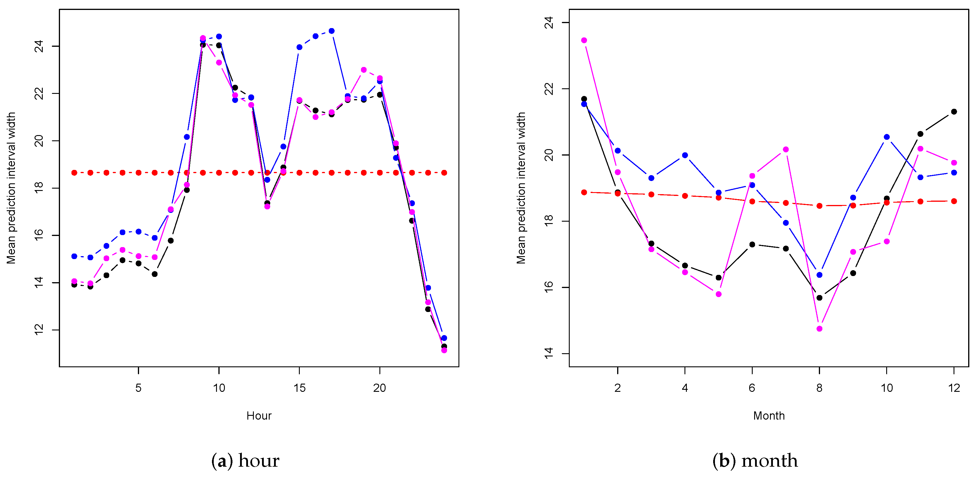
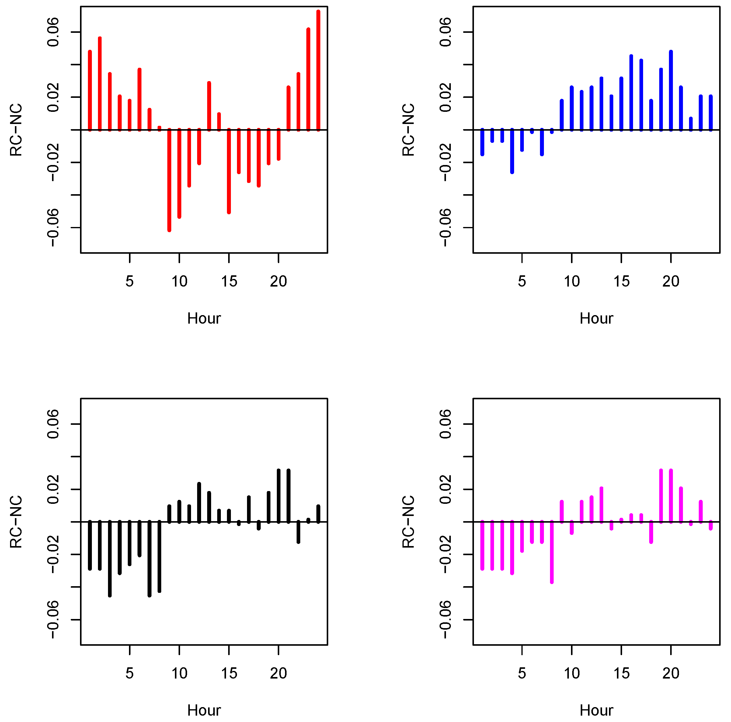
For interval forecasting, we have five models for each zone. For the northern zone, apart from the GARCH $(1,1)$–t, whose observed coverage is systematically larger than the nominal one, all remaining models seem to provide satisfactory results. However, Figure 12a,b showing the hourly and monthly mean interval prediction widths (nominal coverage 90%), points out that the homoscedastic model is unable to describe both the daily and seasonal dynamic variability, represented by the mean interval forecasting width. In addition, Figure 13, showing the differences between the hourly observed and nominal coverage, points out that the homoscedastic model provides the poorest results and suggests that its apparently good performance is the consequence of a compensation effect among hourly coverages. For brevity, the hourly and monthly mean interval forecasting widths are shown only for the northern zone’s price, but a similar behaviour occurs also for demand and for the southern zone. Among the remaining models, both the Full–GAM and the GARCH $(1,1)$–N model provide satisfactory results in terms of coverage and are competitive between them. Nevertheless, on average, the Full–GAM model leads to narrower prediction intervals and is, therefore preferable. Similar considerations can be made for the southern zone but, in this case, the situation reverses, with the GARCH$(1,1)$–N model giving the best results.

5.2. Demand Forecasting: Results

For demand forecasting, we moved in the same way as for prices. The model specification is simpler because it is known that energy demand is inelastic to production from renewable sources. Thus, in our forecasting demand exercise, we do not include them in the set of possible regressors, which include calendar variables, lagged demand, (lagged) imports, prices and PSV returns. Moreover, for demand, the specification was the same for all Load Periods for both the northern and southern zones. Table 5 lists, for both zones, the variables included in the model for the conditional mean and variance specification.

Regarding the price’s point prediction of the conditional mean, the mean absolute errors for the two zones are quite similar: $MAE=500.8$ MWh for the northern zone, corresponding to $MAPE=2.8\%$, for the northern zone and $MAE=65.25$, corresponding to the $MAPE=2.4\%$ for the southern zone. When considering the interval forecasting, the results are qualitatively similar to those for prices. In the northern zone, the best results are clearly obtained using the Full GAM model, which leads to very good coverages and to the smallest mean width of the forecasting intervals. The second best models are the homoscedastic model, with the limits already described for prices, and the Calendar GAM model. The GARCH $(1,1)$-N model is in the fourth position.

When we examine the southern zone, all of the models show observed coverages larger than the nominal ones. Globally, however, the two models giving the best results are, again, the Full-GAM and the GARCH $(1,1)$-N, with the former working better for NC = 80% and the latter for NC = 90% and NC = 95%.

6. Conclusions and Discussion

In this study, a semi-parametric additive heteroscedastic regression model was proposed and applied to time series of zonal prices and demand data for the Italian electricity market to obtain point and interval forecasts. The main novelty of this approach consists of modelling both the conditional mean and the conditional variance as non-parametric functions of several covariates. Covariates describes the long-term dynamic of the series, several different kinds of periodicity as well as the impact of renewable energy sources and other market variables. The structural interpretability of the output of the model is one of the distinguishing features of our proposal. For prices, in particular, this enables us to examine the impact of renewable energy sources on the variability of prices.

Focusing on interval prediction, rather than on point prediction, allows us to understand how the available covariates impact the overall variability of price and demand and their variance and provides important probabilistic information to market operators for making decisions.

Out-of-sample predictions of zonal prices and demand were performed for the whole year of 2019 for the northern and southern zones of the Italian electricity markets. The performance of point predictions was assessed in term of mean absolute (percentage) prediction error. Forecasting intervals, instead, were evaluated with respect to coverage (e.g., observed versus nominal coverage) and average interval’ width.

While point predictions were always produced using the same semi-parametric model, forecasting intervals were obtained by using different models for the conditional variance. We considered a homoscedastic semi-parametric model, two GARCH models with Gaussian (GARCH-N) and Student-t (GARCH-T) innovation, the Calendar-GAM model, including only calendar variables, and the Full-GAM specification including all of the available information.

Both the Full-GAM and the GARCH-N model gave good results, with the Full-GAM model providing the best results in the northern zone and the GARCH-N model working better in the southern zone. These empirical findings can be explained by the different size and structure of the two zonal markets. In large, well-structured and more volatile markets, such as the northern zone, the Full-GAM model is able to exploit the relationships between the variables leading to better results than the other models. Conversely, for smaller markets, which are less structured and more affected by the actions of very large operators, the dependence on covariates is weaker. In this case, pure heteroscedastic time series models such as the GARCH models, provide slightly better results, although at the cost of loosing any structural interpretability.

Even if our models yielded satisfactorily results, they might be improved in several ways. We chose an additive model, meaning that the interactions between the variables were not considered. Following the approach of [44], one could investigate if they are relevant in a future study. The covariates of our model were selected in-sample for each hour of the day and were always the same for the out-of-sample period. An alternative method could be to dynamically and automatically select them by means of a LASSO procedure, as in [67]. In addition, the spline’ degrees of freedom could be allowed to vary according to the period of the year to account for differences in variability. Finally, another interesting issue for further exploration is the possibility of using predicted covariates instead of lagged variables. Of course, this would require a specific model designed for covariate prediction.

References

- Hong, T.; Fan, S. Probabilistic electric load forecasting: A tutorial review. Int. J. Forecast. 2016, 32, 914–938. [Google Scholar] [CrossRef]
- Weron, R. Modelling and Forecasting Electricity Loads and Prices; John Wiley and Sons: Cleveland, OH, USA, 2006. [Google Scholar]
- De Gooijer, J.G.; Hyndman, R.J. 25 years of time series forecasting. Int. J. Forecast. 2006, 22, 443–473. [Google Scholar] [CrossRef] [Green Version]
- Weron, R. Electricity price forecasting: A review of the state-of-the-art with a look into the future. Int. J. Forecast. 2014, 30, 1030–1081. [Google Scholar] [CrossRef] [Green Version]
- Aggarwal, S.K.; Saini, L.M.; Kumar, A. Electricity price forecasting in deregulated markets: A review and evaluation. Int. J. Electr. Power Energy Syst. 2009, 31, 13–22. [Google Scholar] [CrossRef]
- Hagan, M.T.; Behr, S.M. The Time Series Approach to Short-Term Load Forecasting. IEEE Power Eng. Rev. 1987, PER-7, 56–57. [Google Scholar] [CrossRef]
- Mbamalu, G.A.N.; El-Hawary, M.E. Load forecasting via suboptimal seasonal autoregressive models and iteratively reweighted least squares estimation. IEEE Trans. Power Syst. 1993, 8, 343–348. [Google Scholar] [CrossRef]
- Taylor, J.W. Short-term electricity demand forecasting using double seasonal exponential smoothing. J. Oper. Res. Soc. 2003, 54, 799–805. [Google Scholar] [CrossRef]
- Taylor, J.W. Triple seasonal methods for short-term electricity demand forecasting. Eur. J. Oper. Res. 2010, 204, 139–152. [Google Scholar] [CrossRef] [Green Version]
- Taylor, J.W. Exponentially weighted methods for forecasting intraday time series with multiple seasonal cycles. Int. J. Forecast. 2010, 26, 627–646. [Google Scholar] [CrossRef]
- Taylor, J.W.; Snyder, R.D. Forecasting intraday time series with multiple seasonal cycles using parsimonious seasonal exponential smoothing. Omega 2012, 40, 748–757. [Google Scholar] [CrossRef] [Green Version]
- Gould, P.G.; Koehler, A.B.; Ord, J.K.; Snyder, R.D.; Hyndman, R.J.; Vahid-Araghi, F. Forecasting time series with multiple seasonal patterns. Eur. J. Oper. Res. 2008, 191, 207–222. [Google Scholar] [CrossRef]
- Hyndman, R.J.; Koehler, A.B.; Snyder, R.D.; Grose, S. A state space framework for automatic forecasting using exponential smoothing methods. Int. J. Forecast. 2002, 18, 439–454. [Google Scholar] [CrossRef] [Green Version]
- De Livera, A.M.; Hyndman, R.J.; Snyder, R.D. Forecasting time series with complex seasonal patterns using exponential smoothing. J. Am. Stat. Assoc. 2011, 106, 1513–1527. [Google Scholar] [CrossRef] [Green Version]
- Gelper, S.; Fried, R.; Croux, C. Robust forecasting with exponential and Holt-Winters smoothing. J. Forecast. 2010, 29, 285–300. [Google Scholar] [CrossRef] [Green Version]
- Bianco, V.; Manca, O.; Nardini, S. Linear Regression Models to Forecast Electricity Consumption in Italy. Energy Sources Part B Econ. Plan. Policy 2013, 8, 86–93. [Google Scholar] [CrossRef]
- Göb, R.; Lurz, K.; Pievatolo, A. Electrical load forecasting by exponential smoothing with covariates. Appl. Stoch. Model. Bus. Ind. 2013, 29, 629–645. [Google Scholar] [CrossRef]
- Gianfreda, A.; Grossi, L. Forecasting Italian electricity zonal prices with exogenous variables. Energy Econ. 2012, 34, 2228–2239. [Google Scholar] [CrossRef] [Green Version]
- Cancelo, J.R.; Espasa, A.; Grafe, R. Forecasting the electricity load from one day to one week ahead for the Spanish system operator. Int. J. Forecast. 2008, 24, 588–602. [Google Scholar] [CrossRef] [Green Version]
- Bunn, D.W. Forecasting loads and prices in competitive power markets. Proc. IEEE 2000, 88, 163–169. [Google Scholar] [CrossRef]
- Ardian, F. Empirical Analysis of Italian Electricity Market. Ph.D. Thesis, University of Cambridge, Cambridge, UK, 2016. [Google Scholar]
- Serati, M.; Manera, M.; Plotegher, M. Modeling Electricity Prices: From the State of the Art to a Draft of a New Proposal; LIUC Working Paper n.210; LIUC: Castellanza, Italy, 2008. [Google Scholar]
- Gardner, E.S. Exponential smoothing: The state of the art. J. Forecast. 1985, 4, 1–28. [Google Scholar] [CrossRef]
- Gardner, E.S. Exponential smoothing: The state of the art Part II. Int. J. Forecast. 2006, 22, 637–666. [Google Scholar] [CrossRef]
- Bordignon, S.; Bunn, D.; Lisi, F.; Nan, F. Combining day-ahead forecasts for British electricity prices. Energy Econ. 2013, 35, 88–103. [Google Scholar]
- Carmona, R.; Coulon, M. A Survey of Commodity Markets and Structural Models for Electricity Prices. In Quantitative Energy Finance: Modeling, Pricing, and Hedging in Energy and Commodity Markets; Benth, F.E., Kholodnyi, V.A., Laurence, P., Eds.; Springer: New York, NY, USA, 2014; pp. 41–83. [Google Scholar] [CrossRef] [Green Version]
- Hong, T. Energy Forecasting: Past, Present, and Future. Foresight Int. J. Appl. Forecast. 2014, 32, 43–48. [Google Scholar]
- Janczura, J.; Michalak, A. Optimization of Electric Energy Sales Strategy Based on Probabilistic Forecasts. Energies 2020, 13, 1045. [Google Scholar] [CrossRef] [Green Version]
- Gneiting, T.; Katzfuss, M. Probabilistic Forecasting. Annu. Rev. Stat. Its Appl. 2014, 1, 125–151. [Google Scholar] [CrossRef]
- Pinson, P. Wind Energy: Forecasting Challenges for Its Operational Management. Stat. Sci. 2013, 28, 564–585. [Google Scholar] [CrossRef] [Green Version]
- Zhang, Y.; Wang, J.; Wang, X. Review on probabilistic forecasting of wind power generation. Renew. Sustain. Energy Rev. 2014, 32, 255–270. [Google Scholar] [CrossRef]
- Tascikaraoglu, A.; Uzunoglu, M. A review of combined approaches for prediction of short-term wind speed and power. Renew. Sustain. Energy Rev. 2014, 34, 243–254. [Google Scholar] [CrossRef]
- Wang, J.; Botterud, A.; Bessa, R.; Keko, H.; Carvalho, L.; Issicaba, D.; Sumaili, J.; Miranda, V. Wind power forecasting uncertainty and unit commitment. Appl. Energy 2011, 88, 4014–4023. [Google Scholar] [CrossRef]
- Misiorek, A.; Trueck, S.; Weron, R. Point and Interval Forecasting of Spot Electricity Prices: Linear vs. Non-Linear Time Series Models. Stud. Nonlinear Dyn. Econom. 2006, 10. [Google Scholar] [CrossRef] [Green Version]
- Weron, R.; Misiorek, A. Forecasting spot electricity prices: A comparison of parametric and semiparametric time series models. Int. J. Forecast. 2008, 24, 744–763. [Google Scholar] [CrossRef] [Green Version]
- Nogales, F.J.; Conejo, A.J. Electricity price forecasting through transfer function models. J. Oper. Res. Soc. 2006, 57, 350–356. [Google Scholar] [CrossRef]
- Feinberg, E.A.; Genethliou, D. Load Forecasting. In Applied Mathematics for Restructured Electric Power Systems: Optimization, Control, and Computational Intelligence; Chow, J.H., Wu, F.F., Momoh, J., Eds.; Springer: Boston, MA, USA, 2005; pp. 269–285. [Google Scholar] [CrossRef]
- Zhang, L.; Luh, P.B.; Kasiviswanathan, K. Energy clearing price prediction and confidence interval estimation with cascaded neural networks. IEEE Trans. Power Syst. 2003, 18, 99–105. [Google Scholar] [CrossRef]
- Zhao, J.; Dong, Z.; Xu, Z.; Wong, K. A statistical approach for interval forecasting of the electricity price. IEEE Trans. Power Syst. 2008, 23, 267–276. [Google Scholar] [CrossRef]
- Saâdaoui, F.; Rabbouch, H. A wavelet-based hybrid neural network for short-term electricity prices forecasting. Artif. Intell. Rev. 2019. [Google Scholar] [CrossRef]
- Serinaldi, F. Distributional modeling and short-term forecasting of electricity prices by Generalized Additive Models for Location, Scale and Shape. Energy Econ. 2011, 33, 1216–1226. [Google Scholar] [CrossRef]
- Meier, J.H.; Schneider, S.; Le, C. Short-term Electricity Price Forecasting Using Generalized Additive Models. In Proceedings of the ICTERI Workshops, Kherson, Ukraine, 12–15 June 2019; pp. 364–378. [Google Scholar]
- Pierrot, A.; Goude, Y. Short-term electricity load forecasting with generalized additive models. Proc. ISAP Power 2011, 2011, 593–600. [Google Scholar]
- Sigauke, C.; Nemukula, M.; Maposa, D. Probabilistic Hourly Load Forecasting Using Additive Quantile Regression Models. Energies 2018, 11, 2208. [Google Scholar] [CrossRef] [Green Version]
- Fasiolo, M.; Wood, S.N.; Zaffran, M.; Nedellec, R.; Goude, Y. Fast Calibrated Additive Quantile Regression. J. Am. Stat. Assoc. 2020, 1–11. [Google Scholar] [CrossRef] [Green Version]
- Andrade, J.; Filipe, J.; Reis, M.; Bessa, R. Probabilistic Price Forecasting for Day-Ahead and Intraday Markets: Beyond the Statistical Model. Sustainability 2017, 9, 1990. [Google Scholar] [CrossRef] [Green Version]
- Karabiber, O.; Xydis, G. Electricity price forecasting in the Danish day-ahead market using the TBATS, ANN and ARIMA methods. Energies 2019, 12, 928. [Google Scholar] [CrossRef] [Green Version]
- Li, F.; Zhang, S.; Li, W.; Zhao, W.; Li, B.; Zhao, H. Forecasting hourly power load considering time division: A hybrid model based on k-means clustering and probability density forecasting techniques. Sustainability 2019, 11, 6954. [Google Scholar] [CrossRef] [Green Version]
- Chai, S.; Xu, Z.; Jia, Y. Conditional Density Forecast of Electricity Price Based on Ensemble ELM and Logistic EMOS. IEEE Trans. Smart Grid 2019, 10, 3031–3043. [Google Scholar] [CrossRef]
- Brusaferri, A.; Matteucci, M.; Portolani, P.; Vitali, A. Bayesian deep learning based method for probabilistic forecast of day-ahead electricity prices. Appl. Energy 2019, 250, 1158–1175. [Google Scholar] [CrossRef]
- Li, T.; Wang, Y.; Zhang, N. Combining Probability Density Forecasts for Power Electrical Loads. IEEE Trans. Smart Grid 2020, 11, 1679–1690. [Google Scholar] [CrossRef]
- Nowotarski, J.; Weron, R. On the importance of the long-term seasonal component in day-ahead electricity price forecasting. Energy Econ. 2016, 57, 228–235. [Google Scholar] [CrossRef] [Green Version]
- Breiman, L.; Friedman, J.H. Estimating optimal transformations for multiple regression and correlation. J. Am. Stat. Assoc. 1985, 80, 580–619. [Google Scholar] [CrossRef]
- Rigby, R.A.; Stasinopoulos, D.M. Generalized additive models for location, scale and shape. J. R. Stat. Soc. Ser. C 2005, 54, 507–554. [Google Scholar] [CrossRef] [Green Version]
- Efron, B. Nonparametric estimates of standard error: The jackknife, the bootstrap and other methods. Biometrika 1981, 68, 589–599. [Google Scholar] [CrossRef]
- Hyndman, R.; Koehler, A.B.; Ord, J.K.; Snyder, R.D. Forecasting with Exponential Smoothing: The State Space Approach; Springer Science & Business Media: Berlin/Heidelberg, Germany, 2008. [Google Scholar]
- Weron, R. Heavy-tails and regime-switching in electricity prices. Math. Methods Oper. Res. 2009, 69, 457–473. [Google Scholar] [CrossRef] [Green Version]
- De Boor, C. A Practical Guide to Splines, revised ed.; Applied Mathematical Sciences; Springer: New York, NY, USA, 2001; Volume 27. [Google Scholar]
- Buja, A.; Hastie, T.; Tibshirani, R. Linear smoothers and additive models. Ann. Stat. 1989, 17, 453–555. [Google Scholar] [CrossRef]
- Stasinopoulos, M.D.; Rigby, R.A.; Heller, G.Z.; Voudouris, V.; De Bastiani, F. Flexible Regression and Smoothing: Using GAMLSS in R; CRC Press: Boca Raton, FL, USA, 2017. [Google Scholar]
- Eilers, P.H.C.; Rijnmond, D.M.; Marx, B.D. Flexible smoothing with B-splines and penalties. Stat. Sci. 1996, 11, 89–121. [Google Scholar] [CrossRef]
- Lisi, F.; Nan, F. Component estimation for electricity prices: Procedures and comparisons. Energy Econ. 2014, 44, 143–159. [Google Scholar] [CrossRef]
- Lisi, F.; Pelagatti, M. Component estimation for electricity market data: Deterministic or stochastic? Energy Econ. 2018, 74, 13–37. [Google Scholar] [CrossRef]
- Bollerslev, T.; Engle, R.F.; Nelson, D.B. Arch models. Handb. Econ. 1994, 2, 2959–3038. [Google Scholar]
- Francq, C.; Zakoïan, J.M. GARCH Models; Structure, Statistical Inference and Financial Applications; John Wiley & Sons, Ltd.: Chichester, UK, 2010. [Google Scholar] [CrossRef] [Green Version]
- Hastie, T.J.; Tibshirani, R.J. Generalized Additive Models; Monographs on Statistics and Applied Probability; Chapman and Hall, Ltd.: London, UK, 1990; Volume 43. [Google Scholar]
- Ziel, F. Forecasting Electricity Spot Prices Using Lasso: On Capturing the Autoregressive Intraday Structure. IEEE Trans. Power Syst. 2016, 31, 4977–4987. [Google Scholar] [CrossRef] [Green Version]
Figure 1.
Boxplot of price and demand for the northern zone (first column) and the southern zone (second column), grouped by the hour of the day.
Figure 2.
In-sample estimation results of the non-parametric additive model for the conditional mean of electricity prices. For both zones, each panel plots the estimated function for the calendar effects and the overall trend.
Figure 3.
In-sample estimation results of the non-parametric additive model for the conditional meanof electricity prices. For both zones, each panel plots the estimated function for the prices, demand and thermal production.
Figure 4.
In–sample estimation results of the non-parametric additive model for the conditional mean of electricity prices. For both zones, each panel plots the estimated function for the renewable energy production variables.
Figure 5.
In-sample estimation results of the non-parametric additive model for the conditional variance of electricity prices. For both zones, each panel plots the estimated function for the calendar effects and the overall trend.
Figure 6.
In-sample estimation results of the non-parametric additive model for the conditional variance of electricity prices. For both zones, each panel plots the estimated function for the prices, demand and thermal production.
Figure 7.
In-sample estimation results of the non-parametric additive model for the conditional variance of electricity prices. For both zones, each panel plots the estimated function for the renewable energy production variables.
Figure 8.
In-sample estimation results of the non-parametric additive model for the conditional mean of electricity demand. For both zones, each panel plots estimated function for the calendar effects and the overall trend. Moreover, the effect of “Bank” leads to a demand reduction of about 1230 MWh for the norhtern zone and about 400 MWh for the southern zone.
Figure 9.
In-sample estimation results of the non-parametric additive model for the conditional mean of electricity demand. For both zones, each panel plots the estimated function for the lagged demand , lagged price , the PSV return and the .
Figure 10.
In-sample estimation results of the non-parametric additive model for the conditional variance of electricity demand. For both zones, each panel plots the estimated function for the calendar effects and the overall trend.
Figure 11.
In-sample estimation results of the non-parametric additive model for the conditional variance of electricity demand. For both zones, each panel plots the estimated function the lagged demand , for the lagged squared residual the PSV returns and for the Import variable but only for the northern zone.
Figure 12.
Average width of the prediction intervals for each hour of the day is shown in (a) and each month of the year is shown in (b). In both panels, the (red) line denotes the average widths of the homoscedastic model, the (blue) line of the GARCH -N model and the (black) and (magenta) lines for the Calendar-GAM and Full-GAM, respectively.
Figure 13.
Differences between the nominal and observed coverage for each hour of the day for: the homoscedastic (red), the GARCH –N (blue), the Calendar–GAM (black) and the Full–GAM (magenta) models.