Article

Model Based Optimisation Algorithm for Maximum Power Point Tracking in Photovoltaic Panels †

1
Laboratory “Modélisation, Analyse et Commande des Systèmes”, University of Gabes, LR16ES22 Gabes, Tunisia
2
Automatic Control and Systems Engineering Department, Automatic Control and Computer Science Faculty, University “Politehnica” of Bucharest, 060042 Bucharest, Romania
3
Department of Industrial Engineering, College of Engineering, University of Ha’il, Hail 1234, Saudi Arabia
4
Department of Computer Engineering, College of Computer Science and Engineering, University of Ha’il, Hail 1234, Saudi Arabia
5
Department of Electrical Engineering, College of Engineering, University of Ha’il, Hail 1234, Saudi Arabia
*
Authors to whom correspondence should be addressed.
This paper is an extended version of our paper published in 15th European Workshop on Advanced Control and Diagnosis (ACD2019), Bologna, Italy, 21–22 November 2019.
Energies 2020, 13(18), 4798; https://doi.org/10.3390/en13184798
Submission received: 30 June 2020 / Revised: 3 September 2020 / Accepted: 9 September 2020 / Published: 14 September 2020
(This article belongs to the Special Issue Advanced Control Design and Fault Diagnosis)

Abstract

:
Extracting maximum energy from photovoltaic (PV) systems at varying conditions is crucial. It represents a problem that is being addressed by researchers who are using several techniques to obtain optimal outcomes in real-life scenarios. Among the many techniques, Maximum Power Point Tracking (MPPT) is one category that is not extensively researched upon. MPPT uses mathematical models to achieve gradient optimisation in the context of PV panels. This study proposes an enhanced maximisation problem based on gradient optimisation techniques to achieve better performance. In the context of MPPT in photovoltaic panels, an equality restriction applies, which is solved by employing the Dual Lagrangian expression. Considering this dual problem and its mathematical form, the Nesterov Accelerated Gradient (NAG) framework is used. Additionally, since it is challenging to ascertain the step size, its approximate value is taken using the Adadelta approach. A basic MPPT framework, along with a DC-to-DC convertor, was simulated to validate the results.

1. Introduction

In the current economic scenario, photovoltaics are considered as potent sources of sustainable power, especially where solar irradiation is moderate to high. The energy produced using photovoltaics (PV) may be used concurrently with the electrical grid [1] or used as off-grid systems where they act as standalone PV systems capable of supplying electricity without the need for the electrical grid. The present research has focused on the development of photovoltaic cell technologies to facilitate better electrical characteristics and reduce internal power loss [2,3]. Better technology is poised to reduce PV cell costs, thereby motivating individuals to use and profit from this clean energy source.
Considering any technology specific to the PV panels, better control over the generated power creates more accessibility. A PV cell can provide energy conversion at its best efficiency over a specific area on its characteristic, where the cell converts an optimal amount of energy considering sunlight and the external electrical load; this area is referred to as Maximum Power Point (MPP). Researchers and the industry have worked on numerous MPPT control techniques, which include fundamental strategies such as regulation of voltage and current [4]. MPPT controllers relying on the measurement of electric current are noteworthy, as mentioned in [5,6]. In the context of analogue MPPT controllers, the electrical components used in the system [5,7] have a significant impact, which is a significant disadvantage. Nevertheless, numerical MPPT controllers are regulated using algorithms, as specified in associated literature [2,6,8]. These algorithms are based on the incremental conductance technique (IncCond) [9,10], neural network and fuzzy logic [11,12], along with the traditional perturb and observe technique (P&O). There are precision-specific issues once the PV setup approaches its MPP region [5]. To address these challenges, several approaches and regulating techniques have been proposed: Short-Circuit current (SCC) [13] and open-circuit voltage (OCV), along with techniques using artificial intelligence (AI) [14]. Using OCV and SCC, it is difficult to precisely estimate the MPP since these techniques have several approximations and limitations.
The PV cell temperature and solar irradiation determine the maximum power point, which has a nonlinear locus [15]. To provide maximum efficiency to the PV setup, the MPP must be precisely determined to allow the PV setup to work at its optimal operating voltage and current, thereby allowing the optimal conversion of energy.
In the last two decades, several research papers have suggested techniques to determine and track the MPP in the context of dynamic loading and environmental factors. For instance, the authors of [16] provided a noteworthy survey of numerous techniques, as per chronology, to determine and track the maximum power point from PV setups. Precise analytical models concerning the MPP in a nonlinear mathematical framework for PV panels have been designed only for specific working conditions that set many restrictions. Rodriguez and Amaratunga [17] suggested an analytical method, where the MPP is determined in a small zone.
Many MPP tracking techniques use rules and apply them iteratively to approach the MPP. Recently, extensive efforts are being made to formulate algorithms that precisely determine and track the MPP, considering the connected infrastructure and adjust in real-time [18,19,20]. Many MPPT methodologies have given risen to an interest in practical solutions: (1) Constant Voltage technique (CV); (2) Perturb and Observe strategy (P&O); and (3) Incremental Conductance (IncCond) strategy.
Considering these techniques, it was determined that the Perturb and Observe technique was faster compared to the Incremental Conductance technique, where cases were having moderate convergence times [21]. It was found that CV convergence time was moderate, while the IncCond technique demonstrated higher stability [22]. Consequently, significant enhancements were brought about in the P&O method by optimising algorithmic parameters [23]. The authors of [24] depicted an instance of forecasting close to the MPP region, while a distributive MPPT algorithm (DMPPT) is suggested [25].
Several model-based techniques use the PV panel’s stationary characteristics to design the controller [26]. Another technique that has not yet been discarded by literature is to separate the MPP computations and feed them as input for the DC-to-DC conversion controller. This approach is proposed in [27], which is the type of solution employed in this study. Another set of results use non-analytical optimisation, as suggested in [28], and sophisticated smart systems, as suggested in [29]. For these techniques, the authors of [30] proposed quadratic approximation to allow the formulation of the voltage/power reference characteristics for a PV panel. In [31], the researchers formulated a numeric polynomial interpolation technique to control the MPP of a PV setup coupled with a battery. The gradient descent method [32] is employed to improve a P&O algorithm using optimal increments. Another technique based on numerical interpolation is proposed in [33], where a reference path is used and the slope climbing technique is employed. Interpolation is used when the outgoing current is more than a specific fixed value to attenuate oscillation around the MPP region. The authors of [34] proposed a gradient-based method to ascertain the MPP region, where the power function of the PV setup is subjected to optimisation. However, estimating the power function is error-prone and challenging because the optimisation is employed on a convex surface, which, in this case, is very flat. This paper uses a solution based on similar premises; however, the optimisation problem is expressed differently, where a novel implementation algorithm is proposed.
The choice of the design and parameters of the DC-to-DC convertor is a fundamental aspect of the MPPT-based PV design, which also includes constraints specific to inverter operation and the string size. The authors of [35] suggested an optimal technique for a PV setup having a single-cycle controller, along with single-stage inverter use. Using the above-mentioned concept, Femia et al. [36] proposed an improved technique concerning two-stage grid-connected PV setups. They addressed the low-frequency point challenges caused by the capacitor bank and suggested a straightforward control technique where the boost convertor duty cycle is regulated using the power electronics control. Bianconi et al. [37] formulated a fresh sliding model control-based technique to follow the MPP by using a shunt capacitor with the PV generator. This technique is beneficial since it can rapidly identify a change in radiation intensity while remaining independent of the PV panel type. Recently, Petrone et al. [38] suggested the TEODI technique, where analogue components are used to equalise low-recurrence floats.
As specified in the preceding paragraphs, there are several algorithms to determine the MPP. These algorithms have performance criteria, which include the complexity of implementation, algorithmic ability to ascertain the extreme point and ability to ascertain the convergence rate. The Coggin algorithm [39,40] uses approximate solutions, where the power function P = f(V) is approximated close to the optimal point using an interpolation function, thereby facilitating easy calculation of the maximum point of this function. An approximate maximum power point is ascertained by determining the maximum of the interpolation function. This process may be repeated until the distance between the points reduces to the desired value.
In [41], the authors designed a new topology integrating an auto-tuning estimator and a PI controller to allow the tracking of the MPP. The real time efficiency of the proposed algorithm was demonstrated through an experimental setup using a boost converter related to a resistive load. In [42], the main contribution consists of predicting the optimal reference voltage of the PV array at all-environment conditions exploiting machine learning approaches. In [43], two reinforcement learning-based MPPT (RLMPPT) approaches are provided based on the Q-learning algorithm. One constructs the Q-table and the other adopts the Q-network. These two methods do not require the information of an actual PV module in advance and can track the MPP through offline training in two phases, the learning phase and the tracking phase.
In this paper, the MPPT determination is done considering it as a constrained optimisation problem (COP). Additionally, variables representing the load that are voltage “V” and current “I” are represented using hyperbolas. Therefore, the MPPT calculation transforms into a COP that may be solved by constructing a Lagrange dual problem [44]. Ahmadi et al. [45] used this methodology in the context of large-scale photovoltage power generation facilities. Here, it is discovered that challenges arise when the dual problem approaches the solution concerning varying external scenarios. Similar issues are found in [27], where the dual problem is addressed using the Seidel iteration method. This paper proposes a different solution by transforming the objective function into a quadratic form and by selecting a gradient-based algorithm to arrive at the final solution. It is suggested to use gradients since they provide flexibility and rapid convergence along with a straightforward implementation for an embedded control mechanism [46,47]. The basic Cauchy method is enhanced by using the Nesterov Accelerated Gradient (NAG) [48] and Adadelta method [49], where the increment step is approximated. The NAG is a momentum-based technique, where the search speed is improved, and points corresponding to the local minima are bypassed. The Adadelta technique is employed to determine the changing step size. This step is necessary since determining a fixed step size for all initial scenarios for irradiance and temperature is improbable. Additionally, the calculation for determining the optimal steps are complex, given the nonlinear nature of the minimisation expression.
In [50], the authors presented their research at the IFAC ACD Conference 2019, held at Bologna in Italy. This paper builds on their work and comprises further improvements related to the flexibility in solving the nonlinear optimisation problem. The enhancements comprise the implementation of a mixed method, where the Adadelta optimisation method is exploited in conjunction with the NAG. This solution offers satisfactory results, which were validated using simulations analysis. Additionally, in a comparison with a previous work, the system was validated in a numerical simulation study via an MPPT architecture that employs a SEPIC/DC converter. This later was selected to gain the generality in the types of consumers that can be implemented to the developed scheme, under prescribed constraints where the optimal voltage of the load can be higher or lower than the PV voltage. Moreover, SEPIC offers continuous current at the input, which corresponds to the requirements of the designed MPPT architecture, in which the SEPIC input current represents the controlled parameter.
The remaining part of this paper is structured as follows. Section 2 discusses the mathematical model of the photovoltaic panel, depicting the stationary model which lies as the basis of the optimisation problem that is further explained in Section 3. Section 4 presents the validation in a numerical simulation study of the recommended approach. A comparative study with the P&O technique is established to evaluate the efficiency of the synthesised strategy. Lastly, conclusions and perspectives are presented.

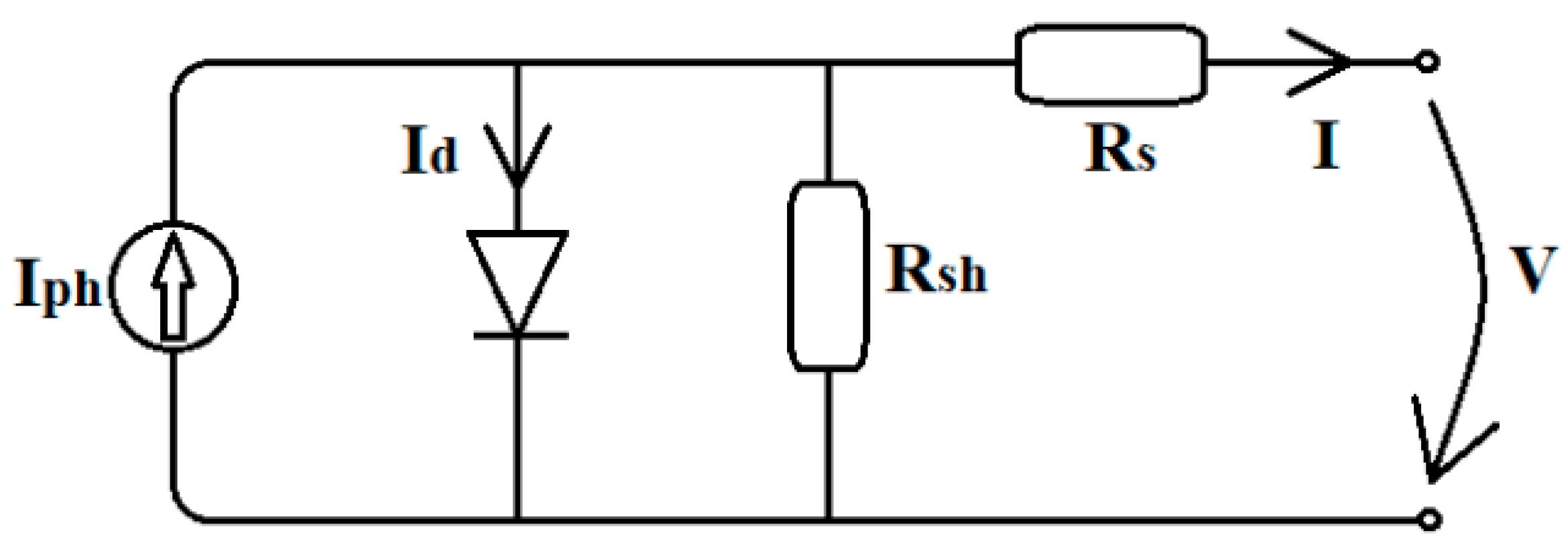
2. Mathematical Model of the Photovoltaic Panel

PV cell dynamics are minimal and, therefore, this paper uses only the nonlinear stationary expressions that serve as the base for the voltage–power and voltage–current characteristics for a specified pair of solar irradiance and temperature. It is appropriate to disregard the cell dynamics since the dynamics could be present only because of the capacitive nature intrinsic to a PV cell, which is minute, as proven in [51]. This paper uses an equivalent circuit for a photovoltaic setup [3] to determine the mathematical expressions, as shown in Figure 1. The model comprises one diode that appropriately emulates system behaviour, where the current source is affected by solar radiation and cell temperature. To emulate the semiconductor PN junction, a diode is placed in parallel with the current source. Moreover, a shunt resistor (Rsh) is placed in parallel with the cell, while another resistor is connected in series (Rs), which regulates the output current. This algorithm may be employed for a two-diode model, if necessary, but the gain in precision is not considerable.
Beginning with the equivalent circuit, mathematical model (1) is obtained, where the PV panel comprising N number of cells is fully represented by considering it as the sum of its cells connected in series. It may be possible to consider parallelly connected cells; however, it is rare in real scenarios.
I = I p h I 0 ( e q ( V + I R s ) a K T N s 1 ) V + I R s R s h
The first term is the photovoltaic current and is described as in (2).
I p h = G I S C + K i ( T T S T C ) G S T C
Table 1 specifies the parameters used in the system expression. Lastly, the diode saturation current is specified using expression (3).
I 0 = I S C + K i ( T T S T C ) e q [ V O C + K v ( T T S T C ) ] a K T N S 1
These expressions form the basis for the system under study, where there are fundamental nonlinearities introduced by the diode. Table 1 also specifies the characteristics of the PV panel that was employed to conduct the simulations (Maximum power of 325 W).
Solar irradiance of 1000 W/m2 and 25 °C temperature are considered the standard conditions under which the PV characteristics are specified.

3. Maximum Power Point Tracking Method

To sustain the maximum generated energy for every load value and external condition variable, the MPPT is of considerable significance. The principle on which MPPT architecture operates is based on calculating the necessary optimal value for the photovoltaic panel. The obtained optimal value is then sent as a reference to a control block that is responsible for the regulation of a DC/DC converter. Figure 2 depicts the synthesis of this. On the contrary, this architecture is not the only one that is implemented in practice. There exist several architectures that involve the stationary PV model within the DC/DC converter’s controller. However, these solutions are not recommended as they cause complications in the control algorithm, thereby decreasing the system′s sturdiness.
The main focus of this paper is the optimiser block, which includes the application of an optimisation algorithm. In general, this block is implemented with non-model-based methodologies (neural networks, P&O, etc.), as highlighted in the Introduction. The key benefit of the P&O approach is that it is simple and conveniently adaptable and applicable to various situations. However, it has its drawbacks that include lack of precision and presence of oscillations around the solution, where the oscillations have the tendency to propagate towards the controller and then to the remaining system. On the other hand, neural networks offer greater precision at the cost of increased computation time to readapt the model as per the requirements.
A group of characteristic curves is plotted in Figure 3 to validate and elaborate the correlation among voltage, current, power and external parameters. The different conditions under which the curves are plotted are as: for a temperature of 30 °C and solar radiation of 800 W/m2; for a temperature of 40 °C and solar radiation of 600 W/m2; and for a temperature of 15 °C and solar radiation of 1000 W/m2. The resulting correlation apparently appears as nonlinear.

3.1. Defining the Optimisation Problem

The literature mentions the development of various MPPT techniques regarding PV systems [52]. These techniques are different in numerous features, i.e., convergence quality, simplicity, additional equipment required, implementation manner and cost, as well as other features. For instance, Open Circuit Voltage method (OCV) regards the observation in which the maximum power point’s voltage is in proximity of the open-circuit voltage, as well as the approximation of the voltage of the maximum point Vmpp via the nominal Voltage in open circuit (Voc). Applying OCV is not very complicated with regards to a linear approximation, Vmpp = k*Voc, but the key drawback is the need to perform regular measurement pertaining to open-circuit voltage, which also changes as per the environmental parameters. In this case, it is important to bring in a static switch for the PV array in series in order to open the circuit; the working principle Short-Circuit Current method (SCC) is the same as that of the previous method, in that it allows approximation of maximum operating current Impp and the short-circuit current Isc. In fact, Impp is regarded to be proportional with that of the short-circuit current Isc that is exposed to different conditions pertaining to irradiance level as well as temperature, Impp = k*Isc. The drawback here is that this algorithm needs measurements pertaining to the current Isc and to get this measurement, it is important to bring in a static switch that is parallel with the PV array, so that short-circuit conditions can be created. Particularly for practical applications, it is suggested to use the P&O because of its simple logic of use. Employing P&O to determine MPP results in oscillations near the extreme point, and, when there are rapid variations pertaining to the intensity of solar radiation, it could result in MPP tracking in a different direction that is incorrect; the Incremental Conductance method (IncCond) involves tracking of the value pertaining to the power derivative with regards to the voltage. Different from the previous P&O, it does not involve oscillations pertaining to the operation or mis-tracking, but it would require more resources and could also impact the frequency pertaining to the current as well as the alternative voltage created. The popularity of the last two methods is high; however, their drawbacks include slow response towards rapid variations of the solar radiation, tracking in the incorrect direction and oscillations surrounding the MPP. The model-based methods of MPPT systems are deemed more efficient for formulating robust algorithms. In this context, our paper puts forward a new method that considers the gradient techniques to identify MPP based on a nonlinear optimisation problem that includes implicit equality restrictions.
The optimisation problem that must be mitigated is expressed as a maximisation of the photovoltaic power with regards to the current as well as voltage (I and V), wherein the equality constraint is g(I,V) = 0
{ max I , V [ P ( I , V ) ] g ( I , V ) = 0
where
{ P ( I , V ) = I V g ( I , V ) = I p h I 0 ( e q ( V + I R s ) a K T N s 1 ) V + I R s R s h I
For solving such an issue, the Lagrangian dual problem has been developed.

3.2. Lagrangian Dual Problem

This approach has already been exploited in some of the papers as mentioned in [27]. The dual problem that can be seen in (5) can be represented as:
L = I V + λ [ I p h I 0 ( e q ( V + I R s ) a K T N s 1 ) V + I R s R s h I ]
wherein λ is the Lagrange multiplier. As it is recognised, this suggests the resolution pertaining to the system of equations:
{ L λ = 0 L I = 0 L V = 0
As solving this is not as simple as perceived, the specialised literature mentions applying various methodologies. For instance, even after the Lagrange multiplier is substituted in the other two equations which are now treated as the new optimisation criterion, it will result in an equation that includes fractions; this gives rise to problems in its resolution. Our proposed approach suggests directly writing a quadratic minimisation criterion to solve this:
min I , V , λ [ ( L λ ) 2 + ( L I ) 2 + ( L V ) 2 ]
A Newton–Raphson method can be used to solve this optimisation issue, yet it would be very complicated to compute the Hessian. A Cauchy gradient method would be the first appropriate solution. Directly applying Cauchy with a fixed step would not result in a universal step that would function with any external condition, and calculation of a variable step directly would also be difficult due to the nonlinear form pertaining to the criterion function (8). The next subsection shows the solution employed here.

3.3. Optimisation Solution

The out forward optimisation algorithm for minimisation of (8) is one of the innovations in this paper, which can be seen as a hybrid between the NAG and the Adadelta method [49] that allows determining an optimal variable maximum step size.
The Algorithm 1 can be synthesised as below:
Algorithm 1. Out forward Optimisation for Minimisation.
1 .   Initialization   of   the   optimization   variable :     x = [ I ,   V ,   λ ] T 2 .   Initialize   other   variables :   Eg 2 = 0 3 ;   ε = 10 8 ;   RMS D x = 0 3 ;   EDx 2 = 0 3 ;   θ = 0 3 ; μ 1 = 0.97 ;   μ 2 = 0.9 3 .   while   ( stop   condition ) 3 . 1 .   x p r e d i c t = x μ 1 θ 3.2 .   Grad = gradient ( x p r e d i c t ) 3 . 3 .   E g 2 = μ 2 E g 2 + ( 1 μ 2 ) Grad 2 3.4 .   RMS g 2 = E g 2 + ε 3.5 .   α = 0 . 5 R M S D x RMS g 2 3.6 .   θ = μ 1 θ + α Grad 3 . 7 .   x = x - θ 3.8 .   E D x 2 = μ 1 E D x 2 + ( 1 μ 1 ) θ 2 3.9 .   R M S D x = E D x 2 + ε
The values corresponding to the gradient of the quadratic objective Function (8) (named here as J), with regards to I, V and λ, are described in the Appendix A. Since the optimisation variable x is regarded as a vector possessing three elements, all the mathematical operations have been executed term by term, i.e., the square operation returns a vector of three elements, each term squared, and the same for the square root and division.
The Eg2 and EDx2 parameters signify an exponentially decaying average pertaining to the squared gradients values as well as squared advancement step θ, respectively, up until the current time. We employ the RMS values as implied in the Adadelta algorithm. Parameters μ could be described as the decay parameters that share similarity with the momentum coefficients of the momentum gradient methods. These values need to be selected appropriately in an experimental way, with a value near 0.9.
It needs to be noted that the Gradient is computed for a predicted value corresponding to the optimisation variable x (I, V, λ) and should be handled with care, as recommended from the NAG method.
The constant ε is selected as a small value to guarantee numerical stability pertaining to the algorithm.
The stopping condition is selected as a sum of its last three norms calculated between the last advancement step and the current advancement step θ.

4. Validation in Simulation

Simulation was used in two steps for validation: firstly, the optimiser was examined without control and, secondly, within the MPPT architecture that includes a DC/DC converter, the adjacent controller and a DC motor as load.

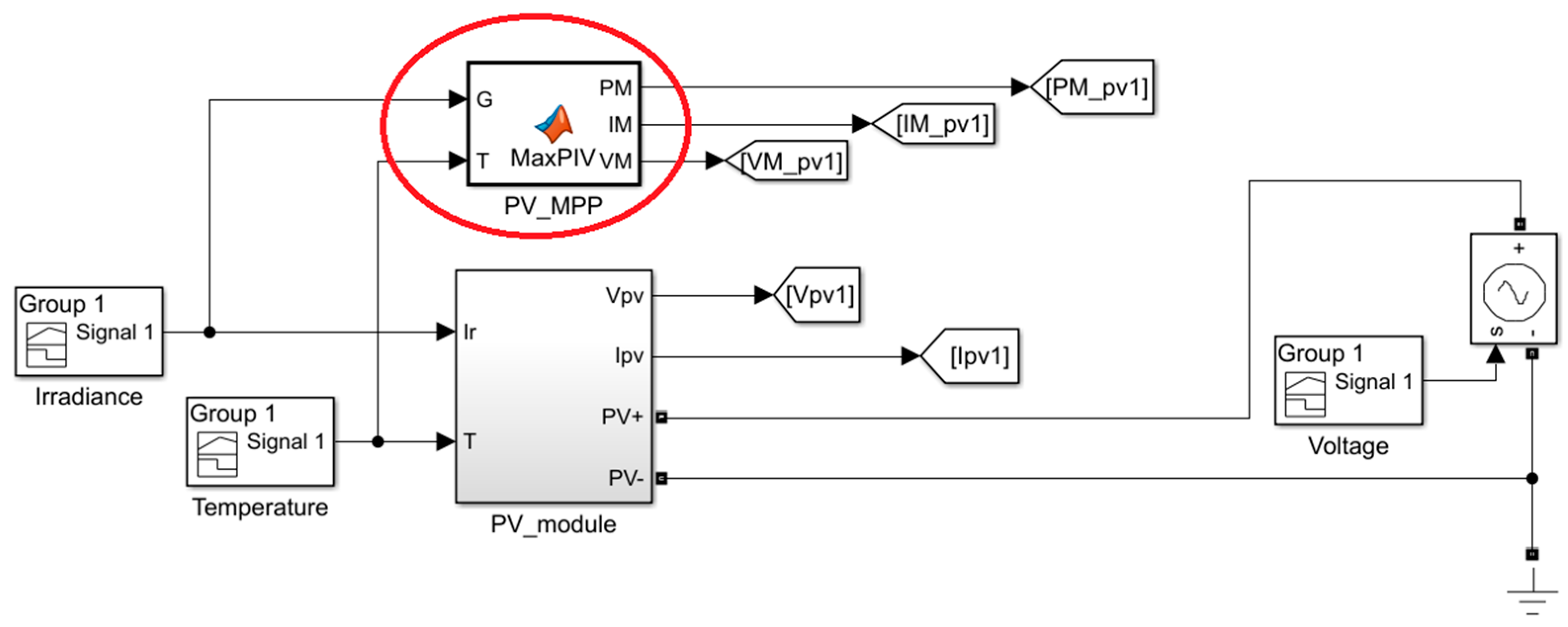
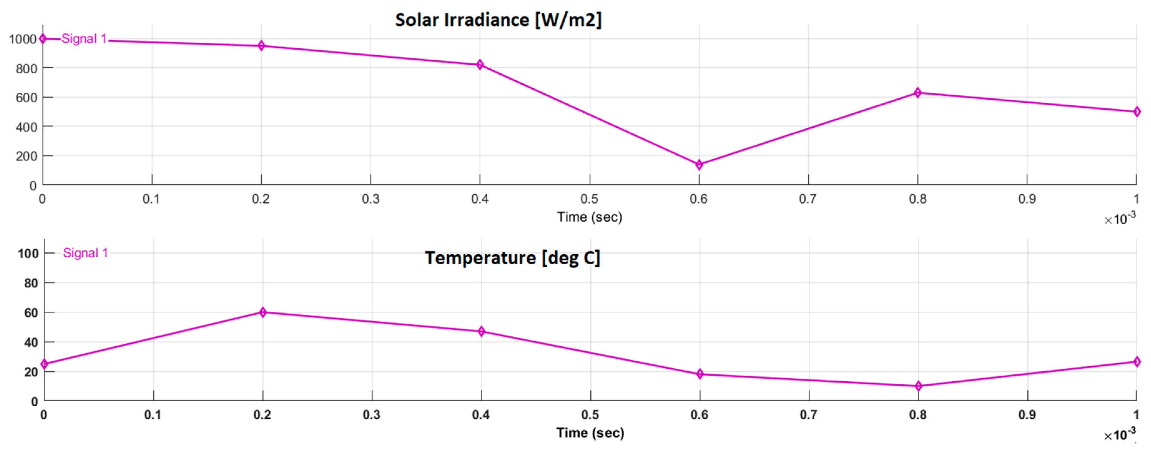
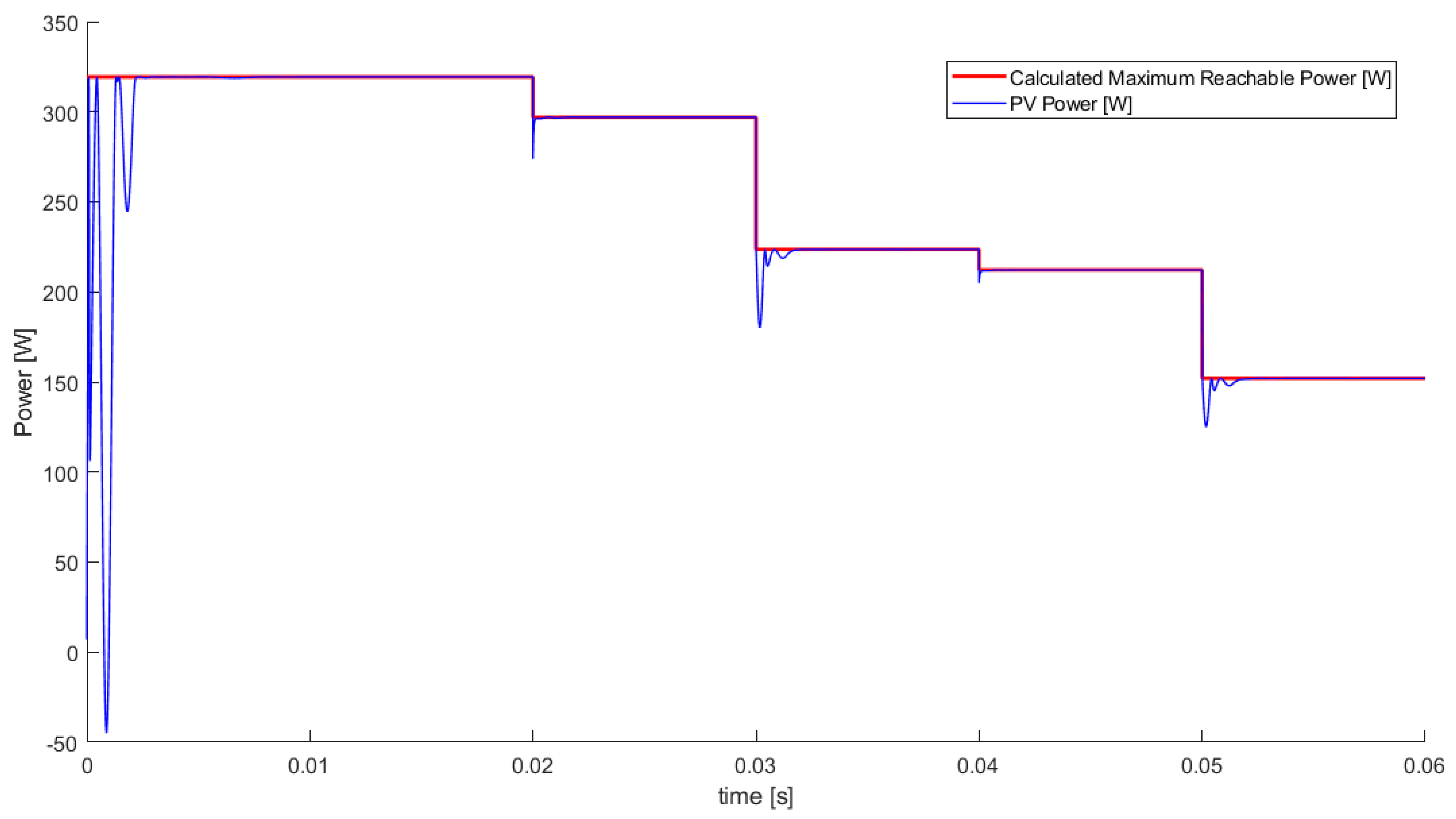
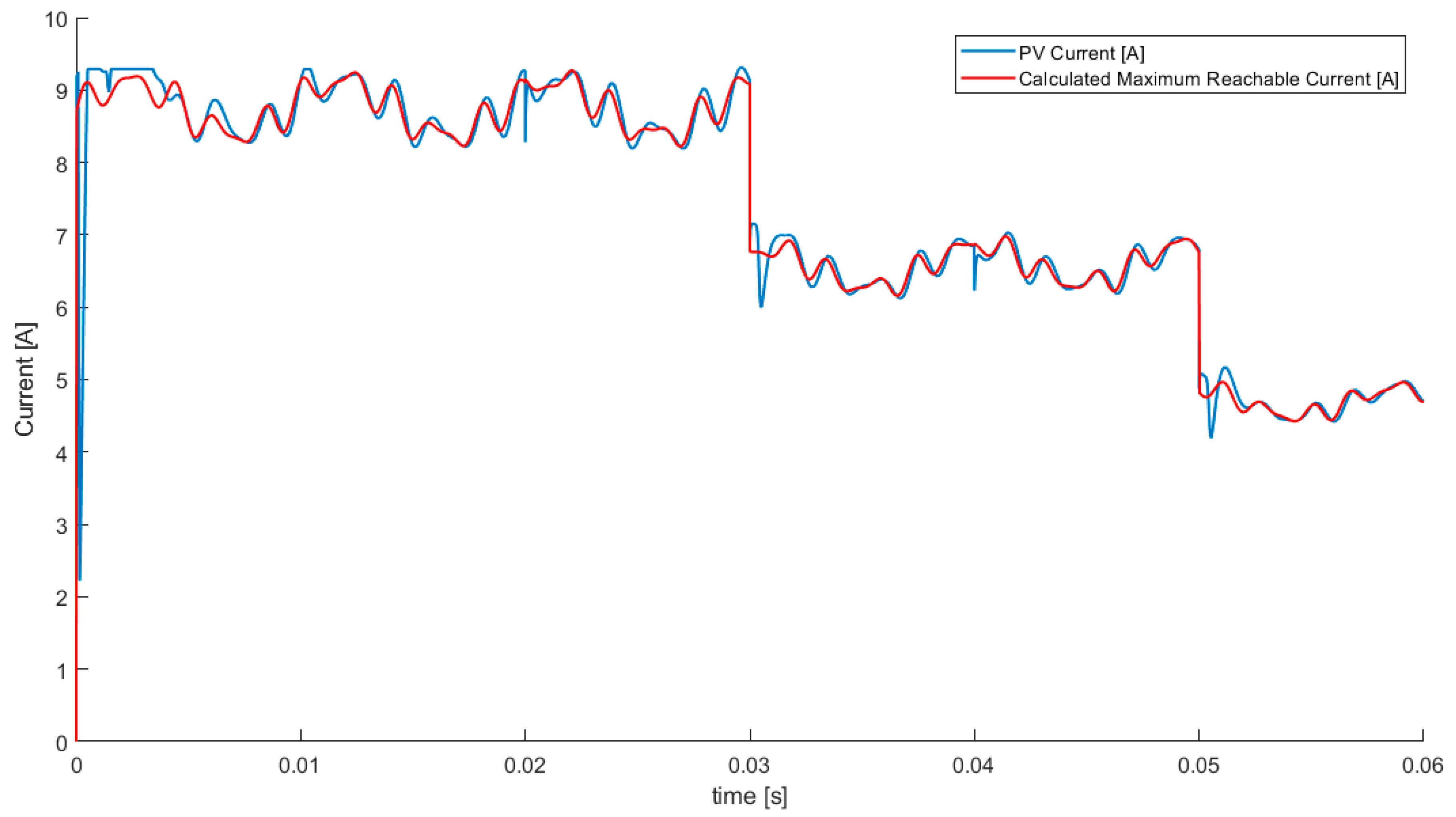
4.1. Validation of the Optimiser Block without Control

To confirm the method’s efficiency, tests are carried out in simulation by changing ambient conditions. In Figure 4, a test scenario is demonstrated in simulation by employing Matlab/Simulink. The voltage was set to swing from 0 V towards the open circuit voltage. The optimiser block described earlier is represented by encircled block.
The varying test conditions are presented in Figure 5.
The results are depicted in Figure 6. Since the system is not being controlled, Figure 6a,b shows that the instantaneous voltage–current as well as voltage–power curves are in most cases smaller when compared with the maximum value. Red arrows show the curves’ dynamics. It is necessary to note here that the MPP detection algorithm performs satisfactorily even at the inflexion points, where computations are harder, a constraint that other methods suffer from.

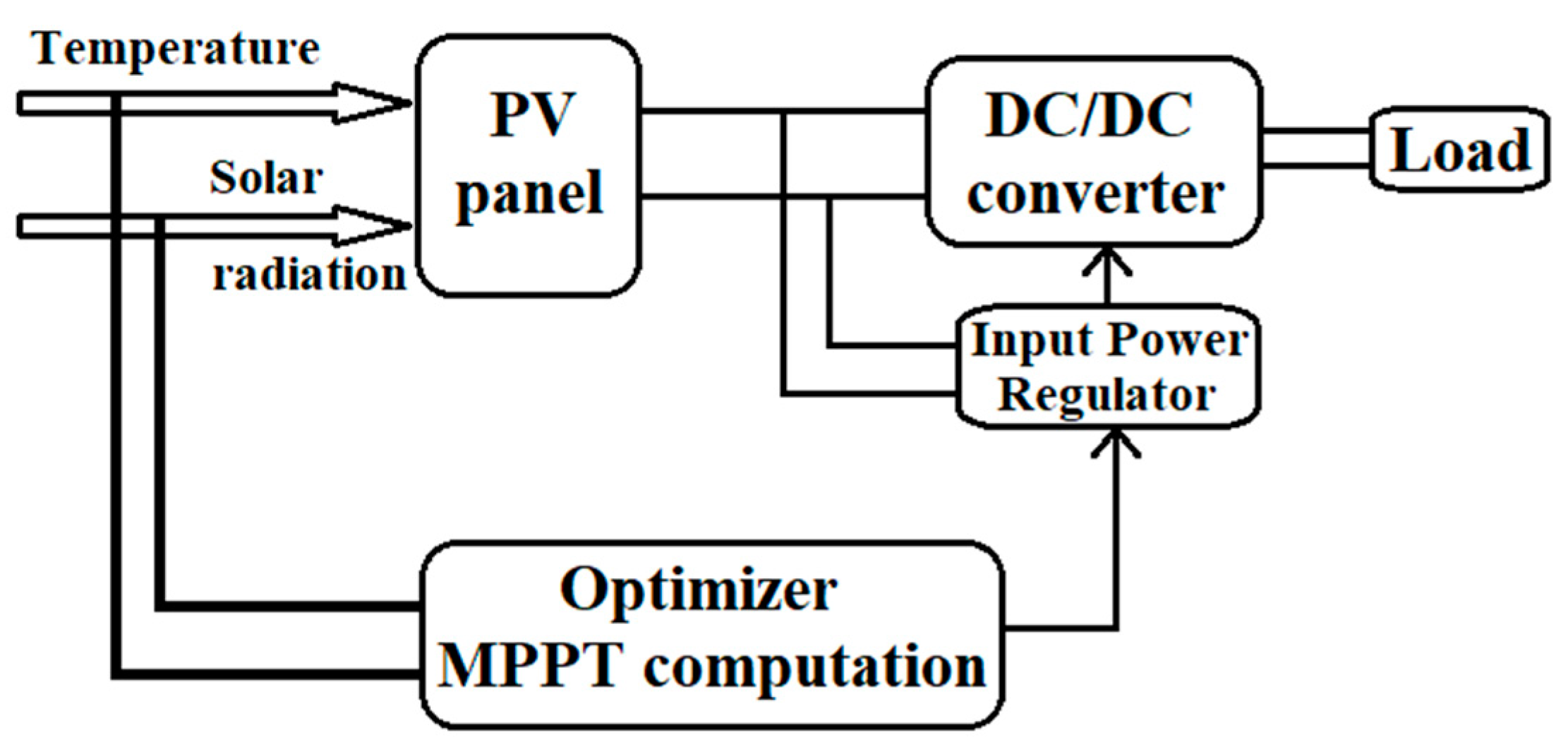
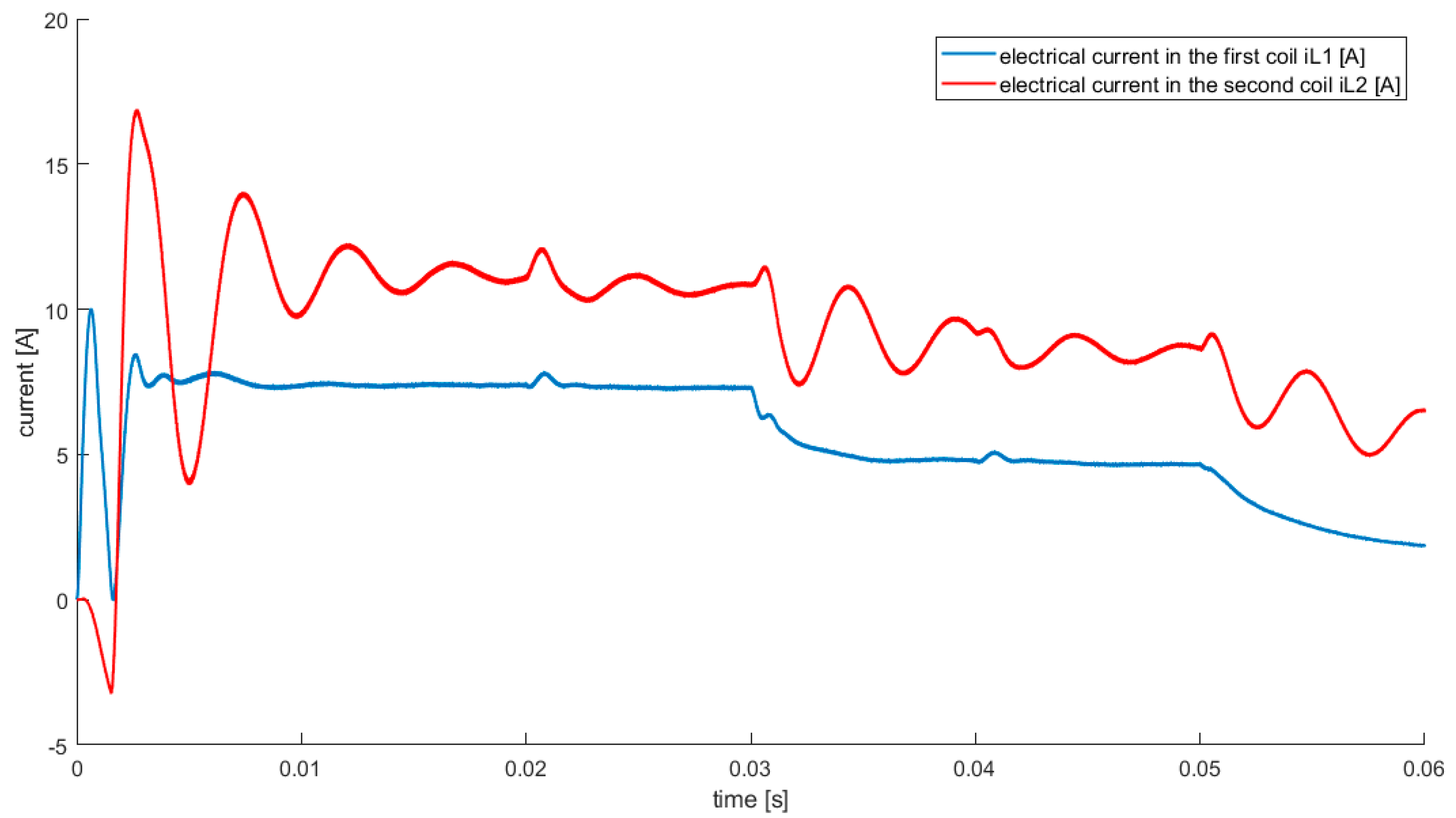
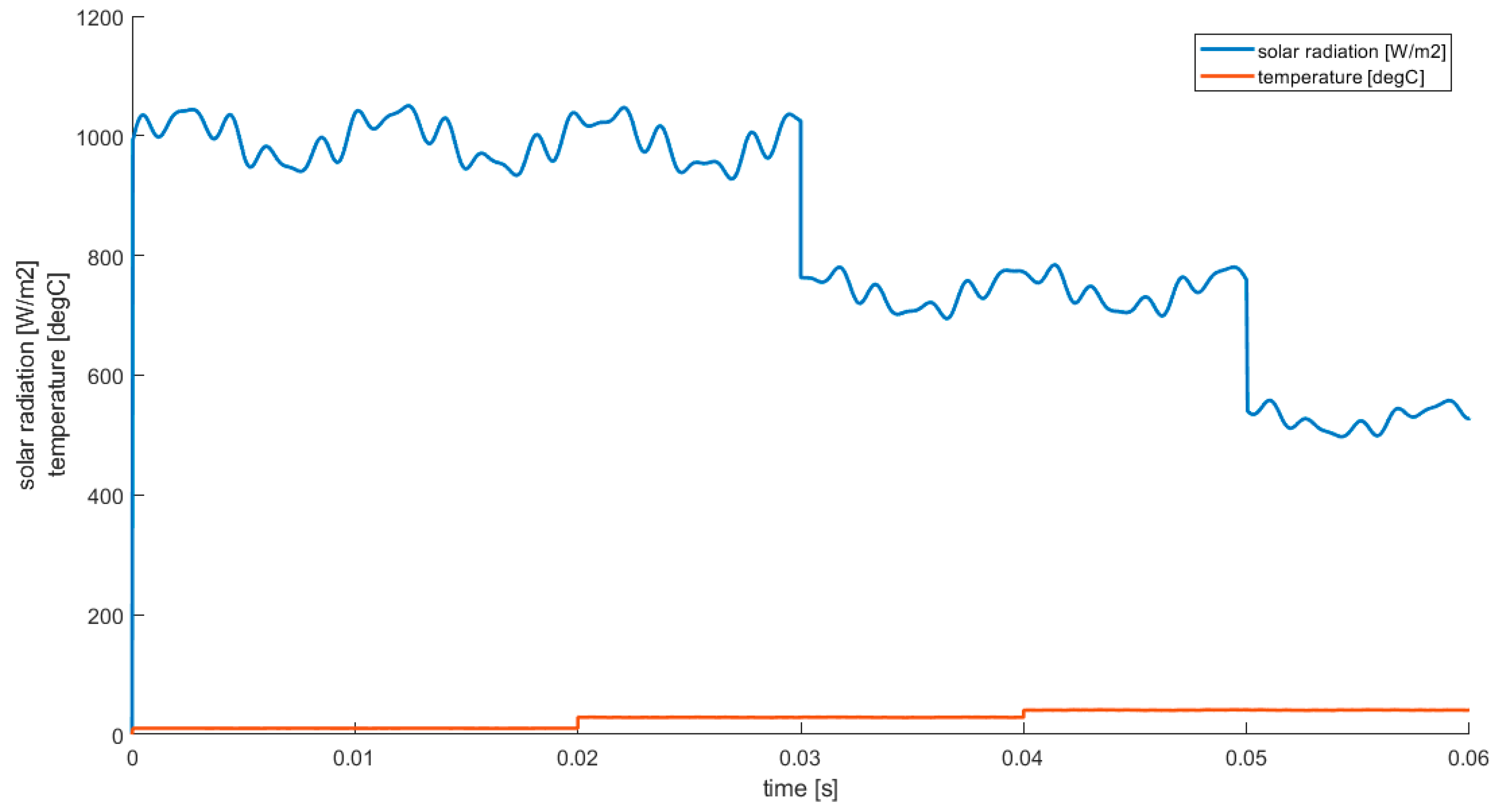
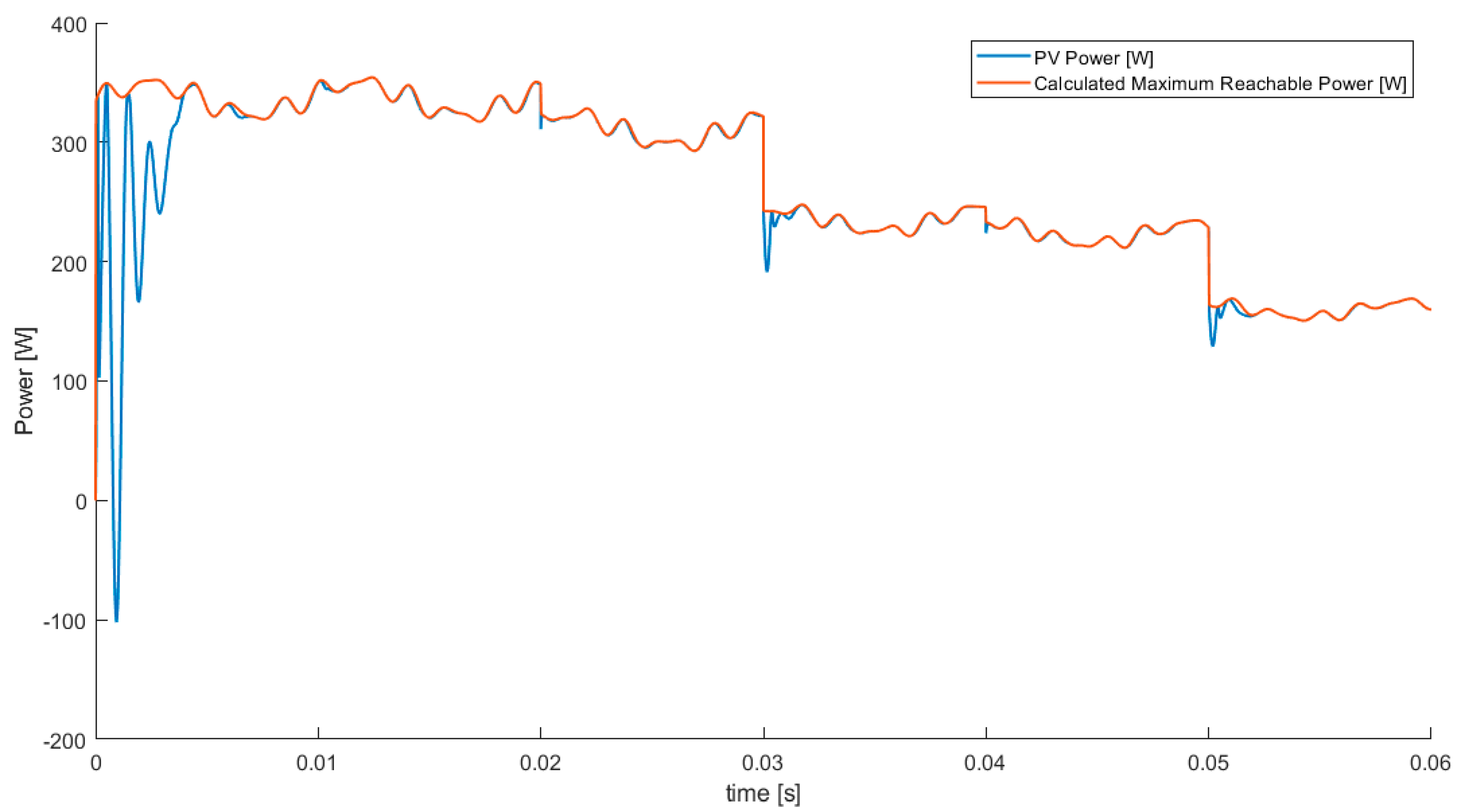
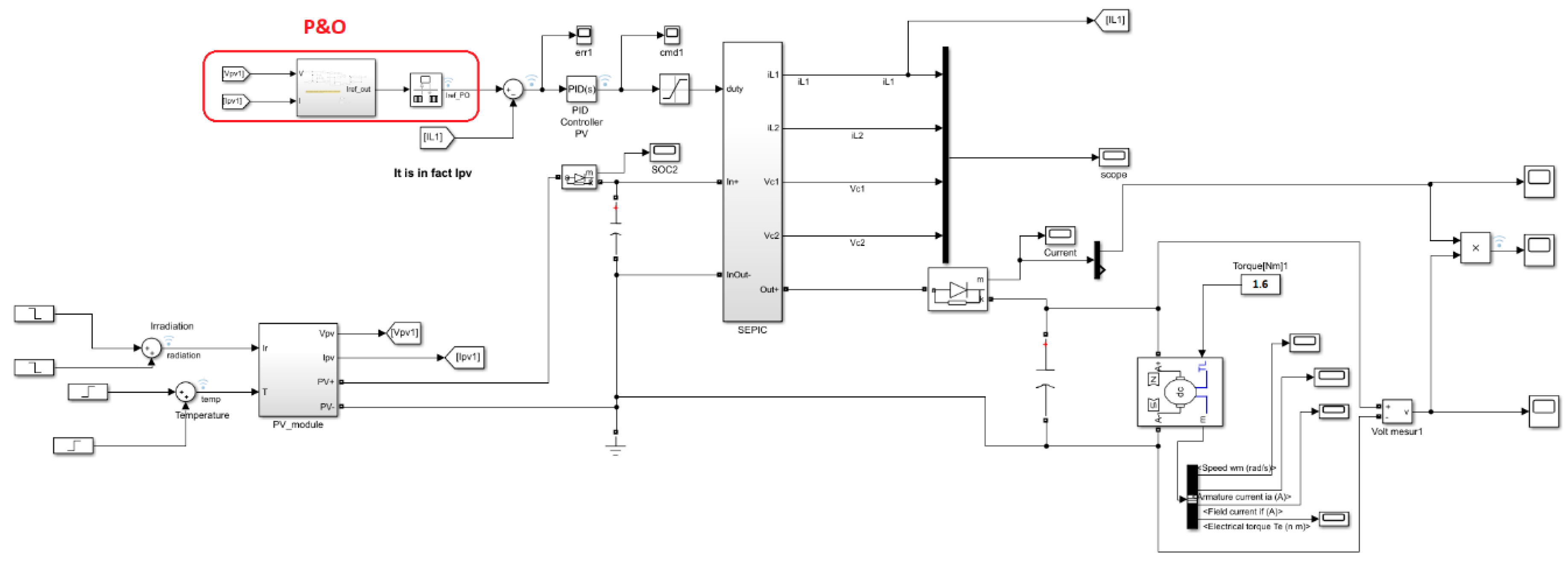
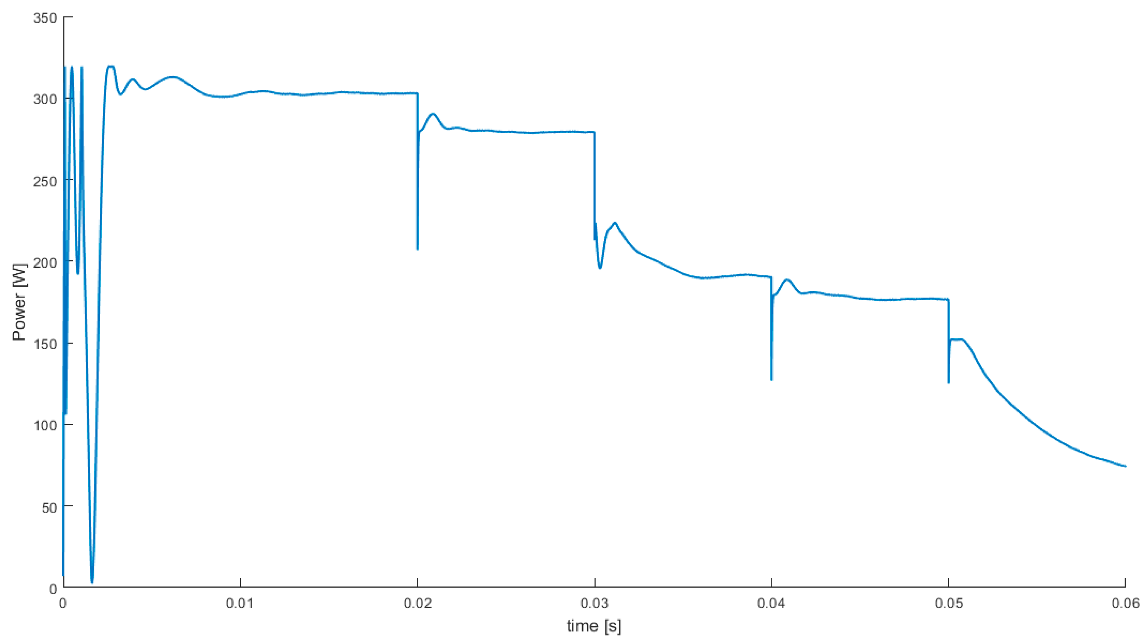
4.2. Validation of the Optimiser Block in an MPPT Control Architecture

Using the schematic architecture shown in Figure 2 as a basis, the simulation was equipped with a DC/DC converter so that the photovoltaic panel’s operating point can be moved to the maximum values determined by the Optimiser block.
The DC/DC converter selected was a SEPIC (Single Ended Primary Inductor Converter) which can lift as well as reduce the output voltage. The control process was performed on the input current, which is encircled in Figure 7.
The choice for the SEPIC is justified by the fact that it preserves the generality in varying consumers. This implies the designed method can be implemented within specified conditions where the optimal voltage can be higher or lower than the PV voltage. As such, from the different existing topologies of DC-DC converters that satisfy this constraint, the SEPIC architecture was selected, as it satisfies the requirement of continuous current at the input variable (since the controlled input is the current). This type of converter is widespread for power regulation applications. The circuit is in synchronous mode, signifying that there are two switches controlled in anti-phase. The chosen parameters for the converter are presented in Table 2.
The overall schematic is depicted in Figure 8. A capacitor of 20 μF was supplemented at the input of the converter for simulation purposes, not affecting the general behaviour of the photovoltaic panel. The selected load was a DC motor to simulate a more intricate consumer. The DC motor’s parameters are shown in Table 3. The sampling period in simulation was selected to be 3 10−8, in order to detect all the electrical system dynamics.
To control the current of the photovoltaic panel, a PI controller, in its ideal form, with an Integrator gain of 4000 and a Proportional gain of 0.1 was added. An advanced controller may be used; however, this was not the key aim of the present study. Furthermore, a set of tests was carried out to validate the solution. The results are shown for varying temperatures and solar radiations, representing five different regions that can be distinguished in Figure 9.
Figure 10 and Figure 11 illustrate, respectively, the dynamic behaviour of the generated power and the generated electric current over time. It can be seen in Figure 11 that, in particular moments, the current exceeds the maximal value, showing a minor overshoot. This is attainable since the PV voltage decreases during these moments, which signifies that the power is still lower than the maximum reachable value. The response stabilises at a maximum of 4 ms, which is a reasonable value.
The response observed during the first 2 ms is altered because the converter does not reach the nominal working conditions, as it has not entered a continuous conduction mode. Once these conditions are achieved, system stabilisation takes place at the maximum generated power. This can be seen in Figure 12, where the electric currents in both coils are presented. It is obvious that in the first milliseconds the coils’ currents are zero or negative.
Although the step response is a good indicator for the system’s response, as it is a persistent signal covering the significant part of the frequency spectrum, a set of perturbed signals was also added for the temperature and solar irradiance, as presented in Figure 13.
In Figure 14 and Figure 15, the system’s response is shown. Even with the highly oscillating input parameters, the optimisation algorithm that gives the maximum power point reference, as well as the whole architecture, manages to overcome the fluctuating inputs.
The current is shown in Figure 15, as it is the reference for the regulator.
Based on the results in Figure 6, where the optimisation algorithm is evaluated for a continuously varying range of external parameters, as well as the simulations presented in Figure 10 and Figure 11 without continuous oscillations and Figure 13 and Figure 14 with continuous oscillations, the architecture is concluded to be efficient in simulation.

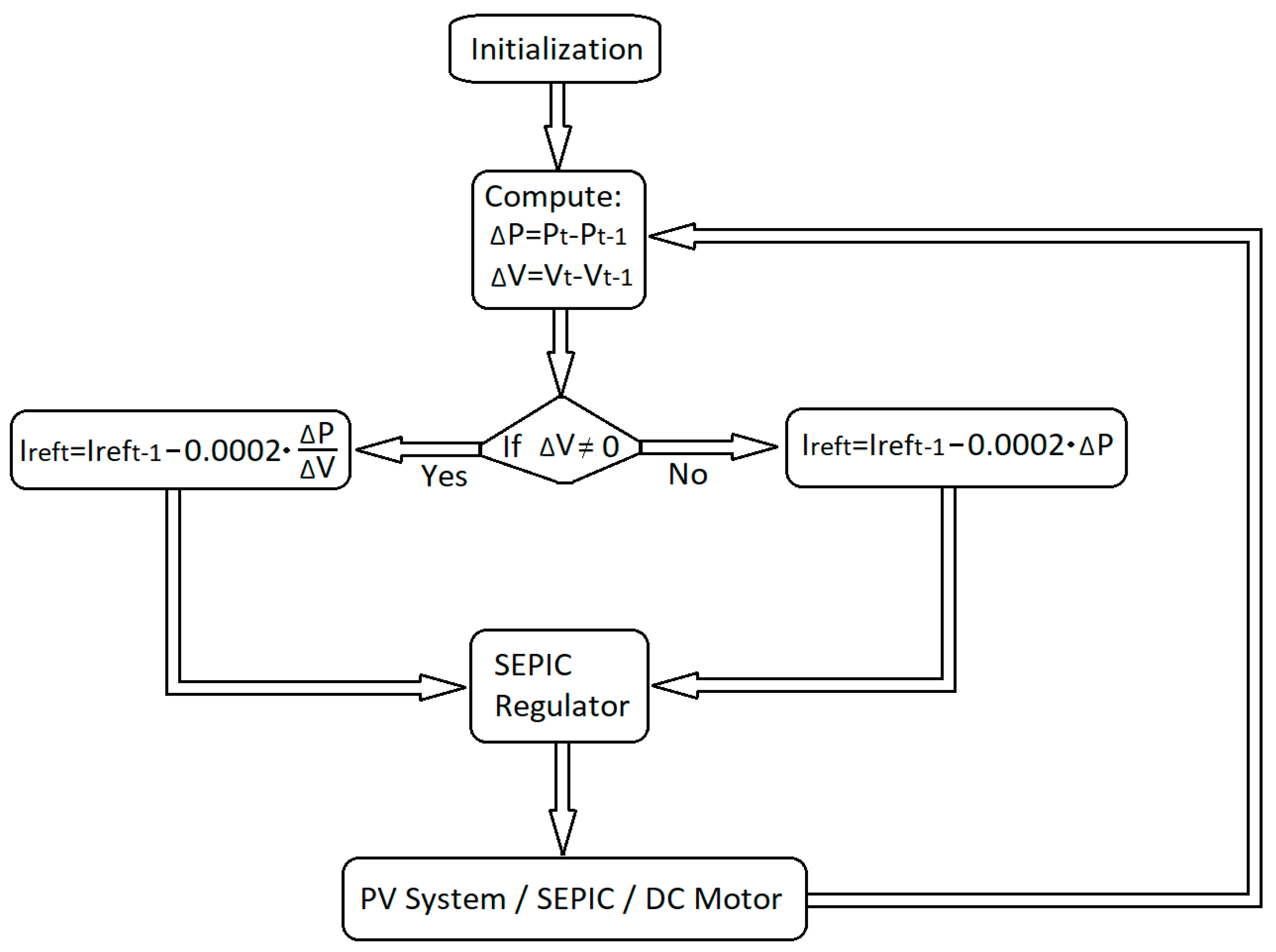
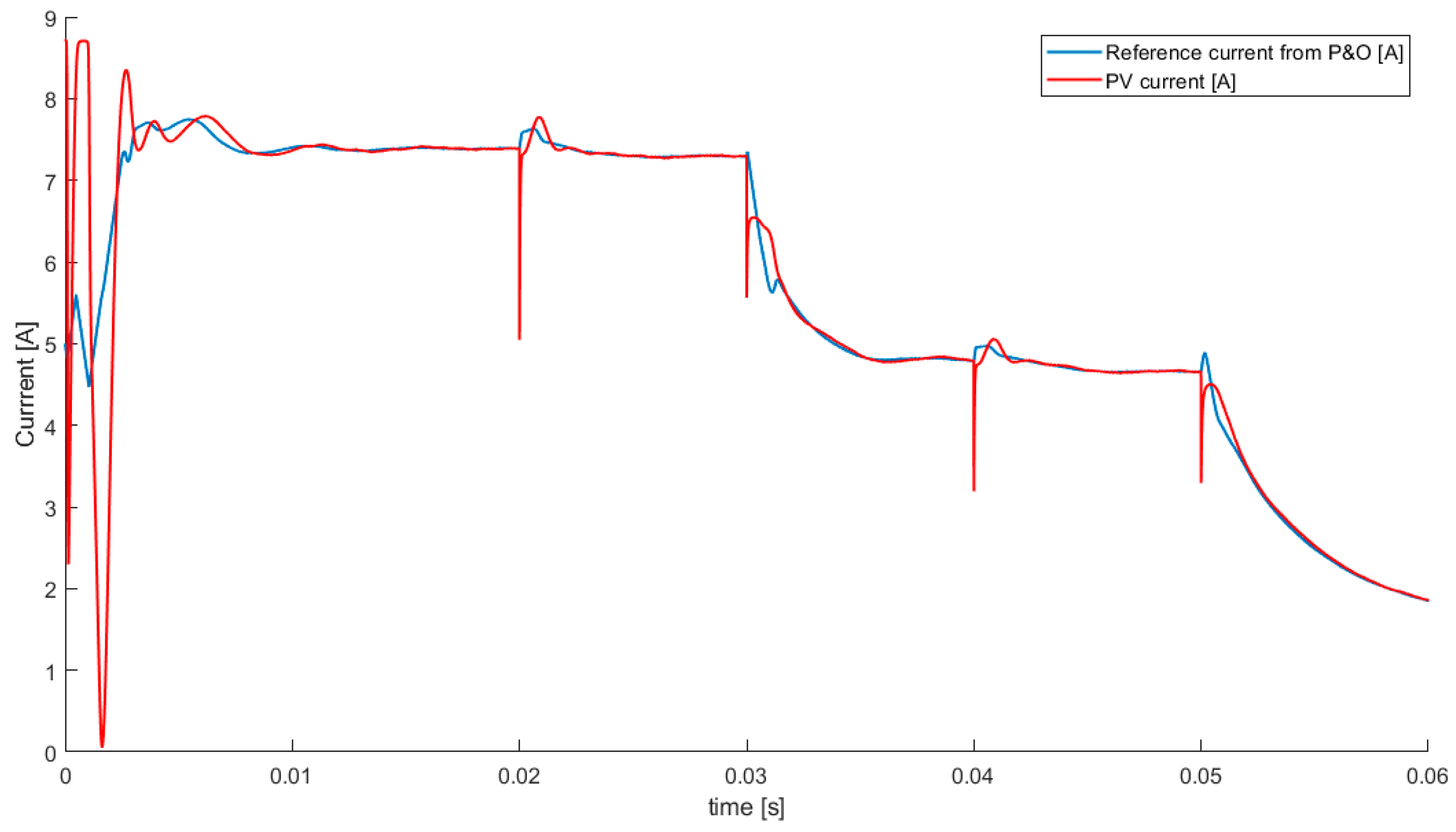
4.3. Comparative Study between the Proposed Architecture and a Classical P&O Approach

To better analyse the proposed solution, a comparative study was carried out with a conventional method, P&O. The P&O algorithm adapted to the investigated system in this work is presented synthetically in Figure 16. The sampling period was selected to be 10−7 s.
The implementation in simulation of the entire system architecture is presented in Figure 17.
To make a framework of a performance comparison, the system response is presented in Figure 18 and Figure 19, in the same way as previously illustrated for the designed method in this work. The system inputs variations are the ones presented in Figure 9.
It appears obviously that the system response in Figure 18 and Figure 19 is slower than the obtained response with the established method in this article. This was expected as the P&O approach is an iterative method, whereas the designed technique in this present work is a model-based method, calculating the maximum power point at each change in external parameters (temperature and solar radiation). The slower response weakness is quite obvious at Second 0.05 where it enables stabilisation when compared to the response in Figure 10.
The disadvantage generated by the slow response time of the P&O method is contrasted by its simplicity of implementation on an embedded platform.

5. Conclusions

The paper formulates a gradient-based optimisation algorithm that can be used to calculate the maximum power point for photovoltaic panels. This algorithm can also be incorporated into the MPPT control architecture. The paper utilises an optimisation algorithm that uses the NAG method for quickly determining the solution and skipping over local minima points, as well as the Adadelta method for estimating a varying step size. Moreover, the proposed gradient method calculates MPP by providing a solution to the nonlinear mathematical programming problem (NMP) expressed in (4) for the electrical power that solar systems generate. The solution of this problem is attained exploiting a numerical recursive strategy based on the associated Lagrange function of the stationary point. This point is associated with the Lagrange function and is a representative of the Vmpp voltage and Impp current for the point of maximum power generated. Based on the comparative performance study analysis presented in Section 3.1 and the case study in Section 4.3, it can be concluded that the proposed method, despite some additional calculation efforts, performs better than the P&O method, which is often recommended in practical applications. It has also superior performance compared to other methods. Furthermore, the proposed method removes the inconveniences associated with OCV and SCC techniques and does not need additional static switches and additional measurements. Alternatively, our method performs better than the P&O and IncCond procedures as it eliminates the disadvantages associated with slow responses to swift solar radiation and temperature variations. Furthermore, more accurate estimates of the MPP is ensured despite near oscillations and environment disturbances. Likewise, the proposed design scheme does not rely on the algorithm’s initialisation. Compared to other gradient methods, the final quadratic form of the optimisation problem that was implemented offers additional robustness to the designed solution in regards to different external conditions. Besides, the optimisation method used manages to jump over local minima that arise from the nonlinear form of the objective function.
The result of the qualitative comparative study has shown the satisfactory performance of the NAG algorithm in achieving swift convergence without affecting the accuracy in fixing the MPP.
A perspective of the current work is to implement the solution on a physical platform. As theoretical perspectives, the focus of further studies should be on analysing the effects of shading on the PV systems and how the method presented here can be adapted for this case. Furthermore, stochastic optimisation methods that include solar radiation and temperature as stochastic process variables are intended to be explored.

Author Contributions

S.C.O. proposed and validated the improved optimisation method. F.H. dealt with the control architecture as well as working on the state-of-the-art section. D.P. proposed the optimisation problem for the photovoltaic system. I.D. dealt with editing. H.J. and S.B.A. polished and reviewed the manuscript and R.A. helped in reviewing and reorganising the paper. Conceptualisation, S.C.O., F.H. and D.P.; Data curation, F.H. and S.C.O.; Formal analysis, D.P.; Investigation, H.J.; Methodology, D.P. and S.C.O.; Project administration, H.J.; Resources, I.D.; Software, S.C.O., I.D. and S.B.A.; Supervision, D.P.; Validation, F.H., H.J. and R.A.; Writing—original draft, S.C.O. and I.D.; and Writing—review and editing, F.H., S.C.O. and I.D. All authors have read and agreed to the published version of the manuscript.

Funding

This research received no external funding.

Conflicts of Interest

The authors declare no conflict of interest.

Abbreviations

MPPTMaximum Power Point Tracking
MPPMaximum Power Point
PVPhotovoltaic
NAGNesterov Accelerated Gradient
SEPICSingle Ended Primary Inductor Converter
IncCondIncremental conductance method
P&OPerturb and Observe
COPconstrained optimisation problem

Appendix A

Alpha = 1/(a*Ns*(K*T)/q); %T is in Kelvin
gradJdI = 4*I − 2*I01 − 2*Iph + (2*V)/Rsh − (2*lamb)/Rsh +…
2*I01*exp(alpha*(V + I*Rs)) + …
(2*I*Rs^2)/Rsh^2 − (2*I01*Rs)/Rsh + (4*I*Rs)/Rsh − (2*Iph*Rs)/Rsh + …
(2*Rs*V)/Rsh^2 − 2*I01*alpha*lamb*exp(alpha*(V + I*Rs)) +…
(2*I01*Rs*exp(alpha*(V + I*Rs)))/Rsh − 2*I01^2*Rs*alpha*exp(alpha*(V + I*Rs)) +…
2*I01^2*Rs*alpha*exp(2*alpha*(V + I*Rs)) +…
2*I01^2*Rs^3*alpha^3*lamb^2*exp(2*alpha*(V + I*Rs)) +…
2*I01*I*Rs*alpha*exp(alpha*(V + I*Rs)) − 2*I01*Iph*Rs*alpha*exp(alpha*(V + I*Rs)) +…
2*I01*Rs^2*alpha^2*lamb^2*exp(alpha*(V + I*Rs)) +…
2*I01^2*Rs*alpha^3*lamb^2*exp(2*alpha*(V + I*Rs)) +…
(2*I01*Rs*alpha^2*lamb^2*exp(alpha*(V + I*Rs)))/Rsh +…
(2*I01*Rs*V*alpha*exp(alpha*(V + I*Rs)))/Rsh -…
2*I01*I*Rs*alpha^2*lamb*exp(alpha*(V + I*Rs)) +…
(2*I01*Rs^3*alpha^2*lamb^2*exp(alpha*(V + I*Rs)))/Rsh +…
(2*I01*I*Rs^2*alpha*exp(alpha*(V + I*Rs)))/Rsh -…
2*I01*Rs^2*V*alpha^2*lamb*exp(alpha*(V + I*Rs));
gradJdV = 2*V − 2*lamb − (2*I01)/Rsh + (2*I)/Rsh − (2*Iph)/Rsh + (2*V)/Rsh^2 +…
(2*I01*exp(alpha*(V + I*Rs)))/Rsh − 2*I01^2*alpha*exp(alpha*(V + I*Rs)) +…
2*I01^2*alpha*exp(2*alpha*(V + I*Rs)) + (2*I*Rs)/Rsh^2 − (2*Rs*lamb)/Rsh +…
2*I01*I*alpha*exp(alpha*(V + I*Rs)) − 2*I01*Iph*alpha*exp(alpha*(V + I*Rs)) +…
2*I01^2*alpha^3*lamb^2*exp(2*alpha*(V + I*Rs)) +…
2*I01^2*Rs^2*alpha^3*lamb^2*exp(2*alpha*(V + I*Rs)) +…
2*I01*Rs*alpha^2*lamb^2*exp(alpha*(V + I*Rs)) -…
2*I01*Rs*alpha*lamb*exp(alpha*(V + I*Rs)) +…
(2*I01*alpha^2*lamb^2*exp(alpha*(V + I*Rs)))/Rsh +…
(2*I01*V*alpha*exp(alpha*(V + I*Rs)))/Rsh -…
2*I01*I*alpha^2*lamb*exp(alpha*(V + I*Rs)) +…
(2*I01*I*Rs*alpha*exp(alpha*(V + I*Rs)))/Rsh -…
2*I01*Rs*V*alpha^2*lamb*exp(alpha*(V + I*Rs)) +…
(2*I01*Rs^2*alpha^2*lamb^2*exp(alpha*(V + I*Rs)))/Rsh;
gradJdL = 2*lamb − 2*V − (2*I)/Rsh + (2*lamb)/Rsh^2 + (2*Rs^2*lamb)/Rsh^2 − (2*Rs*V)/Rsh +…
(4*Rs*lamb)/Rsh + 2*I01^2*alpha^2*lamb*exp(2*alpha*(V + I*Rs)) -…
2*I01*I*alpha*exp(alpha*(V + I*Rs)) -…
2*I01*Rs*V*alpha*exp(alpha*(V + I*Rs)) + 4*I01*Rs*alpha*lamb*exp(alpha*(V + I*Rs)) +…
2*I01^2*Rs^2*alpha^2*lamb*exp(2*alpha*(V + I*Rs)) +…
(4*I01*alpha*lamb*exp(alpha*(V + I*Rs)))/Rsh +…
(4*I01*Rs^2*alpha*lamb*exp(alpha*(V + I*Rs)))/Rsh;

References

  1. Khaehintung, N.; Sirisuk, P.; Kunakorn, A. Grid-connected photovoltaic system with maximum power point tracking using self-organizing fuzzy logic controller. In Proceedings of the Tencon 2005 IEEE Region 10 Conference, Melbourne, VIC, Australia, 21–24 November 2005. [Google Scholar]
  2. Salas, V.; Olias, E.; Barrado, A.; Lazaro, A. Review of the maximum power point tracking algorithms for stand-slone photovoltaic systems. Sol. Energy Mater. Sol. Cells 2006, 90, 1555–1578. [Google Scholar] [CrossRef]
  3. Mrabti, T.; El Ouariachi, M.; Yaden, M.; Kassmi, K.; Kassmi, K. Characterization and modeling of electrical performance of the photovoltaic panels and system. J. Electr. Eng. Theory Appl. 2010, 1, 100–110. [Google Scholar]
  4. Jerbi, H. Design and performance analysis of a PV solar powered water pumping system. Int. J. Adv. Appl. Sci. 2017, 4, 127–132. [Google Scholar] [CrossRef] [Green Version]
  5. El Ouariachi, M.L.; Mrabti, T.; Tidahf, B.; Kassmi, K.; Kassmi, K. Regulation of the electric power provided by the panels of the photovoltaic system. Int. J. Phys. Sci. 2009, 4, 294–309. [Google Scholar]
  6. Esram, T.; Chapman, P.L. Comparison of Photovoltaic Array Maximum Power Point Tracking Techniques. IEEE Trans. Energy Convers. 2007, 22, 439–449. [Google Scholar] [CrossRef] [Green Version]
  7. Shraif, M.F. Optimisation et Mesure de Chaîne de Conversion D’énergie Photovoltaïque en Energie Electrique. Ph.D. Thesis, Université Paul Sabatier, Toulouse, France, 2002. [Google Scholar]
  8. Hussein, K. Maximum photovoltaic power tracking: An algorithm for rapidly changing atmospheric conditions. IEEE Proc. Gener. Transm. Distrib. 1995, 142, 59–64. [Google Scholar] [CrossRef]
  9. Cocconi, A.; Rippel, W. Lectures from GM Sun Racer Case History, Lecture 3-1: The Sun Racer Power Systems’; Number M-101; Society of Automotive Engineers: Warrendale, PA, USA, 1990. [Google Scholar]
  10. Veerachary, M.; Senjyu, T.; Uezato, K. Neural-network-based maximum-power-point tracking of coupled-inductor interleaved-boost-converter-supplied pv system using fuzzy controller. IEEE Trans. Ind. Electron. 2003, 50, 749–758. [Google Scholar] [CrossRef] [Green Version]
  11. Bahgat, A.B.G.; Helwa, N.H.; Ahmad, G.E.; El Shenawy, E.T. Maximum power point tracking controller for PV systems using neural networks. Renew. Energy 2005, 30, 1257–1268. [Google Scholar] [CrossRef]
  12. Swrup, T.; Ansari, A. Maximum power point tracking method for multiple photovoltaic systems. Res. J. Chem. Sci. 2012, 2, 69–77. [Google Scholar]
  13. Masoum, M.A.S.; Dehbonei, H.; Fuchs, E.F. Theoretical and experimental analysis of photovoltaic systems with voltage and current-based maximum power-point tracking. IEEE Trans. Energy Conver. 2002, 17, 514–522. [Google Scholar] [CrossRef] [Green Version]
  14. Mellit, A.; Kalogirou, S. Artificial intelligence techniques for photovoltaic applications: A review. Prog. Energy Combust. Sci. 2008, 34, 574–632. [Google Scholar] [CrossRef]
  15. Lalouni, S.; Rekioua, D.; Rekioua, T.; Matagne, E. Fuzzy logic control of stand-alone photovoltaic system with battery storage. J. Power Sources 2009, 193, 899–907. [Google Scholar] [CrossRef]
  16. Salas, V.; Olías, E.; Barrado, A.; Lázaro, A. New algorithm applied to maximum power point tracking without batteries. In Proceedings of the 21st European Photovoltaic Solar Energy Conference, Dresden, Germany, 4–8 September 2006. [Google Scholar]
  17. Rodriguez, C.; Amaratunga, G.A.J. Analytic Solution to the Photovoltaic Maximum Power Point Problem. IEEE Trans. Circuits Syst. I Regul. Pap. 2007, 54, 2054–2060. [Google Scholar] [CrossRef]
  18. Chung, H.S.-H.; Tse, K.; Hui, S.; Mok, C.; Ho, M. A novel maximum power point tracking technique for solar panels using a SEPIC or cuk converter. IEEE Trans. Power Electron. 2003, 18, 717–724. [Google Scholar] [CrossRef]
  19. Femia, N.; Petrone, G.; Spagnuolo, G.; Vitelli, M. Optimization of Perturb and Observe Maximum Power Point Tracking Method. IEEE Trans. Power Electron. 2005, 20, 963–973. [Google Scholar] [CrossRef]
  20. Tung, Y.M.; Hu, A.P.; Nair, N.K. Evaluation of Micro Controller Based Maximum Power Point Tracking Methods using dSPACE Platform. In Proceedings of the Australasian Universities Power Engineering Conference (AUPEC’06), Melbourne, VIC, Australia, 10–13 December 2006. [Google Scholar]
  21. Sera, D.; Máthé, L.; Kerekes, T.; Spataru, S.; Teodorescu, R. On the Perturb-and-Observe and Incremental Conductance MPPT Methods for PV Systems. IEEE J. Photovoltaics 2013, 3, 1070–1078. [Google Scholar] [CrossRef]
  22. Hadji, S.; Gaubert, J.; Krim, F. Maximum Power Point Tracking (MPPT) for photovoltaic systems using open circuit voltage and short circuit current. In Proceedings of the 3rd International Conference on Systems and Control, Algiers, Algeria, 29–31 October 2013; pp. 87–92. [Google Scholar]
  23. Zakzouk, N.E.; AAbdelsalam, A.K.; Helal, A.; Williams, B.W. Modified variable-step incremental conductance maximum power point tracking technique for photovoltaic systems. In Proceedings of the 39th Annual Conference of the IEEE Industrial Electronics Society (IECON), Vienna, Austria, 10–13 November 2013; pp. 1741–1748. [Google Scholar]
  24. Femia, N.; Granozio, D.; Petrone, G.; Spagnuolo, G.; Vitelli, M. Predictive & Adaptive MPPT Perturb and Observe Method. IEEE Trans. Aerosp. Electron. Syst. 2007, 43, 934–950. [Google Scholar]
  25. Femia, N.; Lisi, G.; Petrone, G.; Spagnuolo, G.; Vitelli, M. Distributed maximum power point tracking of photovoltaic arrays: Novel approach and system analysis. IEEE Trans. Ind. Electron. 2008, 55, 2610–2621. [Google Scholar] [CrossRef] [Green Version]
  26. Khabou, H.; Souissi, M.; Aitouche, A. MPPT implementation on boost converter by using T–S fuzzy method. Math. Comput. Simul. 2020, 167, 119–134. [Google Scholar] [CrossRef]
  27. Nelatury, S.R. A maximum power point algorithm using the Lagrange method. J. Power Sources 2013, 234, 119–128. [Google Scholar] [CrossRef]
  28. Ahmed, J.; Salam, Z.A. Maximum Power Point Tracking (MPPT) for PV system using Cuckoo Search with partial shading capability. Appl. Energy 2014, 119, 118–130. [Google Scholar] [CrossRef]
  29. Essefi, R.M.; Souissi, M.; Abdallah, H.H. Maximum Power Point Tracking Control using Neural Networks for Stand-Alone Photovoltaic Systems. Int. J. Mod. Nonlinear Theory Appl. 2014, 3, 53–65. [Google Scholar] [CrossRef] [Green Version]
  30. Pai, F.S.; Chao, R.M. A New Algorithm to Photovoltaic Power Point Tracking Problems with Quadratic Maximization. IEEE Trans. Energy Convers. 2009, 25, 262–264. [Google Scholar]
  31. Jendoubi, A.; Fnaiech, N.; Bacha, F. New Multivariate Polynomial Interpolation-Based MPPT applied to Battery Storage Photovoltaic System. Int. J. Control Energy Electr. Eng. CEEE. 2017, 4, 1–6. [Google Scholar]
  32. Zhang, J.; Wang, T.; Ran, H. A maximum power point tracking algorithm based on gradient descent method. In Proceedings of the IEEE Power & Energy Society General Meeting, Calgary, AB, Canada, 26–30 July 2009. [Google Scholar]
  33. Khan, M.Z.R.; Khan, M.Z.; Khan, M.N.I.; Saha, S.S.; Noor, D.F.; Rachi, M.R.K. Maximum Power Point Tracking for Photovoltaic Array using Parabolic Interpolation. Int. J. Inf. Electron. Eng. 2014, 4, 249. [Google Scholar] [CrossRef]
  34. Khaldi, N.; Mahmoudi, H.; Zazi, M.; Barradi, Y. The MPPT control of PV system by using neural networks based on Newton Raphson method. In Proceedings of the International Renewable and Sustainable Energy Conference (IRSEC), Ouarzazate, Morocco, 17–19 October 2014. [Google Scholar]
  35. Fortunato, M.; Giustiniani, A.; Petrone, G.; Spagnuolo, G.; Vitelli, M. Maximum Power Point Tracking in a One-Cycle-Controlled Single-Stage Photovoltaic Inverter. IEEE Trans. Ind. Electron. 2008, 55, 2684–2693. [Google Scholar] [CrossRef]
  36. Petrone, G.; Spagnuolo, G.; Vitelli, M. An Analog Technique for Distributed MPPT PV Applications. IEEE Trans. Ind. Electron. 2011, 59, 4713–4722. [Google Scholar] [CrossRef]
  37. Bianconi, E.; Calvente, J.; Giral, R.; Mamarelis, E.; Petrone, G.; Ramos-Paja, C.A.; Spagnuolo, G.; Vitelli, M. A Fast Current-Based MPPT Technique Employing Sliding Mode Control. IEEE Trans. Ind. Electron. 2012, 60, 1168–1178. [Google Scholar] [CrossRef]
  38. Renaudineau, H.; Donatantonio, F.; Fontchastagner, J.; Petrone, G.; Spagnuolo, G.; Martin, J.-P.; Pierfederici, S. A PSO-Based Global MPPT Technique for Distributed PV Power Generation. IEEE Trans. Ind. Electron. 2014, 62, 1047–1058. [Google Scholar] [CrossRef]
  39. Stefanoiu, D.; Borne, P.; Popescu, D.; Filip, F.G.; El Kamel, A. Optimization in Engineering Sciences-Metaheuristics, Stochastics Methods and Decision Support; John Wiley: London, UK, 2014; ISBN 978-1-84821-498-9. [Google Scholar]
  40. Popescu, D.; Gharbi, A.; Stefanoiu, D.; Borne, P. Process Control Design for Industrial Applications; John Wiley: London, UK, 2017; ISBN 978-1-78630-014-0. [Google Scholar]
  41. Farhat, M.; Barambones, O.; Sbita, L. An online optimum voltage estimation and real-time MPP tracking for a PV system. Int. J. Adapt. Control. Signal Process. 2017, 31, 1655–1665. [Google Scholar] [CrossRef]
  42. Takruri, M.; Farhat, M.; Barambones, O.; Ramos-Hernanz, J.A.; Turkieh, M.J.; Badawi, M.; Alzoubi, H.; Sakur, M.A. Maximum Power Point Tracking of PV System Based on Machine Learning. Energies 2020, 13, 692. [Google Scholar] [CrossRef] [Green Version]
  43. Chou, K.Y.; Yang, S.T.; Chen, Y.P. Maximum Power Point Tracking of Photovoltaic System Based on Reinforcement Learning. Sensors 2019, 19, 5054. [Google Scholar] [CrossRef] [Green Version]
  44. Rao, S.S. Engineering Optimization Theory and Practice, 4th ed.; John Wiley & Sons: Hoboken, NJ, USA, 2009. [Google Scholar]
  45. Ahmadi, D.; Mansouri, S.A.; Wang, J. Circuit topology study for distributed MPPT in very large scale PV power plants. In Proceedings of the Twenty-Sixth Annual IEEE Applied Power Electronics Conference and Exposition (APEC), Fort Worth, TX, USA, 6–11 March 2011; pp. 786–791. [Google Scholar]
  46. Filip, F.; Popescu, D.; Mateescu, M. Optimal decisions for complex systems—Software packages. Math. Comput. Simul. 2008, 76, 422–429. [Google Scholar] [CrossRef]
  47. Borne, P.; Popescu, D.; Filip, F.G.; Stefanoiu, D. Optimization in Engineering Sciences—Exact Methods; John Wiley: London, UK, 2013; ISBN 978-1-84821-432. [Google Scholar]
  48. Wibisono, A.; Wilson, A.C.; Jordan, M.I. A variational perspective on accelerated methods in optimization. Proc. Natl. Acad. Sci. USA 2016, 113, E7351–E7358. [Google Scholar] [CrossRef] [Green Version]
  49. Zeiler, M.D. Adadelta: An Adaptive Learning Rate Method. arXiv 2012, arXiv:1212.5701. [Google Scholar]
  50. Hamidi, F.; Olteanu, S.C.; Gliga, L. Gradient Optimization Methods for Maximum Power Point Tracking in Photovoltaic Panels. In Proceedings of the ACD-IFAC Conference, Bologna, Italy, 21–22 November 2019. [Google Scholar]
  51. Cotfas, P.A.; Cotfas, D.T.; Borza, P.N.; Sera, D.; Teodorescu, R. Solar Cell Capacitance Determination Based on an RLC Resonant Circuit. Energies 2018, 11, 672. [Google Scholar] [CrossRef] [Green Version]
  52. Faranda, R.; Leva, S. Energy comparison of MPPT techniques for PV Systems. WSEAS Trans. Power Syst. 2008, 3, 446–455. [Google Scholar]
Figure 1. Photovoltaic equivalent single diode circuit.
Energies 13 04798 g001
Figure 2. Simplified MPPT architecture.
Energies 13 04798 g002
Figure 3. A set of characteristic curves for different temperature and radiations.
Energies 13 04798 g003
Figure 4. PV testing of the optimisation algorithm without controlling the power.
Energies 13 04798 g004
Figure 5. Solar Irradiance and Temperature variation.
Energies 13 04798 g005
Figure 6. PV testing of the optimisation algorithm without controlling the power: (a) measured PV V/I curve; (b) measured V/P curve; and (c) maximum possible V/I.
Energies 13 04798 g006
Figure 7. Structure of the SEPIC.
Energies 13 04798 g007
Figure 8. MPPT Control Schematic.
Energies 13 04798 g008
Figure 9. Dynamic of the solar radiation and temperature over time.
Energies 13 04798 g009
Figure 10. Evolution of PV power over time.
Energies 13 04798 g010
Figure 11. Evolution of PV current over time.
Energies 13 04798 g011
Figure 12. Evolution of PV current over time.
Energies 13 04798 g012
Figure 13. Dynamics of the solar radiation and temperature over time.
Energies 13 04798 g013
Figure 14. Evolution of PV Power over time.
Energies 13 04798 g014
Figure 15. Evolution of PV Current over time.
Energies 13 04798 g015
Figure 16. P&O algorithm adapted to the current system.
Energies 13 04798 g016
Figure 17. System architecture including the P&O algorithm.
Energies 13 04798 g017
Figure 18. Evolution of PV power over time.
Energies 13 04798 g018
Figure 19. Evolution of PV current over time.
Energies 13 04798 g019
Table 1. Table comprising the parameters of the photovoltaic panel.
I Current of a Photovoltaic Panel [A] V Voltage of a Photovoltaic Panel [V] G Cell   Solar   Irradiation   [ W m 2 ]
I p h Cell photovoltaic current [A] I 0 Diode saturation current G S T C Cell solar irradiation at standard test conditions [ 1000 W m 2 ]
R s Series resistance (0.45885 Ω) R s h Shunt resistance (1096.4554 Ω) K i Temperature coefficient for short circuit current ( 0.072897 I S C 100 )
qElectron charge constant ( 1.602 10 19 ) C a Diode ideality factor (0.99583) T S T C Temperature at standard test conditions [298.15 Kelvin]
N S Number of series cells in a photovoltaic panel (72) K Boltzmann constant ( 1 . 381 10 23 J K ) T Cell temperature [Kelvin]
I S C Short-circuit current at standard test conditions (9.39 A) K v Temperature coefficient for the open circuit voltage ( 0 . 34301 V O C 100 ) V O C Open circuit voltage at standard test conditions (45.48 V)
Table 2. The converter parameters.
PWM Frequency60,000 [Hz] L 1 1.8 [mH] L 2 1.4 [mH]
C 1 120 [μF] C 2 470 [μF]
Table 3. Table containing the parameters of the DC motor.
Energies 13 04798 i001

