A Battery Health Monitoring Method Using Machine Learning: A Data-Driven Approach

Abstract

Batteries are combinations of electrochemical cells that generate electricity to power electrical devices. Batteries are continuously converting chemical energy to electrical energy, and require appropriate maintenance to provide maximum efficiency. Management systems having specialized monitoring features; such as charge controlling mechanisms and temperature regulation are used to prevent health, safety, and property hazards that complement the use of batteries. These systems utilize measures of merit to regulate battery performances. Figures such as the state-of-health (SOH) and state-of-charge (SOC) are used to estimate the performance and state of the battery. In this paper, we propose an intelligent method to investigate the aforementioned parameters using a data-driven approach. We use a machine learning algorithm that extracts significant features from the discharge curves to estimate these parameters. Extensive simulations have been carried out to evaluate the performance of the proposed method under different currents and temperatures.

1. Introduction

In recent decades, global climate has significantly degraded due to the rampant increase in earth’s temperature by carbon-emitting fossil fueled vehicles and conventional power generation resources. This has driven the research and development of energy storage systems. In the evolution of energy storage devices, lithium-ion (Li-ion) has emerged as one of the best-suited and widely-implemented solutions with extensive usage in low-power portable electronic devices, electric vehicles’ power sources, and grid-scale energy storage [1]. High energy density, high power density, safety, more life-cycles, and low self-discharge are the main attributes of the Li-ion battery; making it superior to other types of batteries such as lead-acid, sodium sulfur (NaS) and nickel metal hydride (NiMH) [2].

The electrical characteristics of Li-ion batteries (i.e., energy-density, power-density, and C-rate) have been improved significantly, however, the non-linear charging capacity and the accelerated rate of aging still remain a problem [3]. To overcome such inherent pitfalls of Li-ion batteries, a regulatory battery management system is crucial. It must protect the overall assembly and monitor the optimal energy usage of the battery [4]. Such a system needs to monitor and ensure the proper state of functions of the battery including its state-of-health (SOH) and state-of-charge (SOC), which, consequently optimize the battery performance [5,6,7]. As an example; in electrical vehicles, the SOH is analogous to an odometer and SOC mimics the fuel gauge used in fueled vehicles. If SOH and SOC are estimated accurately, they can prevent overcharging and overheating of the battery, and hence extend its life [8]. However, they can not be measured directly by electrical equipment. They are estimated from battery variables, such as its load current and terminal voltage. Many techniques have been developed to estimate SOC and SOH and each has its own advantages and shortfalls [9].

The SOC of a battery shows the currently available charge, which changes over the utility of load current drawn from the battery [10]. Present literature classifies the estimation of SOC into three broad categories; data-driven approach, adaptive methods, and hybrid techniques [11]. The data-driven approach is further classified into two methods; the methods that directly measure the SOC and the methods that are model-based [12]. The direct measurement methods include open-circuit voltage method (OCV) [13], Coulomb counting method (CCM) [14] and electrochemical impedance spectroscopy (EIS) [15]. The OCV provides accurate SOC but requires relaxation time intervals between two cyclic measurements and is prone to more errors when OCV-SOC has a flat curve. The CCM measures the rate of discharging current and integrates the current and time to find SOC [16]. However, this method depends on the accuracy of the current sensor and due to the open-loop nature of CCM, it accumulates error [17]. The last method of the data-driven approach is model-based and it is an online method that takes waveforms as inputs for models that output SOC. Two prominent model-based methods have been widely used; the electrical equivalent model and the electrochemical models. The biggest shortfall of the model-based methods is that they can only be applied on fresh cells for model parameters and are invalid for aged cells [18].

Methods like Kalman filter (KF), fuzzy logic (FL), support vector machines (SVM) and machine learning techniques are categorized in adaptive methods for SOC estimation [19,20,21,22]. Amongst these, Kalman filter is the most employed method; which verifies SOC through real-time state estimation with high accuracy. Lastly, hybrid models avail the benefits of both data-driven and adaptive methods such as extended/uncentered Kalman filters.

The SOH quantifies the condition of the battery as compared to the ideal battery. The internal resistance of the battery can be used as a proxy for SOH as it changes over time. However, it is difficult to calculate the internal resistance in real-time. The SOH can be estimated by two methods; the data-driven approach and adaptive methods [23]. In the data-driven approach, the discharging voltage and load current cycles can be used to estimate the SOH [24]. However, this technique requires depth of knowledge and understanding of the correlations between different operations and age of the battery. The accuracy of this method depends on the size of the dataset; a large authentic dataset will yield the best results [25]. Adaptive methods employ only those parameters that contribute in aging. These parameters should be examined carefully as they will be used throughout the operation. There are many techniques to estimate the SOH, including Kalman filter, extended Kalman filter (EKF), fuzzy logic, intelligent algorithms (e.g., genetic algorithm (GA) and artificial neural networks (ANN)), least-squared polynomial regression (LSPR), and particle filters. For prognosis of battery, EKF is commonly used and is easy to implement. Online estimation for the SOH and SOC can be done using recursive least-squares with electromotive force. Battery parameters, diffusion capacitance and the SOH can be estimated using GA [26,27]. The discharging waveform are mapped by using least squared polynomial regression (LSPR), ANNs are used for mapping features and particle filters are used for prediction. Such techniques provide good efficiency but are computationally expensive in terms of their pre-processing stages. The compounded uncertainties can raise beyond control in estimation, if not carefully managed [28].

In [28], the authors have estimated the end of discharge (EOD) by mapping discharge curves over load current using LSPR and ANN to predict the SOH for different loading profiles. However, many assumptions have been made, i.e., predetermination of the slope values, and lengthened mapping processes for prediction of EOD.

This paper aims to overcome these assumptions by introducing an improved method for SOH estimation. The main contributions can be summarized as follows:

• Accurate definition of knee points in the discharge curves i.e., initial voltage drop and threshold value.
• Implementation of a simplified machine learning model for SOH estimation. The proposed trained models have the ability to accurately predict and estimate results for different current.
• Estimating the SOC using the discharge curve of the battery.

2. Background on Battery Characteristics

A battery is a converter or transductor of chemical energy into electrical energy, and vice versa. It consists of an anode and a cathode (i.e., electrodes) immersed in an electrolyte solution. An electrical potential is created in the battery due to the difference in electric charge between the two electrodes in a cell, which is determined by the product of the reaction and the reactants (i.e., standard Gibbs Free energies) [29]. The data has batteries whose OCV reading is observed at $297.15$ K and $277.15$ K, and at 1 atmospheric pressure. This OCV is not available at the terminal when the battery is in use, due to the voltage drop by different processes, e.g., resistive forces inside the battery (electrolyte), terminal leads, and potential drop [30].

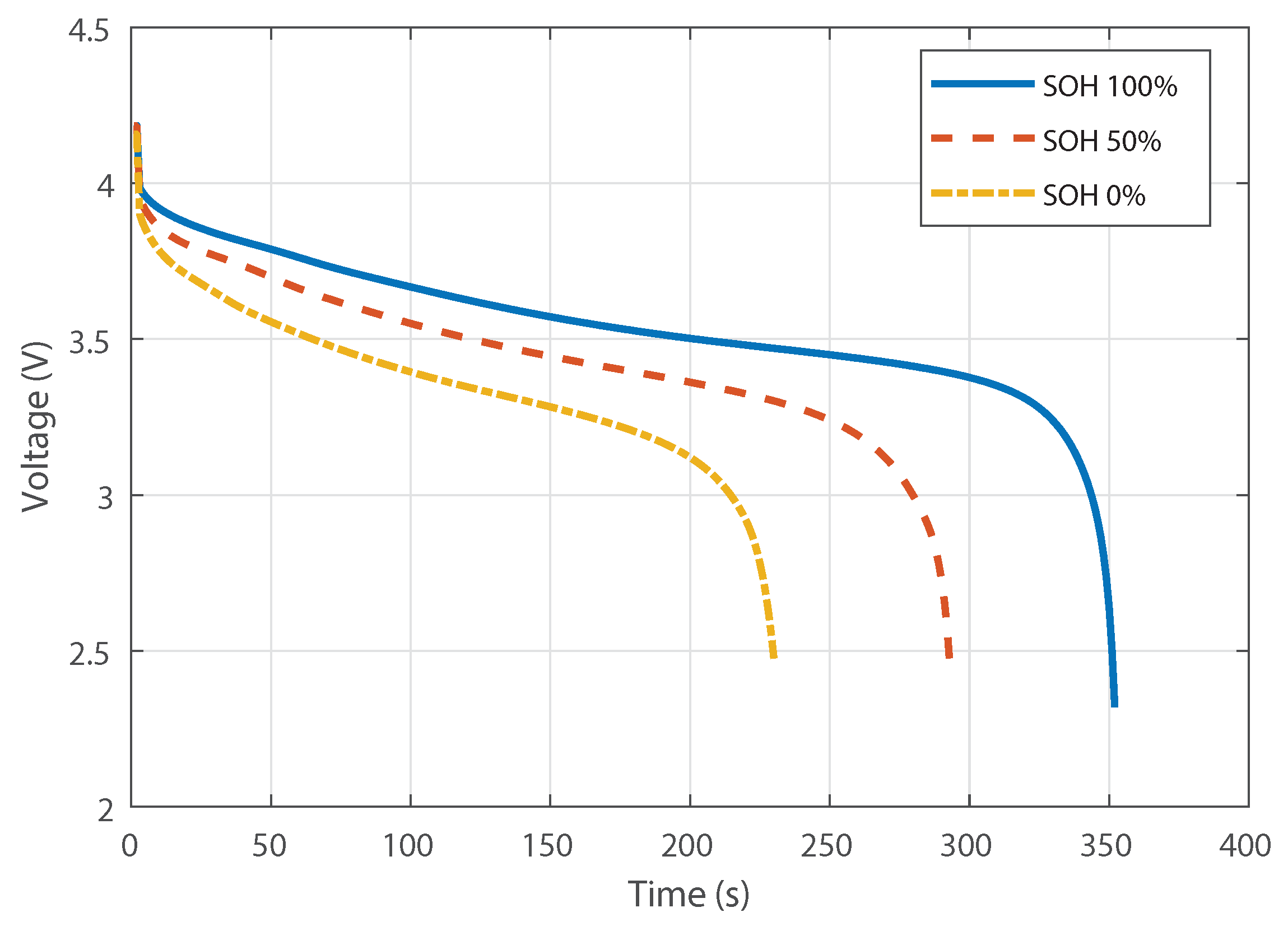
It should be noted that these parameters of the battery are current dependable and can only be observed as the current is drawn from the battery. This curve changes over time for a given current level. Figure 1 shows an example for a current of $2.0$ A.

Since the current drawn provides such an important understanding about the losses inside the batteries, it helps in quantifying the performance of the battery. In literature, the current drawn from the battery is related to the commonly used term C-rate. The C-rate (C/r) is defined as the amount of current drawn in a single discharge cycle of the battery for a given number of hours with respect to its nominal capacity [31]. If a battery has a C-rate of C/10 ($0.1$ A) for a battery of $1.0$ Ah, then this battery will be able to provide charge for 10 h. The amount of energy delivered by a battery and area under the discharge curve also rely on the C-Rate. 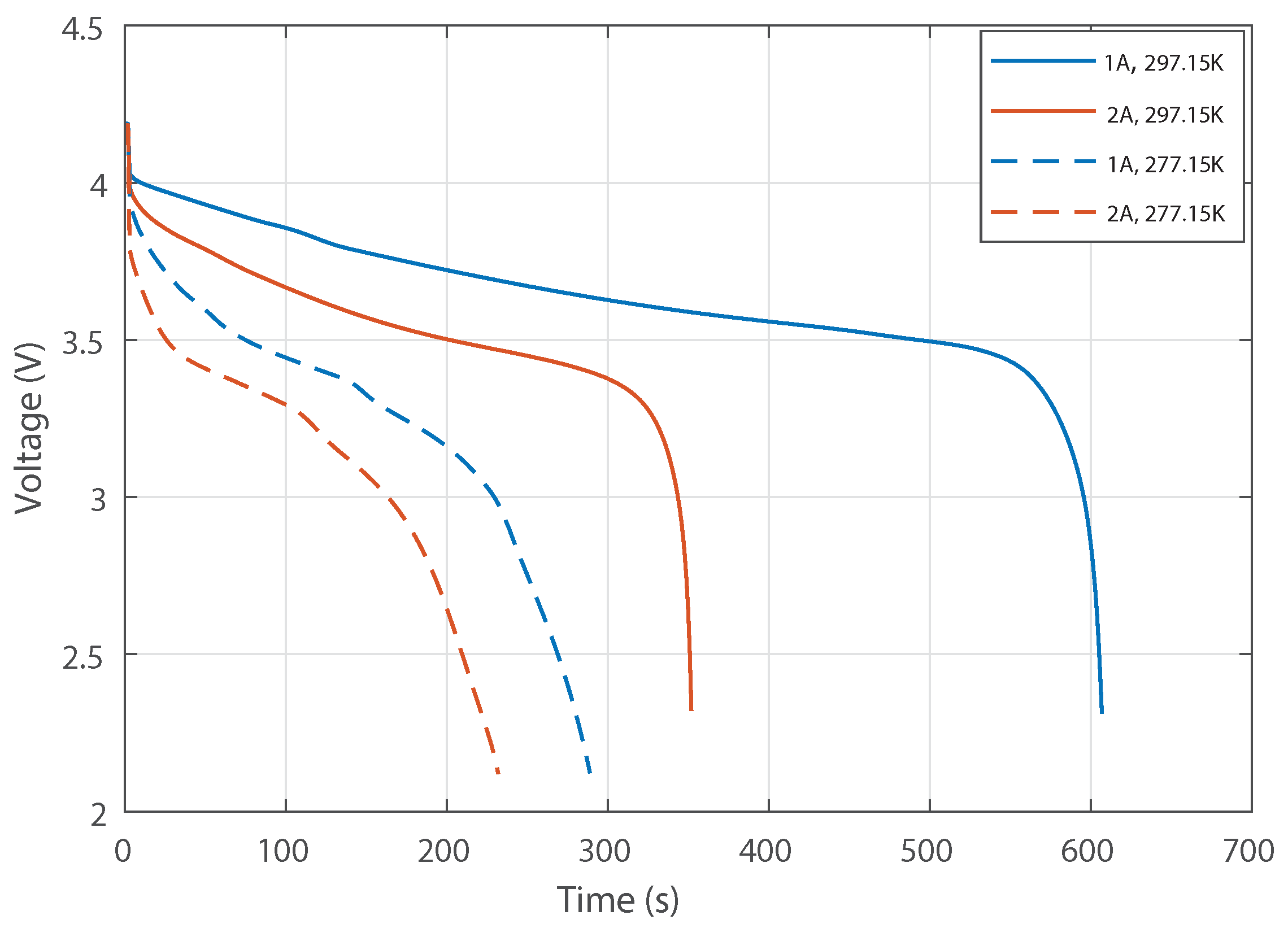Figure 2 shows different current, i.e., $1.0$ A and $2.0$ A, and for different temperatures, i.e., $297.15$ K and $277.15$ K.

There are other parameters which represent the physical properties of batteries, and based on such parameters, different batteries can be used for different applications e.g., grid-scale applications and portable electronic devices. Such parameters include specific energy, specific power, and life cycle. Specific energy is defined as energy per unit weight. Energy stored per unit volume is called energy density. This is an important parameter for the application of portable electronic devices where long-lasting charge is required. Specific power or power per volume is defined as the power density, and is important when sudden charge/discharge is required such as in EVs brakes [32]. Lastly, battery life cycle defines how many charging/discharging cycles a battery can provide before it depletes beyond acceptable limits.

3. Battery Modeling Approach

There are several models that have been used to represent internal characteristics of Li-ion batteries, e.g., black, gray and white box models [2]. The first principal method is categorized as a white-box model; developed with internal battery dynamics such as intercalation kinetics, ion diffusions, and electric potentials. However, the internal electrochemical reactions can be very dull and computationally intractable due to partial-differential equations [33]. Another approach is to use algorithms which are merged with low-order modeling and rely on the slight sacrifice of precision and physical representation [34]. An alternative method is data-driven; it is a model-free approach where machine learning techniques are used. This is a gray/black box model also called the electrical equivalent circuit model [35]. In this model, internal characteristics of a battery are modeled in terms of resistors, capacitors, and inductors. We use the lumped model with approximation of $IR$ drop i.e., the voltage drop caused by electrolyte resistance represented as $R_o$. The activation polarization is denoted as a charge transfer resistance $R_p$ and $C_p$ is the dual layer capacitance in parallel with $R_p$.

Mathematical Model of a Battery

The battery characteristics can be identified using the Randles models [36]. The generalized Randles models have also been used in bio-technologies where a combination of $RC$ and voltage potential is modeled for electrode-tissues interface (ETI) in electroencephalography [37]. In [36], authors have explored the identifiability of Randles models; consisting of [38,39]:

• $R_o$ representing an ohmic resistance due to the conduction of charge carriers through electrolyte and metallic conduction.
• a series of parallel resistor and capacitor connections (i.e., activation polarization) representing the charge transfer resistance and double layer capacitance respectively.

The number of $RC$ parallel circuits defines the order of the circuit model [40].

The electrical behavior of a dual polarization (DP) circuit is represented by following equations [17]:

$$\frac{d{U}_{p1}}{dt}=\frac{I_t}{C_{p1}}-\frac{U_{p1}}{R_{p1}{C}_{p1}}$$

(1)

$$\frac{d{U}_{p2}}{dt}=\frac{I_t}{C_{p2}}-\frac{U_{p2}}{R_{p2}{C}_{p2}}$$

(2)

The output equation in the case of dual polarization (DP) model is given by [17]:

$$y=U_{oc}(SOH)-U_{p1}-U_{p2}-R_o\times I_t,$$

(3)

where $U_{oc}(SOC)$ is the internal voltage of the battery, and $U_{p1}$ and $U_{p2}$ are the voltages across the two $RC$ parallel branches, respectively.

4. Machine Learning for SOH and SOC

Machine learning algorithms are employed here for robust estimation of the battery SOH and SOC. The goal is to calculate the SOH and SOC of a particular battery using a trained regression model, given the battery’s discharge curve and the current voltage-of-operation. The SOH is determined using a machine learning algorithm trained on the discharge curves provided by the NASA Ames prognostic dataset [41], which is shown in

Table 1. Batteries with their current and temperature levels.

S.No	Battery	Current	Temperature
1	B0005	$2.0$ A	$297.15$ K
2	B0006	$2.0$ A	$297.15$ K
3	B0007	$2.0$ A	$297.15$ K
4	B0045	$1.0$ A	$277.15$ K
5	B0046	$1.0$ A	$277.15$ K
6	B0047	$1.0$ A	$277.15$ K

for different current levels (i.e., $1.0$ A, $2.0$ A) and for different temperature levels, (i.e., $297.15$ K and $277.15$ K).

This model looks at a discharge curve of the battery and determines its SOH percentage relative to a reference battery state. This healthy state of the battery is assumed to be the state at the first discharge in the dataset. The SOC at a particular voltage-of-operation $(V_o)$ is determined by utilizing the nature of the discharge curve. The battery has been discharged from a maximum ($V_{max}$) to a minimum ($V_{min}$) voltage. The SOC is estimated by calculating the area under the discharge curve from $V_o$ to $V_{min}$ and dividing this area by the total area under the curve. This provides a quantitative percentage measure of how much charge is left in the battery at a particular voltage-of-operation.

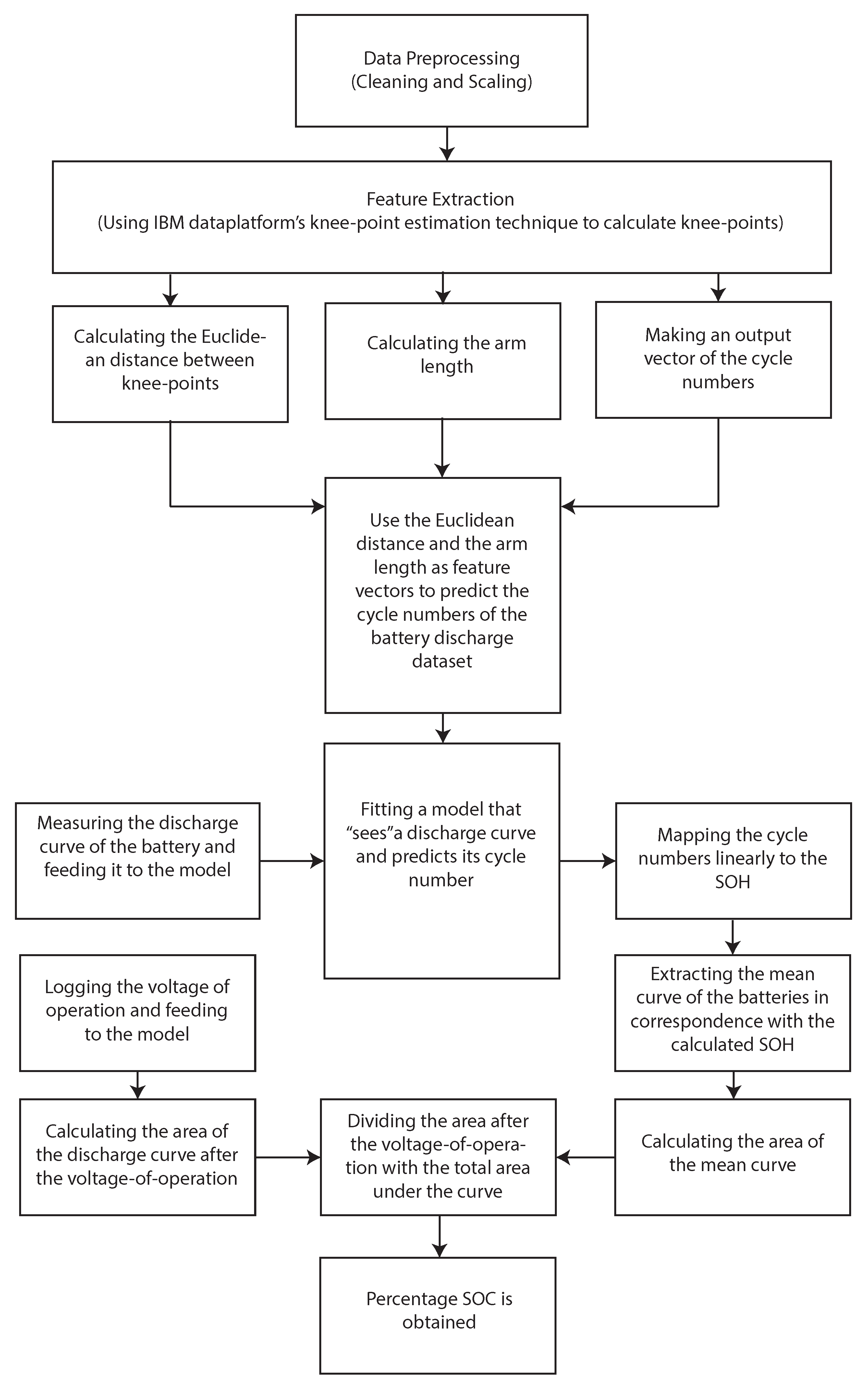
This SOC is then plotted against SOH to get a one-to-one mapping. The end-result is the estimation of SOC given SOH at a specific voltage-of-operation. The following subsection provides more details on the evaluation of SOH and SOC (as shown in block diagram for SOH and SOC Estimation in Figure 3).

4.1. Knee-Point Calculation

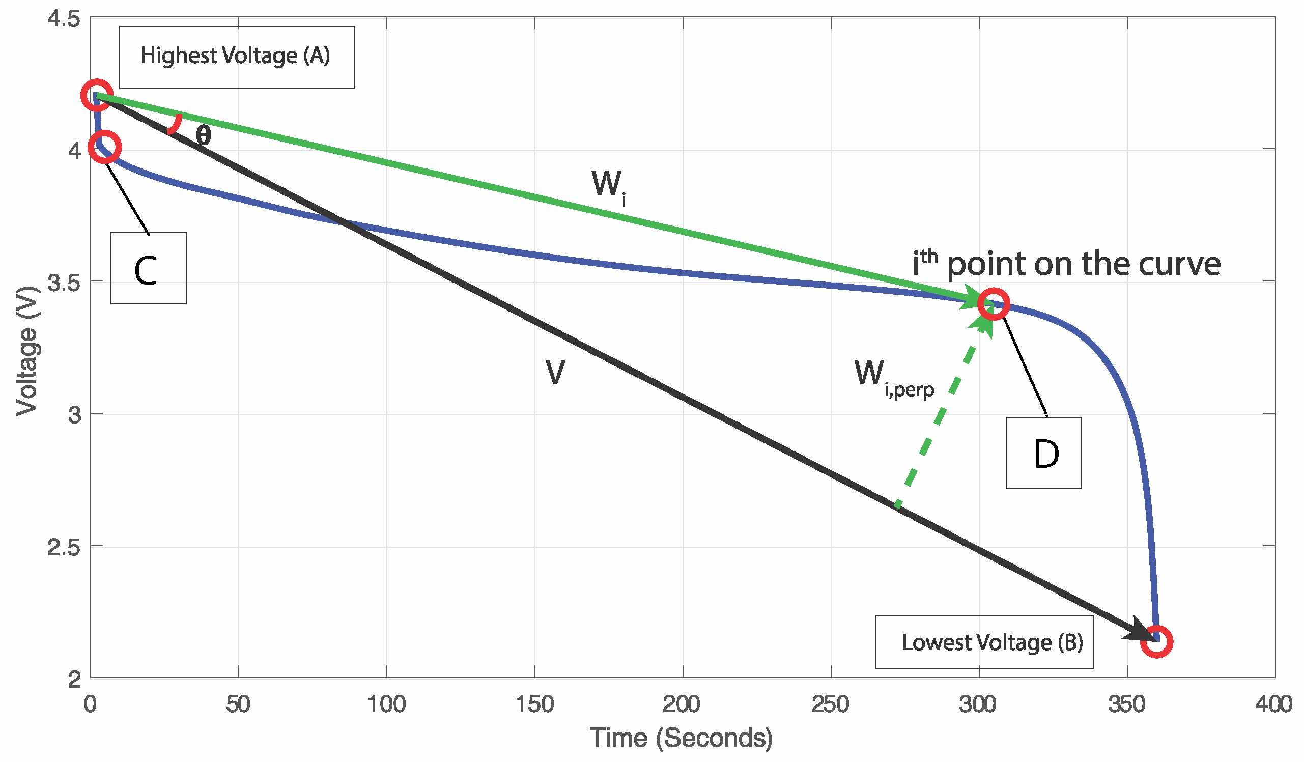
We first convert the discharge voltage vectors into measurable and logical features for SOH estimation. An exemplary discharge curve is shown in Figure 4, where points A and B show the maximum voltage ($V_{max}$) and minimum voltage ($V_{min}$) of the discharge curve, respectively. Points C and D show the two knee-points of the curve. The relative health of the battery decreases with a decrease in the distance between the two knee-points. Hence, the first input parameter becomes the pseudo linear region between the two knee-points of the discharge curve.

An extended version of the algorithm proposed in the IBM data platform [42] is utilized here for the knee point estimation. Specifically, the calculation of the knee points involves two steps; first the equation of the line from the highest voltage $V_{max}$ to the lowest voltage $V_{min}$ of the curve is determined i.e., the straight line passing through points A and B. Then, the largest perpendicular distance from the line $AB$ to the discharge curve is identified. The longest perpendicular distance will represent one of the knee-points of the curve denoted as D. The second knee point C can be determined using a similar approach by applying the algorithm in a region between the start of the curve and the point of intersection between the graph and line $AB$.

To calculate the perpendicular distance from the line to the graph, the dot product is used. Let $AB=V$ and let there be any N points sampled from the discharge curve. Note that the data set already contains N points for each curve of battery discharge. Let $\mathbb{N}=\left\{n_1,\dots ,n_N\right\}$ be the set of all points on the curve such that $<\mathbb{N}>=N$ where $<.>$ denotes the cardinality of the set $\mathbb{N}$. For each $n_i,i\in \{1,2,3\dots ,N\}$, a vector $W_i$ is drawn from point A such that the set of vectors is denoted by $\mathbb{W}=\left\{W_1,\dots ,W_i,\dots ,W_N\right\}$. For each $W_i$, a dot product between V and $W_i$ is taken such that the angle between them is given as:

$${\theta }_i={cos}^{-1}\left(\frac{V·W_i}{\left|V\right|\left|W_i\right|}\right),$$

(4)

where $|.|$ denotes the magnitude operator. The value of the perpendicular distance in terms of the single V, $W_i$ pair is calculated by,

$$W_{i,perp}=W_{i}sin{\theta }_i$$

(5)

The knee-point D, is then found by taking the maxima, i.e.,

$$D={max}_i(W_{1,perp},W_{2,perp},\dots ,W_{N,perp})$$

(6)

For calculating the other knee-point C, the range of the search has to be reduced. This is done by finding the intersection of line $AB$ and the discharge curve, and setting the upper limit of the search equal to the intersection point. Thus, N reduces to a lower value.

4.2. Feature Engineering

An important step in machine learning is the preparation of the dataset to fit our needs. After logging the discharge voltage and time for points A, B, C and D of the battery dataset, the features that would be valuable input parameters in the machine learning model, are extracted. In order to extract these features for the training of the machine learning model, the Euclidean distances $d_{AC}$, $d_{CD}$ and $d_{DB}$ are calculated. Note that the relative health of the battery decreases with a decrease in the distance between the two knee-points. Hence, the first input parameter becomes the Euclidean distance between the two knee-points of the discharge curve (i.e., $d_{CD}$). The line between points C and D is termed the pseudo-linear region due to its linear nature. Now, after determining the first input parameter in the form of the pseudo-linear region, the lengths $AC$ and $DB$ are analyzed as other input parameters to the ML model. The input parameters to the ML algorithm are chosen to be linearly independent to cater for redundancy. The Euclidean distance $d_{CD}$ is identified as a significant feature, therefore other features must be checked if they are linearly independent from the first feature or not. 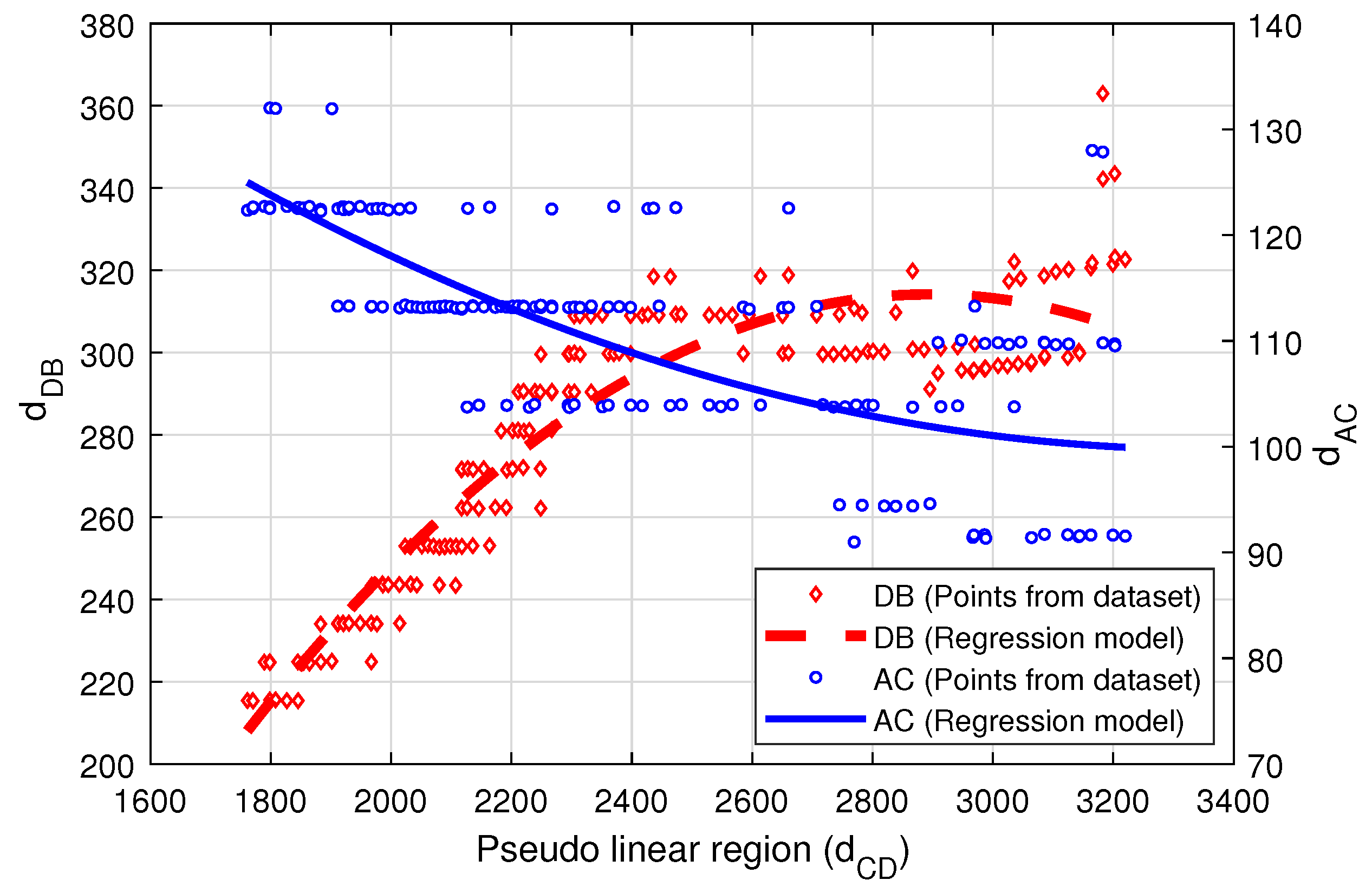Figure 5 represents the relationship between $d_{CD}$ and the other two candidate features such as $d_{AC}$ and $d_{DB}$ for one of the batteries. As $d_{DB}$ provides a more non-linear relationship to $d_{CD}$ than $d_{AC}$, therefore, the second input feature is selected as $d_{BD}$. The length $d_{CD}$ is called as arm length, as it is the length of the offshoot discharge arm of the battery voltage curve.

4.3. Data Preprocessing

The features extracted from each of the discharge curves is used to create the input data matrix, as:

$$\mathit{X}=[{\mathit{x}}_{\mathbf{1}},{\mathit{x}}_{\mathbf{2}}]$$

(7)

where ${\mathit{x}}_{\mathbf{1}}$ and ${\mathit{x}}_{\mathbf{2}}$ are the $(D$ × $1)$ vectors representing the extracted features from the discharge curves if D is the number of discharge curves of a battery. Our dataset contains the discharge curves of a battery in a sequential order. The first discharge curve is assumed to correspond to a healthy battery. After one cycle, the next curve is obtained by charging and discharging this battery again. Hence the nth discharge curve is taken on a battery that has undergone n charges and $(n-1)$ discharges; consequently losing some of its health. We use this characteristic of the dataset to create the output vector of the ML model. The final form of the dataset is:

$$\Delta =[\mathit{X},\mathit{y}],$$

(8)

where each element of $\mathit{y}$ denotes the cycle number corresponding to ${\mathit{x}}_{\mathbf{1}}$, ${\mathit{x}}_{\mathbf{2}}$ features.

4.4. Machine Learning

This dataset is fed into the ML model to determine the best fit. The root mean squared error (RMSE) of each model is calculated to analyze the authenticity and feasibility of the model. It is concluded that a polynomial regression model of 3rd degree provides the best fit with the least RMSE. The hypothesis equation utilized for regression is given below:

$$h_{\theta }(x_1,x_2)={\theta }_0+{\theta }_1{x}_1+{\theta }_2{x}_2+{\theta }_3{x}_1^2+{\theta }_4{x}_1{x}_2+{\theta }_5{x}_1^3+{\theta }_6{x}_1^2{x}_2$$

(9)

The values of the parameters are determined by using the gradient descent algorithm. This algorithm quantitatively compares the predicted value of cycle number from the model to the ground truth $\mathit{y}$ of the dataset. The following equation calculates the RMSE of the ML model;

$$J(\theta )=J({\theta }_0,\dots ,{\theta }_6)=\frac{1}{2m}{\mathsf{\Sigma }}_{i=1}^m{(h_{\theta }(x_1^{(i)},x_2^{(i)})-{\mathit{y}}_{\mathit{m}})}^2,$$

(10)

where J is the cost or error function quantifying the RMSE of the model, m is the size of the dataset and $\theta$ is the vector containing the model parameters ${\theta }_0,\dots ,{\theta }_6$. To minimize this error, we must tweak the model parameters and find the optimum values recursively. To get the new values of the model parameters ${\theta }_{n+1}$, we take the partial derivatives of the error term with respect to each of the parameters in vector ${\theta }_n$ and subtract this derivative term from ${\theta }_n$.

$${\theta }_{n+1}:={\theta }_n-\alpha \frac{\partial }{\partial {\theta }_n}J({\theta }_0,\dots ,{\theta }_6)$$

(11)

This process is then repeated with the new parameter values to minimize the error function and push it closer to zero. An ideal cost function will have a value of 0.

The first discharge cycle will correspond to a battery health of 100% and the last discharge cycle will provide the discharge curve of the least “healthy” battery.

4.5. SOC Estimation

The ML model uses the entire discharge curve to estimate the SOH of the battery. Now the current voltage-of-operation is provided as another parameter to the algorithm. The goal is to provide an estimated amount of charge, that is left in the battery at a certain voltage-of-operation $(V_a)$. To do so, the curve from the maximum $V_o$ to the minimum $V_{min}$ is used. As provided in the NASA Ames prognostic repository, the battery has been discharged till $+2.7$ V. Hence, only part of the curve up to that point will be used.

After extracting the voltage curve from $V_{max}$ to $+2.7$ V, the area $A_T$ under the curve is calculated. Now, the given voltage $V_o$, which is the current voltage-of-operation of the battery, is used. The total charge remaining in a battery of a specific SOH, at a particular $V_o$ is calculated by dividing the area under the curve after $V_o$ to $+2.7$ V, by the total area of the curve. This gives an estimate of the percentage of charge left in the battery at a particular voltage level. The formula for $SOC\%$ calculation is given by:

$$SOC\%=\frac{{\int }_{V_o}^{+2.7V}V(t)dt}{A_T},$$

(12)

where $V(t)$ is the discharge curve function with respect to time and the nominator term represents the area from $V_o$ to $+2.7$ V.

5. Results and Discussions

In this section, the method is implemented on six batteries with different current and temperature levels. The first three batteries are modeled with a current level of $1.0$ A and a temperature of $297.15$ K. Similarly, the other three batteries are modeled with a current level of $2.0$ A and a temperature of $277.15$ K. Note that each battery has different cycles, therefore, each battery represents a different trend when plotted against the pseudo-linear region $(d_{CD})$ and arm length $(d_{DB})$.

The discharge curve labeling has been implemented by knee point calculation. This step accurately specifies the threshold voltages for feature estimation. $d_{CD}$ and $d_{DB}$ are extracted as features since $d_{CD}$ represents the capacity of the battery and $d_{DB}$ provides remaining 10% of charge with EOD point. This not only helps in finding the SOH, but also the SOC at any instance of time. Moreover, this algorithm could have also estimated SOH of batteries at higher temperature and load current levels, given a larger dataset. Nevertheless, implementing the proposed algorithm using $277.15$ K and $297.15$ K temperature and $1.0$ A and $2.0$ A current levels, respectively are sufficient verification of this method.

The datasets of batteries are divided into two major portions; training and testing. Such classification of data is important to verify the performance of the developed models. In doing so, our classification is purely done randomly i.e., out of all the discharge curves, 70% of them are randomly chosen for training and remaining 30% of the discharge curves are dedicated to the testing of the model.

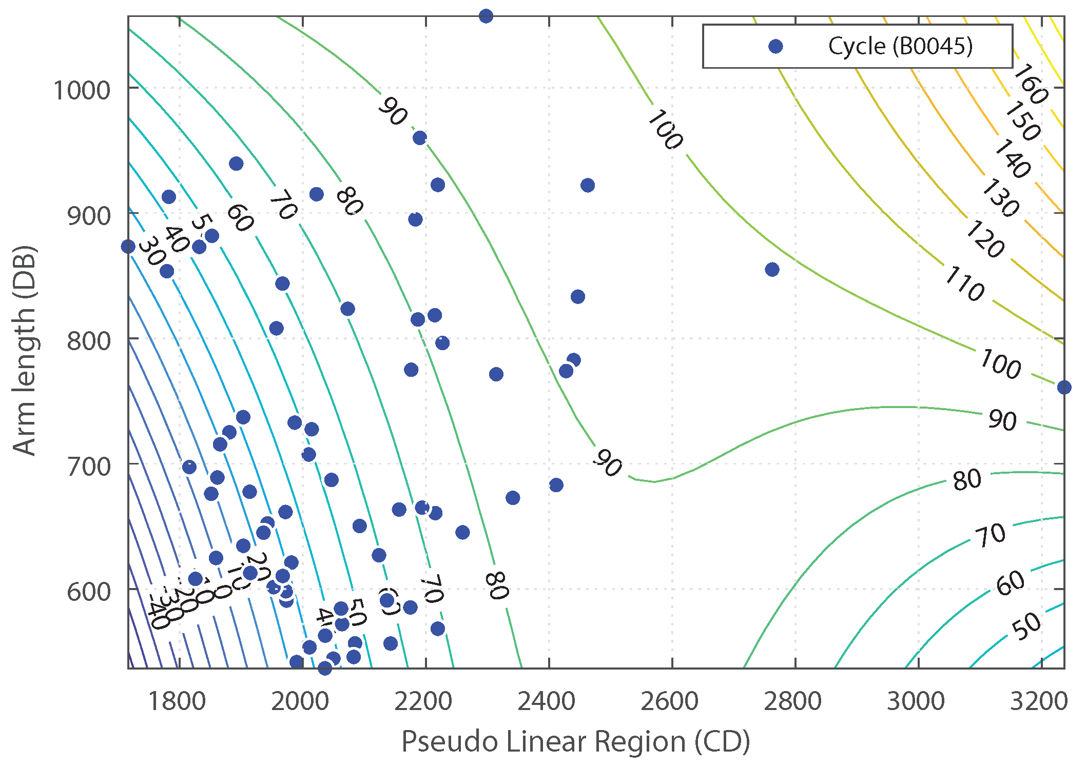
First, the results showing the relationship between the two extracted features of a battery curve versus the cycle number or SOH are presented. Note that the dataset contains the cycle number of each discharge curve, whereas the battery health is generally taken in terms of SOH. Therefore, a mapping between cycle number and SOH is performed, such that the greater the cycle number the lesser the SOH.

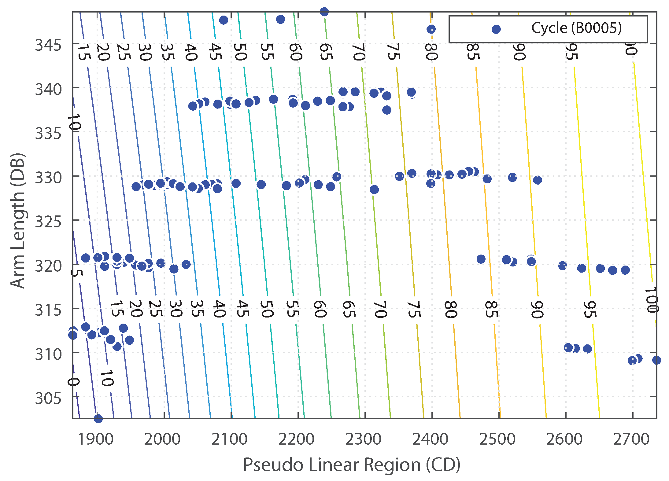
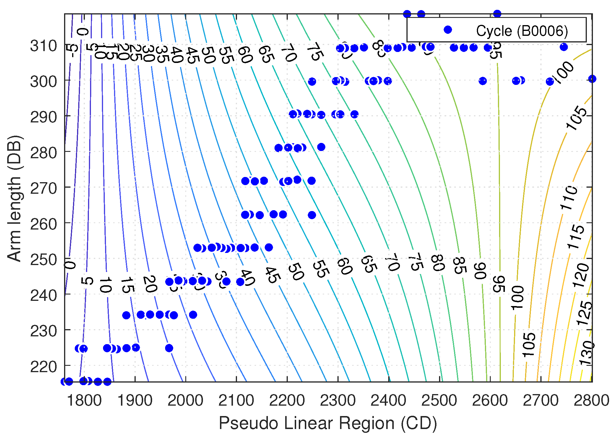
Figure 6, Figure 7 and Figure 8 represent the contour plots of the models used for the estimation of the SOH of the batteries at $297.15$ K. The training dataset used in each case is shown by points on the graph. It can be inferred from the graph that with the increase in the $d_{CD}$ and $d_{DB}$ the SOH also increases. It should be noted that the SOH is given in the form of a percentage metric but the contour lines go above 100% on the right side of the contour plots. The reason behind this apparent anomaly is that the ML model predicts the SOH without any regard to the nature of the SOH. Thus, no input features are ever provided that take the SOH above 100%. For this model, SOH is just a numeric value though there are no “real” data points in the above 100% region. 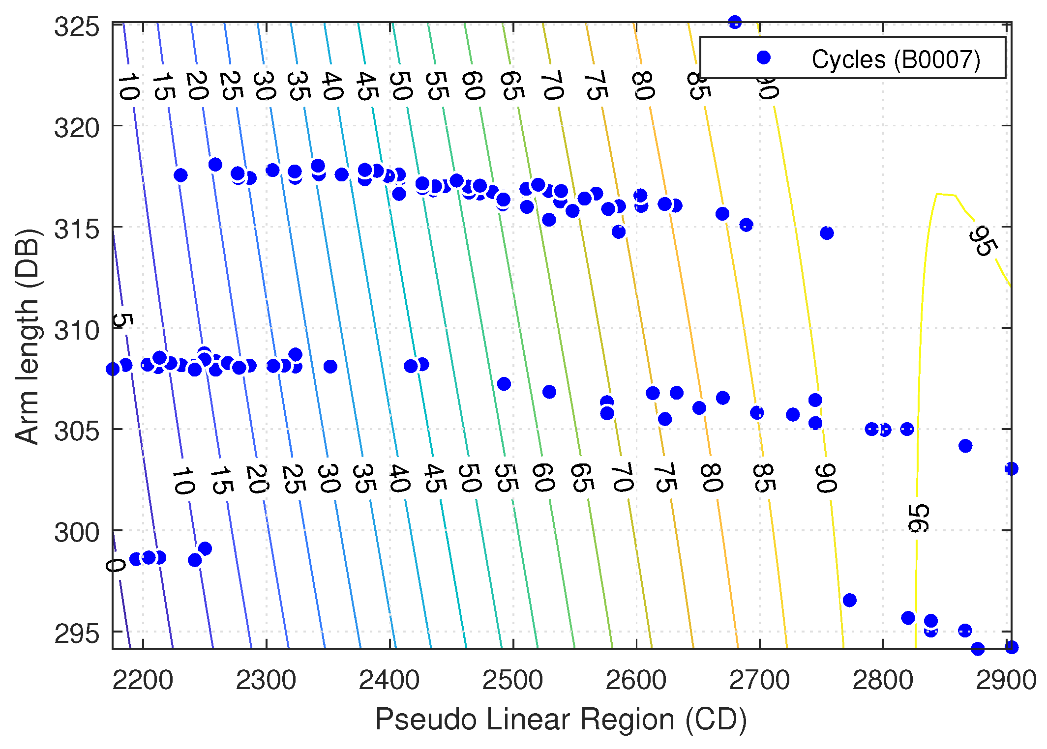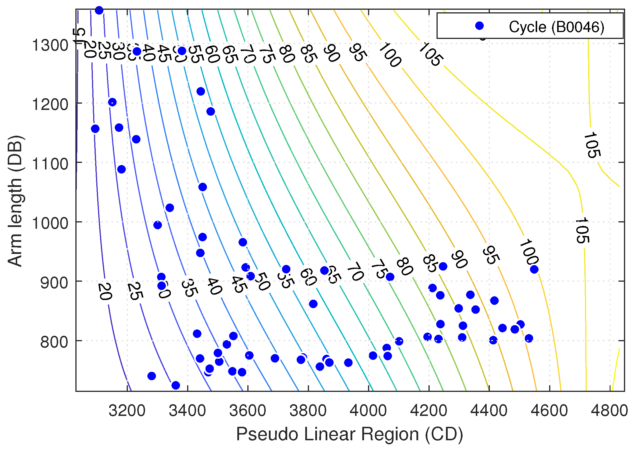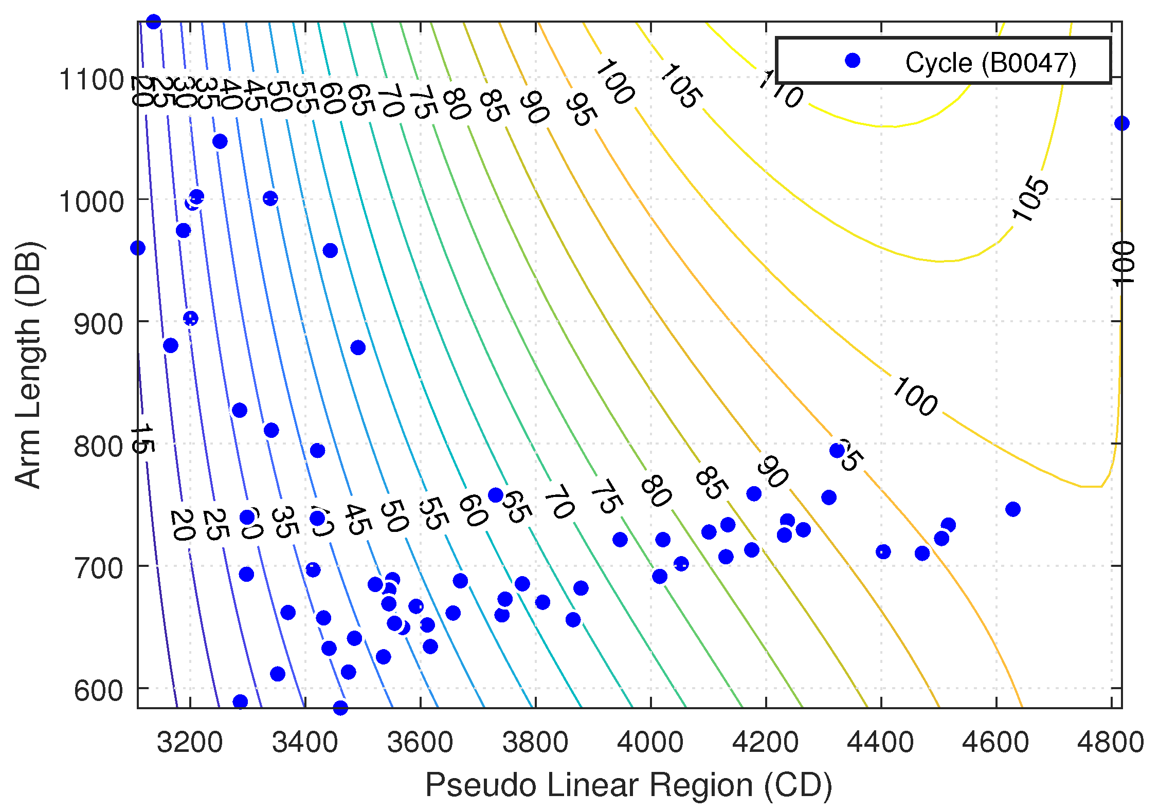Similarly, Figure 9, Figure 10 and Figure 11 show contour plots of the models estimating the SOH at $277.15$ K. Note that, in the contour plot of each of the battery, the blue circles show the cycles, whereas the lines correspond to SOH. Similarly, if these points are connected together a 3rd polynomial trend can be obtained as represented by Equation (9).

The increase in the SOH of the battery causes the overall area of the voltage curve to increase. This increased area is in the denominator of the term that calculates the percentage SOC and henceforth, decreases the SOC. This percentage decreases much more rapidly as compared to a healthy battery because of its reduced capacity. Thus, it can be concluded, for a particular value of the voltage, the SOC of the battery increases with the decrease in health, i.e., the battery loses charge faster when it has a low SOH. The overall curve is uneven and has higher peaks at the ends. The main reason for such abnormality is due to the sparsity of the dataset. The inclusion of such result may depict rough estimation. However, it is very important to draw a relationship between SOH and SOC together for a particular voltage, which not only broadens the understanding of these two parameters but also introduces a correlation between them.

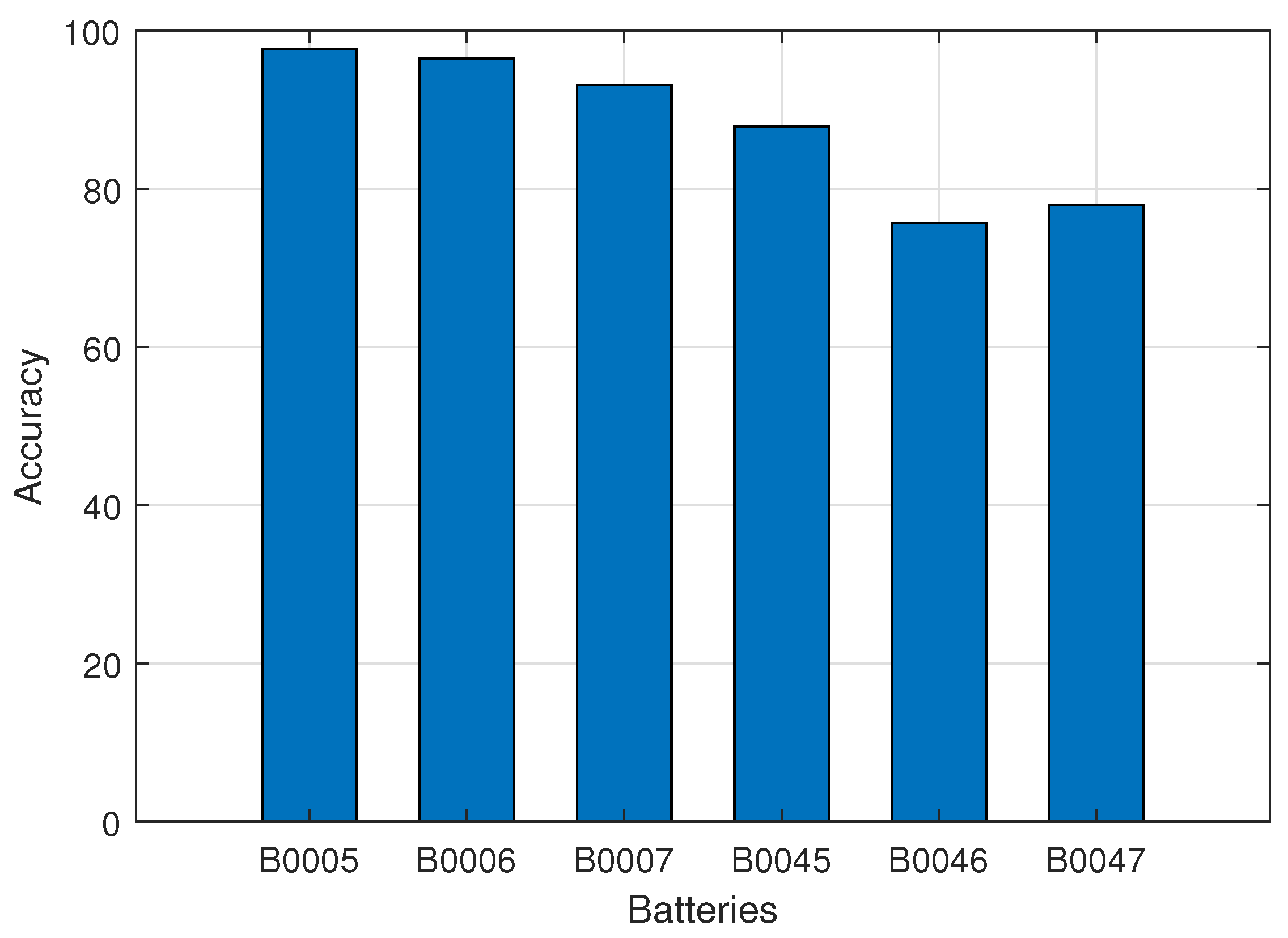
Finally, it is worthwhile noting that the accuracy of the three batteries (B0045-B0047) with a temperature of $277.15$ K and a current of $2.0$ A, has lower values (87.86% to 77.87%) in comparison to that of $297.15$ K and $1.0$ A batteries (93.08% to 98.00%). This is mainly due to the small size of datasets and larger gaps between adjacent discharge curves, which increase the error between training versus testing results. Such an error can be minimized with larger and more precise datasets. The accuracy shown in Figure 12 is calculated by:

$$Accuracy=100-\frac{1}{N}\left[\sum _{i=1}^{N_{test}}\frac{{\widehat{SOH}}_i-SO{H}_i^{(t)}}{SO{H}_i^{(t)}}\right]\times 100$$

(13)

where, $N_{test}$ is the number of discharge cycles of the test dataset, ${\widehat{SOH}}_i$ is the $i_{th}$ term of estimated SOH, and $SO{H}_i^{(t)}$ is the $i_{th}$ true value of discharge curve driven by the training dataset.

6. Conclusions

This work summarized some of the important contributions for battery management systems (BMS). In an initial stage of this research, important findings are made in the estimation of SOH and SOC using the ML approach. As the behavior of the battery is non-linear and cannot be predicted directly, therefore, an indirect estimation and prediction method is needed. In the estimation of battery SOH and SOC, several features were extracted from discharge curves of different batteries with current and temperature levels, i.e., B0006 is a battery with $2.0$ A and $297.15$ K, whereas, B0047 is a battery with $1.0$ A and $277.15$ K. During the extraction of features, a knee-point calculation technique was implemented, which identified knee-points numerically. The calculated features are fed to the ML model, which provide SOH over all discharge cycles of the battery with respect to the pseudo-linear region and arm length. In addition, the SOC% was estimated by considering the area under the curve of the measured voltage. This technique has not only estimated the correct SOC% for a discharge cycle, but has also provided a decreasing trend with respect to all training cycles. In other words, if we are given a battery at any instant of time, we can estimate its SOC by considering its voltage as a reference point and using reverse engineering to calculate the SOH.

However, due to a limited dataset, the obtained error was significant, which can be minimized in with the use of larger datasets. Despite the fact that the Polynomial regression models stand out over other ML techniques as they provide the best RMSE, this might not be possible with large datasets. Therefore, better methods such as ANN and support vector machines can be implemented in the future. Finally, since the proposed model needs the entire discharge curve to calculate the SOH and SOC of the battery, and with a larger dataset, recurrent neural networks might be a better choice for online estimation of SOH.