A New Generalized Morse Potential Function for Calculating Cohesive Energy of Nanoparticles

Abstract

A new generalized Morse potential function with an additional parameter m is proposed to calculate the cohesive energy of nanoparticles. The calculations showed that a generalized Morse potential function using different values for the m and α parameters can be used to predict experimental values for the cohesive energy of nanoparticles. Moreover, the enlargement of the attractive force in the generalized potential function plays an important role in describing the stability of the nanoparticles rather than the softening of the repulsive interaction in the cases when m > 1.

1. Introduction

Cohesive energy is an important quantity that is used to drive almost all the thermodynamical properties of materials [1] and is defined as the energy needed to dissociate a solid to its neutral atomic components [2]. Cohesive energy can be calculated by summing the total potential energies of all atoms in the solid materials. Many theoretical models were developed to investigate the size-dependent cohesive energy such as bond energy model [3,4], surface-area-difference model [1], embedded-atom-method potential [5], thermodynamic model [6,7], and a nonlinear, lattice type-sensitive model [8,9]. Other models were also proposed to calculate the cohesive energy based on the potential energy functions between two atoms inside metallic nanoparticles such as the Lennard–Jones (or L–J (12-6)) potential function [10,11], the Mie-type $\left(m,n\right)$ potential function [12], and the Morse potential function [13]. Predicting cohesive energies and stabilities in solid particles can be enhanced by re-parameterization (the bond order parameters) of the analytic potential functions such as: A force field for zeolitic imidazolate framework-8 (ZIF-8) with structural flexibility [14], parameterized analytical bond order potential for ternary the Cd–Zn–Te systems [15].

Potential energy functions contain a certain number of parameters. For example, the Mie-type potential function contains two parameters $\left(m,n\right)$ (where $m>n$) [16]. The Morse potential function contains one parameter, $\alpha$ [17]. These parameters determine the strength and the range of the interaction terms in the potential functions. The L–J potential function consists of two terms: The first term represents Pauli’s repulsion, whereas the second term represents the attractive dipole [2].

Qi et al. [10] found a disagreement between the calculated cohesive energies arising from the L–J (12-6) potential function and the experimental values of molybdenum (Mo) and tungsten (W) nanoparticles in a face-centered cubic structure. However, the calculated cohesive energies using the L–J (12-6) potential function agreed with the experimental values of Mo and W nanoparticles in a regular octahedron structure [11]. Moreover, there was an agreement between the experimental values for the cohesive energy of Mo and W nanoparticles and the calculated cohesive energy using the Mie-type $\left(m,n\right)$ potential function (with $m=6$ and $n=5$) [12] and the Morse potential function (with $\alpha \approx 3$) [13]. The stability of nanoparticles using the Mie-type potential function $\left(6,5\right)$ and the Morse potential function ($\alpha \approx 3$) was found to be a result of the softening in the repulsive interaction [12,13] in the potential functions. However, the interaction terms in the Mie-type potential function $\left(6,5\right)$ and the Morse potential function ($\alpha \approx 3$) do not represent the Pauli repulsion and attractive dipole terms.

A modified Morse/long-range potential function was proposed to analyze the spectroscopic data of diatomic molecules N₂ [18] and Co₂-H₂ complexes [19]. The aim of the present work was to propose a new generalized Morse potential function that can predict the experimental values of cohesive energy of nanoparticles. The proposed potential function should contain a term that represents the Pauli repulsion interaction [2].

The paper is organized as follows. In Section 2 we describe the generalized Morse potential theory. In Section 3, we describe a model to calculate the cohesive energy for nanoparticles based on the generalized Morse potential. Finally, in Section 4, we discuss the numerical results with present conclusions.

2. Theory

The potential energy $U_{ij}$ that describes the bond between two atoms $i$ and $j$ in the nanoparticle separated by a distance $r_{ij}$ has a complicated form which can be written in series form as:

$$U_{ij}\left(r_{ij}\right)=U_{ij}\left(r_0\right)+{\frac{d{U}_{ij}}{d{r}_{ij}}|}_{r_0}\left(r_{ij}-r_0\right)+{\frac{d^2{U}_{ij}}{d{r}_{ij}{}^2}|}_{r_0}{\left(r_{ij}-r_0\right)}^2+{\frac{d^3{U}_{ij}}{d{r}_{ij}{}^3}|}_{r_0}{\left(r_{ij}-r_0\right)}^3+\cdots ,$$

(1)

where $r_0$ is the distance between the nearest two atoms in equilibrium case. The potential energy that describes the bond between the two atoms should satisfy the following requirements: (1) The potential should have one minimum point $-D$ at $r_{ij}=r_0,$ (2) it should asymptotically go to zero as $r_{ij}\to \infty$, and (3) it should become infinite at $r_{ij}=0$.

A well-known potential that satisfies the requirements is the Morse potential [17]:

$$U_{Mij}=D\left(e^{-2\alpha \left(\frac{r_{ij}}{r_0}-1\right)}-2e^{-\alpha \left(\frac{r_{ij}}{r_0}-1\right)}\right),$$

(2)

where $\alpha$ is a unitless parameter depending on type and structure of metallic nanoparticles [20]. Lim [21,22] found that the parameter $a$ can be expressed in terms of the Lennard–Jones parameters.

The Morse potential function contains two terms: The first term represents the attractive short-range interaction, whereas the second term represents the repulsive long-range interaction. However, the Morse potential function can be written using a summation form as follows:

$$U_{Mij}=D{\displaystyle \sum _{k=1}^2}{\left(-1\right)}^k\left(2-\left(k-1\right)\right)e^{-k\alpha \left(\frac{r_{ij}}{r_0}-1\right)}.$$

(3)

The Morse potential function is the simplest form that was proposed to describe the interaction potential between two atoms in metallic nanoparticles [13]. The form of the interaction potential function between two atoms in metallic nanoparticles is more complex than the Morse potential, the Morse potential was formulated by considering only the first three terms of the series in Equation (1) [17]. However, if more terms are considered, then additional exponential terms of higher order emerge.

In this current work, a new generalized Morse potential function was proposed that includes more than two interaction terms. The additional terms are controlled by a new unitless parameter $m$ ($=1,2,3,\cdots$) as follows:

$$U_{GMij}=\frac{D}{m}{\sum }_{k=1}^{2m}{\left(-1\right)}^k\left(2m-\left(k-1\right)\right)e^{-k\alpha \left(\frac{r_{ij}}{r_0}-1\right)}.$$

(4)

For example, if $m=3$, then the generalized Morse potential function will contain six terms. If $m=1$, then the generalized Morse potential function becomes the ordinary Morse potential function.

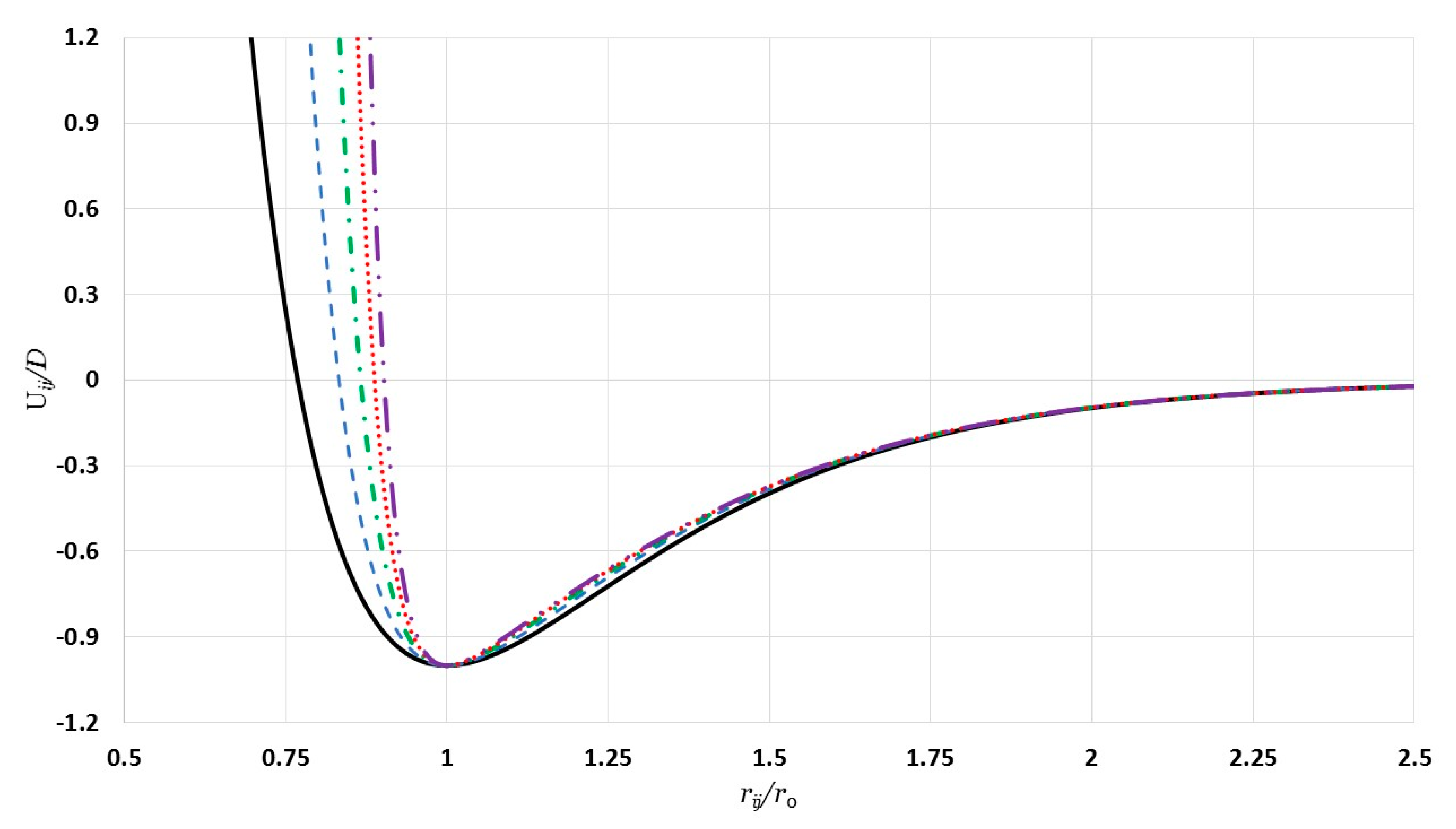
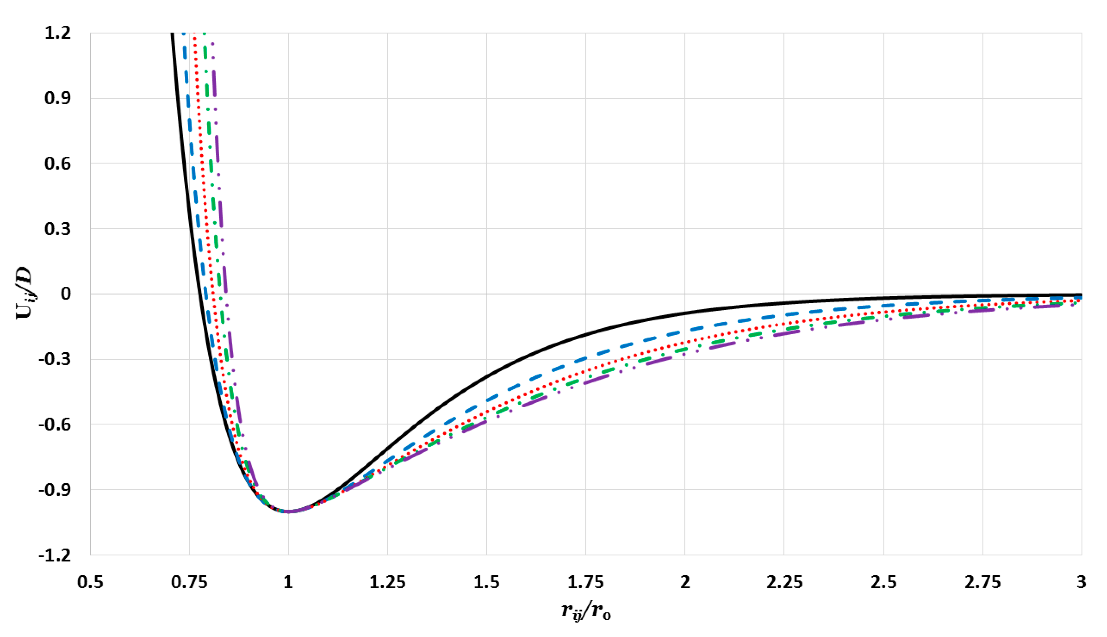
The curves in Figure 1 represent the generalized Morse potential as a function of reduced separated distance between two atoms for a fixed value of $\alpha$ and different values of $m$. All potential curves in Figure 1 satisfy all requirements of the potential energy between the two nearest atoms in a nanoparticle. As seen in Figure 1, when $m>1$ the repulsive wall becomes stiffer with little change in the range of the attractive interaction. Moreover, the repulsive walls of the potential curves converge as $m$ and they become large, as seen, again, in Figure 1.

3. The Model

The cohesive energy of the nanoparticles is obtained by the summation of the total energy of $n$ atoms in a nanoparticle:

$$E_n=\frac{nD}{2m}{\sum }_{k=1}^{2m}{\left(-1\right)}^k\left(2m-\left(k-1\right)\right)A_k\left(r^{*}\right),$$

(5)

where

$$A_k\left(r^{*}\right)=\frac{1}{n}{\sum }_{i=1}^n{\sum }_{\begin{array}{c}j=1\\ i\ne j\end{array}}^n{e}^{-\alpha k\left(a_{ij}{r}^{*}-1\right)},$$

(6)

$a_{ij}=r_{ij}/r$ ($r$ is the nearest distance between two atoms) and $r^{*}=r/r_0$ is the reduced nearest distance between two atoms. Moreover, $A_k\left(r^{*}\right)$’s ($k=1,2,\cdots ,2m$) in Equation (6) represents the interaction terms of the potential. The range of the interaction terms varies from the shortest range ($k=2m$) to the longest range ($k=1$).

The cohesive energy of the nanoparticle is calculated in an equilibrium configuration for $n$ atoms. The equilibrium configuration is obtained by minimizing the total energy of $n$ atoms in the nanoparticle with respect to $r^{*}$ $\left({\frac{d{E}_n}{d{r}^{*}}|}_{r^{*}=r_0^{*}}=0\right)$, where $r_0^{*}$ is the equilibrium reduced nearest distance between two atoms, which is obtained numerically.

The cohesive energy per atom in the equilibrium configuration is:

$$E_a=\frac{D}{2m}{\displaystyle \sum _{k=1}^{2m}}{\left(-1\right)}^k\left(2m-\left(k-1\right)\right)A_k\left(r_0^{*}\right).$$

(7)

The relative cohesive energy of the nanoparticle is the ratio between the cohesive energy per atom and the cohesive energy of the corresponding bulk material $E_0$:

$$\frac{E_a}{E_0}=\frac{P_0}{2m}{\displaystyle \sum _{k=1}^{2m}}{\left(-1\right)}^k\left(2m-\left(k-1\right)\right)A_k\left(r_0^{*}\right),$$

(8)

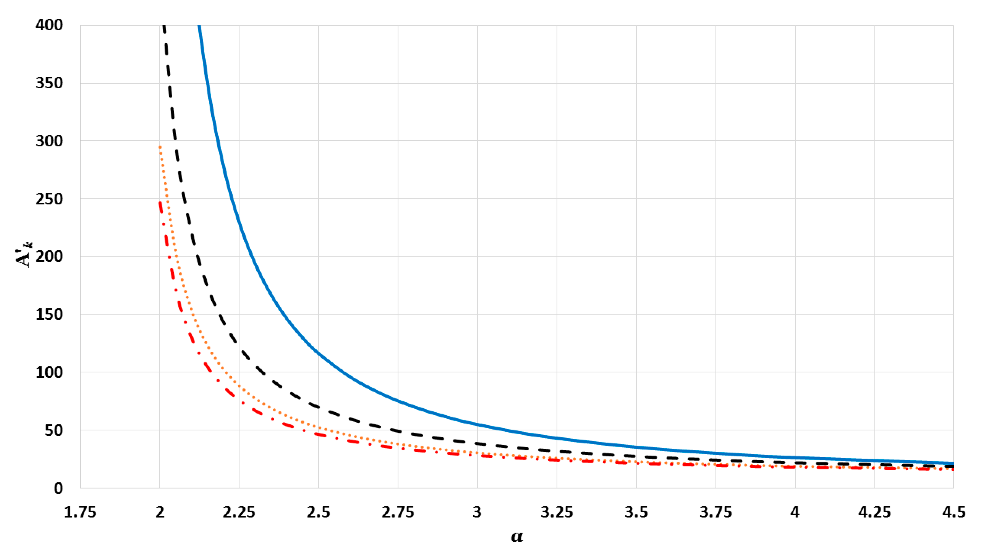
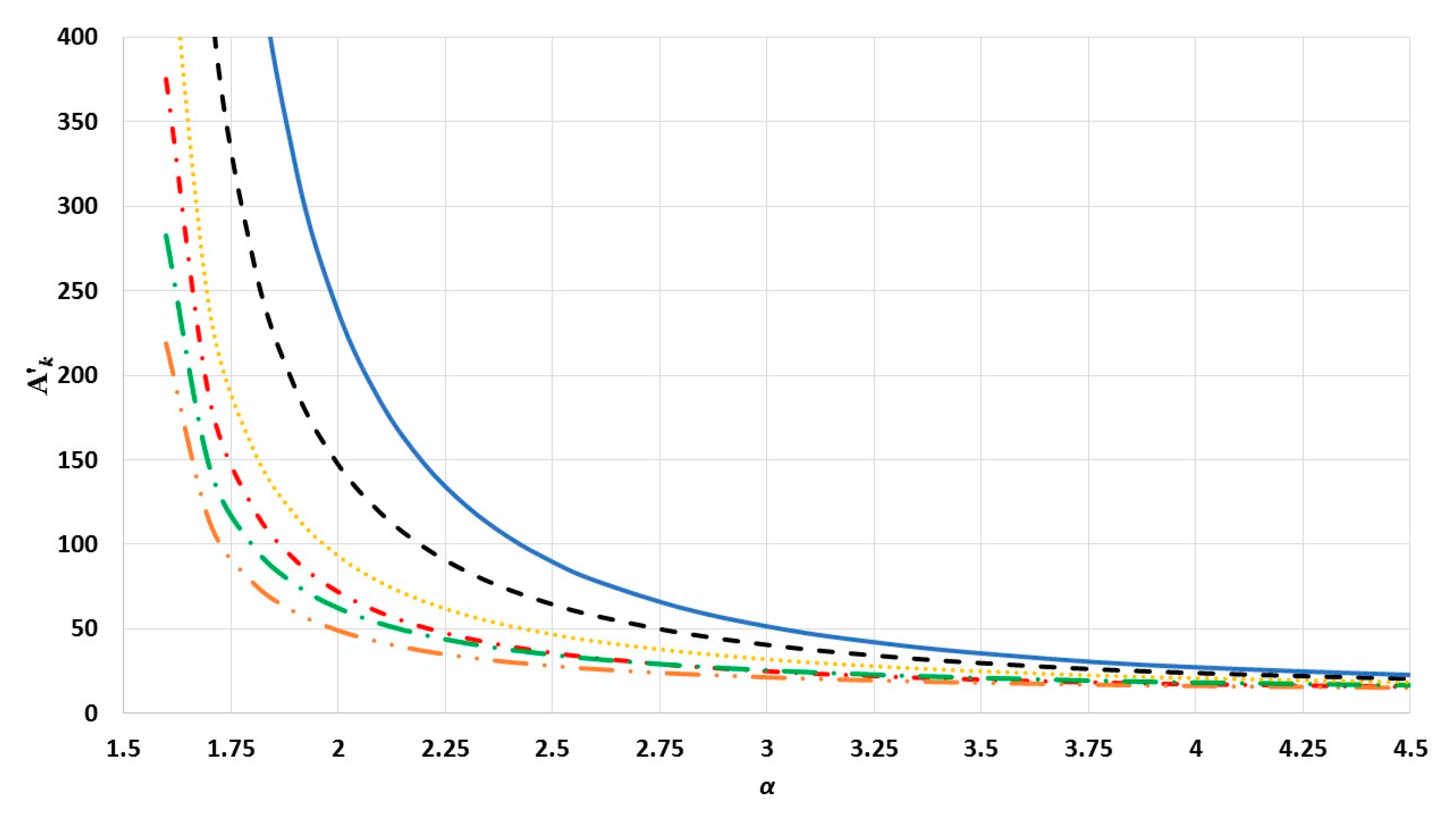
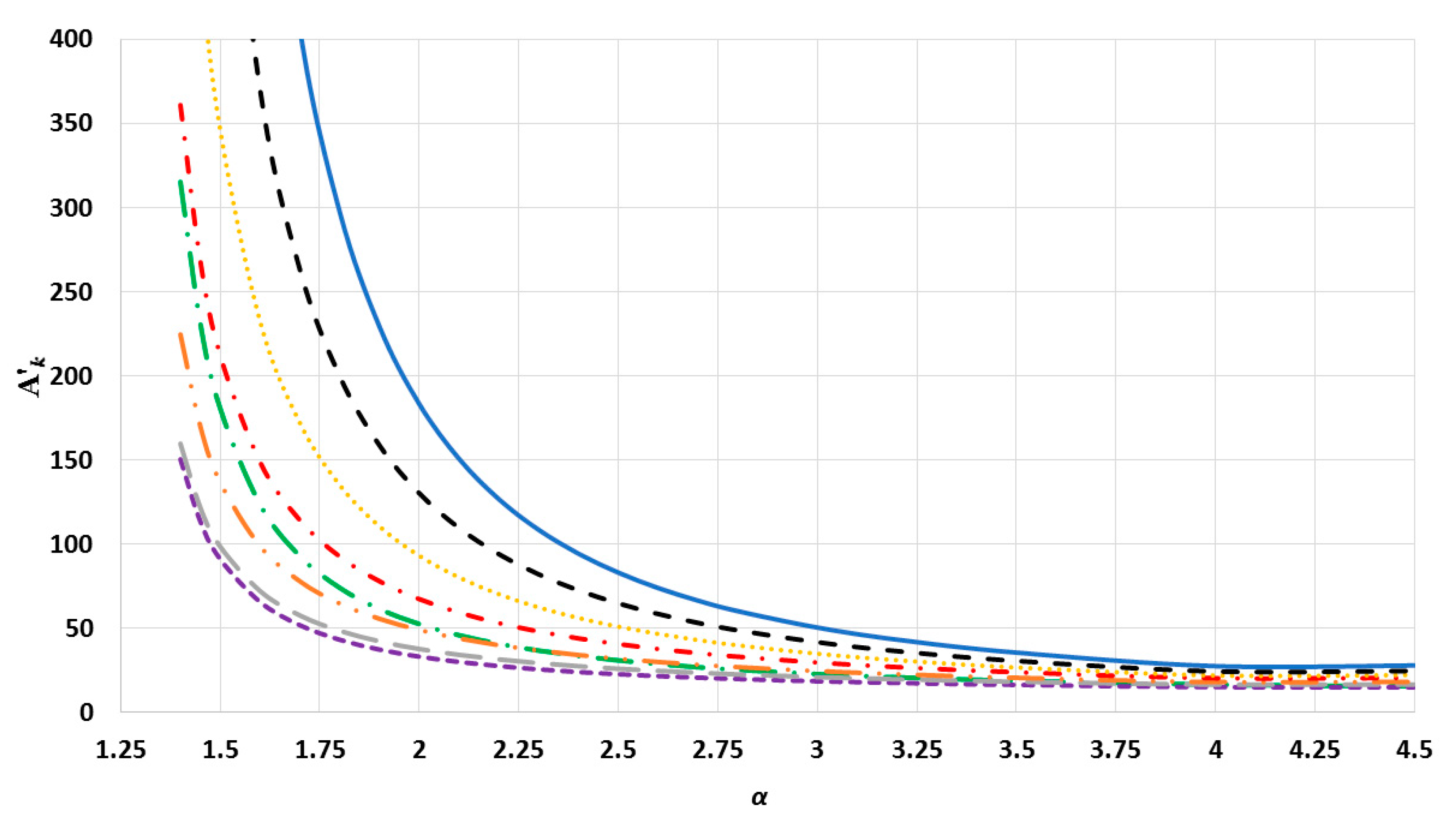
where $P_0=2m/[{\sum }_{k=1}^{2m}{(-1)}^k(2m-(k-1)){A^{\prime }}_k(r_0^{*})]$ and ${A^{\prime }}_k\left(r_0^{*}\right)$’s are the corresponding interaction terms of bulk metals (as $n\to \infty$). The values of interaction terms ${A^{\prime }}_k\left(r_0^{*}\right)$’s for given $m$ vary with the $\alpha$ parameter, as seen in Figure 2, Figure 3 and Figure 4. The values of interaction terms ${A^{\prime }}_k\left(r_0^{*}\right)$’s grow rapidly to infinity as the value of $\alpha$ parameter decreases. Nevertheless, as this is not physically acceptable, a valid range for the $\alpha$ parameter is defined, such that the values of ${A^{\prime }}_k\left(r_0^{*}\right)$’s are finite. It was thus found that for different cubic metallic structures, the valid range for the $\alpha$ parameter is approximately the same when $m=1$ [13]. Therefore, the values of the interaction terms ${A^{\prime }}_k\left(r_0^{*}\right)$ in Figure 2, Figure 3 and Figure 4 are only for a face-centered cubic metallic structure.

4. Results and Discussion

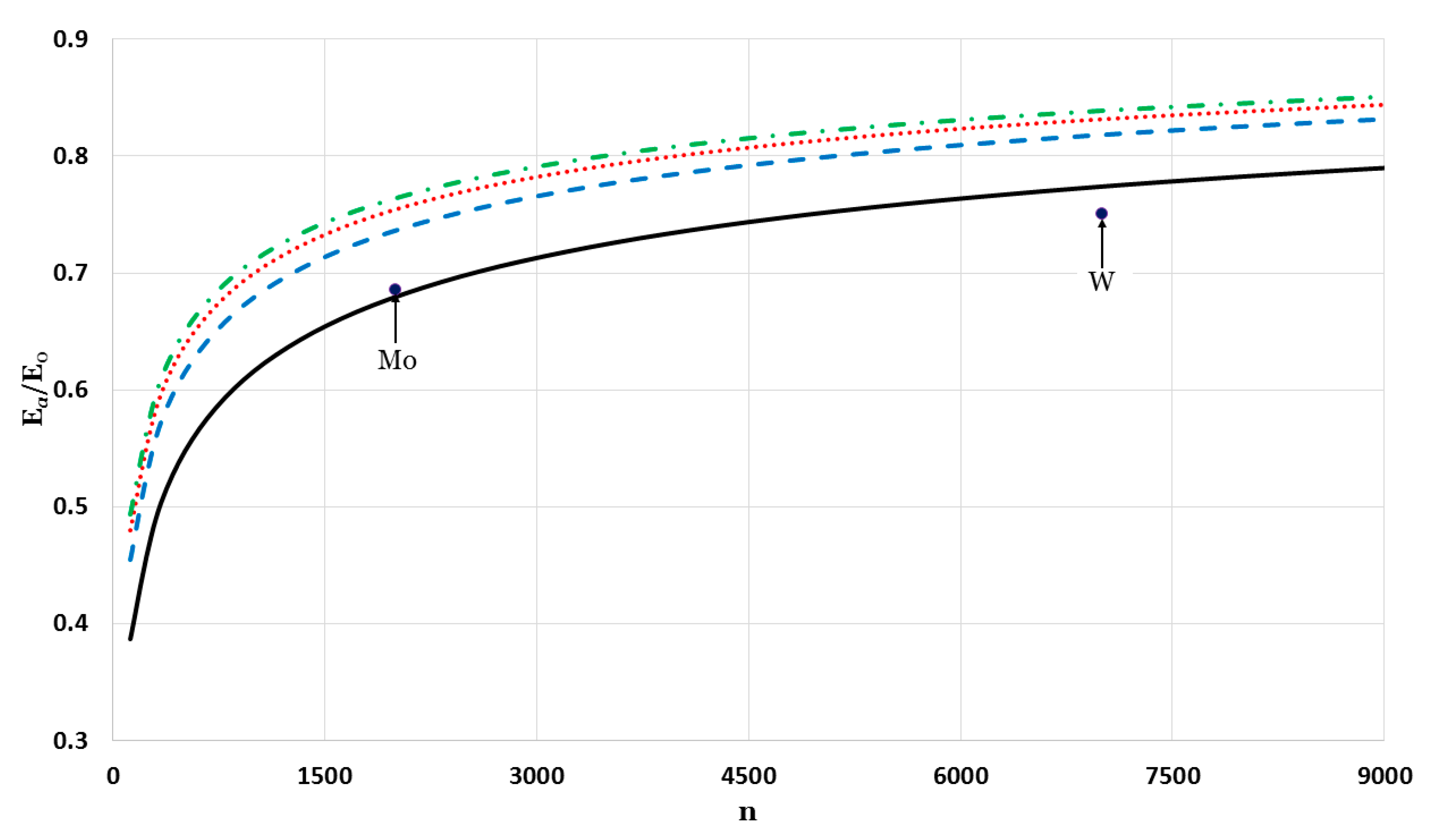
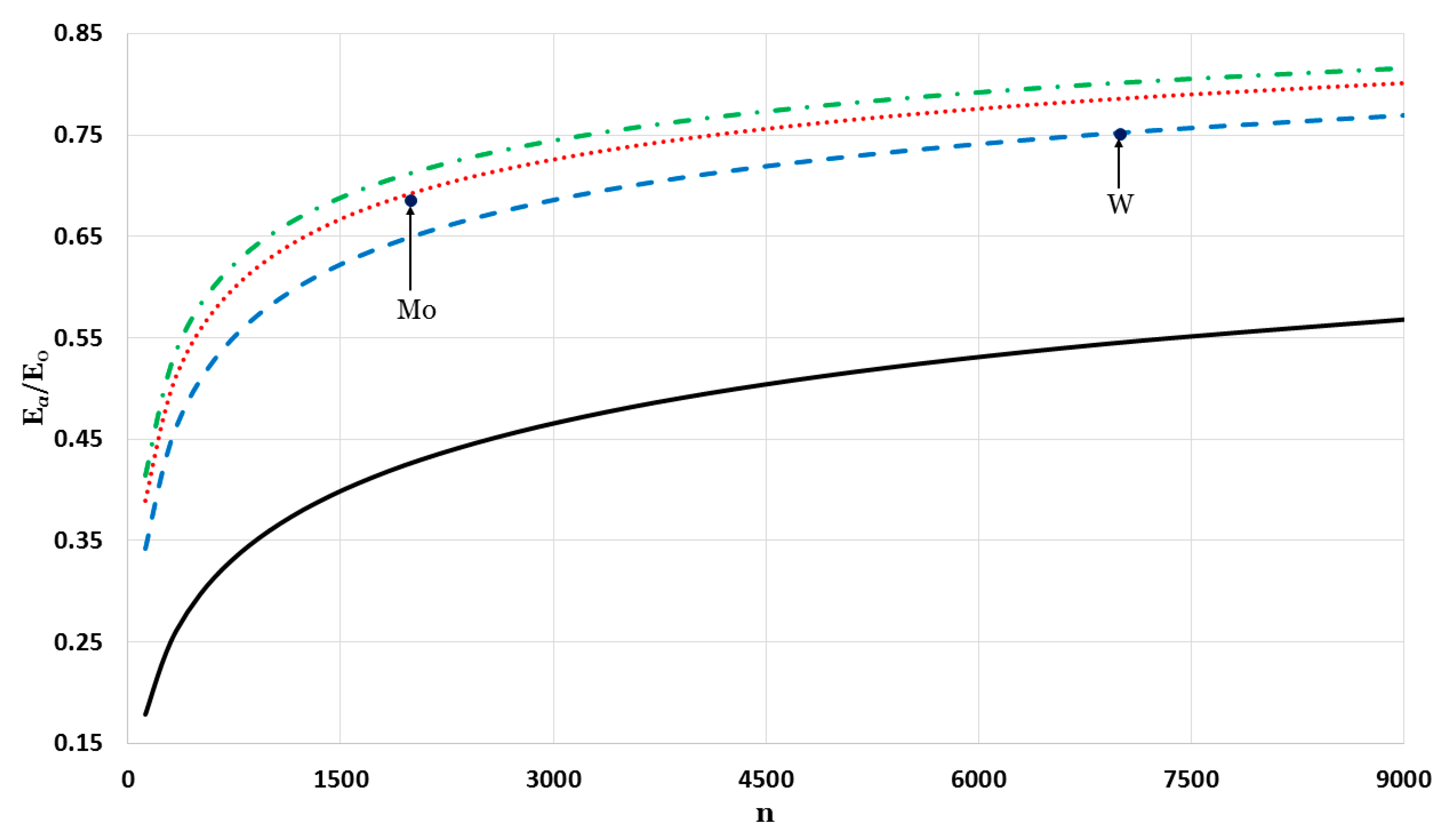
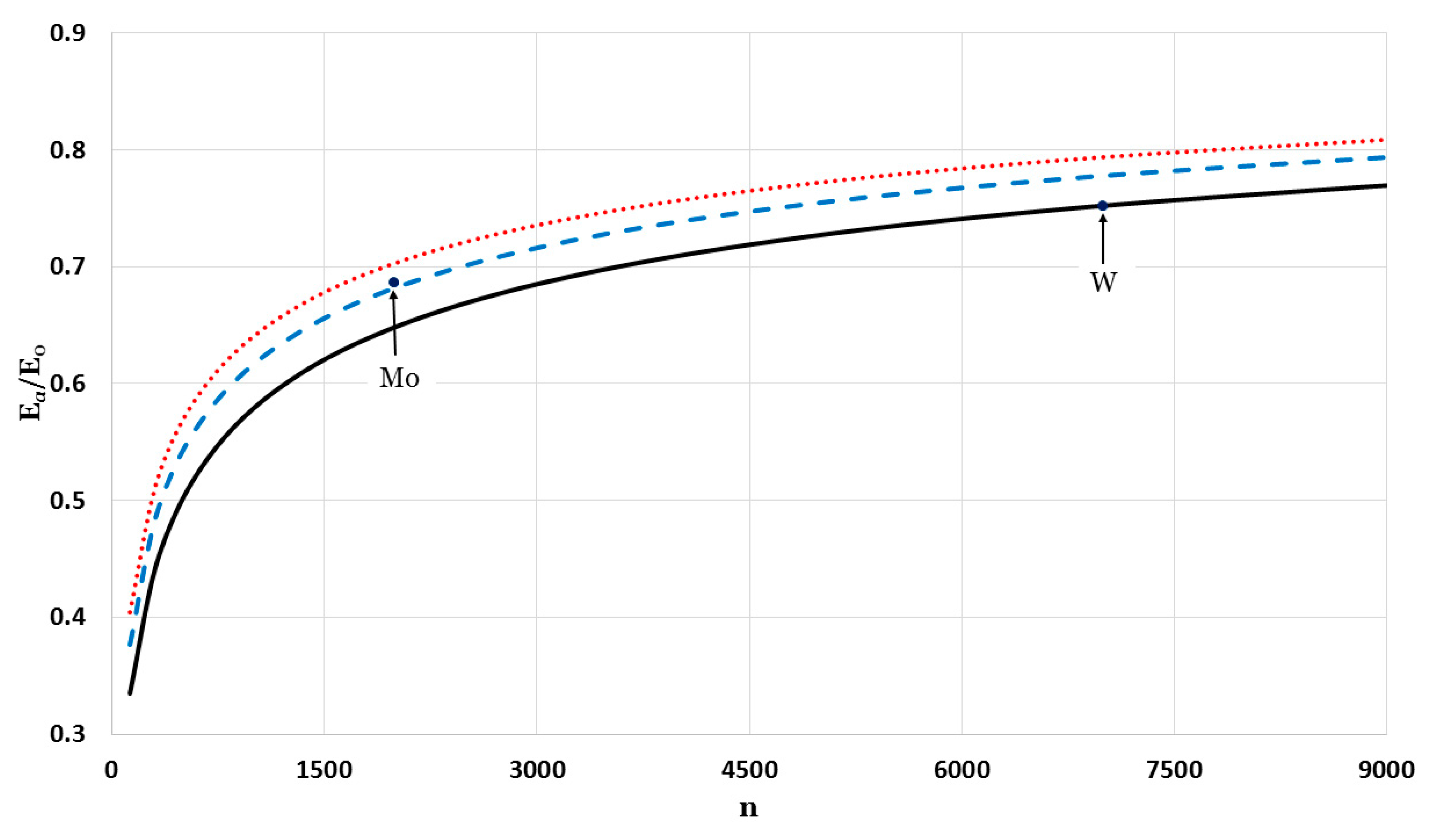
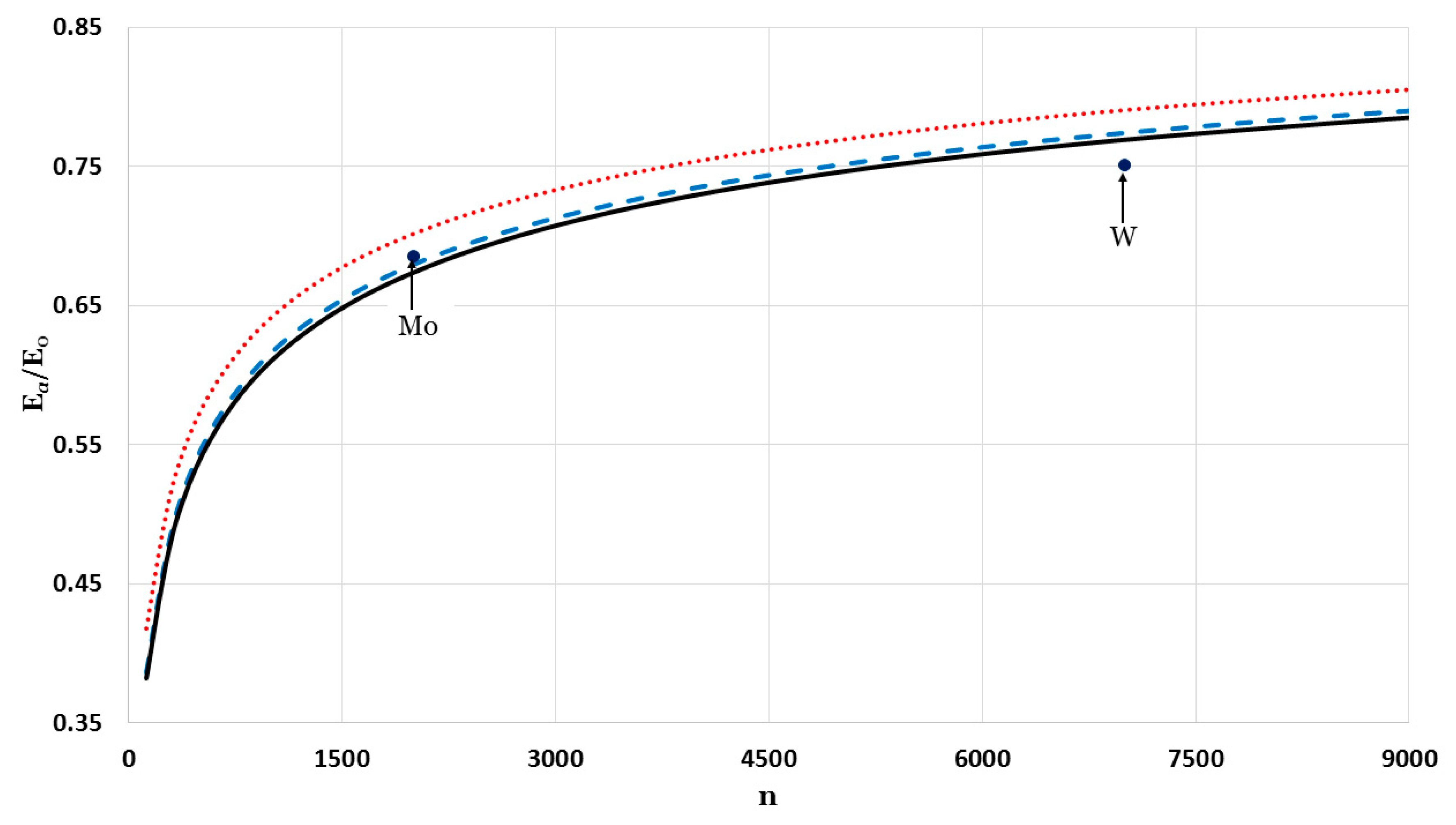
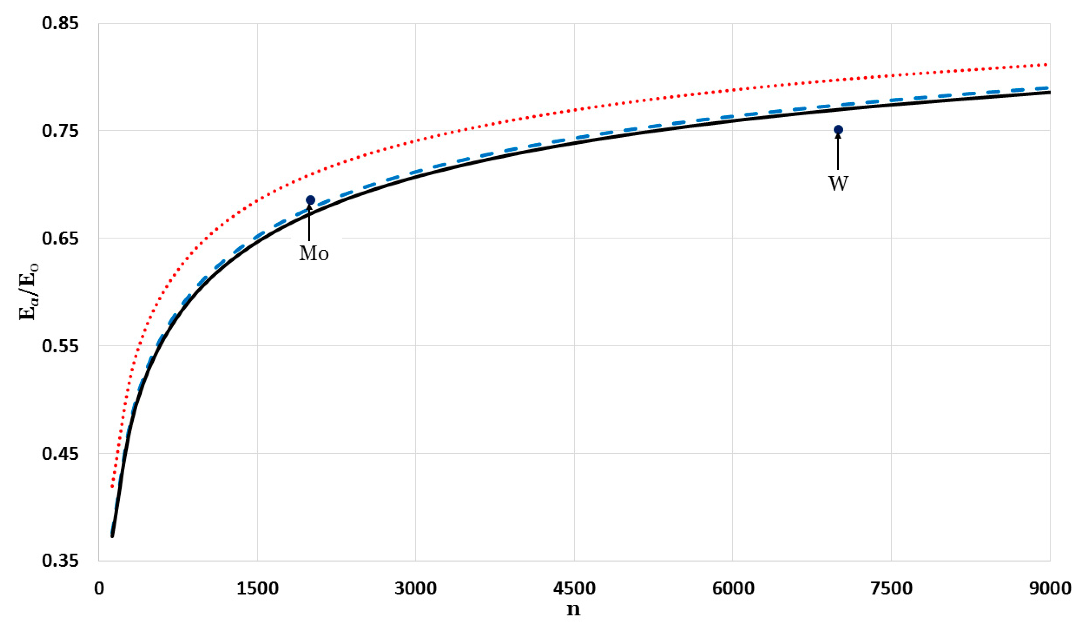
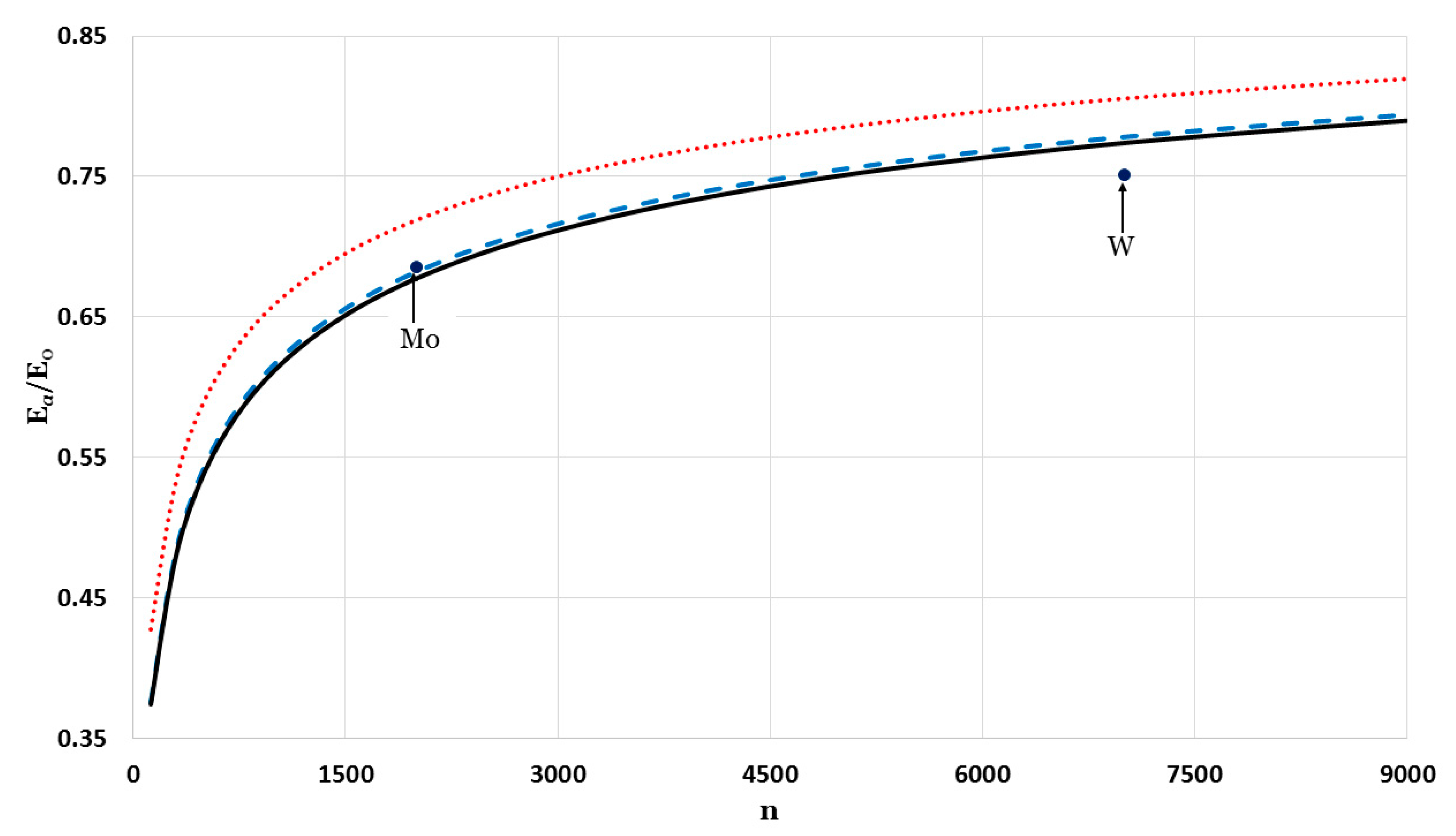
The relative cohesive energy of metallic nanoparticles in a face-centered cubic structure as a function of the number of atoms $n$ was calculated by using the generalized Morse potential function for different values of $m$ and a fixed value of $\alpha$: $\alpha =2.4$ in Figure 5 and $\alpha =2$ in Figure 6. Additionally, the calculated relative cohesive energy of the nanoparticles with a face-centered cubic structure is comparable to the experimental values of the relative cohesive energy of Mo (−410 kJ/mol for $n=2000$ atoms [23] and −598 kJ/mol for bulk [24]) and W nanoparticles (−619 kJ/mol for $n=7000$ atoms [23] and −824 kJ/mol for bulk [24]). The calculations show the size dependence of the relative cohesive energy of the metallic nanoparticles. The values of relative cohesive energy were obtained from Figure 5 and Figure 6 for $n=2000$ and $7000$ atoms and summarized in

Table 1. The relative cohesive energy of nanoparticles in a face-centered cubic structure includes $n=2000$ and $7000$ atoms for different values of $m$ and $\alpha$.

$\mathit{m}$	${\mathit{E}}_{\mathit{a}}\mathbf{/}{\mathit{E}}_{\mathbf{0}}$
	$\mathit{n} \mathbf{=} \mathbf{2000}$		$\mathit{n} \mathbf{=} \mathbf{7000}$
	$\mathit{\alpha } \mathbf{=} \mathbf{2.4}$	$\mathit{\alpha } \mathbf{=} \mathbf{2}$	$\mathit{\alpha } \mathbf{=} \mathbf{2.4}$	$\mathit{\alpha } \mathbf{=} \mathbf{2}$
2	0.427	0.679	0.542	0.774
3	0.648	0.738	0.750	0.818
4	0.691	0.755	0.784	0.832
5	0.711	0.764	0.801	0.839

. As seen in Table 1, the calculated values of the relative cohesive energy increased with the parameter $m$, due to the repulsive interaction becoming stiffer with $m$ (as seen in Figure 1). The calculated relative cohesive energies agreed with the experimental values for Mo nanoparticle when ($\alpha =2.4$, $m=2$) and ($\alpha =2$, $m=4$). On the other hand, when ($\alpha =2$, $m=3$) the calculated relative cohesive energy agreed with the experimental value for W nanoparticles.

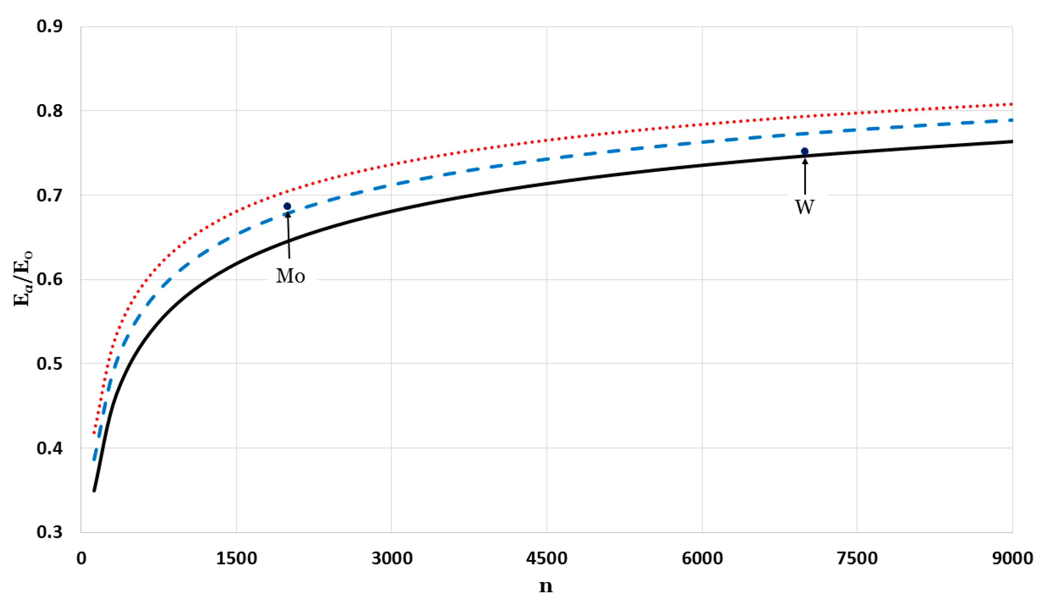
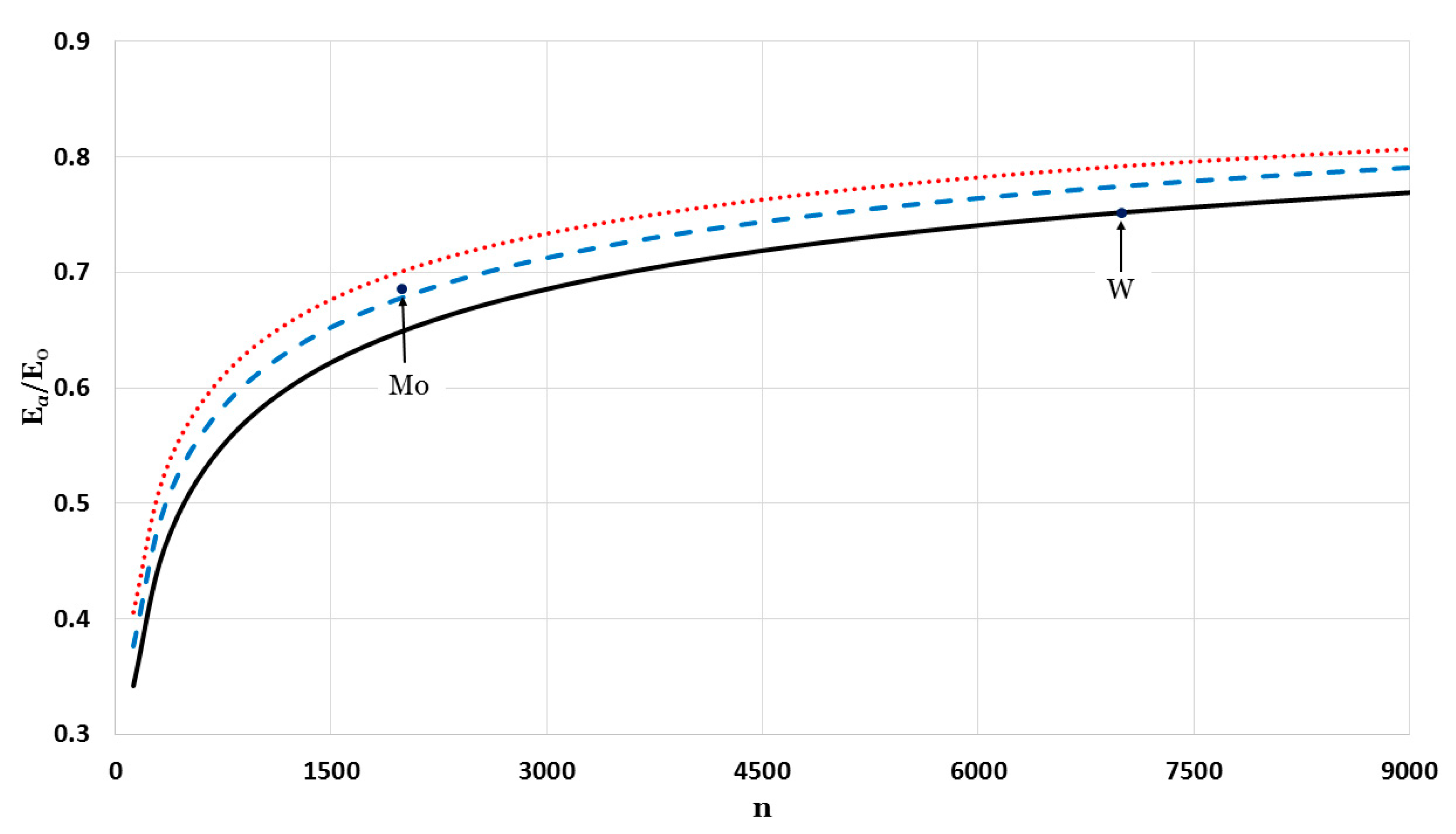
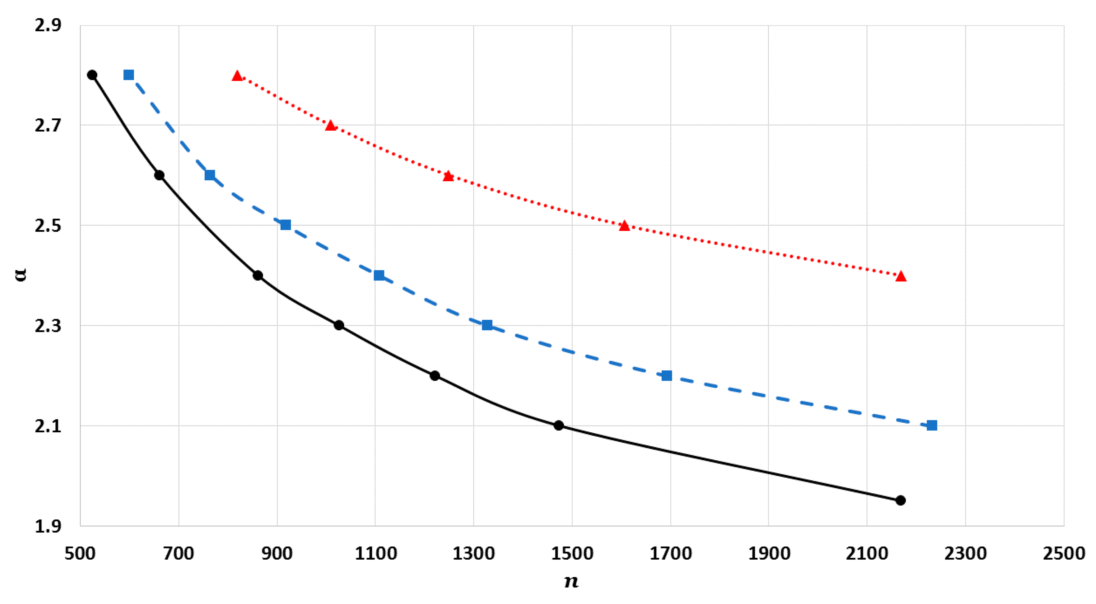
The potential function that is used to calculate the cohesive energy depends on two parameters, $m$ and $\alpha$. Different values of the parameter $m$ gave different forms of the potential functions (as seen in Figure 1). Consequently, the value of the parameter $\alpha$ will depend on type, structure, and value of $m$. The relative cohesive energies were calculated for a fixed value of $m$ and different values of $\alpha$: Figure 7 (for $m=2$), Figure 8 (for $m=3$), and Figure 9 (for $m=4$). As seen in Figure 7, Figure 8 and Figure 9, different values of $\alpha$ and $m$ for the potential function, as summarized in Figure 10, can be used to calculate the relative cohesive energies that are in agreement with the experimental values of Mo and W nanoparticles. The calculations show that the nanoparticles can be stable with a small value of $m$ and a large value of $\alpha$ (due to the softening of the repulsive force in the potential function [13]) or with a large value of $m$ and small value of $\alpha$ (due to the strong attractive force in the potential function, which is discussed later in the article).

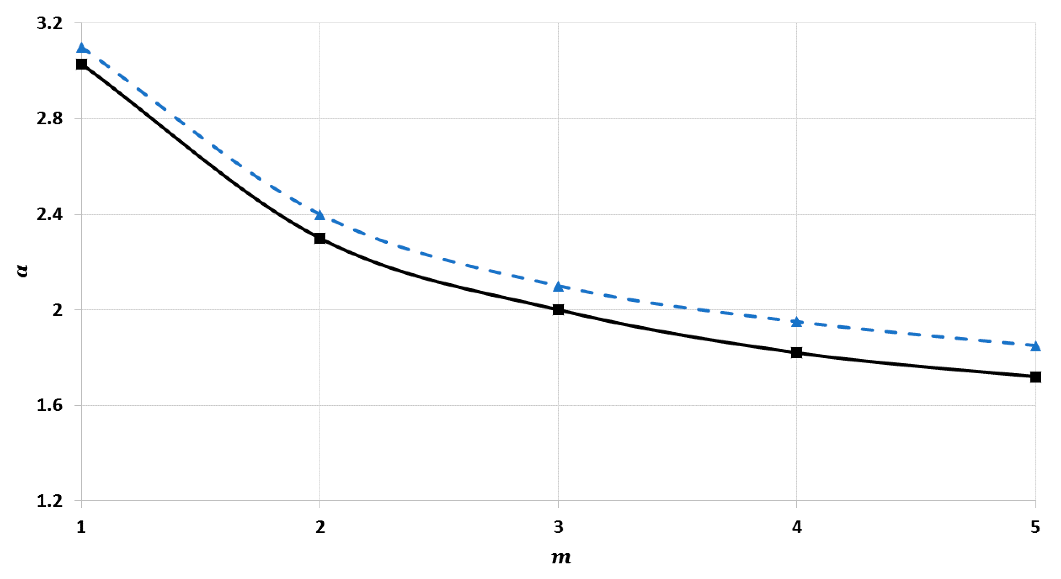
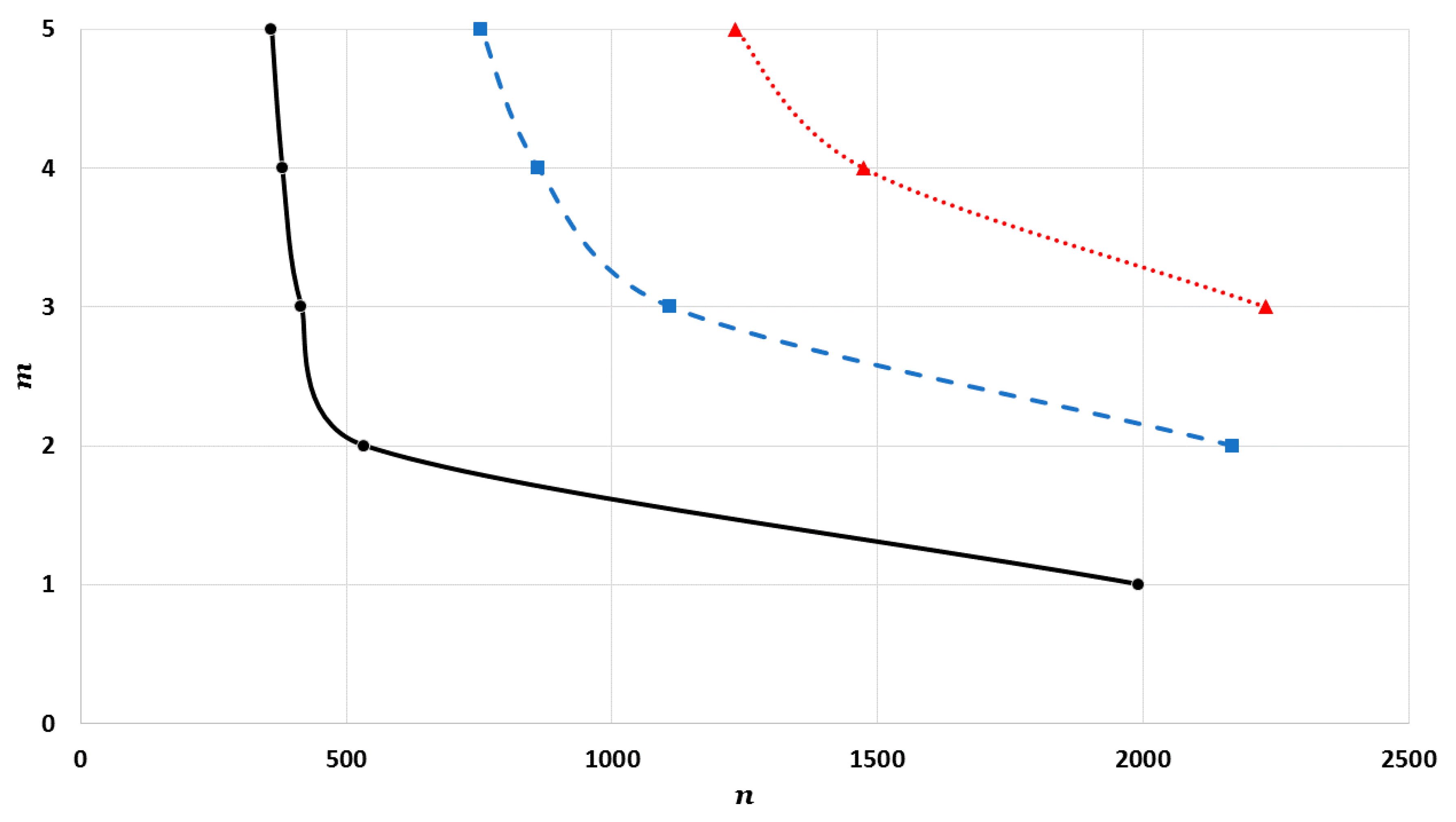
From another perspective, it was also found that the nanoparticles can be stable with a different number of atoms $n$ with the same cohesive energy if the values of $m$ and $\alpha$ of the potential function are changed, as seen in Figure 11 (shows the relation between $n$ and $m$ for different values of $\alpha$) and Figure 12 (shows the relation between $n$ and $\alpha$ for different values of $m$). Both figures show that the nanoparticles can be stabilized with a larger number of atoms having the same cohesive energy if the value of $m$ is increased and the value of $\alpha$ is decreased. This result confirms that the long-range attractive force in the potential function plays an important role in the stability of the nanoparticles.

The stability of nanoparticles is a result of the balance between repulsive interactions and attractive interactions. It was found that the stability of nanoparticles using the Morse potential function ($m=1$) is due to the soft repulsive force and weak attractive force [13]. This type of potential does not allow more bonds to form for each atom in the nanoparticle with distant surrounding atoms. Thus, only the few nearest surrounding atoms contribute to the stability of the nanoparticles. The curves in Figure 13 represent the potential functions with different values of $m$ and $\alpha$ that agree with the experimental value of the relative cohesive energy for Mo nanoparticles (as seen in Figure 10). As it is clear in Figure 10, when the parameter $m$ in the generalized Morse potential function increases, the value of the $\alpha$ parameter becomes lower. Consequently, the repulsive interaction becomes stronger and the range of the attractive interaction becomes wider. However, the change in the attractive interaction range is weak when $m\ge 3,$ due to the convergence in the $\alpha$ values. The enlargement of the attractive interaction range in the generalized potential function allows the atoms in the nanoparticles to have more bonds with the distant surrounding atoms. Consequently, the extra bonds play an important role in the stability of the nanoparticle.

The effect of nanoparticle structure in the cohesive energy was studied for different values of $\alpha$ and $m$ such that: $\alpha =2.4$ and $m=2$ in Figure 14, $\alpha =2.1$ and $m=3$ in Figure 15, and $\alpha =1.95$ and $m=4$ in Figure 16. The calculated cohesive energies for a simple cubic structure are more obvious than body-centered cubic and face-centered cubic structures as predicted in other work [12].

Melting point $T_m$ is a size-dependent property of nanoparticles [4,6,9]. Li et al. [25] found that the cohesive energy is positively proportional to the melting point of the materials ($T_m/T_{mbulk}=E_a/E_0$). Therefore, the melting point of nanoparticles as a function of the number of atoms $n$ can be calculated using Equation (8), as follows:

$$\frac{T_m}{T_{mbulk}}=\frac{P_0}{2m}{\displaystyle \sum _{k=1}^{2m}}{\left(-1\right)}^k\left(2m-\left(k-1\right)\right)A_k\left(r_0^{*}\right).$$

(9)

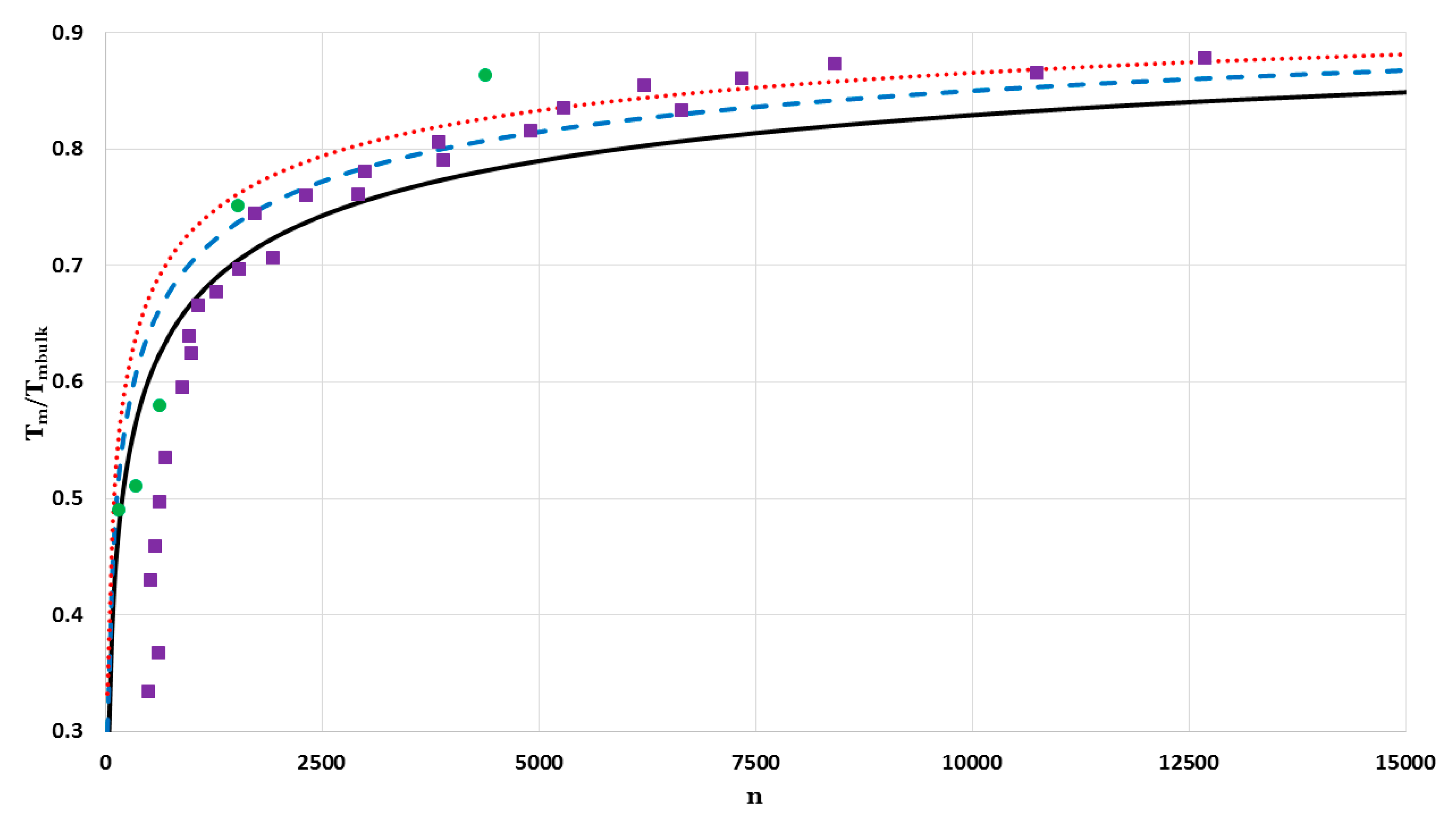
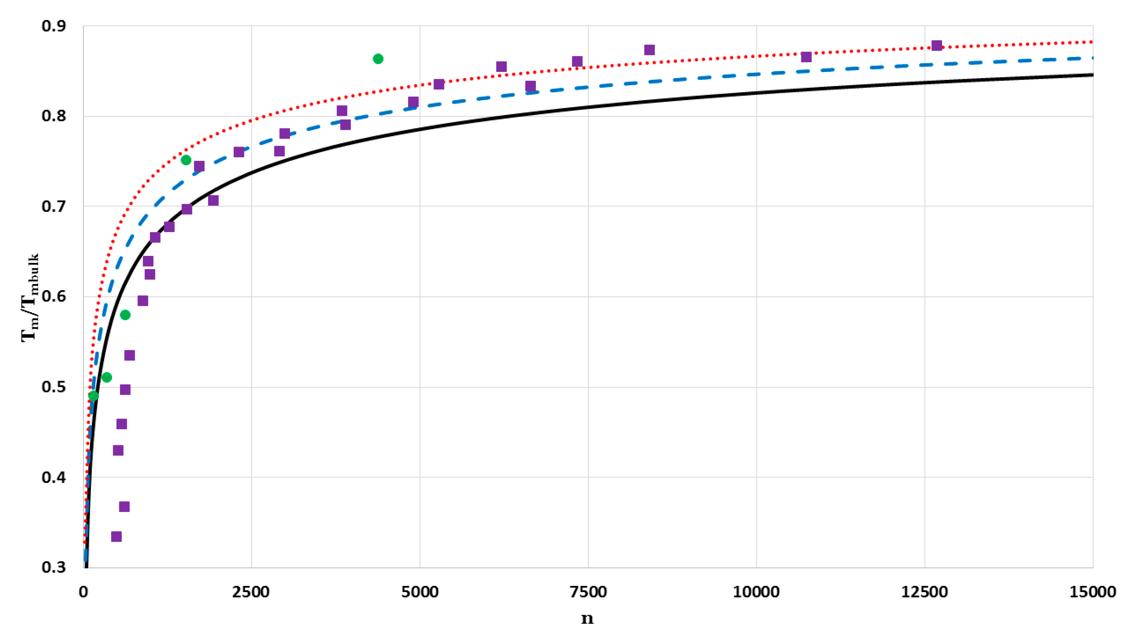
The values of $T_m/T_{mbulk}$ of nanoparticles in a face-centered cubic structure as a function of the number of atoms $n$ are calculated for a fixed value of $m$ and different values of $\alpha$: Figure 17 (for $m=2$) and Figure 18 (for $m=3$). The calculated values of $T_m/T_{mbulk}$ are compared by two different sets of experimental data of melting points of Au (the mass density is $\rho =18.4\mathrm{g}/{\mathrm{c}\mathrm{m}}^3$ [26] and the bulk melting point is $T_{mbulk}=1337.3\mathrm{K}$ [27]) nanoparticles in a face-centered cubic structure. The first set of the experimental data for melting points of Au measured by using a scanning electron-diffraction technique for nanoparticles on the amorphous carbon substrate [27]. The second set of the experimental data for melting points of silica-encapsulated Au nanoparticle measured by using a differential thermal analysis (DTA) coupled to thermal gravimetric analysis (TGA) techniques [28]. The melting points of Au nanoparticles in both sets of the experimental data are determined by their diameters $D$. The number of atoms $n$ of Au nanoparticles in a face-centered cubic structure with given diameters can be determined through the relation: $n=0.74{\left(D/d\right)}^3+1.82{\left(D/d\right)}^2$ [9,29] (where $d\left(=\sqrt{2}/2a\right)$ is the atomic diameter and $a$ is the lattice constant). The calculated values of $T_m/T_{mbulk}$ agree with the first set of the experimental data when $n\ge 1000$ atoms ($D\ge 3\mathrm{nm}$) with little deviation when $n<1000$ atoms ($D<3\mathrm{nm}$). The first set of the experimental data shows less values of melting points than those that are predicted by the model. The deviation arises due to the substrate effect on the melting point of very small Au nanoparticles [30]. In the contrast, the silica shell had a small effect on the melting point of small Au nanoparticles, where the nanoparticles are considered as individual particles [9,28]. Therefore, the predicted values of $T_m/T_{mbulk}$ agree with the experimental data of the second set when $n<1500$ atoms ($D<3.5\mathrm{nm}$).

5. Conclusions

In conclusion, the generalized Morse potential function for different values of $m$ was used to account for the size dependence of the cohesive energy for different cubic metals: Simple cubic, body-centered cubic, and face-centered cubic structures. The generalized Morse potential function with $m=3$ was used to predict the experimental values of the cohesive energy of W nanoparticles when $\alpha =2$ and Mo nanoparticles when $\alpha =2.1$. If the value of $\alpha$ is approximated to be 2, then the generalized Morse potential function with $m=3$ will have the following form:

$$U_{GMij}=\frac{D}{3}\{e^{-12\left(\frac{r_{ij}}{r_0}-1\right)}-2e^{-10\left(\frac{r_{ij}}{r_0}-1\right)}+3e^{-8\left(\frac{r_{ij}}{r_0}-1\right)}-4e^{-6\left(\frac{r_{ij}}{r_0}-1\right)}+5e^{-4\left(\frac{r_{ij}}{r_0}-1\right)}-6e^{-2\left(\frac{r_{ij}}{r_0}-1\right)}\}.$$

(10)

The above potential function contains the following terms, $e^{-12\left(\frac{r_{ij}}{r_0}-1\right)}$ and $e^{-6\left(\frac{r_{ij}}{r_0}-1\right)}$, that are equivalent to the Pauli repulsion and attractive dipole potentials, respectively, as in the Lennard–Jones potential proposed by Lim [21,22]. Consequently, the generalized Morse potential function with $m=3$ can be the suitable potential to calculate the cohesive energy of nanoparticles. The stability of nanoparticles using a generalized Morse potential function with higher values of $m$ (such as $m=3$) and low values of $\alpha$ (such as $\alpha \approx 2$) is due to the enlargement in the attractive interaction range rather than the softening of the repulsive interaction. The generalized Morse potential function with different values of $m$ and $\alpha$ were used to calculate the melting point of nanoparticles in a face-centered cubic structure. The model using the generalized Morse potential function showed ability to predict the experimental data of melting points of Au nanoparticles with neglecting any surrounding effects, such as the effect of the substrate on the melting point of small Au nanoparticles.

A Lennard–Jones potential function with an additional two long-range attractive terms was proposed to calculate the energy bands of diatomic molecules [31,32]. Therefore, adding extra terms can also be applied to the Lennard–Jones potential function (as the generalized Morse potential function with $m=3$) to predict the experimental values of cohesive energy of W and Mo nanoparticles and the melting point of Au nanoparticles in face-centered cubic structures.

References

- Qi, W.H.; Wang, M.P.; Zhou, M.; Hu, W.Y. Surface-Area-Difference Model for Thermodynamic Properties of Metallic Nanocrystals. J. Phys. D 2005, 38, 1429–1436. [Google Scholar] [CrossRef]
- Kittel, C. Introduction to Solid State Physics, 8th ed.; Wiley: New York, NY, USA, 2005. [Google Scholar]
- Qi, W.H.; Wang, M.P.; Xu, G.Y. The Particle Size Dependence of Cohesive Energy of Metallic Nanoparticles. Chem. Phys. Lett. 2003, 372, 632–634. [Google Scholar] [CrossRef]
- Qi, W.H.; Wang, M.P.; Zhou, M.; Shen, X.Q.; Zhang, X.F. Modeling Cohesive Energy and Melting Temperature of Nanocrystals. J. Phys. Chem. Solids 2006, 67, 851–855. [Google Scholar] [CrossRef]
- Liu, C.; Qi, W.; Ouyang, B.; Wang, X.; Huang, B. Predicting the Size- and Shape-Dependent Cohesive Energy and Order-Disorder Transition Temperature of Co-Pt Nanoparticles by Embedded-Atom-Method Potential. J. Nanosci. Nanotechnol. 2013, 13, 1261–1264. [Google Scholar] [CrossRef] [PubMed]
- Ouyang, G.; Yang, G.; Zhou, G. A Comprehensive Understanding of Melting Temperature of Nanowire, Nanotube and Bulk Counterpart. Nanoscale 2012, 4, 2748–2753. [Google Scholar] [CrossRef]
- Li, X. Modeling the Size- and Shape-Dependent Cohesive Energy of Nanomaterials and its Applications in Heterogeneous Systems. Nanotechology 2014, 25, 185702. [Google Scholar] [CrossRef] [PubMed]
- Safaei, A. The Effect of the Averaged Structural and Energetic Features on the Cohesive Energy of Nanocrystals. J. Nanopart. Res. 2010, 12, 759–776. [Google Scholar] [CrossRef]
- Safaei, A. Shape, Structural, and Energetic Effects on the Cohesive Energy and Melting Point of Nanocrystals. J. Phys. Chem. C 2010, 114, 13482–13496. [Google Scholar] [CrossRef]
- Qi, W.H.; Wang, M.P.; Hu, W.Y. Calculation of the Cohesive Energy of Metallic Nanoparticles by the Lennard–Jones potential. Mater. Lett. 2004, 58, 1745–1749. [Google Scholar] [CrossRef]
- Nayak, P.; Naik, S.R.; Sar, D.K. Improved Cohesive Energy of Metallic Nanoparicles by Using L-J Potential with Structural Effect. Iran. J. Sci. Technol. Trans. Sci. 2019, 43, 2705–2711. [Google Scholar] [CrossRef]
- Barakat, T.; Al-Dossary, O.M.; Alharbi, A.A. The Effect of Mie-Type Potential Range on the Cohesive Energy of Metallic Nanoparticles. Int. J. Nanosci. 2007, 6, 461–466. [Google Scholar] [CrossRef]
- Al-Dossary, O.M.; Al Rsheed, A. The Effect of the Parameter α of Morse Potential on Cohesive Energy. J. King Saud Univ.–Sci. 2020, 32, 1147–1151. [Google Scholar] [CrossRef]
- Hu, Z.; Zhang, L.; Jiang, J. Development of a Force Field for Zeolitic Imidazolate Framework-8 with Structural Flexibility. J. Chem. Phys. 2012, 136, 244703. [Google Scholar] [CrossRef] [PubMed]
- Ward, D.K.; Zhou, X.; Wong, B.M.; Doty, F.P. A Refined Parameterization of the Analytical Cd-Zn-Te Bond-Order Potential. J. Mol. Model. 2013, 19, 5469–5477. [Google Scholar] [CrossRef]
- Mie, G. Zur Kinetischen Theorie der Einatomigen Körper. Ann. Phys. (Leipzig) 1903, 11, 657–697. [Google Scholar] [CrossRef] [Green Version]
- Morse, P.M. Diatomic Molecules According to the Wave Mechanics. II. Vibrational Levels. Phys. Rev. 1929, 34, 57–64. [Google Scholar] [CrossRef]
- Le Roy, R.J.; Huang, Y.; Jary, C. An Accurate Analytic Potential Function for Ground-State N2 from a Direct-Potential-Fit Analysis of Spectroscopic Data. J. Chem. Phys. 2006, 125, 164310. [Google Scholar] [CrossRef]
- Li, H.; Roy, P.N.; Le Roy, R.J. Analytic Morse/long-range potential energy surfaces and predicted infrared spectra for CO2–H2. J. Chem. Phys. 2010, 132, 214309. [Google Scholar] [CrossRef] [Green Version]
- Girifalco, L.A.; Weizer, V.G. Application of the Morse Potential Function to Cubic Metals. Phys. Rev. 1959, 114, 687–690. [Google Scholar] [CrossRef]
- Lim, T.C. The Relationship Between Lennard-Jones (12–6) and Morse Potential Functions. Z. Naturforschung A 2003, 58, 615–617. [Google Scholar] [CrossRef]
- Lim, T.C. Long Range Relationship Between Morse and Lennard–Jones potential Energy Functions. Mol. Phys. 2007, 105, 1013–1018. [Google Scholar] [CrossRef]
- Kim, H.K.; Huh, S.H.; Park, J.W.; Jeong, J.W.; Lee, G.H. The Cluster Size Dependence of Thermal Stabilities of Both Molybdenum and Tungsten Nanoclusters. Chem. Phys. Lett. 2002, 354, 165–172. [Google Scholar] [CrossRef]
- Edgar, E.L. Periodic Table of the Elements; Version 1.1.; Ptable: Gaston, OR, USA, 1993. [Google Scholar]
- Li, J.H.; Liang, S.H.; Guo, H.B.; Liu, B.X. Four-Parameter Equation of State of Solids. Appl. Phys. Lett. 2005, 87, 194111. [Google Scholar] [CrossRef]
- Haynes, W.M. Thermal and Physical Properties of Pure Metals. In CRC Handbook of Chemistry and Physics; Internet Version 2005; Lide, D.R., Ed.; CRC Press: Boca Raton, FL, USA, 2005. [Google Scholar]
- Buffat, P.A.; Borel, J.P. Size Effect on the Melting Temperature of Gold Particles. Phys. Rev. A 1976, 13, 2287–2298. [Google Scholar] [CrossRef] [Green Version]
- Dick, K.; Dhanasekaran, T.; Zhang, Z.; Meisel, D. Size-Dependent Melting of Silica-Encapsulated Gold Nanoparticles. J. Am. Chem. Soc. 2002, 124, 2312–2317. [Google Scholar] [CrossRef]
- Safaei, A.; Shandiz, M.A.; Sanjabi, S.; Barber, Z.H. Modelling the Size Effect on the Melting Temperature of Nanoparticles, Nanowires and Nanofilms. J. Phys. Condens. Matter 2007, 19, 216216. [Google Scholar] [CrossRef]
- Lee, J.; Nakamoto, M.; Tanaka, T. Thermodynamic Study on the Melting of Nanometer-Sized Gold Particles on Graphite Substrate. J. Mater. Sci. 2005, 40, 2167–2171. [Google Scholar] [CrossRef]
- Le Roy, R.J.; Dattani, N.S.; Coxon, J.A.; Ross, A.J.; Crozet, P.; Linton, C. Accurate Analytic Potentials for Li2() and Li2() from 2 to 90 Å, and the Radiative Lifetime of Li(2p). J. Chem. Phys. 2009, 131, 204309. [Google Scholar] [CrossRef]
- Coxon, J.A.; Hajigeorgiou, P.G. The Ground Electronic State of the Cesium Dimer: Application of a Direct Potential Fitting Procedure. J. Chem. Phys. 2010, 132, 094105. [Google Scholar] [CrossRef] [PubMed]
Figure 1.
Generalized Morse potential curves for a fixed value of and different values of : 1 (black solid line), 2 (blue dashed line), 3 (green dashed-dotted line), 4 (red dotted line), and 5 (purple dashed-dotted-dotted line).
Figure 2.
The variation of for a face-centered cubic metal with the parameter for , where the blue solid line represents , the black dashed line represents , the red dashed-dotted line represents , and the orange dotted line represents .
Figure 3.
The variation of for a face-centered cubic metal with the parameter for , where the blue solid line represents , the black dashed line represents , the yellow dotted line represents , the green long-dashed-dotted line represents , the orange dashed-dotted-dotted line represents , and the red dashed-dotted line represents .
Figure 4.
The variation of for a face-centered cubic metal with the parameter for , where the blue solid line represents , the black medium dashed line represents , the yellow dotted line represents , the red dashed-dotted line represents , the orange dashed-dotted-dotted line represents , the gray long-dashed line represents , the purple short-dashed line represents , and the green long-dashed-dotted line represents .
Figure 5.
The variation of the relative cohesive energy of nanoparticles in a face-centered cubic structure as function of the number of atoms for and different values of : 2 (black solid line), 3 (blue dashed line), 4 (red dotted line), and 5 (green dashed-dotted line). The experimental values [23,24] are denoted by dark blue circles.
Figure 6.
Figure 7.
The variation of the relative cohesive energy of nanoparticles in a face-centered cubic structure as function of the number of atoms for and different values of : 2.3 (black solid line), 2.4 (blue dashed line), and 2.4 (red dotted line). The experimental values [23,24] are denoted by dark blue circles.
Figure 8.
The variation of the relative cohesive energy of nanoparticles in a face-centered cubic structure as function of the number of atoms for and different values of : 2.0 (black solid line), 2.1 (blue dashed line), and 2.2 (red dotted line). The experimental values [23,24] are denoted by dark blue circles.
Figure 9.
The variation of the relative cohesive energy of nanoparticles in a face-centered cubic structure as function of the number of atoms for and different values of : 2.05 (black solid line), 1.95 (blue dashed line), and 1.85 (red dotted line). The experimental values [23,24] are denoted by dark blue circles.
Figure 10.
The relation between the values of and used to calculate the relative cohesive energies in agreement with the experimental values can be seen: (a) For the Mo nanoparticles (0.686 for atoms [23,24]), as represented by the blue dashed line and triangles, and (b) for the W nanoparticles (0.751 for atoms [23,24]), as represented by the black solid line and squares for a face-centered cubic structure. The values for were obtained from previous works [13].
Figure 11.
The variation of with the number of atoms for nanoparticles, having relative cohesive energies of approximately 0.686, and different values of : 3.1 (black solid line and circles), 2.1 (blue dashed line and squares), and 2.4 (red dotted line and triangles).
Figure 12.
The variation of with the number of atoms for nanoparticles, having relative cohesive energies of approximately 0.686, and for different values of : 4 (black solid line and circles), 3 (blue dashed line and squares), and 2 (red dotted line and triangles).
Figure 13.
Generalized Morse potential curves for different values of and , where the black solid line represents and (Morse potential function [13]), the blue dashed line represents and , the red dotted line represents 3 and , the green dashed-dotted line represents and , and the purple long dashed-dotted-dotted line represents and .
Figure 14.
The variation of the relative cohesive energy as function of the number of atoms (where and ) for different cubic structures of nanoparticles: A body-centered cubic structure (black solid line), a face-centered cubic structure (blue dashed line), and a simple cubic structure (the red dotted line). The experimental values [23,24] are denoted by dark blue circles.
Figure 15.
Figure 16.
Figure 17.
The variation of of nanoparticles in a face-centered cubic structure as function of the number of atoms for and different values of : 2.6 (black solid line), 2.8 (blue dashed line), and 3 (red dotted line). The first set of the experimental data [27] is denoted by purple squares and the second set of the experimental data [28] is denoted by green circles.
Figure 18.
The variation of of nanoparticles in a face-centered cubic structure as function of the number of atoms for and different values of : 2.3 (black solid line), 2.5 (blue dashed line), and 2.8 (red dotted line). The first set of the experimental data [27] is denoted by purple squares and the second set of the experimental data [28] is denoted by green circles.