Self-Diagnosis of Multiphase Flow Meters through Machine Learning-Based Anomaly Detection


1
Department of Information Engineering, University of Padova, 35131 Padova (PD), Italy
2
Pietro Fiorentini S.p.A., 36057 Arcugnano (VI), Italy
3
Human Inspired Technology Research Centre, University of Padova, 35131 Padova (PD), Italy
*
Author to whom correspondence should be addressed.
Energies 2020, 13(12), 3136; https://doi.org/10.3390/en13123136
Submission received: 18 May 2020
/
Revised: 8 June 2020
/
Accepted: 12 June 2020
/
Published: 17 June 2020
(This article belongs to the Special Issue Advanced Manufacturing Informatics, Energy and Sustainability)
Abstract
:Measuring systems are becoming increasingly sophisticated in order to tackle the challenges of modern industrial problems. In particular, the Multiphase Flow Meter (MPFM) combines different sensors and data fusion techniques to estimate quantities that are difficult to be measured like the water or gas content of a multiphase flow, coming from an oil well. The evaluation of the flow composition is essential for the well productivity prediction and management, and for this reason, the quantification of the meter measurement quality is crucial. While instrument complexity is increasing, demands for confidence levels in the provided measures are becoming increasingly more common. In this work, we propose an Anomaly Detection approach, based on unsupervised Machine Learning algorithms, that enables the metrology system to detect outliers and to provide a statistical level of confidence in the measures. The proposed approach, called AD4MPFM (Anomaly Detection for Multiphase Flow Meters), is designed for embedded implementation and for multivariate time-series data streams. The approach is validated both on real and synthetic data.
1. Introduction
A Multiphase Flow Meter (MPFM) is a complex instrument employed by oil and gas companies to monitor their production. It is usually placed on top of an oil well, and it is continuously crossed by a mixture of gas, oil, and water. It allows to measure the flow in real-time, without separating the phases. The knowledge of the flow composition is crucial for the oilfield management and well productivity prediction; as a consequence, procedures for the assessment of the measuring reliability are critical.
In recent years, many efforts have been done in order to improve the MPFM performances, increasing its complexity: many sensors have been implemented on-board, improving the number of available physical variables. Unfortunately, the increased complexity is associated with a bigger set of failure types that the system can experience. The reliability of this system is crucial for every customer that consumes the supplied data for monitoring, decision-making, and control the oil production. To achieve the required reliability, the MPFM must be able to self-diagnose its sensors in an autonomous fashion.
Besides the energetic sector, data reliability is fundamental in many fields such as finance, IT, security, medical, e-commerce, agriculture, and social media. With the advent of “Industry 4.0”, the interest in accurate metrology tools has pushed many companies to develop complex measuring instruments. These sophisticated systems, which we call Complex Measuring Systems (CMSs), estimate quantities difficult to be measured combining different sensors measurements and data fusion techniques [1]. The MPFM is one example of CMSs, and therefore in the following pages the acronyms will be treated as synonyms. Although specifically developed for the MPFM, the proposed methodology could be applied to other CMSs.
Self-diagnosis capabilities can be reached in two ways: by leveraging a priori/physical knowledge of the metrology tool and the underlying measured phenomena, or by exploiting historical data and statistics/Machine Learning. In the latter case (that is the focus of this work), several algorithms can be employed, both in the realm of classification approaches and in the category of unsupervised anomaly detection methodologies. The choice mainly depends on the type of available data. In the context of MPFM, these techniques cannot be directly applied and many constrains have to be taken into account; such challenges can be summarized as follows.
- Data structure and multi-dimensionality: MPFMs are usually made up of different metrology modules that measure quantities related to distinct physical variables, and each module can have a different sampling rate. As a result, data to be monitored are a collection of multivariate and heterogeneous streaming of time-series.
- Non-stationarity: The measured process can be non-stationary, i.e., the mean and the variance of the underlying process can vary over time; in this context, historical data can be not representative of the possible system states. To overcome this issue, the monitoring agent has to find some quantities that describe the behavior of the instrument, independently on the process.
- Root cause analysis: Due to the changing environment and the complex interaction between the modules, identifying the faulty sensor/module can be a quite difficult task.
- Edge application: For most MPFMs, self-diagnosis capabilities have to be equipped on the edge, as (i) many systems have to provide data in real-time and (ii) the Internet of Things scenario [2] may not be feasible or cost-effective for many customers.
- Limited Resources: Many MPFMs have unfortunately limited computational power and memory capacity.
Given the problems previously discussed, there is a great need for developing robust algorithmic techniques for MPFM self-diagnosis that are able to (i) provide confidence intervals for the measures they produce and (ii) detect sensors/measuring modules that are proving anomalous measures. Such targets may be achieved by the usage of Anomaly Detection techniques [3]. More specifically, given the above issues and following the guidelines in [4], we define here the general requirements for real-world anomaly detection algorithm applied to the MPFMs:
- predictions must be made in real-time and on-board;
- algorithms should not rely on historical data to be trained, but it must learn from data collected on the field;
- outcomes of the anomaly detection module need to be accurate and robust, i.e., they should not be affected by changes in the underlying process;
- anomaly detection algorithms should minimize an optimal trade-off between false positives and false negatives; the optimality is defined given the application at hand;
- the computations must be as light as possible;
- the anomaly detection algorithm must handle different sampling frequencies; and
- the anomaly detection algorithm must be independent on the meter calibration settings.
The focus of this work will be to present an Anomaly Detection approach for MPFM that considers the aforementioned constraints and allows equipping the instrument with self-diagnosis capabilities. In particular, a preprocessing pipeline specifically designed for this type of meter will be shown. This will allow to (i) effectively employ computationally efficient Anomaly Detection tools and (ii) develop a powerful Root Cause Analysis algorithm. Moreover, we will test such approach exploiting real data, coming from specialized testing facilities, called flow loops. In the following we will refer to the proposed approach with the name AD4MPFM that stands for Anomaly Detection for Multiphase Flow Meters.
Preliminary results have been published in [5]; with respect to the aforementioned work, in this manuscript several additional investigations have been reported, namely, a diagnostic method for enabling Root Cause Analysis, a broader comparison of Anomaly Detection methods, and new types of considered faults and more detailed experiments.
The rest of the paper is organized as follows. Section 2 is dedicated to review the related literature, to describe the MPFM and its principles, and to highlight the novelty of the present work. The proposed approach for Anomaly Detection in MPFM is presented in Section 3, while the experimental settings are illustrated in Section 4. In Section 5, the experimental results are shown and commented, while final comments and future research directions are discussed in Section 6.
2. Premises: Literature Review, Multiphase Flow Meter, and Contribution
2.1. Data-Driven Anomaly Detection
Classically, a model-based strategy is the most natural approach to tackle the Anomaly Detection problem. However, the performances of these strategies are strongly dependent on the quality of the model they rely on. Finding a model for a MPFM can be particularly challenging, as it means (i) modeling all the measuring modules, their interaction, and the underlying process, and (ii) due to the system non-stationarity, the usage of fixed models without customization and periodic updates is hardly viable.
By exploiting the availability of historical data, a data-driven strategy is typically preferable. Data-driven approaches [6,7,8,9] aim at finding a model that best fits data without physical a priori knowledge of the process. They are usually divided into two main categories: supervised and unsupervised. Supervised methods are very powerful but need data where each sample is labeled Faulty/Non-Faulty. Unfortunately labeled datasets are hardly available: the labeling procedure is very expensive and time-consuming. A human domain expert has to manually tag the dataset with a posteriori visual inspection. However, the large number of module combinations and operating conditions makes these methods typically hardly viable.
Unsupervised techniques allow to overcome these issues. Their main benefits are [10] (i) the capacity of handling multivariate data and multi-modal distributions and (ii) the fact that they do not need labels. Unsupervised Anomaly Detection (AD) algorithms are fundamental tools to detect anomalous behavior in metrology instruments. Working in an unsupervised way, they are flexible, accurate, and highly suited for fault detection in complex systems. They are able to perceive abnormal instrument behaviors that even domain experts struggle to detect. Given the advantages described above, AD approaches have been applied in various contexts: automotive [11], biomedical instruments [12], decision support systems [13], fraud detection [14], and industrial processes [15].
In the literature there are many definitions of anomaly depending on the application of interest. Hawkins, in [16], describes an outlier in a way that seems the more appropriate to our problem:
“An outlier is an observation which deviates so much from the other observations as to arouse suspicions that it was generated by a different mechanism.”
Therefore, outliers are far and, hopefully, less than inliers. The choice on how far and how few the observations must be to be outliers is not trivial. The outlier numerosity can vary: it is reasonable to assume that anomalous observations will increase as the environment ruins the sensor. When the fault is fully developed the outliers can be a significant percentage of the total samples.
2.2. The Multiphase Flow Meter
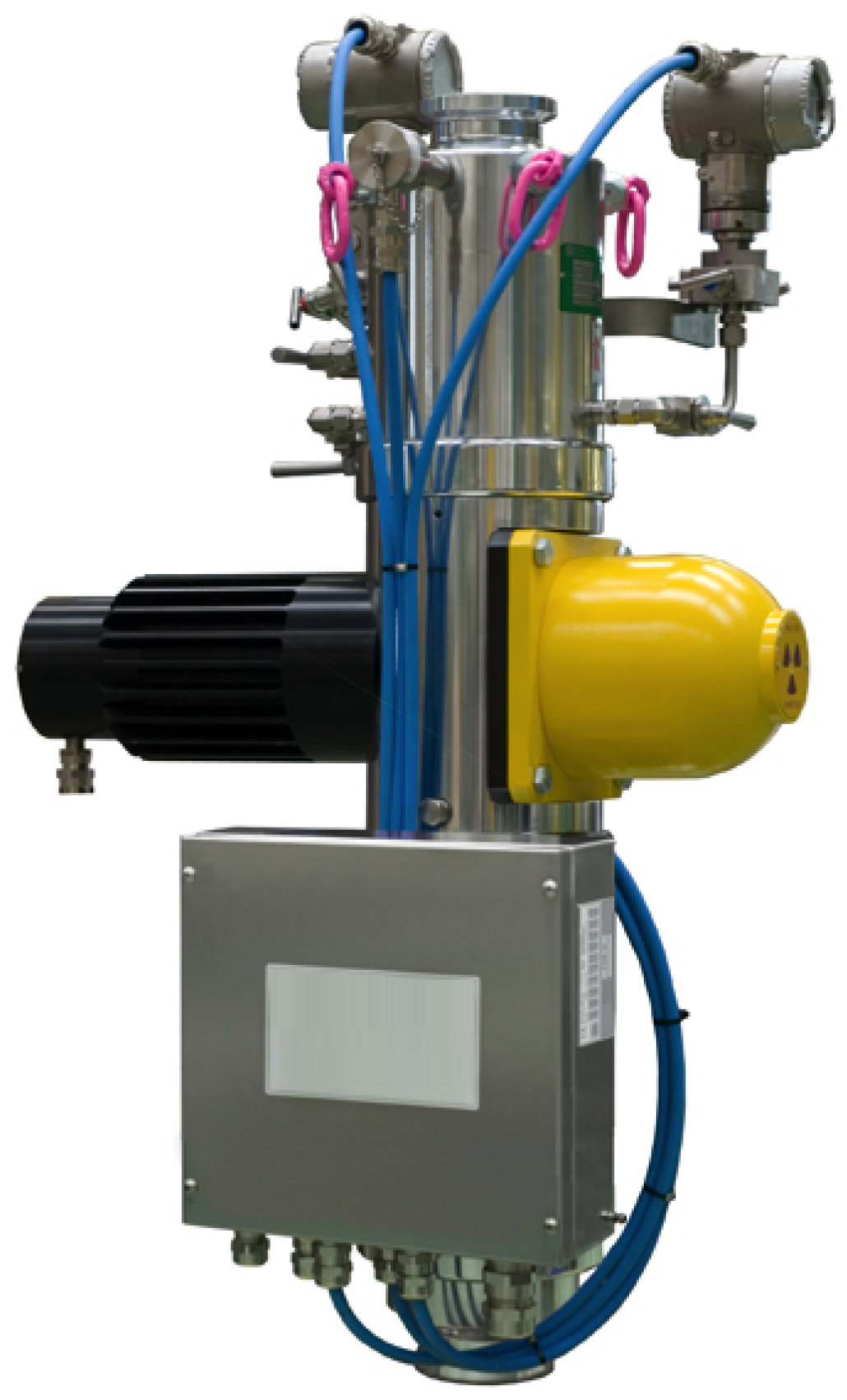
The Multiphase Flow Meter is a paradigmatic example of CMS composed of many measuring modules and requiring data fusion to provide the target measure (Figure 1).
The MPFM is an in-line measuring instrument able to quantify the individual flow rates of oil, water, and gas coming from an oil well. As it does not separate the phases, it is able to provide measures in real-time. MPFMs are employed both onshore and offshore, in topside, or subsea configuration. In this work, data have been collected using a MPFM [17], which is made in a modular way. As each module contains a specific set of sensors, in the following paragraphs the words sensor and module will be treated as synonyms.
The most common instruments employed by MPFMs are [18]:
- Venturi tube
- The Venturi tube consists of a pipe with a shrinkage in the middle, named throat. The difference between the pressure at the inlet and the pressure at the throat, called DP, is proportional to the velocity of the flow and the density of the mixture passing by. In this location, both the absolute temperature and pressure are usually measured.
- Impedance sensor
- Depending on the flow composition, it is able to work in capacitive or conductive mode, measuring respectively the permittivity and conductivity of the mixture. Multiple electrodes make up the impedance sensor; cross-correlating the measurements coming from these electrodes, it is possible to infer the velocity of the flow.
- Gamma ray densitometer
- This sensor hits the mixture with a beam of gamma rays and measures its attenuation. As the attenuation is proportional to the amount of material crossed by the beam, this sensor estimates the density of the mixture. In this work, the MPFM was equipped with a source of (Cesium) that has a half-life of almost 30 years.
2.3. Literature Review
Despite the importance of detecting malfunctions in MPFMs, the literature on self-diagnosis and AD applied to CMS is not very broad. Traditionally, CMS are monitored employing univariate control charts [22,23] that fail to capture complex data behaviors and multidimensional anomalies. Moreover, they are generally more effective in monitoring the underlying process instead of the performance of the CMS. More refined techniques that manage multivariate data are scattered among many different applications such as automotive [24], aerospace [25], chemical industry [26], Heating, Ventilating and Air Conditioning [27], energetic [28], and other industrial/manufacturing applications [29,30,31,32,33,34]. Other approaches that are similar to the one set by the CMS can be found in [35,36,37,38], where AD techniques are applied to wireless sensor networks in a non-stationary environment. Unsupervised methods able to detect the root cause of the CMS fault are, to the best of our knowledge, still missing. As stated above, the literature concerning the self-diagnosis and fault detection applied to MPFMs is at its early stages.
In general, AD detection on multivariate time series is still a quite unexplored research field. The existing literature is mainly divided into techniques applied to multivariate static datasets [39], and methods applied to univariate time-series [40].
Some of the most important multivariate static emerging techniques will be briefly described in Section 3.2.6. Concerning AD on univariate time series, we cite the following approaches. The authors of [41,42] employ a neural network to model the time-series and detect the anomaly looking at the residue: an anomaly occurs when the actual value is too far from the network prediction. In [43], the authors sequentially apply a 2D-Convolutional Neural Network in order to promptly detect the anomalies. In [44], the authors look for contextual anomalies in univariate time-series that show a strong seasonality. They decompose the series in median, seasonal, and residue, and use robust univariate AD methods on signal windows. Two interesting approaches that consider the correlation between the measures can be found in [45,46]. The last one faces a problem very similar to ours since they manage highly dynamic, correlated, and heterogeneous sensor data.
In this paper, we try to combine and to take the best from these approaches, enlarging the few unsupervised tools applied to multivariate time series. The proposed algorithm is designed to fit the MPFM requirements and characteristics described in Section 1. One of the novelty of this paper is that the AD4MPFM is able to not only detect the fault, but also to detect the root cause in an unsupervised fashion.
3. Proposed Approach: AD4MPFM
3.1. Intuition
Three key points led us to the development of AD4MPFM:
- non-stationarity of the underlying process,
- high correlation between the measuring modules, and
- need for light computations to enable edge computation.
As already mentioned, the MPFM is employed in the estimation of physical quantities that are challenging to be measured. For doing this, it might combine many measurements coming from different modules. The physical quantities to be measured might vary widely and frequently over time: this makes the use of historical data very hard. Indeed, when available, these data might not describe all the possible operating points of the MPFM. In addition, the same type of MPFM can behave differently due to different sensors calibration. Therefore, we need a monitoring algorithm that is
- independent on the process—it is able to decouple the dynamics of the measured process from the dynamics of the instrumentation, and
- independent on the calibration settings—i.e., able to auto-tune its parameters.
In MPFM, it is common to have highly correlated sensing modules: some sensing modules might measure the same physical property in order to get robust measurement or to measure derived quantities (e.g., velocity). A more interesting case is the correlation between modules that measure different physical properties: they are usually at least locally correlated because they see the same physical process (e.g., the appearance of a bubble, or the development of a slug flow) by different perspectives. In other words, at any moment the same physical phenomenon is seen by all sensors from different viewpoints. We stress that by “locally correlated” we mean correlated on a sufficiently small time interval.
A common strategy in AD [41,47] is to model the underlying process and look at the residue between the prediction and the actual value; when the residue becomes bigger than the confidence interval of the predictive model, the anomaly is detected. However, modeling a non stationary process is very complex from many points of view and, as explained above, in this context we need a computationally light model that does not need to be trained on historical data; therefore, this kind of strategy is not viable in AD for MPFM.
Although we cannot afford to model and forecast the evolution signal , we develop a different approach based on the following intuition; as the correlation between and is sufficiently high, we can think of as an approximate model for , and vice versa. Looking at the difference between correlated modules, we filter the process dynamics and we are able to analyze the instrumentation behavior. The basic assumption is that an anomaly is likely to be present when the modules disagree: it happens when the information contained in one signal differs significantly from all the other signals. This approach does not need historical data but it only needs to find a suitable way to get the difference between different sensor measurements. Obviously, the higher the correlation between the modules is, the better this kind of filter will work. If the instrumentation works in ideal way, the differences will be Gaussians.
3.2. Algorithm
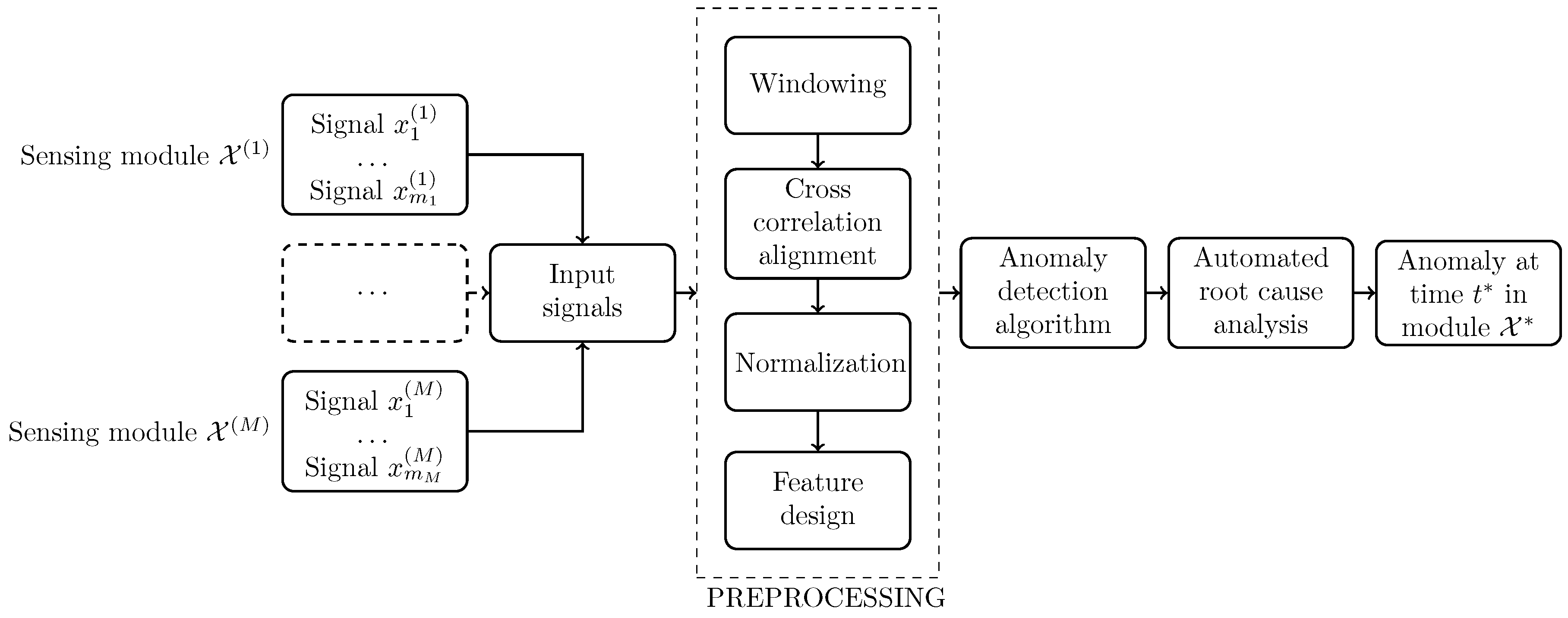
The algorithm depicted in the block diagram in Figure 2 is our proposal for AD for MPFM, namely, AD4MPFM, and it expresses the fundamental intuition detailed in the previous subsection. In this subsection, every step of this flowchart will be analyzed in detail.
3.2.1. Data collection
The first step is the collection of signals belonging to the locally correlated modules. As these modules might have different acquisition rates, a homogenization of the signals time frequencies has to be done. This can be achieved taking the mean of all the signals over the lowest sampling rate.
3.2.2. Windowing
The AD4MPFM algorithm requires fixed size batches; for this reason, the signals need to be windowed. The windowing procedure splits the initial signals into small overlapping intervals of size and time overlap .
3.2.3. Alignment
The sensing modules might have a time delay between them. This happens, for example, when they are arranged along the pipe, and therefore they experience a delay proportional to the velocity of the flow. However, the proposed feature design works best when the signals are well aligned in time and the correlation between them is sufficiently high, i.e., when the modules measure the same event at the same time. A cross correlation procedure is employed to ensure such alignment [48]: this simple choice was motivated by the computational resources constrains. Dynamic Time Warping [49] and other more sophisticated alignment procedures might not be feasible on edge implementations.
3.2.4. Normalisation
An important and simple preprocessing procedure for comparing two signals belonging to sensors that measure different physical properties, is by normalizing them. This step is very simple but quite delicate:
- Subtracting the mean and dividing by standard deviation can be dangerous, due to the possible presence of outliers. To overcome this issue, we decided to normalize each signal window by means of median and median absolute deviation.
- In order to be consistent between different windows of the same signal, we have chosen a reference window, whose scaling factors (i.e., median and median absolute deviation ) have been employed to normalize the other windows.
- Despite the outlier robustness of the median and mad, the choice of the reference batch has to be done carefully. This batch should be collected in controlled conditions, keeping attention to the possible outliers.
3.2.5. Feature Design
The next step in the AD4MPFM is to encode the previously explained insight: the features should express the difference between the informative content of the signals. Given two normalized and windowed signals and , the feature has been defined as
where K is the correlation matrix between all the signals, is the correlation coefficient between , and computed as
where is the sample mean and is the sample standard deviation of the windowed and aligned signal . The function is needed when the correlation between the signals is negative. Although other choices for making signals comparable can be employed (for example allowing a softer difference or by weighting the difference with the correlation value), we decided to adopt the procedure described above for simplicity in the edge deployment.
3.2.6. Unsupervised Anomaly Detection: Methods
Unsupervised AD algorithms can be divided into many categories depending on their working strategy. In this paper, we have chosen to compare six different AD algorithms belonging to the most important families: Proximity-Based, Linear Model, Outlier Ensembles, and Statistical methods.
Proximity-Based techniques define a data point as an outlier, if its locality (or proximity) is sparsely populated [50]. The notion of proximity can be defined on the basis of clusters, distance or density metrics. Local Outlier Factor (LOF) is the most well known algorithm of this family [51]. Following this approach, the anomaly score of a given point is function of the clustering structure in a bounded neighborhood of that observation [52]. In this paper, we have applied an optimized version of LOF named Cluster-based Local Outlier Factor (CBLOF) [52]. A simpler density technique tested in this work is Histogram-based Outlier Score (HBOS) [53]: this approach assumes the features are independent, allowing fast computations but giving up high performance. As the name of the approach says, it is based on univariate histograms constructed separately on each feature.
Linear methods assume that normal data are embedded in a lower dimensional subspace. In this subspace, outliers behave very differently from other points and it is much easier to detect them. PCA is the most famous member of this class; the main idea behind this classic method is to find a set of uncorrelated variables (named principal components), ordered by explained variability, from a dataset. The authors of [54] define the anomaly score as the distance in the principal component space previously computed. The distance in the principal component space between the anomaly and the normal instance is the anomaly score. Minimum covariance determinant [55] (MCD) is another linear method that is highly robust to outliers. Its anomaly score is based on the Mahalanobis distance from the center of the cluster.
Outlier ensembles combine the results from different models in order to create a more robust one. Isolation-based methods [56] rely on the average behavior of a number of special trees called isolation trees. This procedure tries to isolate a given observation from the rest of the data in an iterative way, making random partitions of the feature space. This method is based on the idea that outliers are easy to be isolated, while normal data tend to be inside the dataset, requiring more partitions to be isolated.
Probabilistic and statistical methods are a class of very general techniques. They usually assume an underlying data distribution. After the parameter training, the model becomes a generative model able to compute the probability of a sample to be drawn from the underlying distribution. The method that we named MAD is a multidimensional extension of the well-known control chart based on the median absolute deviation . As mean and standard deviation are very sensitive to outliers, it is common practice to set control limits on the basis of and [57] as they are much more robust. Given a window of the signal :
the anomaly score for each sample is defined by the MAD algorithm as
Note that in ideal conditions, gives a robust estimate of the Gaussian standard deviation. As the MAD algorithm is based on the median absolute deviation, its AS can be easily interpreted as the relative distance of the samples from the distribution center.
3.2.7. Unsupervised Anomaly Detection: Usage and Metrics
After the computations, a general AD algorithm returns an index that measures the abnormality level of data, namely, the anomaly score (AS) of each sample. Data with higher AS are more likely to be outliers. In order to assess which method performs better at detecting anomalies, the AS must be converted in a binary anomalous/not anomalous notation with the aid of a threshold. Note that in the real implementation of the algorithm, this threshold is the value above which the CMS raises a malfunction alarm. This threshold setting can be quite challenging, and it is usually a compromise between false positive and false negative alarms.
In presence of an unbalanced dataset, as in the anomaly detection settings where outliers are much less than normal data, the precision (PREC) and recall (REC) metrics are more meaningful than true positive and false positive rate [58]. The precision is the number of true anomalies (i.e., the number of items correctly labeled as belonging to anomalies) divided by the total number of items labeled by the algorithm as anomalies. The recall is defined as the number of true anomalies divided by the total number of measures that are actually anomalies. A common way to make a comparison between the performance of multiple classifiers is by using the F-score or the AUC score: both of them summarize precision and recall measures. The F-score is defined as the harmonic mean between PREC and REC: finding the classification threshold that maximizes F-score means finding an optimal compromise between precision and recall; more precisely, according to the F-score, the best method is the one the has PREC and REC values closest to the (1,1). AUC stands for Area Under the Curve and indeed it is the measure of the area enclosed by the curve in the PREC and REC diagram. The bigger the AUC for a specific method is, the better this method will perform on average. The AUC score is a global performance measure that does not depend on a specific threshold, like the one that maximizes F. For this reason, we have chosen to compare the unsupervised AD methods using this metric instead of the F-score.
3.2.8. Root Cause Analysis
In many applications, interpretability and explainability are fundamental to ensure that relevant actions are enabled in association with the outcome of an AD module [13]. The AD4MPFM can also enable interpretability: the feature design process is able not only to greatly simplify the anomaly detection, but also the Root Cause Analysis (RCA). In this subsection, we will show a new RCA that takes advantage of the preprocessing procedure. The intuition behind this method is the following; assuming that at most one sensor can fail at a time, there exists a direction in the n-dimension features space, where anomalies distribute, which identifies the faulty sensor. This technique can be applied to any number of features but can be easily understood in three dimensions. If a fault generates on , the n-dimensional features space will show outliers that will propagate along the bisector of the plane . On the contrary, the magnitude of the projection along the axis will be negligible. The guilty direction, d, relative to fault on is . In the simple case of three signals, the -guilty direction is given by , whereas the d for is . In the general case, there are as many d as the number of employed signals. If a generic sample is labeled as anomaly, the corresponding features are projected onto the these special directions. The bigger is the projection, the bigger the suspected contribution is to the fault. In general, the root causer is defined as
where g is the guilty score vector obtained as
The guilty directions matrix D can be obtained by the Algorithm 1.
| Algorithm 1 Algorithm for the creation of the guilty directions matrix. |
 |
4. Case Study and Experimental Settings
As stated above, the AD4MPFM approach has been developed and tested on a particular CMS that is the MPFM. Real and semi-synthetic datasets have been used to test the proposed algorithm. Real data were collected during an experimental campaign that took place in a testing facility that simulates an oilfield. Measurements have been gathered in 200 working points with varying gas, water, and oil flow rates. For each point, 5 min of data were collected, representing the time evolution of gamma ray absorption, differential pressure, and electrical impedance.
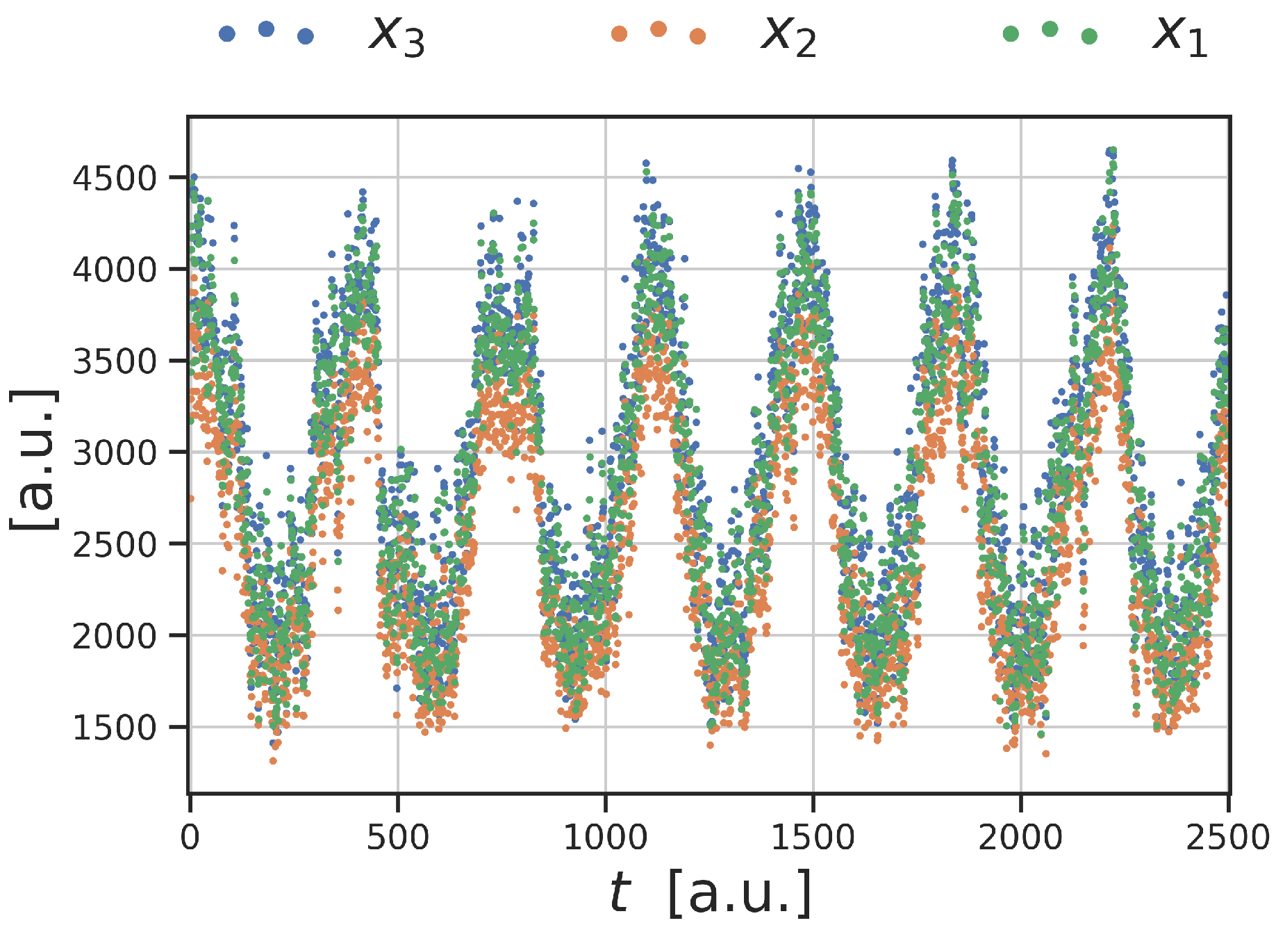
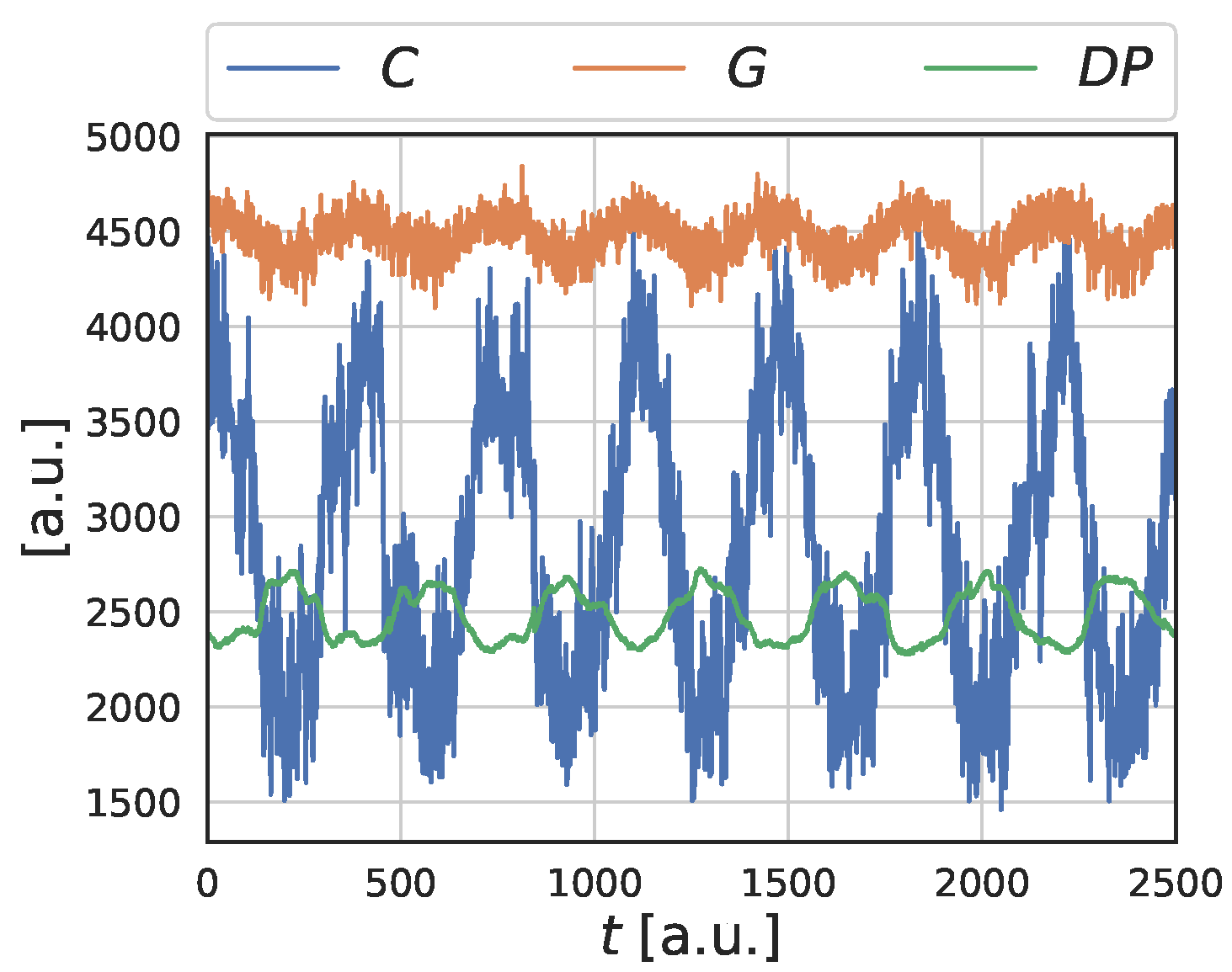
In this analysis, we have decided to use the three highly correlated signals shown in Figure 3. These signals are close to sinusoidal because they were collected during a slug flow: great bubbles of low and high density fluid were alternating [18,59]. We have chosen these data because here global and local anomalies are easily identifiable by visual inspection.
4.1. Fault Types
Measuring instruments can incur many types of fault. Dunia [60] has isolated four elementary faults: the bias, the drift, the precision degradation, and the complete failure fault (Figure 4). Although a general event can be a combination of these faults, we have decided to rely on this classification in order to provide a more robust benchmark.
While bias, complete failure, and precision degradation do not evolve in time, the drift fault has a linear deteriorating behavior. This is why in the following paragraphs we will make different analysis depending on the fault type.
4.2. Synthetic Fault Generation
One of the main challenges in evaluating AD approaches is that tagged data are required, even though typically these are not available. This is the reason why unsupervised approaches are chosen in the first place. In this case study, a number of faults have been added over real MPFM data in order to have a sure evaluation of the effectiveness of the AD4MPFM approach.
The synthetic faults were obtained adding anomalies inside these data, in particular the faults were generated on , the earliest signal (Figure 3 and Figure 4). In order to be consistent between different signals and datasets, the anomaly amplitude is proportional to the median absolute deviation of the anomalous signal.
Given a signal x belonging to the module X and indexed by the discrete time , the bias fault of module X has been obtained in the following way (Figure 4c),
where is the Bernoulli distribution, c is the outlier contamination, and
A has been named anomaly amplitude and takes values in .
Unlike other faults, the drift evolves in time:
where
Together with fault type and anomaly detection models, we vary the following quantities in order to provide an extended evaluation of the AD4MPFM efficiency; contamination, anomaly amplitude, window size , and window overlap .
4.3. Research Questions
In the design of the experiments we have decided to define some guidelines for investigation. To prove the effectiveness of the AD4MPFM approach and to show the effect of different design choices, we have developed various experiments aiming at exposing the impact of each building block of the AD4MPFM pipeline depicted in Figure 2.
With respect to the preprocessing block, we will show in the next section by visual inspection how resulting features do have a discriminative quality.
Regarding the anomaly detection block, as unsupervised AD methods are not widely used in CMS, we will focus our investigation in showing the performance of various methods, the effect of parameter tuning, and the impact on various fault types. In the wide context of Unsupervised Anomaly Detection methods, we will compare six different approaches, namely, CBLOF, HBOS, IF, MAD, MCD, and PCA, that are representative of the four families described in Section 3.2.6. In particular, we have chosen approaches that can be implemented in typical CMS scenarios: this will be discussed in more detail in Section 5. In particular, concerning the static faults, namely, the ones that do not evolve in time (complete failure, bias, and precision degradation), we will try to answer the following questions.
- (a)
- Given an anomaly amplitude, how does the contamination affect the performances of each model?
- (b)
- Given a contamination, how does the anomaly amplitude affect the performances of each model?
- (c)
- In the general case where both the anomaly amplitude and the contamination can vary, which is the model that behaves better?
On the contrary, for the drift case, we will address other questions that will be answered in Section 5.5:
- (i)
- Given a contamination value and some windowing settings, which is the model that performs better along the windows?
- (ii)
- Are there any differences if the contamination changes?
- (iii)
- How is the optimal threshold affected by the contamination?
Later, in Section 5, we will wonder which is the best AD method among the ones shown in Section 3.2.6, given the computational complexity.
Finally, with respect to the Root Cause Analysis block, we will perform analysis by visual inspection that show the effectiveness of the guilty direction procedure.
5. Experimental Results
5.1. Preprocessing
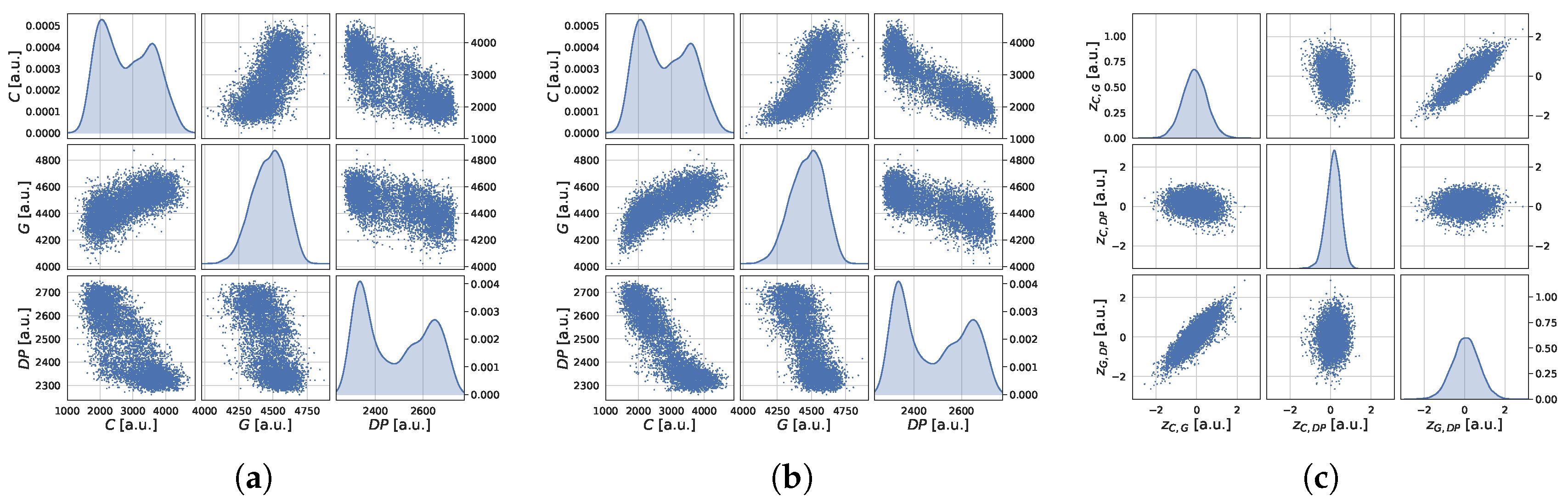
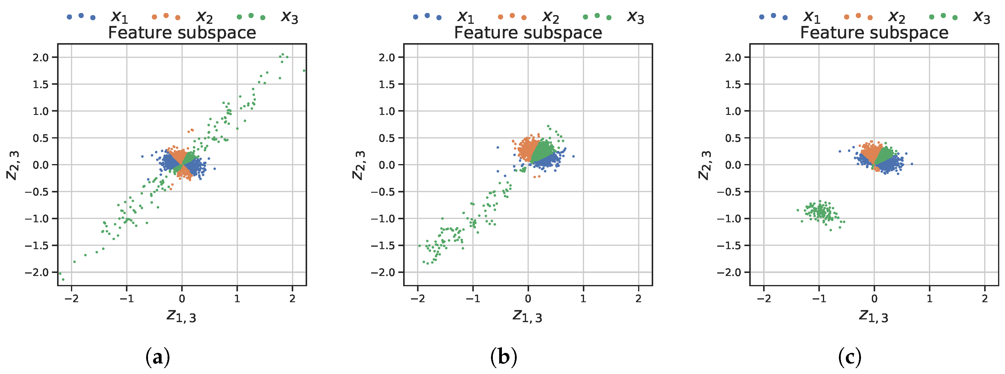
We remark that, in the AD4MPFM pipeline, the goal of the preprocessing block is to decouple the observed dynamics of the underlying process from the behavior of the metrology instrument; in order to demonstrate such capacity, we report in Figure 5 an example of the time series evolution of the MPFM raw data. Moreover, in Figure 6, scatterplot matrices of the same data are reported, by also showing the effect of the preprocessing steps. In particular, in panel (a) of Figure 6, impedance, gamma, and Venturi module measurements are reported. It can be easily appreciated that the two dimensional distributions between two variables are not Gaussian, making it difficult to implement self-diagnosis procedures. In panel (b), showing the data after the alignment step, it can be seen how cross-correlations have been enhanced. Finally, in panel (c), it is evident the benefit of the feature design step: features now exhibit Gaussian distributions that will ease the detection of CMS anomalies as expected.
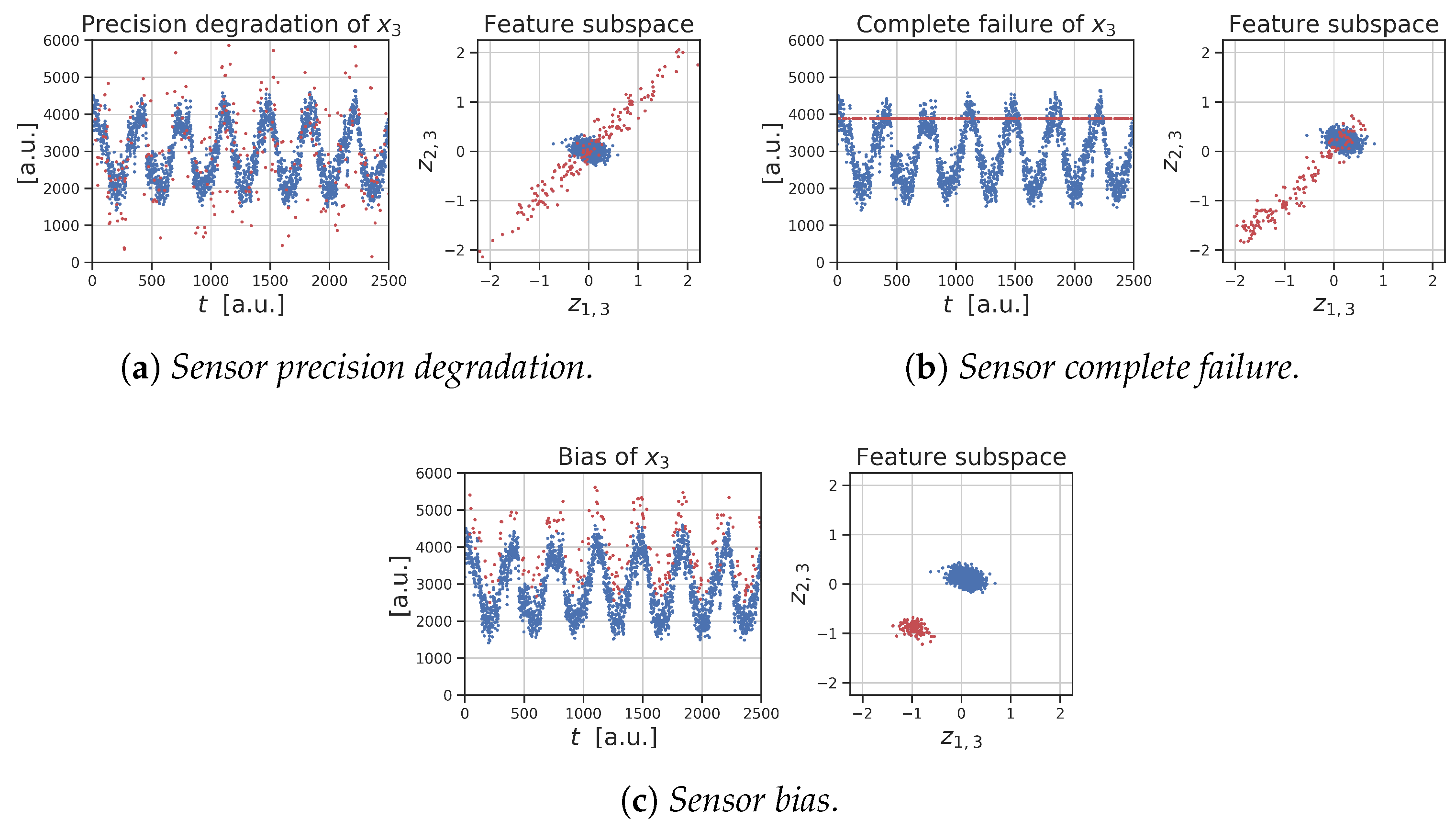
The effectiveness of the proposed preprocessing box can be appreciated even more in the semi-synthetic data reported in Figure 4. The simulated faults are shown on the left panel and the corresponding data, after the feature design process, are shown on the right. The corrupted data are colored in red. It is clear the advantage given by the proposed manipulation: local, global, and context anomalies can be more easily identified. Note that the few corrupted points that cannot be distinguished are the ones were the added noise is almost equal to zero.
While the signals shown in Figure 4 represent only some of the many trends that the flow can develop depending on the operating point, we have seen that the preprocessing block of AD4MPFM is effective in any of the observed conditions: unfortunately, we cannot report here for conciseness other examples, but such effective behavior is demonstrated by the AD results reported in the following experiments that are based on this preprocessing step.
We stress the fact that the preprocessing phase greatly simplifies the task of detecting outliers: instead of monitoring a continuously changing complex signal pattern, the unsupervised AD methods has only to detect the outliers that lie outside the unique central cluster.
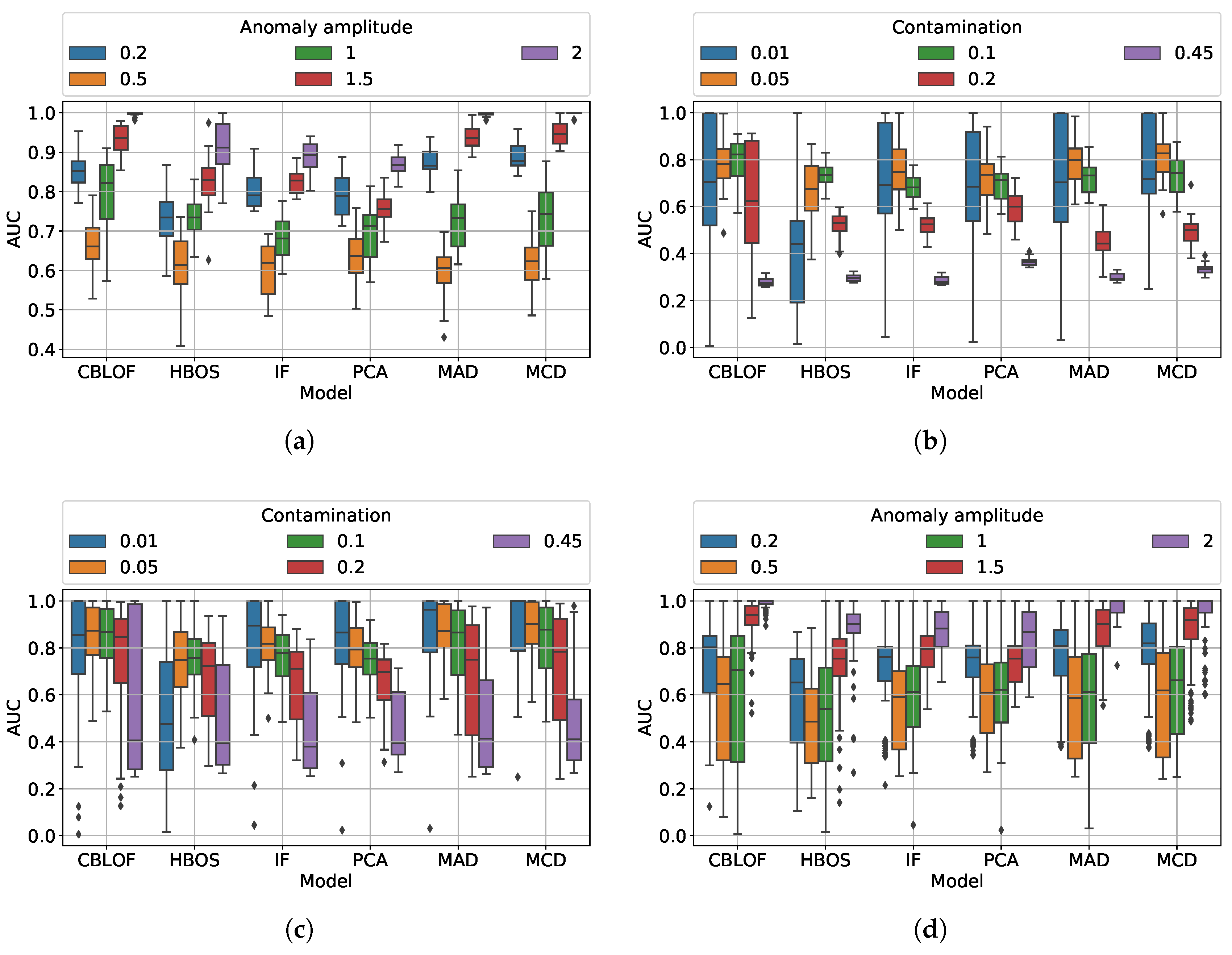
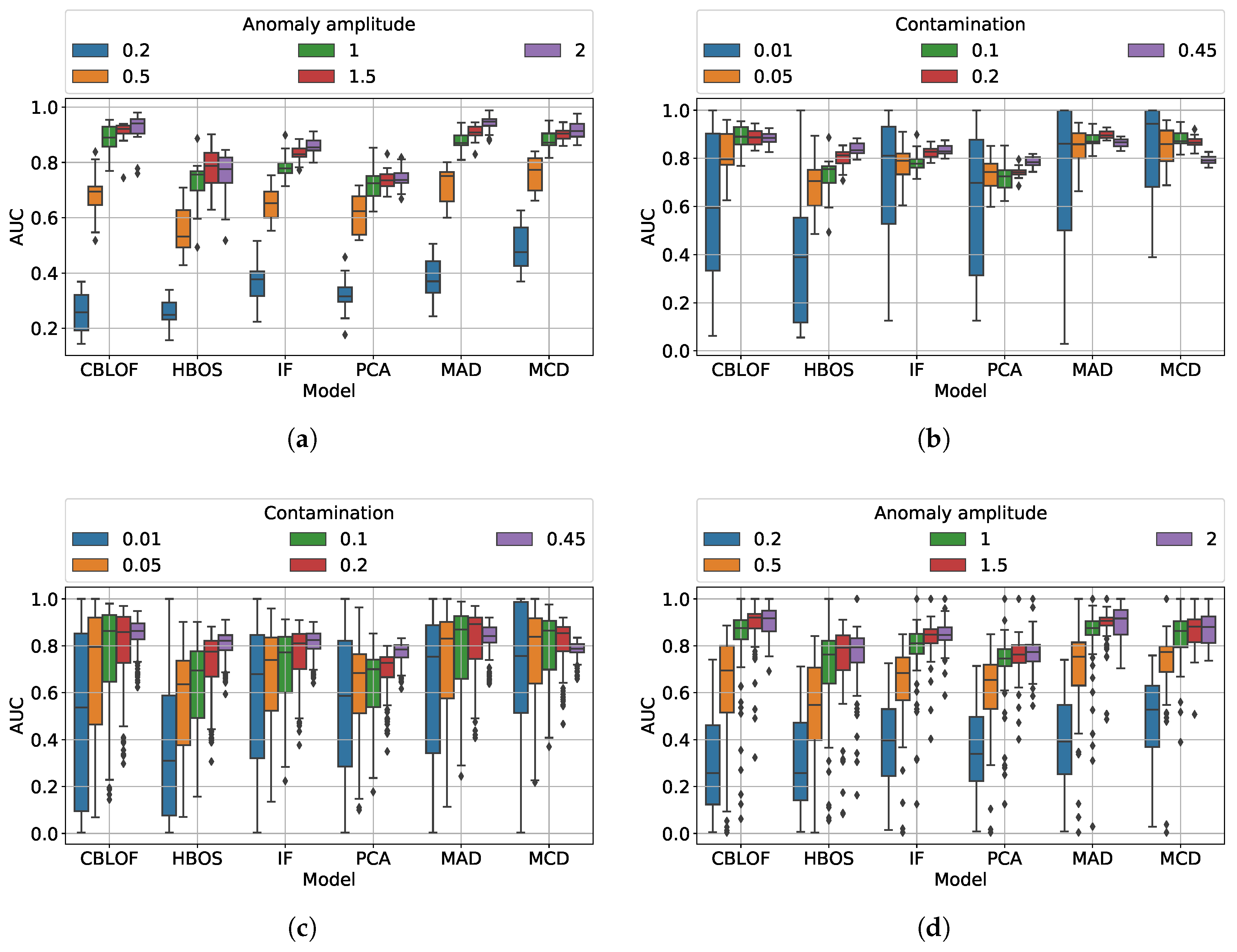
5.2. AD Module: Complete Failure
During a complete failure fault, the anomalous signal keeps a constant trend. An example of feature subspace containing this type of anomalies is shown in Figure 4b. The fault was generated on : the correct samples gather in a central cluster, whereas the anomalous samples distribute on the diagonal. The majority of them can be easily distinguished by the normal cluster, indeed the only anomalies that cannot be detected are those within the normal process dynamics. Beware that the normal cluster width and position can be affected by the normalization phase: if the reference window is seriously corrupted, the reference median and mad can be biased. For this reason, care must be taken on the choice of the scaling references.
5.2.1. Question (a)
Given an anomaly amplitude and for small values of contamination, the best methods seems to be MCD and MAD (Figure 7b). Increasing the contamination, the performances of almost every method get worse: only the CBLOF seems not to be affected by the anomaly concentration. At very high contamination, all the methods have a very low AUC.
5.2.2. Question (b)
Fixing the contamination, the minimum AUC value is obtained for anomaly amplitude between 0.5 and 1. CBLOF performs better, followed by MAD and MCD. PCA is among the worst (Figure 7a).
5.2.3. Question (c)
In the more general case (Figure 7c,d), both the amplitude and the contamination vary. There, CBLOF performs substantially better and has less deteriorating capabilities; it seems not to be robust only at high contamination level.
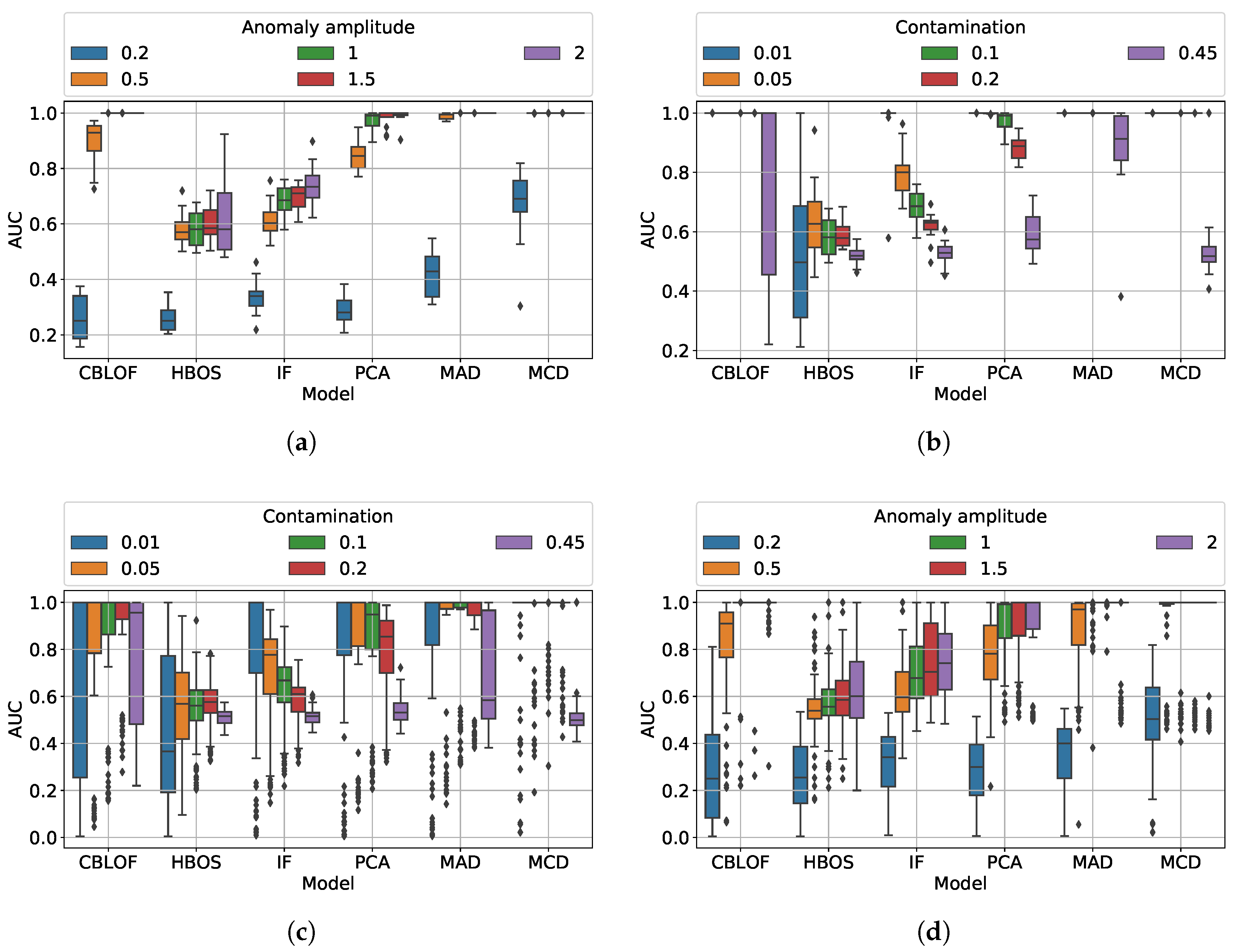
5.3. AD Module: Bias
In the bias fault of Figure 4c, both contextual and global anomalies are present. The surprisingly good ability of the feature design process to distinguish both types of anomalies is shown in the feature subspace. The normal central cluster is still there, but another anomalous cluster is present on the diagonal.
5.3.1. Question (a)
At fixed A, MAD has less deteriorating performances. CBLOF is very good but, as expected it is not robust at high contamination. IF deteriorates as c increases (Figure 8b).
5.3.2. Question (b)
Fixing c it is possible to observe many interesting facts: MCD is able to detect the smallest anomalies. MAD performs well but CBLOF recovers quickly. HBOS and IF perform almost the same way, independently on the anomaly amplitude (Figure 8a).
5.3.3. Question (c)
It is not simple to get conclusions on the general case from Figure 8c,d. MCD works better excluding at high c. CBLOF and MAD outperform the other methods when the anomalies are quite evident.
5.4. AD Module: Precision Degradation
The feature design process distributes the anomalies on an ellipse centered in the normal cluster (Figure 4a). As before, too small anomalies cannot be detected, but it is not important as they are within the normal signal noise. Note that the central cluster is more centered because these anomalies do not bias the reference median and mad.
5.4.1. Question (a)
While MAD and CBLOF have better performance at high c, MCD has the best performance at low contamination level. Increasing the number of outliers, the other methods improve their AUC (Figure 9b).
5.4.2. Question (b)
All but PCA and HBOS increase their AUC with the changing anomaly amplitude. As expected, MCD detects the anomalies much earlier (Figure 9a).
5.4.3. Question (c)
When both the anomaly amplitude and the contamination can change, as the contamination increases, CBLOF loses its advantage and is outperformed by MAD and MCD. When the anomalies are small and few, MCD outperforms the other methods; otherwise, MAD and CBLOF are better (Figure 9c,d).
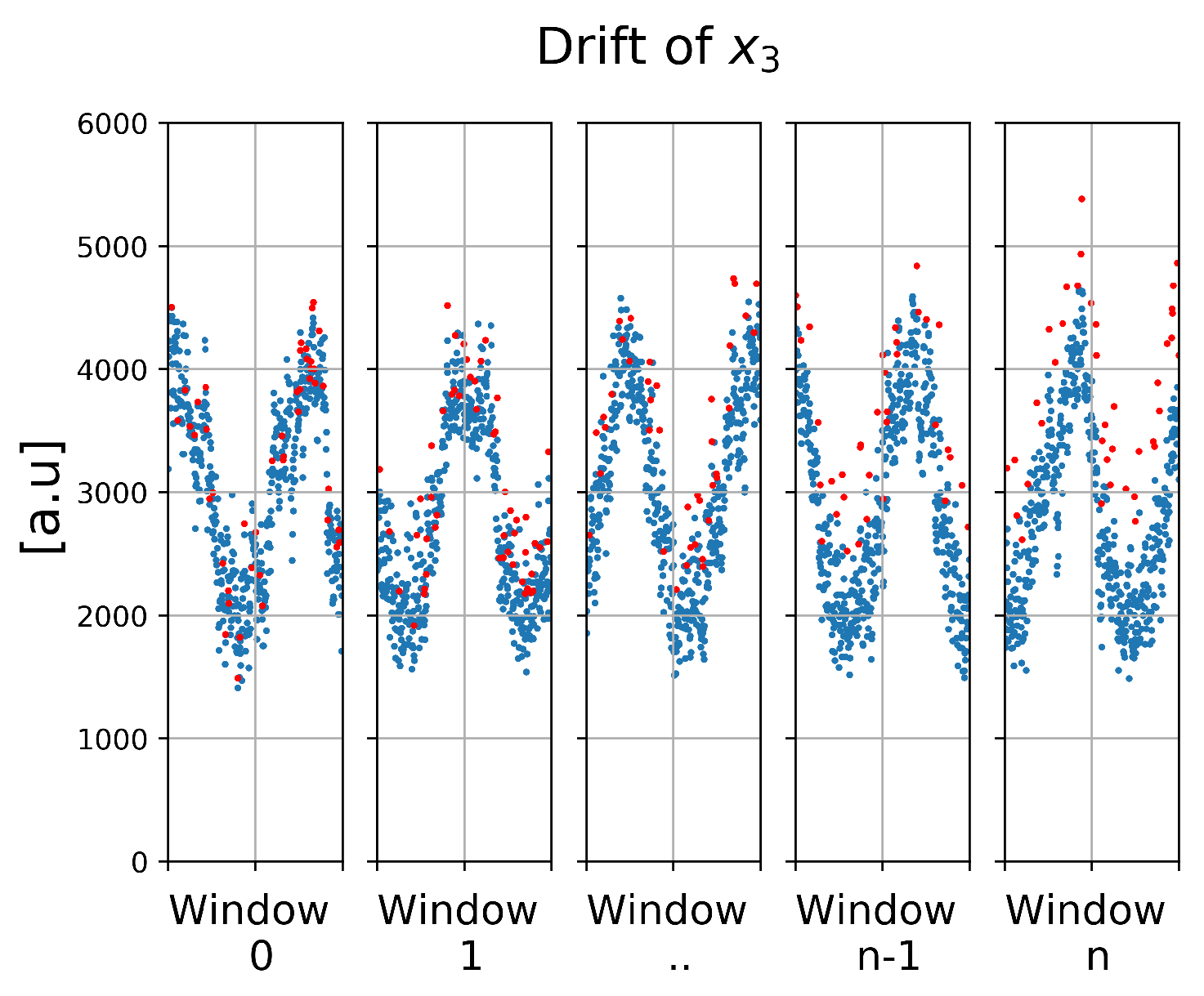
5.5. AD Module: Drift
As drift evolves linearly in time, every window has its own feature subspace (Figure 10). Given a sufficiently small window size, these subspaces can be thought as a sequence of bias faults with increasing anomaly amplitude. In the first window, the anomalous cluster is completely inside the normal cluster, but slowly it comes out.
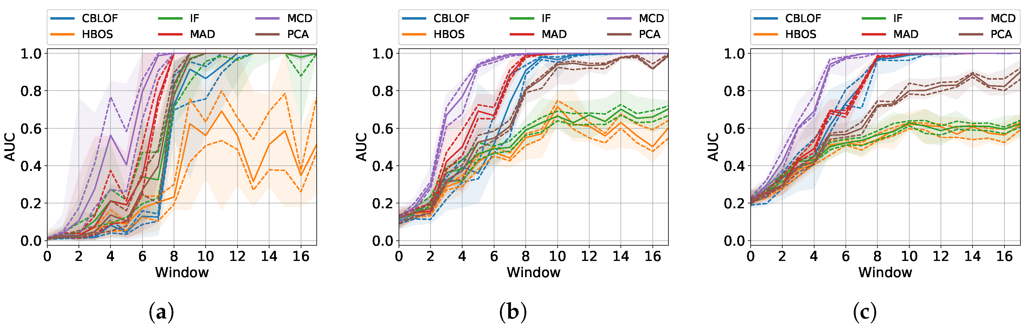
5.5.1. Question (i)
As expected by the previous experiments, MCD detects the fault earlier and MAD has good performance too. In question Section 5.3.2 we have already observed that CBLOF recovers quickly and aligns to MCD and MAD. PCA arrives at good AUC values but too slowly. IF and HBOS saturate quickly at the same low value (Figure 11b).
5.5.2. Question (ii)
Lowering the contamination, the variance of the methods explodes and the AUC score becomes very noisy (Figure 11a). On the contrary, when increasing the number of anomalies, the AUC of the first window improves and the variance reduces.
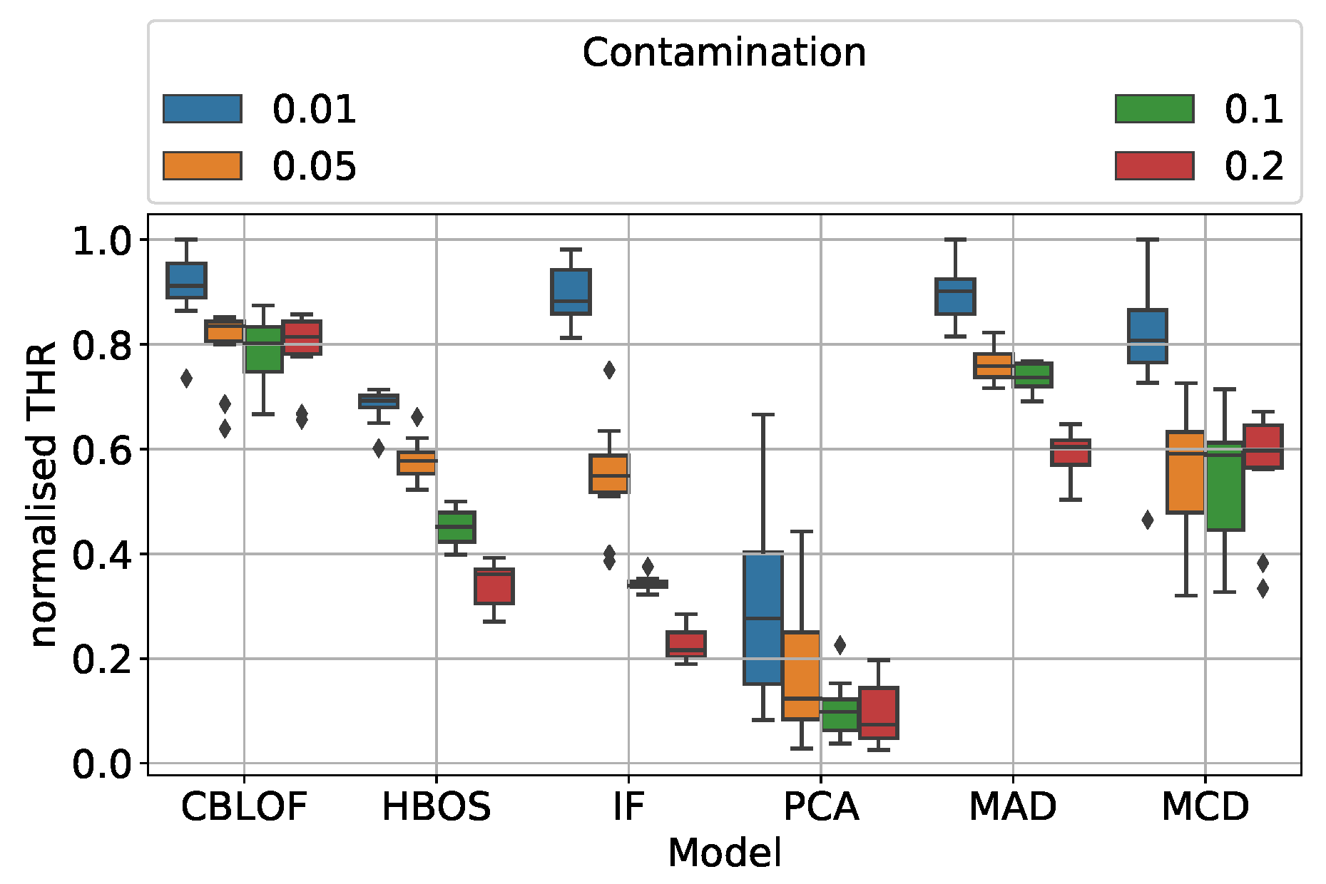
5.5.3. Question (iii)
By optimal threshold we mean the one that maximizes the F1-score. In order to make model and window comparisons, this has to be normalized. Fixing the window, the answer to the question (iii) is quite simple when looking at Figure 12: if the contamination increases, the threshold has to be lowered. However, not all the methods behave in the same way: MCD needs a severe adjustment of the threshold, whereas CBLOF is less affected by the contamination. In this case, PCA performs poorly because it has a huge threshold variation, even inside the contamination classes.
5.6. Root Cause Analysis
The algorithm usually applies the RCA only to the anomalous samples, but in order to understand how this block works we have applied it on every sample. The results are shown in Figure 13. The first fact that can be noticed is the great ability to correctly classify the faulty module; in these examples, the anomalies are assigned to the faulty signal . The second fact is the great simplicity of the method obtained thanks the proposed feature design: the guilty directions are clearly visible inside the central cluster.
5.7. Implementation Discussion
The results obtained on semi-synthetic datasets are promising, as a matter of fact the AD4MPFM algorithm is able to detect with high performances (accordingly to process experts) the generated fault and the faulty module as shown in the previous experiments. The promising results were the basis for proceeding with edge implementation of the AD4MPFM approach in real MPFMs. While the approach has been designed in order to satisfy real-world constrains of CMSs, several aspects should be taken into account before implementation.
Robustness to outlier severity: robustness is a key property for applications where the CMS is placed in remote or “costly” locations. In fact, the MPFM is a typical example, as such CMS is usually placed in harsh and remote sites. In Section 5.2, Section 5.3 and Section 5.4 we have tested many AD algorithms changing the type of fault and studying their robustness to different fault contaminations and anomaly amplitudes. MAD seems to be the one that in general is less affected by the changing fault conditions.
Threshold setting: from the implementation point of view, the optimal threshold must be easy to be set and has to be stable; indeed, on edge applications (especially with installations in remote sites) correcting the threshold could be hardly viable. Studying the drift fault, we have observed how the optimal threshold behaves and which method exhibit the more stable set up. In our context, CBLOF has the most robust threshold.
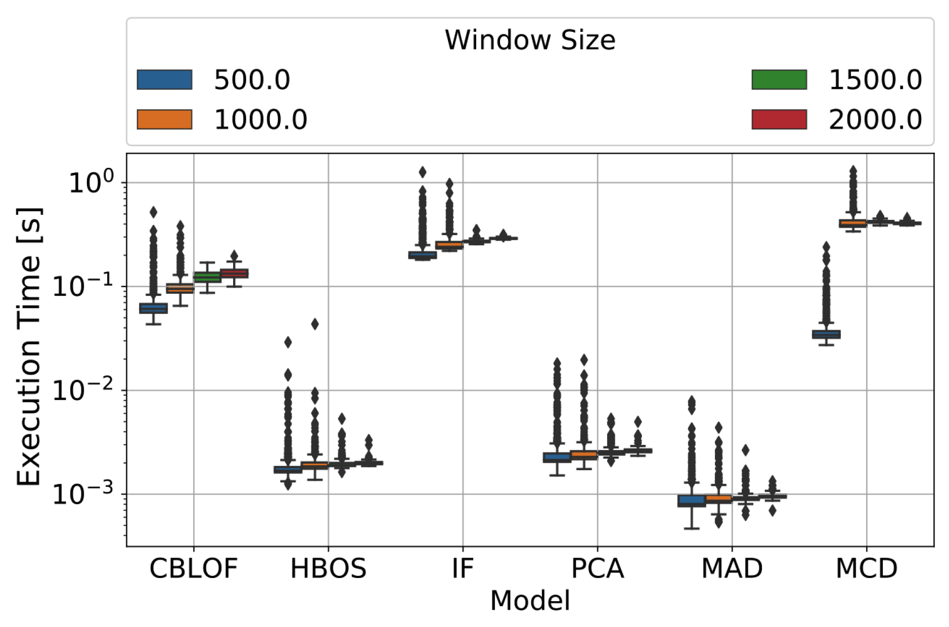
Trade-off between detection abilities and execution time: depending on the application at hand, the choice of the optimal AD method can be done by investigating the trade-off between detection accuracy and execution time. Table 1 and Figure 14 show the mean computational time needed by the AD algorithm to compute the AS for one window. CBLOF, IF, and MCD can be considered heavy methods as they are slower by two degrees of magnitude than MAD, PCA, and HBOS. Unfortunately, MCD was one of the most effective methods, but is the worst compared in terms of execution complexity. Increasing the window amplitude, there is not a significant increase in computational time. As MAD is much faster than the other methods and has good detecting abilities, it can be considered as a good candidate for maximizing the trade-off between the mentioned properties in many application scenarios.
Simplicity of the coding implementation: Simplicity of the coding implementation is a key factor in applications that do not use high level programming languages. MAD is not only the fastest algorithm, but it is also the simplest to be implemented: MAD does not need complex computations and can be easily written in any coding language.
Interpretability: as stated before, interpretability is a key property for monitoring and maintenance-related intelligent tool. For some applications, where interpretability is more relevant than other qualities, MAD is the recommended among the considered AD approaches. MAD threshold is easily interpretable (see Section 3.2.6). Nevertheless, other AD methods can be equipped with interpretability procedure [13]; however, this will require additional complexity that may not be feasible in some application scenarios.
6. Conclusions
In this paper, we have proposed a novel approach for the self-diagnosis and anomaly detection of Multiphase Flow Meters, named AD4MPFM. The approach is specifically designed for handling the typical constrains of complex metrology instruments like the MPFM that are based on multiple sensing modules, time-series streams, and data fusion. The building blocks of AD4MPFM are modern unsupervised anomaly detection techniques and a preprocessing pipeline able to decouple the complex dynamics of the underlying process with the quality of the metrology tool behavior. Moreover, given the importance of interpretability and explainability in monitoring and maintenance contexts, we have equipped AD4MPFM with Root Cause Analysis capabilities, thanks to a so-called guilty direction that points out the module responsible for an anomaly. The main advantage of AD4MPFM is the fact that it does not need historical data to be trained and it is ready for Plug & Play implementations.
The effectiveness of the proposed algorithm has been tested both on semi-synthetic and real datasets. Many types of faults have been simulated, changing the severity of the faulty conditions. As discussed, MPFMs can be very different; therefore, the various desired properties (robustness, accuracy, complexity, etc.) for the self-diagnosis system can vary in order of importance. In this regards, as shown by the experiments reported in this work, the AD4MPFM procedure allows to adopt various design choices in order to make some properties better satisfied than other. As future work, a research direction could be to adopt an ensemble approach on the employed Anomaly Detection methods in order to maintain all the good properties of various unsupervised techniques.
A further remark is that, as shown by the reported experiments, a simple approach like MAD is still very accurate in detection, proving the effectiveness of the preprocessing procedure and on the whole AD4MPFM pipeline.
Additional research investigations will be focused on other two aspects: (i) validation of the proposed approach on new Complex Measuring Systems real case studies, and (ii) the employment of deep learning approaches for anomaly detection that will fit the IoT scenario, where the edge implementation constrain can be relaxed.
Author Contributions
Conceptualization, T.B., E.F., and G.A.S.; investigation, T.B.; resources and validation, E.F.; supervision, G.A.S. All authors have read and agreed to the published version of the manuscript.
Funding
Part of this work was supported by MIUR (Italian Minister for Education) under the initiative “Departments of Excellence” (Law 232/2016). Pietro Fiorentini S.p.A. is gratefully acknowledged for the financial support of this research.
Conflicts of Interest
The authors declare no conflicts of interest.
References
- Weckenmann, A.; Jiang, X.; Sommer, K.D.; Neuschaefer-Rube, U.; Seewig, J.; Shaw, L.; Estler, T. Multisensor data fusion in dimensional metrology. CIRP Ann. 2009, 58, 701–721. [Google Scholar] [CrossRef]
- Hadipour, M.; Derakhshandeh, J.F.; Shiran, M.A. An experimental setup of multi-intelligent control system (MICS) of water management using the Internet of Things (IoT). ISA Trans. 2020, 96, 309–326. [Google Scholar] [CrossRef] [PubMed]
- Jung, D.; Ng, K.Y.; Frisk, E.; Krysander, M. Combining model-based diagnosis and data-driven anomaly classifiers for fault isolation. Control Eng. Pract. 2018, 80, 146–156. [Google Scholar] [CrossRef]
- Ahmad, S.; Lavin, A.; Purdy, S.; Agha, Z. Unsupervised real-time anomaly detection for streaming data. Neurocomputing 2017, 262, 134–147. [Google Scholar] [CrossRef]
- Barbariol, T.; Feltresi, E.; Susto, G.A. Machine Learning approaches for Anomaly Detection in Multiphase Flow Meters. IFAC-PapersOnLine 2019, 52, 212–217. [Google Scholar] [CrossRef]
- Cariño, J.; Delgado-Prieto, M.; Zurita, D.; Picot, A.; Ortega, J.; Romero-Troncoso, R. Incremental novelty detection and fault identification scheme applied to a kinematic chain under non-stationary operation. ISA Trans. 2020, 97, 76–85. [Google Scholar] [CrossRef]
- Chen, Z.; Li, X.; Yang, C.; Peng, T.; Yang, C.; Karimi, H.; Gui, W. A data-driven ground fault detection and isolation method for main circuit in railway electrical traction system. ISA Trans. 2019, 87, 264–271. [Google Scholar] [CrossRef]
- Cheng, Y.; Wang, Z.; Chen, B.; Zhang, W.; Huang, G. An improved complementary ensemble empirical mode decomposition with adaptive noise and its application to rolling element bearing fault diagnosis. ISA Trans. 2019, 91, 218–234. [Google Scholar] [CrossRef]
- Wang-jian, H. Optimal input design for multi UAVs formation anomaly detection. ISA Trans. 2019, 91, 157–165. [Google Scholar] [CrossRef]
- Agrawal, S.; Agrawal, J. Survey on anomaly detection using data mining techniques. Procedia Comput. Sci. 2015, 60, 708–713. [Google Scholar] [CrossRef] [Green Version]
- Theissler, A. Detecting known and unknown faults in automotive systems using ensemble-based anomaly detection. Knowl. Based Syst. 2017, 123, 163–173. [Google Scholar] [CrossRef]
- Meneghetti, L.; Terzi, M.; Del Favero, S.; Susto, G.A.; Cobelli, C. Data-Driven Anomaly Recognition for Unsupervised Model-Free Fault Detection in Artificial Pancreas. IEEE Trans. Control Syst. Technol. 2018, 28, 33–47. [Google Scholar] [CrossRef]
- Carletti, M.; Masiero, C.; Beghi, A.; Susto, G.A. Explainable Machine Learning in Industry 4.0: Evaluating Feature Importance in Anomaly Detection to Enable Root Cause Analysis. In Proceedings of the 2019 IEEE Conference on Systems, Man, and Cybernetics, Bari, Italy, 6–9 October 2019. [Google Scholar]
- Susto, G.A.; Terzi, M.; Masiero, C.; Pampuri, S.; Schirru, A. A Fraud Detection Decision Support System via Human On-Line Behavior Characterization and Machine Learning. In Proceedings of the 2018 First International Conference on Artificial Intelligence for Industries (AI4I), Laguna Hills, CA, USA, 26–28 September 2018; pp. 9–14. [Google Scholar]
- Susto, G.A.; Terzi, M.; Beghi, A. Anomaly detection approaches for semiconductor manufacturing. Procedia Manuf. 2017, 11, 2018–2024. [Google Scholar] [CrossRef]
- Hawkins, D.M. Identification of Outliers; Springer: Berlin/Heidelberg, Germany, 1980; Volume 11. [Google Scholar]
- PietroFiorentini. MPFM FloWatch HS Datasheet. 2011. Available online: https://www.fiorentini.com/ww/en/product/components/mpfm_eng/flowatchhs/ (accessed on 13 October 2019).
- Corneliussen, S.; Couput, J.P.; Dahl, E.; Dykesteen, E.; Frøysa, K.E.; Malde, E.; Moestue, H.; Moksnes, P.O.; Scheers, L.; Tunheim, H. Handbook of Multiphase Flow Metering; Norwegian Society for Oil and Gas Measurement (NFOGM): Oslo, Norway, 2005; Volume 2. [Google Scholar]
- AL-Qutami, T.A.; Ibrahim, R.; Ismail, I.; Ishak, M.A. Virtual multiphase flow metering using diverse neural network ensemble and adaptive simulated annealing. Expert Syst. Appl. 2018, 93, 72–85. [Google Scholar] [CrossRef]
- Andrianov, N. A Machine Learning Approach for Virtual Flow Metering and Forecasting. IFAC-PapersOnLine 2018, 51, 191–196. [Google Scholar] [CrossRef]
- AL-Qutami, T.A.; Ibrahim, R.; Ismail, I.; Ishak, M.A. Radial basis function network to predict gas flow rate in multiphase flow. In Proceedings of the 9th International Conference on Machine Learning and Computing, Vancouver, BC, Canada, 9–14 July 2017; pp. 141–146. [Google Scholar]
- Alger, E.; Kroll, J.; Dzenitis, E.; Montesanti, R.; Hughes, J.; Swisher, M.; Taylor, J.; Segraves, K.; Lord, D.; Reynolds, J.; et al. NIF target assembly metrology methodology and results. Fusion Sci. Technol. 2011, 59, 78–86. [Google Scholar] [CrossRef]
- Franceschini, F.; Galetto, M.; Genta, G. Multivariate control charts for monitoring internal camera parameters in digital photogrammetry for LSDM (Large-Scale Dimensional Metrology) applications. Precision Eng. 2015, 42, 133–142. [Google Scholar] [CrossRef] [Green Version]
- Capriglione, D.; Liguori, C.; Pianese, C.; Pietrosanto, A. On-line sensor fault detection, isolation, and accommodation in automotive engines. IEEE Trans. Instrument. Meas. 2003, 52, 1182–1189. [Google Scholar] [CrossRef]
- Balaban, E.; Saxena, A.; Bansal, P.; Goebel, K.F.; Curran, S. Modeling, detection, and disambiguation of sensor faults for aerospace applications. IEEE Sens. J. 2009, 9, 1907–1917. [Google Scholar] [CrossRef]
- Thennadil, S.N.; Dewar, M.; Herdsman, C.; Nordon, A.; Becker, E. Automated weighted outlier detection technique for multivariate data. Control Eng. Pract. 2018, 70, 40–49. [Google Scholar] [CrossRef] [Green Version]
- Beghi, A.; Cecchinato, L.; Corazzol, C.; Rampazzo, M.; Simmini, F.; Susto, G.A. A one-class svm based tool for machine learning novelty detection in hvac chiller systems. IFAC Proc. Vol. 2014, 47, 1953–1958. [Google Scholar] [CrossRef] [Green Version]
- Araya, D.B.; Grolinger, K.; ElYamany, H.F.; Capretz, M.A.; Bitsuamlak, G. An ensemble learning framework for anomaly detection in building energy consumption. Energy Build. 2017, 144, 191–206. [Google Scholar] [CrossRef]
- Amiruddin, A.A.A.M.; Zabiri, H.; Jeremiah, S.S.; Teh, W.K.; Kamaruddin, B. Valve stiction detection through improved pattern recognition using neural networks. Control Eng. Pract. 2019, 90, 63–84. [Google Scholar] [CrossRef]
- Betta, G.; Pietrosanto, A. Instrument fault detection and isolation: State of the art and new research trends. IEEE Trans. Instrum. Meas. 2000, 49, 100–107. [Google Scholar] [CrossRef]
- Lu, B.; Stuber, J.; Edgar, T.F. Integrated online virtual metrology and fault detection in plasma etch tools. Ind. Eng. Chem. Res. 2013, 53, 5172–5181. [Google Scholar] [CrossRef]
- Ji, H.; He, X.; Shang, J.; Zhou, D. Incipient fault detection with smoothing techniques in statistical process monitoring. Control Eng. Pract. 2017, 62, 11–21. [Google Scholar] [CrossRef]
- Koushanfar, F.; Potkonjak, M.; Sangiovanni-Vincentelli, A. On-line fault detection of sensor measurements. In Proceedings of the SENSORS, Toronto, ON, Canada, 22–24 October 2003; Volume 2, pp. 974–979. [Google Scholar]
- Susto, G.A.; Beghi, A. A virtual metrology system based on least angle regression and statistical clustering. Appl. Stoch. Models Bus. Ind. 2013, 29, 362–376. [Google Scholar] [CrossRef]
- O’Reilly, C.; Gluhak, A.; Imran, M.A.; Rajasegarar, S. Anomaly detection in wireless sensor networks in a non-stationary environment. IEEE Commun. Surv. Tutor. 2014, 16, 1413–1432. [Google Scholar] [CrossRef] [Green Version]
- Yao, Y.; Sharma, A.; Golubchik, L.; Govindan, R. Online anomaly detection for sensor systems: A simple and efficient approach. Perform. Eval. 2010, 67, 1059–1075. [Google Scholar] [CrossRef]
- Corizzo, R.; Ceci, M.; Japkowicz, N. Anomaly detection and repair for accurate predictions in geo-distributed Big Data. Big Data Res. 2019, 16, 18–35. [Google Scholar] [CrossRef]
- Islam, R.U.; Hossain, M.S.; Andersson, K. A novel anomaly detection algorithm for sensor data under uncertainty. Soft Comput. 2018, 22, 1623–1639. [Google Scholar] [CrossRef] [Green Version]
- Susto, G.A.; Cenedese, A.; Terzi, M. Time-series classification methods: Review and applications to power systems data. In Big Data Application in Power Systems; Elsevier: Amsterdam, The Netherlands, 2018; pp. 179–220. [Google Scholar]
- Susto, G.A.; Schirru, A.; Pampuri, S.; Beghi, A.; De Nicolao, G. A hidden-gamma model-based filtering and prediction approach for monotonic health factors in manufacturing. Control Eng. Pract. 2018, 74, 84–94. [Google Scholar] [CrossRef]
- Ahmad, S.; Purdy, S. Real-time anomaly detection for streaming analytics. arXiv 2016, arXiv:1607.02480. [Google Scholar]
- Hollingsworth, K.; Rouse, K.; Cho, J.; Harris, A.; Sartipi, M.; Sozer, S.; Enevoldson, B. Energy Anomaly Detection with Forecasting and Deep Learning. In Proceedings of the 2018 IEEE International Conference on Big Data (Big Data), Seattle, WA, USA, 10–13 December 2018; pp. 4921–4925. [Google Scholar]
- Ryan, S.; Corizzo, R.; Kiringa, I.; Japkowicz, N. Pattern and Anomaly Localization in Complex and Dynamic Data. In Proceedings of the 2019 18th IEEE International Conference On Machine Learning And Applications (ICMLA), Boca Raton, FL, USA, 16–19 December 2019; pp. 1756–1763. [Google Scholar]
- Hochenbaum, J.; Vallis, O.S.; Kejariwal, A. Automatic anomaly detection in the cloud via statistical learning. arXiv 2017, arXiv:1704.07706. [Google Scholar]
- Kuo, Y.H.; Li, Z.; Kifer, D. Detecting Outliers in Data with Correlated Measures. In Proceedings of the 27th ACM International Conference on Information and Knowledge Management, Turin, Italy, 22–26 October 2018; pp. 287–296. [Google Scholar]
- Idé, T.; Papadimitriou, S.; Vlachos, M. Computing correlation anomaly scores using stochastic nearest neighbors. In Proceedings of the Seventh IEEE international conference on data mining (ICDM 2007), Omaha, NE, USA, 28–31 October 2007; pp. 523–528. [Google Scholar]
- Gautam, S.; Tamboli, P.K.; Roy, K.; Patankar, V.H.; Duttagupta, S.P. Sensors incipient fault detection and isolation of nuclear power plant using extended Kalman filter and Kullback–Leibler divergence. ISA Trans. 2019, 92, 180–190. [Google Scholar] [CrossRef]
- Azaria, M.; Hertz, D. Time delay estimation by generalized cross correlation methods. IEEE Trans. Acoust. Speech Signal Process. 1984, 32, 280–285. [Google Scholar] [CrossRef]
- Keogh, E.; Ratanamahatana, C.A. Exact indexing of dynamic time warping. Knowl. Inf. Syst. 2005, 7, 358–386. [Google Scholar] [CrossRef]
- Aggarwal, C.C. Outlier analysis. In Data Mining; Springer: Berlin/Heidelberg, Germany, 2015; pp. 237–263. [Google Scholar]
- Deng, X.; Wang, L. Modified kernel principal component analysis using double-weighted local outlier factor and its application to nonlinear process monitoring. ISA Trans. 2018, 72, 218–228. [Google Scholar] [CrossRef]
- He, Z.; Xu, X.; Deng, S. Discovering cluster-based local outliers. Pattern Recognit. Lett. 2003, 24, 1641–1650. [Google Scholar] [CrossRef]
- Goldstein, M.; Dengel, A. Histogram-based outlier score (hbos): A fast unsupervised anomaly detection algorithm. In Proceedings of the KI-2012: Poster and Demo Track, Saarbrucken, Germany, 24–27 September 2012; pp. 59–63. [Google Scholar]
- Shyu, M.L.; Chen, S.C.; Sarinnapakorn, K.; Chang, L. A Novel Anomaly Detection Scheme Based on Principal Component Classifier; Technical Report; University of Miami: Coral Gables, FL, USA, 2003. [Google Scholar]
- Hubert, M.; Debruyne, M.; Rousseeuw, P.J. Minimum covariance determinant and extensions. Wiley Interdiscip. Rev. Comput. Stat. 2018, 10, e1421. [Google Scholar] [CrossRef] [Green Version]
- Liu, F.T.; Ting, K.M.; Zhou, Z.H. Isolation-based anomaly detection. ACM Trans. Knowl. Discov. Data (TKDD) 2012, 6, 3. [Google Scholar] [CrossRef]
- Rousseeuw, P.J.; Croux, C. Alternatives to the median absolute deviation. J. Am. Stat. Assoc. 1993, 88, 1273–1283. [Google Scholar] [CrossRef]
- Saito, T.; Rehmsmeier, M. The precision-recall plot is more informative than the ROC plot when evaluating binary classifiers on imbalanced datasets. PLoS ONE 2015, 10, e0118432. [Google Scholar] [CrossRef] [Green Version]
- Brennen, C.E.; Brennen, C.E. Fundamentals of Multiphase Flow; Cambridge University Press: Cambridge, UK, 2005. [Google Scholar]
- Dunia, R.; Qin, S.J.; Edgar, T.F.; McAvoy, T.J. Identification of faulty sensors using principal component analysis. AIChE J. 1996, 42, 2797–2812. [Google Scholar] [CrossRef]
- Zhao, Y.; Nasrullah, Z.; Li, Z. PyOD: A python toolbox for scalable outlier detection. J. Mach. Learn. Res. 2019, 20, 1–7. [Google Scholar]
Figure 1.
Example of a modular topside Multiphase Flow Meter (MPFM). The vertical pipe is the Venturi tube, where the mixture coming from the well flows. The horizontal tube is the densitometer, while the pressure, impedance and temperature probes are hidden inside the pipe.
Figure 1.
Example of a modular topside Multiphase Flow Meter (MPFM). The vertical pipe is the Venturi tube, where the mixture coming from the well flows. The horizontal tube is the densitometer, while the pressure, impedance and temperature probes are hidden inside the pipe.

Figure 2.
AD4MPFM: Flowchart of the proposed algorithm for anomaly detection of Multiphase Flow Meters.
Figure 2.
AD4MPFM: Flowchart of the proposed algorithm for anomaly detection of Multiphase Flow Meters.

Figure 3.
Small interval of the three employed signals. Their high correlation is used by the method to detect possible faults.
Figure 3.
Small interval of the three employed signals. Their high correlation is used by the method to detect possible faults.

Figure 4.
(sx) Synthetic anomalous signal obtained starting from the real signal of Figure 3. Contamination 10%, anomaly amplitude 1. (dx) Corresponding feature subspace. Synthetic anomalies are red colored. We highlight the effectiveness of the preprocessing block of AD4MPFM that makes anomalous samples lie on the subspace diagonal.

Figure 5.
Real Data: raw signal example. Signals from different modules are not aligned in time and have different scales.
Figure 5.
Real Data: raw signal example. Signals from different modules are not aligned in time and have different scales.

Figure 6.
Real data: physics dynamics and meter behavior decoupling of signals shown in Figure 5. (a) Scatter plot of the signals. They can draw very different patterns depending on their value, misalignment and correlation. (b) Signal alignment. It always improves the correlation between the signals. (c) Data after the process filtering. The measured dynamics is filtered and only the instrumentation behavior is shown.

Figure 7.
Complete failure. (a) Fixed contamination 10%. The anomaly amplitude varies. (b) Fixed anomaly amplitude 1. The contamination varies. (c) General case, where both the anomaly amplitude and the contamination vary. Contamination view. (d) General case, where both the anomaly amplitude and the contamination vary. Anomaly amplitude view.

Figure 8.
Bias. (a) Fixed contamination 10%. The anomaly amplitude varies. (b) Fixed anomaly amplitude 1. The contamination varies. (c) General case, where both the anomaly amplitude and the contamination vary. Contamination view. (d) General case, where both the anomaly amplitude and the contamination vary. Anomaly amplitude view.

Figure 9.
Precision degradation. (a) Fixed contamination %10. The anomaly amplitude varies. (b) Fixed anomaly amplitude 1. The contamination varies. (c) General case, where both the anomaly amplitude and the contamination vary. Contamination view. (d) General case, where both the anomaly amplitude and the contamination vary. Anomaly amplitude view.

Figure 10.
Sensor drift. The signal has been windowed in n segments in order to highlight the n different anomaly settings. The representation of the data in the feature subspace is not reported here for conciseness, but for obvious reasons it would be similar to the one reported in panel (c) of Figure 4 with various anomaly amplitudes.

Figure 11.
Drift fault: evolution of the area under the curve (AUC) score along the windows. The performances are strongly sensitive to the outliers contamination. The shade extends from the minimum and maximum values of the data, the dashed lines represents the first and third quartiles, while the solid line is the median (second quartile). (a) 1% of contamination. (b) 10% of contamination. (c) 20% of contamination.

Figure 12.
Normalized F1-max-threshold of the last window. Not every method starts from the max threshold because the normalization has been done on all the windows and sometimes a larger threshold has been used in previous windows.
Figure 12.
Normalized F1-max-threshold of the last window. Not every method starts from the max threshold because the normalization has been done on all the windows and sometimes a larger threshold has been used in previous windows.

Figure 13.
Root Cause Analysis: The samples in the feature subspace are colored by guilty index. It is clear the simplicity and the effectiveness of the proposed method. (a) Precision degradation fault. (b) Complete failure fault. (c) Bias fault.
Figure 13.
Root Cause Analysis: The samples in the feature subspace are colored by guilty index. It is clear the simplicity and the effectiveness of the proposed method. (a) Precision degradation fault. (b) Complete failure fault. (c) Bias fault.

Figure 14.
Plot of the computational time employed by each unsupervised method, for different window sizes. Two groups can be distinguished: CBLOF, IF, and MCD are very slow, whereas HBOS, PCA, and MAD are very fast methods.
Figure 14.
Plot of the computational time employed by each unsupervised method, for different window sizes. Two groups can be distinguished: CBLOF, IF, and MCD are very slow, whereas HBOS, PCA, and MAD are very fast methods.


Table 1.
Execution Time [ms]. The algorithm has been designed to work on a Zynq-7000 ARM cortex A9, but the execution time of the algorithms was measured on a 2.7 GHz Intel Core 5 Processor and refers to the PyOD implementation available in [61].
Table 1.
Execution Time [ms]. The algorithm has been designed to work on a Zynq-7000 ARM cortex A9, but the execution time of the algorithms was measured on a 2.7 GHz Intel Core 5 Processor and refers to the PyOD implementation available in [61].
| Model/Window Size | 500 | 1000 | 1500 | 2000 |
|---|---|---|---|---|
| CBLOF | 60.9 | 96.3 | 121.2 | 140.7 |
| HBOS | 1.7 | 1.9 | 1.9 | 2.0 |
| IF | 195.0 | 243.9 | 270.9 | 297.8 |
| MAD | 0.8 | 0.9 | 0.9 | 1.0 |
| MCD | 33.9 | 399.2 | 417.2 | 422.0 |
| PCA | 2.1 | 2.3 | 2.5 | 2.6 |
© 2020 by the authors. Licensee MDPI, Basel, Switzerland. This article is an open access article distributed under the terms and conditions of the Creative Commons Attribution (CC BY) license (http://creativecommons.org/licenses/by/4.0/).
Share and Cite
MDPI and ACS Style
Barbariol, T.; Feltresi, E.; Susto, G.A. Self-Diagnosis of Multiphase Flow Meters through Machine Learning-Based Anomaly Detection. Energies 2020, 13, 3136. https://doi.org/10.3390/en13123136
AMA Style
Barbariol T, Feltresi E, Susto GA. Self-Diagnosis of Multiphase Flow Meters through Machine Learning-Based Anomaly Detection. Energies. 2020; 13(12):3136. https://doi.org/10.3390/en13123136
Chicago/Turabian StyleBarbariol, Tommaso, Enrico Feltresi, and Gian Antonio Susto. 2020. "Self-Diagnosis of Multiphase Flow Meters through Machine Learning-Based Anomaly Detection" Energies 13, no. 12: 3136. https://doi.org/10.3390/en13123136
Note that from the first issue of 2016, this journal uses article numbers instead of page numbers. See further details here.