Self-Learning Data-Based Models as Basis of a Universally Applicable Energy Management System
by
 , , , ,
Malin Lachmann
1,† ,
,
Jaime Maldonado
2,†,
Wiebke Bergmann
1,3,†,
Francesca Jung
1,†,
Markus Weber
1 and
Christof Büskens
1,* 1
Center for Industrial Mathematics, University of Bremen, Bibliothekstr. 5, 28359 Bremen, Germany
2
Cognitive Neuroinformatics, University of Bremen, Enrique-Schmidt-Straße 5, 28359 Bremen, Germany
3
Steinbeis Innovation Center for Optimization and Control, Schmalenbecker Str. 33, 28879 Grasberg, Germany
*
Author to whom correspondence should be addressed.
†
These authors contributed equally to this work.
Energies 2020, 13(8), 2084; https://doi.org/10.3390/en13082084
Submission received: 20 March 2020
/
Revised: 15 April 2020
/
Accepted: 16 April 2020
/
Published: 21 April 2020
(This article belongs to the Special Issue Applications of Artificial Intelligence in Renewable Energy)
Abstract
:In the transfer from fossil fuels to renewable energies, grid operators, companies and farms develop an increasing interest in smart energy management systems which can reduce their energy expenses. This requires sufficiently detailed models of the underlying components and forecasts of generation and consumption over future time horizons. In this work, it is investigated via a real-world case study how data-based methods based on regression and clustering can be applied to this task, such that potentially extensive effort for physical modeling can be decreased. Models and automated update mechanisms are derived from measurement data for a photovoltaic plant, a heat pump, a battery storage, and a washing machine. A smart energy system is realized in a real household to exploit the resulting models for minimizing energy expenses via optimization of self-consumption. Experimental data are presented that illustrate the models’ performance in the real-world system. The study concludes that it is possible to build a smart adaptive forecast-based energy management system without expert knowledge of detailed physics of system components, but special care must be taken in several aspects of system design to avoid undesired effects which decrease the overall system performance.
1. Introduction
To successfully master the energy transition away from fossil fuels towards renewable energies, many different problems have to be solved [1]. The first step of building new renewable energy plants has been realized very successfully in Germany [2]. However, now the huge amount of energy generated by offshore wind plants in the north of Germany has to be distributed to the entire country. The plans to build new high-voltage transmission lines have resulted in a decreasing acceptance in the population [3]. Therefore, alternative solutions have to be found.
The need for grid expansion can be reduced if energy is produced in the same location where a demand exists. Many companies, farms, and households have taken advantage of the German renewable energy act (EEG) [4], which has encouraged the installation of small to medium sized renewable energy sources on the low and medium voltage level since the year 2000. Since grid parity was reached in Germany a few years ago due to rising energy prices [5], it can be financially beneficial to exploit these installations by increasing self-consumption, i.e., maximizing the amount of locally produced energy that is directly used.
However, to perform such a task in an automated way, smart energy systems are needed which are able to determine and execute optimal operation strategies by rescheduling controllable loads and control of storage devices in accordance with the expected energy production profile. In simple system setups such as integrated PV-storage systems, relay-based self-consumption maximization strategies might suffice and are commonly found in practice [6]. For more complex system setups with several controllable devices, in many cases, more advanced optimization strategies are proposed, which require sufficiently detailed models of system components [7]. In the case of a large office building, a farm, or an industrial premise, loads and devices exhibiting very specific or complex consumption behaviors might prohibit the usage of advanced optimization methods due to the effort of deriving and implementing the necessary white or gray box models. This situation was reported by Žáčeková et al. [8] and Sturzenegger et al. [9] for the usage of model predictive control (MPC) in the minimization of the energy demand of office buildings. Furthermore, the application of forecast methods for the expected power generation is investigated in several studies, indicating financial benefits for a smart energy system or its integration into the overall power system (e.g., [6,10,11]). If these benefits are to be exploited in a smart energy system, forecast models for volatile generation and consumption must also be developed, increasing the initial modeling effort even further.
In the literature, there are basically two superordinate modeling approaches: physical models and data-based models. In the physics-based approach, the physical background of the devices is analyzed and its operation is described by model equations. In contrast, data-based models learn the underlying mapping between input and output variables from recorded data during a training horizon making only general assumptions about the model. While physics-based models require knowledge about the underlying physics which can be very complex, data-based models often require many data and highly depend on the quality and completeness of the data.
Data-based modeling techniques can be classified into statistical and artificial intelligence (AI) techniques [12]. Statistical techniques, also referred to as parametric methods, include linear regression models, autoregressive and moving average (ARMA) models, and exponential smoothing models [12,13]. On the other hand, AI techniques include artificial neural networks (ANNs), fuzzy regression models, support vector machines (SVMs), and gradient boosting machines [12,13]. These approaches are not restricted to one functionality and can be applied to model energy generation, storage or consumption, as shown in the following examples. In [14], forecasts for energy generation are made based on regression methods. In [15], a neural network is applied to estimate the power generated by a wind turbine. In [16], an adaptive neuro-fuzzy inference system is used to forecast power generation of wind plants. In [17], photovoltaic plants are modeled focusing on numerical weather prediction models. Examples for models of energy storages are found in [18,19,20], where the state of charge of a battery is modeled by means of neural networks and other learning approaches.
In the case of statistical techniques, a model of power consumption is constructed by examining qualitative relationships between load and load-affecting factors, which are estimated from historical data [13]. Statistical and AI techniques are regarded as data-based methods, since they rely on the availability of training datasets to establish input–output relationships and to train models. Regardless of the popularity of some techniques, there is no consensus over which particular forecasting model or method to prefer [21].
Recent studies have explicitly exploited the advantage of incorporating data-based modeling techniques directly into optimal energy management methods. In [22], an MPC-like optimization approach based on specially structured data-driven models is proposed for energy management of buildings. It is shown by a simulation study that the result is still comparable to that of a regular MPC approach, but the initial modeling effort can be reduced significantly. In [23], a data-driven demand-side energy management approach is proposed and validated successfully via simulation on real-world data.
This paper presents the results of an integrated real-world case study, reporting beneficial as well as disadvantageous effects of incorporating exclusively data-based models for storages, loads, and generation, including automated update mechanisms in some cases, into a smart energy system. The special contribution of this paper is the documentation of a complete modeling workflow, starting from only historical data through the identification of initial models, up to the discussion of the effects that these models have caused in a fully functional real-world smart energy system, offering valuable insights for the transfer of data-based models into real-world applications.
In detail, clustering and regression are applied as data-based approaches for modeling energy consumption and generation during the design and implementation phases of a forecast-based smart energy management system. The system is applied for the optimization of self-consumption in a real-world estate in a rural area, which includes two service buildings and a four-person household. The underlying scheduling approach of the system was originally introduced in [24] and is chosen because it proved applicable in cases where insight into internal structures of models or derivative information is available only to a limited degree. It is a reactive scheduling routine, i.e., it is based on updating a nominal schedule by frequent recalculation and refinement in a rolling horizon setup [25]. The models considered comprise the forecasting of the power generation of a PV plant, demand of a washing machine and a heat pump device, and predicting the dynamic behavior of the heat pump’s internal temperatures and a battery storage’s state of charge.
Considering the individual models, good results are obtained in terms of a root-mean-square-error measure between model prediction and ground truth on historical data. The experimental results indicate that the overall approach, i.e., a reactive scheduling method incorporating data-based models, has the potential for improving the running energy cost of a given system. Concrete examples are pointed out where properties of the scheduling approach or uncertainties of the models significantly influence the overall result of the scheduling. The relevant uncertainties can be categorized into
- inaccuracies introduced by human interaction;
- volatile forecasts;
- inaccuracies introduced by shortcomings of the training data; and
- physical factors that are not modeled.
While the first two categories are naturally expected in a forecast-based approach, the latter two categories are identified as potential difficulties of a purely data-based approach to modeling when additional information about physical context is not available. Especially the application of models trained on data from uncontrolled (open-loop) operation in a closed-loop setup introduces forecast errors which are not apparent from the error values against ground truth obtained during training.
In Section 2, the requirements for a smart energy management system are formulated and the real-world testing environment is introduced, including information about the measurement system, data processing, and controlled devices. Then, a detailed explanation of the modeling methods used is given in Section 3 including results for each specific device. An introduction to the smart energy system design and formulations of the underlying optimization problems are given in Section 4. In addition to the results in each part of Section 3, experimental results of the optimization are shown in Section 5. A summarizing discussion and a final conclusion in Section 6 complete the paper.
2. Problem Statement
2.1. Requirements for the Integration of Data-Based Models in the Smart Energy Management System
In the experimental setup adopted to investigate the real-world behavior of the data-based models, a forecast-based reactive scheduling approach is used for the optimization of energy cost. The concept is illustrated in Figure 1. It accounts for uncertainty of power forecasts by regular recalculation and is, for the same reason, robust against general modeling inaccuracies and time varying model properties. Forecasts over a future time horizon are computed by evaluating the data-based models on measurements from the overall system (e.g., the household) and external information (e.g., future weather conditions). These forecasts are used as input to an optimization procedure, i.e., a scheduling algorithm, which determines the control signals that are applied to the system over a future time horizon. This is repeated in every control step (rolling horizon), such that controls are updated frequently based on newly available data. The determined controls are communicated to the actuators of the system via a real-time control layer.
The operation of the local energy system with renewable generation, shiftable loads, and energy storages is influenced via demand scheduling and storage management. Constraints such as temperatures of a cooling device, time constraints for a cleaning system, and limitations of states of charge and control signals of battery storages have to be satisfied by the final control strategy. To calculate it for future time horizons, the expected power flow among generators, storages, and loads has to be forecasted. In summary, the following tasks have to be solved:
- Create device models to map input variables (e.g., control signals or weather forecast data) to time series of generated and consumed power and constrained variables (e.g., temperatures and states of charge).
- Compute forecasts for a given prediction horizon by application of the models.
- Calculate optimal control strategies (schedules) for all controllable devices that take all constraints into account and minimize expenses for energy over a given time horizon.
The chosen data-based modeling approaches should furthermore obey two superordinate objectives: (1) The modeling approaches should be very general, and they should be suited for automated re-training and efficient updates when new data become available. Learning models automatically from given data instead of manually developing individual physical models would result in a highly independent and generalizable modeling approach. This allows the efficient addition of new devices as well as an efficient transfer to other sites (e.g., to other company). (2) Given an appropriate update mechanism, the models are adaptive to changes in the external conditions, e.g., in the case of wearout or changes in usage duration, work load, or weather conditions.
2.2. Model Design and Application Approach
The overall workflow of the data-based modeling approach presented in this paper is shown in Figure 2. All data were recorded at a real-world testing environment which is located on an estate in a rural area in Lower Saxony, Germany. The estate is referred to as demonstration site in the following.
In an initial phase (Figure 2a), training data for all the generation plants and power consumers were acquired from the demonstration site via an automated measurement system (see Section 2.3) over several months. The system collects smart meter data, temperature values, weather measurements, weather forecasts, and control signals. Detailed explanations are given in Section 2.4. When sufficient data were available, the selection of a modeling method and the model training were conducted offline in order to obtain an initial model for each relevant device. The main appliances chosen for modeling were a photovoltaic plant, as volatile renewable energy source, and a washing machine, a heat pump, and battery storage, as controllable loads or storages (see Table 1 for further details). During the first phase, started in October 2016, only the battery storage was actually controlled and thus its control signals recorded. Binary controls of washing machine and heat pump were reconstructed under the simplifying assumption that an active power demand is present if and only if a control value of 1 is present during the corresponding timestamp.
Once model structures and initial parameterizations were available, the models were integrated in the smart energy system, which, after that, was able to actively control the live operation of the demonstration site. This is considered as second phase of the workflow (Figure 2b). In this phase, the models produce the forecasts needed for the computation of control schedules and model parameters can be updated. The underlying database is now continuously updated with recent measurements and weather forecast data. Instead of historical control signals, suggestions made by the schedule computation during the optimization process are applied as inputs. Furthermore, the model parameters are automatically updated every 24 h based on new data that have become available since the last update. The installation of the full smart energy system, i.e., the start of Phase 2, took place in the beginning of 2019.
2.3. Demonstration Site System Setup
An overview of the system setup at the demonstration site is shown in Figure 3. The four-person household, utilities in service buildings, and several appliances for the yard cause an uncontrolled basic power demand. The local system has one coupling point to the public low voltage distribution grid and is always grid-connected. An overview of the characteristic properties of the main appliances relevant for modeling and optimization, namely the photovoltaic plant, washing machine, heat pump, and battery storage, is given in Table 1.
The described setup is built for self-consumption operation in accordance with the German renewable energy act [26]. It regulates the conditions under which generated surplus energy by renewable sources, i.e., the amount of energy which cannot be self-consumed directly, can be sold and exported to the public grid. In the presented case, surplus energy by the photovoltaic plant can be sold, as long as the export of energy discharged from the battery storage is prevented. This is achieved by monitoring the power flow at the grid coupling point and immediately stopping the discharge of the battery storage as soon as an export is detected.
The washing machine and the heat pump were chosen for controlled operation because they are, in this specific household, among the appliances with the highest nominal power which are frequently used, but also shiftable in time without affecting the inhabitants’ comfort. Furthermore, their integration into the control system is straightforward: the heat pump is delivered with an SG-ready interface by design, and the washing machine is easily extended by a remotely controlled wireless socket.
All devices are commercially available and not specially tuned. For simplicity, in the remainder of the paper, the installations described above are shortly referred to as heat pump, battery storage, and photovoltaic plant, but, unless explicitly stated otherwise, this always addresses the complete setup of a device including, e.g., water tank or inverters, respectively. Furthermore, the term power is used synonymously to active power.
2.4. Measurement System
The distributed measurement system is implemented in Python and run on low-budget development platforms of type BeagleBone Black with processor AM335x 1 GHz ARM Cortex-A8 and 512 MB RAM with Debian 8.5. Installed sensors are one- and three-phase smartmeters (SM), 1-wire temperature sensors (1w), and a weather station. Furthermore, internal values from the battery storage can be obtained from its inverter via a modbus interface. The system communicates over LAN or WLAN. Data are collected synchronously in frequencies of 1 (one-phase SM), 0.5 (three-phase SM, battery storage), and 0.05 Hz (1w and weather station) and stored in a central database in original resolution as well as interpolated to minute steps. In the case of a persistent sensor failure, missing values in the 1-min grid are filled with default values and marked with a flag indicating that this value is a substitute. Additionally, weather forecasts in a resolution of 1 h for up to 72 h ahead are downloaded twice a day and also stored in the central database.
3. Data-Based Modeling
To generate optimal control strategies, the smart energy system needs forecasts of the active power that is generated and consumed on the demonstration site, as well as of states such as temperatures in thermal energy storages and states of charge in battery storages. Different data-based techniques are applied in order to model each specific functionality (i.e., generation, storage, or consumption) and to generate their corresponding forecasts.
In Table 2, the modeling approaches chosen for the devices from the demonstration site are shown. For generation plants and loads a power forecast for a given future horizon is calculated. Storage devices require two models: one model to forecast active power and a second model mapping the power to a state, namely state of charge or temperature, of the device. The modeling techniques are selected according to the specific characteristics of each device. All devices with a continuous behavior are modeled with regression models, whereas clustering is used for the models with a finite-state behavior. The power consumption of the heat pump and the washing machine are modeled by a clustering method since it shows recurring characteristic profiles during operation. All other values that are to be modeled show continuous behavior and are hence modeled by a regression method. For all other devices, polynomials are chosen as a model since they are suitable to model continuous values. For the photovoltaic plant, evaluations conducted beforehand have shown that a polynomial degree of leads to the smallest error values. For modeling the heat pump’s temperatures and the battery’s power consumption and state of charge, a polynomial degree of is chosen, since it shows the best behavior especially on values which are not covered by the training data. For each modeling technique, a short introduction is provided followed by concrete application examples.
In Table 3, the outputs and inputs of the modeled devices are summarized. As described in Section 2.2, different data are available during the initial phase in which the models are trained and during the operation of the live system. This aspect is highlighted in Table 3 by showing the different input data used for training and forecasting.
Regarding power consumption, the models establish a relation between the control signals and the power. Active power and control signals were available for training the model of the battery. For devices which were not controlled during the training phase (washing machine and heat pump), the control signals corresponding to the measured active power were reconstructed. This was possible since the control signal is binary indicating when the device is active. Thus, a control value of 1 (i.e., device active) is assumed if active power is consumed.
Together with the consumed power and control signals, some models use additional data for training and forecasting. The model of the photovoltaic plant takes into account the influence of weather on the power generation based on weather forecasts and past weather measurements. The models of the battery storage and the heat pump use the state of charge and temperatures, respectively, together with the control signals established by the smart energy system.
In the implementation of the smart energy system on the demonstration site, as described in Section 5, forecasts for a 24-h horizon with a time resolution of 1 min are used. For this reason, such forecasts are regarded in the following subsections. The models obtained are evaluated on historical real-world data to assess the quality of the forecasts before applying them for the optimal operation in a real-world system. To measure the difference between the forecasts and the ground truth signals, the root mean square deviation normalized to the greatest absolute values measured in that dataset (nRMSE) is calculated.
3.1. Least Squares Regression to Forecast Power Generation and Storages’ States
3.1.1. Introduction to Least Squares Regression
One approach to data-based modeling is to find a function by using a least squares regression. This approach is commonly used (for details, refer to, e.g., [27]). It is also used in [28] where it is extended to calculate probabilistic forecasts. In this paper, the focus is instead on an efficient adaption of the models to new data as well as using multiple models per device to improve the forecasts.
Least squares regression aims at finding a model for output data , measured at n different points in time and input data , at the same time points, that fits these data best. Such a function f is approximated by a polynomial function whose coefficients are determined by minimizing the sum of squared differences of the measured output and the modeled output at all time points i. This problem is solved by QR-decomposition efficiently even in the case of a large number of data points [29].
If there is a change in the conditions in which the device operates, the model needs to be adapted or recalculated. Such changes may arise from hardware failure or unknown weather conditions, i.e., conditions not present in the training data. To avoid redoing calculations when updating models, an effective method described in [27] is used, which allows only processing the additional data. Instead of calculating a QR-decomposition on a bigger input matrix , the existing QR-decomposition of the matrix is used and, when adding more data, Givens rotations are applied to calculate the QR-decomposition of .
3.1.2. Applying Least Squares Regression to Forecast Power Generation
The least squares regression is applied to forecast the power generation of the photovoltaic plant of the demonstration site.
The errors to evaluate the quality of the model are not only calculated for the testing periods but also for the training periods, both normalized by the the largest absolute measured value. If the error during training is much smaller than the error during testing, the model might be over-fitted to the training data. If the errors on the training and testing data are close, the model generalizes well.
In a first step, only weather forecast data are used for determining a model, since the data have to be available for the entire forecast horizon at the time a forecast is computed. At the demonstration site, weather forecast data for up to two days ahead are provided. Later on, measured weather data are used to improve the results for short forecast horizons of less than 3 h.
In an analysis as described in [27] conducted before the identification of models, it can be seen that the most important input is the solar radiation forecast. Using all weather forecast data available as well as the time as input, i.e., , leads to better results during training but worse results during testing, i.e., overfitting.
Hence, a model of degree for the photovoltaic plant based on weather forecast data is determined. For this purpose, weather data and the active power of the photovoltaic plant from December 2016 to March 2017 are used. The model is trained on the first 63 days and then tested on 55 days where the forecasted solar radiation is the only input. Data linearly interpolated to 1 min are used since that is the desired forecast resolution, even though the original resolution of the weather forecast is only 1 h.
In Figure 4, an excerpt from the data containing the last days of the training horizon as well as the first days of the testing period is depicted. One can see that the peaks within the measured data (blue) often correspond to the modeled data (red: training period; green: testing period). When that is not the case, it is usually because the actual solar radiation differs significantly from the forecast. Positive values for the power, i.e., points where the model forecasts a consumption of the photovoltaic plant, are set to zero. On the training data, the model deviates from the actual measurements by an nRMSE of 8.43% and within the testing period the nRMSE is 10.82%. Despite the relatively simple method, these results are comparable to those in other works (e.g., [17]).
Improving the Forecasts by Adapting the Models to New Data
In the smart energy system, measurements are conducted frequently and new data become available. With these data, the models for the power generation forecasts can be improved by applying the update method described in Section 3.1.1. Later, this is done daily, such that, when a forecast is requested, the latest version of the model is used. To evaluate the model for the photovoltaic plant together with the update method, the application of the update method in the smart energy system is simulated as described in Algorithm 1. At first, a model for the training period is determined as described above. This simulates the situation of the start of the system after having collected data for a while. At day i of the testing period, an updated model is determined at midnight with the data from day . This simulates the application of the update method in the energy management system. This model is then used to compute the power generation forecast for day i, simulating the forecast computation with the latest model. At last, all the forecasts calculated are again compared with the measured data. This improves the nRMSE in the testing data from 10.82% without an update method to 9.78% when a daily update is applied during the testing period. This error value is much closer to the error during training being 8.43%.
| Algorithm 1: Evaluating an adaptive model. |
|
Considering Short-Term Weather Changes
Thus far, generation forecast models have been based on weather forecasts since these are available for the future day. However, these models are limited to the accuracy of the weather forecast and do not take the current weather conditions into account. Particularly for very short forecast horizons the current weather measurements most likely provide more valuable information for the power forecast than the weather predictions.
The least squares regression method results in a function which maps input data at one point in time to an output at the same point in time. To generate a forecast time series for , the same function is used for each time step of the forecast horizon. As a consequence, for all time points of the forecast horizon, the same inputs have to be used. For instance, to add the measured solar radiation forecast 2 min ago as an input to the model, it has to be an input for all points in time in the forecast horizon. However, this is only possible for the first 2 min of the forecast. Afterwards, the measured data are not available in the future. Therefore, only one model is not sufficient for this task and a second one has to be defined for the short forecast horizon. To still be able to calculate forecasts for a horizon of 24 h, the first model only substitutes the model based on weather forecast data during the first 2 min of the forecast horizon. Here, not only weather measurements, but also the power actually measured at the plant are used as inputs. On a forecast horizon of only 2 min, the use of measured data can improve the nRMSE during testing to 3.18% compared to 18.82% in the case that only weather forecast data are used.
This is extended to five different models, as shown in Table 4, each being valid for a certain time interval and using different input data. To account for delays in data processing, data measured 3 min ago is used for a forecast for the first 2 min and not for the first 3 min and analogously this is done for other models. Tests conducted beforehand have shown that a further division of the forecast horizon’s last 21 h does not improve the forecast. This suggests that after 3 h the weather has changed too much to still be considered in the model. Such a multi-model approach is applied to forecast the power generation of the photovoltaic plant.
In Figure 5, excerpts from forecasts for the photovoltaic plant are shown together with the power measurements. One forecast is calculated by a single model based on weather forecasts only (purple) and the other forecast is calculated by multiple models, as described in Table 4 (green). Both forecasts are computed at three different times of the depicted day, namely at 0:00, 6:00 and 11:00. When a forecast is computed at midnight, no difference between the forecast computed by multiple models and the forecast computed by just one model can be seen. Both approaches forecast no production during the first 3 h since it is night. Later during the day, the differences become clearly visible. The forecast calculated by multiple models is closer to the actual measurement within the first 3 h. When using the forecasts to calculate optimal control strategies in the energy management system, forecasts need to be calculated starting at every minute of the day and hence the multi-model is an essential improvement for short-term planning.
3.1.3. Applying Least Squares Regression to Iteratively Model Storages’ States
Least squares regression can also be applied to determine models for the states of devices, even though they show a dynamic behavior, which means their current state depends on the state at the previous time step. Additionally, the power consumed by the storage after that step and control signals are potential inputs. The control signals are given by the smart energy system and can hence be used for computing forecasts. The power of storage devices is forecasted as described in Section 3.2.1 and Section 3.3.2. However, when training a model, the measured power is used in the following. The states of a storage are not given as forecasts but can be calculated sequentially using the latest one computed (i.e., forecasted) as input for the next step as described in Algorithm 2. For the first value in the forecast horizon, the latest measurement of the state of charge is used. Hence, the forecast is computed iteratively over the entire horizon value by value.
Another problem is that some data underly changes too small to be visible in data with a high resolution, e.g., the state of charge of the battery storage device decreases very slowly if the device is not actively discharged. Hence, the state of charge is measured to be constant for several minutes, but when regarded in a bigger time interval its decrease becomes visible. It cannot necessarily be modeled since the model might learn the mostly constant behavior. Decreasing the resolution of the data leads to the change being clearly visible from one step to the next and hence the model can better display the actual behavior of the battery storage device. Therefore, the resolution of the forecast is allowed to be lower than the resolution of the data where the data resolution is chosen to be a multiple of the forecast resolution.
| Algorithm 2: Iterative forecast computation. |
|
Using that idea the state of charge of the battery storage device of the demonstration site is computed using a polynomial of degree . The data used for the battery storage device originate from a time span of 37 days during the period from April 2017 to May 2017. They are interpolated to a resolution of 30 min and, as previously explained, the latest state of charge (i.e., 30 min before the state of charge to be forecasted) and the power measured at the device are used as inputs for training the model. For training the model, the iterative computation is not taken into account and measured values are used for the state of charge 30 min before. Due to the resolution of the training data, forecasts can only be computed in a resolution of 30 min. Then, a linear interpolation is applied to obtain a forecast for every minute.
During the training period, i.e., the first 22 days of the dataset, the nRMSE is 2.8%. The nRMSE during the testing period is 5.6%. The results of iterative forecasts generated at midnight for the following 24 h are shown in Figure 6. It can be observed that the model achieves a good match, except for the upper peaks of the curve. The error during the testing period is much higher than during training. This can be explained by the fact that the model parameters are not chosen to best fit an iterative forecast computation but to best fit the least squares regression. In addition, a bigger error during testing can arise from the iterative forecast computation which is only applied during testing. Small errors in the beginning of the forecast might lead to huge errors at the end of the forecast interval. However, the errors are still small. Even though the battery’s state of charge has a dynamical behavior, the results are comparable with other works (e.g., [20]) where the state of charge of lithium-ion batteries is estimated with an error of less than 5%.
The least squares regression together with the iterative forecast computation can also be applied to model a more complicated storage device, in this case the heat pump of the demonstration site. As explained in Section 2.3, in addition to the normal heat pump functionality, a higher default temperature can be activated through a trigger signal. This is given as a control signal by the smart energy system and used as an input for modeling, together with the power consumed by the heat pump. The values describing the state of the heat pump are the water temperatures inside the tank at two sensors, one in an upper and one in a lower position. Since the heating does not occur evenly at all points, both temperatures are modeled. For each model, the corresponding temperature value from 10 min before is also used for modeling. Another input is the active power consumed by the heat pump. Since the heat pump is placed inside the house, its surrounding temperature is not used as an input because it is not available as a forecast and furthermore strongly influenced by the heat pump activity.
Linear models for the heat pump temperatures are determined considering data from 17 August 2018 to 10 October 2018 with a resolution of 10 min where the first 30 days are used for training and the remaining ones for testing. The results for the upper and lower temperature sensor are quite similar. Figure 7 shows an excerpt from the results for the lower sensor. The nRMSE within the training data is 2.1%, and within the testing data it is 4.6%. The errors at the upper sensor are better, being 0.4% and 2.2% in the training and testing periods, respectively. This could be due to the fact that the cold water flows into the heat pump at the lower part and hence the temperature of the lower sensor underlies bigger changes than the temperature at the upper sensor. The flow of cold water is not available as forecast and therefore not included as an input, hence those changes cannot be forecasted. At the demonstration site, a gas heater can also be used to heat the water through a heat exchanger which is not controlled by the smart energy system. Hence, no control signals for the heat exchanger were used when modeling the heat pump. Taking this into account could lead to even better models.
3.2. Linear Regression Using the Random Sample Consensus Algorithm to Model Power Consumption of Devices Controlled by a Continuous Variable
In general, the goal of a regression task is to obtain a model that predicts an output based on an input at n points in time, as already described in Section 3.1.1. Linear regression models make a prediction using a linear function defined as , in which denotes an input of m features. The parameters are learned from the given data, also called the training dataset and defined as .
Here, regression-based models estimate the relation between the measured demanded power and the input parameters, which can be control signals, calendar or weather variables [12]. Thus, a prediction is computed from the weighted sum of the input features, with weights learned from the training data.
Random Sample Consensus (RANSAC), originally proposed in [32], is a regression algorithm used for linear and non-linear problems, which is robust against outliers in the training data. A random set of samples of size s, called the Minimal Sample Set (MMS), is taken from . These samples are used to build a model K. This model is evaluated in order to determine if the points in are within the same error tolerance of K. The Consensus Set () is referred to as the set of all data points in that are consistent with the model K. It is obtained by comparing the residuals r to a threshold t. These steps are executed iteratively until the size of the set CS reaches the number of estimated inliers v or when a maximum number of iterations is reached. The iterative regression is summarized in Algorithm 3 [33].
| Algorithm 3: RANSAC. |
|
3.2.1. Applying RANSAC to Model the Power of a Battery
The response of the battery storage to the control signal imposed by the smart energy system is modeled by means of the RANSAC algorithm. In this model, a continuous control signal specifies the input power to charge the battery. The weights of the regression model are calculated from a subset of inliers from the complete dataset. After the model is trained, the control signal given by the smart energy system can be used as an input to generate the power forecast. The model is trained over 32 days of data between April and May 2017. The evaluation of the forecast against the ground truth on the training dataset yields an nRMSE of 2.6%. Figure 8 shows a typical 24-h forecast. In this example, the evaluation of the forecast against the ground truth yields an nRMSE of 1.12%.
3.3. K-Means Clustering to Model Finite-State Devices
Clustering methods can be used to obtain load profiles by identifying similar patterns in the power signal on the domestic level [34,35]. The clustering approach can also be applied to identify consumption patterns of finite-state appliances, in which the power consumed in each state and the transitions between states can be observed in the data. In this technique, load profiles corresponding to different programs or modes of operation are grouped according to their similarity.
For identifying power consumption in the following, the k-means clustering is applied. K-means clustering is an unsupervised analysis method used for load profile characterization, in which the cluster center provides a summary description of all the load curves grouped within a cluster [35].
3.3.1. Applying K-Means Clustering to Model the Power Consumption of a Washing Machine
The power consumption of the washing machine is modeled by means of a k-means clustering analysis. Different washing programs are identified in the training data and assigned to clusters. Once the training data are clustered, the cluster centers represent prototype programs. These centers can be used to generate consumption forecasts, given that two control signals are available: one determining when the device should be activated and another specifying the selected program. However, if only an activation signal is available in the energy management system, the identified cluster centers can be used to compute a mean program. This mean washing program is then used as the power consumption forecast of the device (see Figure 9).
Given that the number of programs is unknown and a signal specifying the selected program is not available in the current implementation of the control system, the washing machine is modeled by identifying two clusters in the training data and a mean program is computed from the clusters’ centers. Clusters are identified from six months of data of active power measurements at a resolution of 1 min. The clustered consumption curves of different washing programs and their corresponding cluster centers are shown in Figure 9. The control signal that sets the time at which the washing machine is activated is used to generate the power consumption forecast, which results from the mean washing program. The model is trained over 180 days of data between July and December 2016. During the training period, the evaluation of the forecast against the ground truth yields an nRMSE of 6.1%. Figure 10 shows an example of a 24-h forecast. In this example, the evaluation of the forecast yields an nRMSE of 5.51%. The model accurately predicts the state of high power consumption at the beginning of the washing program. However, the accuracy of the prediction decreases as the program continues. In general, the mean program approach sometimes over- or underestimates the consumed active power during the time lapse in which the cluster centers differ the most. In [36], the electrical energy consumption of washing machines is forecasted based on consumption data of many machines with an nRSME of 10.3%, which is calculated over the length of the washing cycle. The main input is the temperature of the washing cycle, while age, capacity, efficiency, and similar properties are taken into account. Even though the error calculated here is determined over a horizon of 24 h, it is still comparable with that one since it only considers the overall energy consumption of one washing cycle instead of regarding the profile. Studies with a similar setup for a better comparison against state-of-the-art models could not be found.
3.3.2. Applying K-Means Clustering to Model the Power Consumption of a Heat Pump
The heat pump is modeled by applying k-means clustering analysis to the power consumption signal within heating cycles. Different heating cycles are identified within 24-h periods in the training data and assigned to clusters. Following the modeling approach described in Section 3.3.1, the cluster centers identified are used to compute a mean heating cycle. This mean heating cycle is then used as the power consumption forecast of the device whenever it is triggered by the activation control signal of the smart energy system. The beginning of the heating cycle is defined as the time interval in which the control signal activates the heat pump. This can be observed in Figure 11 as a peak during the first 3 h of the cycle. Afterwards, the heat pump might be activated depending on the temperature measured by its sensors independently of the smart energy system.
The heat pump is modeled by identifying three clusters in the training data. Clusters are identified from one month of data of active power measurements with a resolution of 1 min. The control signal that sets the time at which the heat pump is activated is used to generate the power consumption forecast. The model was trained over 25 days of data from March 2018. The evaluation of the forecast against the ground truth on the training dataset yields an nRMSE of 27%. Figure 12 shows an example of a 24-h forecast, corresponding to a heating cycle. In this example, the evaluation of the forecast yields an nRMSE of 30.8%. The model accurately predicts the state of power consumption at the moment in which the control signal activates the device. This can be observed in the first peak of the signal, which ends before 15:00. However, the accuracy of the prediction decreases during the portion of the heating cycle in which no control signal is activated. This can be explained by the variability of the portion of the signal outside the start of the cycle, as observable in Figure 11.
4. Optimal Energy Management Using Data-Based Models
An energy and demand management optimization approach for grid-connected residential grids with multiple types of renewable energy sources is developed in [24]. It is used here to investigate the applicability of the data-based models described so far for the optimization of self-consumption in a real-world setup. Since the focus of this paper is not on the specifics of the optimization approach, but on investigating the closed-loop performance of the outcome of the presented data-based modeling approaches in a real-world system, this section only gives an overview of the method. Since, compared to its originally proposed formulation in [24], it is extended to incorporate a thermal storage, detailed problem statements for the specific experimental setup used in this paper are given in Appendix A for completeness.
4.1. Overview of Problem Statement
The aim of the optimization method applied is to minimize the running cost for energy through increasing self-consumption while satisfying the power demand of the grid-connected household, farm, or company considered and keeping temperatures, states of charge, power, and control values within the allowed limits.
In the given problem setup (see Figure 3), the active power demand of the system is caused by an uncontrollable part (basic demand), a shiftable load (washing machine), a thermal energy storage (heat pump), and power used to charge the battery storage. On the generation side, the system can retrieve power either from the public grid by buying it from the grid operator for a certain price per kilowatt-hour (), directly from its own volatile renewable energy source (photovoltaic plant), or by discharging the battery storage. Surplus energy which is not self-consumed directly can be fed to the public grid for a certain selling price per , which might be individual to the type of energy that is exported. This is a typical scenario in Germany under the EEG, in which the direct export of energy from battery storages to the public grid must be prevented, as explained in Section 2.3.
The cost for energy over a certain time horizon in this scenario can be influenced through the central control unit which activates and deactivates washing machine and heat pump via binary control signals (1 for “on” and 0 for “off”), and controls the battery storage over a control signal specifying the active power to be used for charging or discharging. Control signals are sent to the system in discrete time steps with a step size . Let a time horizon be denoted by with start time t, step size , and number of steps N in the horizon. An approximate of the overall energy cost caused by import from and export to the public grid over this time horizon is
with and being the amount of active power exported or imported at the kth time step, respectively. Naturally, it holds that if and vice versa. During the past few years, prices for buying energy from the public grid exceeded prices that could be achieved by selling the same amount of energy, which naturally leads to the maximization of self- consumption for minimization of the overall running energy cost.
When translated into a minimization problem with respect to the energy cost, the decision on which binary control signals to apply during a time horizon leads to a certain amount of integer optimization variables. Assume these are gathered in a vector . The controls of the battery storage however can be chosen from a continuous range and therefore result in continuous optimization variables, denoted, e.g., as vector . Since the values of imported and exported power then depend on these variables, a relationship must be modeled such that , , and therefore . Acknowledging also the constraints on the optimization variables such as limitations on starting times and activation lengths for heat pump and washing machine, on water temperatures of the heat pump, and state of charge of the battery storage, the overall problem is of the form
which is a potentially nonlinear, mixed-integer optimization problem (MINLP). Since this type of problem is computationally costly to solve, and furthermore requires explicit knowledge of model equations, it is not suitable for the application in the rolling horizon framework required in reactive scheduling, as illustrated in Figure 1. Instead, the method introduced in [24] approximates the MINLP problem with a two-level approach as explained in the following sections.
4.2. Two-Level Approach for Optimization in a Rolling Horizon Setup
A two-level approach is used to solve the overall optimization task over a rolling horizon. To divide the optimization in this kind of setup into two levels is a common approach, also used, e.g., in [37,38] for microgrid scenarios, but also in [39] for an integrated PV-storage system. It offers the advantage of dividing the large and complex original problem into two of lower complexity: On the upper level, look-ahead schedules, i.e., starting times and lengths of activations of devices, and state of charge setpoints based on predictions of generation and consumption are computed over a full forecast horizon , i.e., 24 h, in every mth control step (). This allows placing activations which cause large and uninterruptible periods of demand ahead of time into expected periods of surplus power, which might not be visible in a shorter time horizon. The resolution of the search space on this level can be lower, since the uncertainty about the future developments is comparably high anyway. On the lower level, short-term battery storage controls are determined in every control step based on previously determined look-ahead schedules and state of charge setpoints, reacting to the current situation by considering more recent measurements and forecasts, but leaving the decisions for activations, which require knowledge over the full horizon, unchanged.
For the experimental application, a third layer named real-time control is introduced which communicates the proposed controls to the actuators in the system. It is also responsible for safety measures which might require high resolution measurement data as, e.g., to avoid the export of power discharged from the battery storage on a time scale of seconds. Controls and measurements are collected in the central database of the measurement system. The information flow is illustrated in Figure 13.
4.3. Look-Ahead Schedule Computation
The look-ahead schedule computation on the upper level is still a constrained mixed-integer optimization problem. When arbitrary data-based models are used and provided merely as software libraries, the availability of explicit model equations or derivatives cannot be taken for granted for all devices. In the considered general problem setup, especially individual models for shiftable loads or active power profiles of thermal storages could, in theory, be strongly depending on external inputs such as room temperatures or predictions of human interactions and therefore appear to be non-smooth from the optimization’s perspective. For battery storages, however, it is assumed that always a sufficiently smooth model can be found to predict the dominating relation between active power setpoints and its state of charge. Nevertheless, the derivatives of such a model might not be directly available, but can potentially be approximated by finite differences. An overview over available methods for general problems of constrained derivative-free optimization (CDFO) is given in [40].
To be able to handle general models for shiftable loads, thermal storages and also the occurrence of local minima, a variation of the meta-heuristic Simulated Annealing [41,42] called Simulated Annealing Pattern Hit-And-Run (SAPHR) [43] is adapted to solve the look-ahead scheduling problem under the assumption that battery storage models are sufficiently smooth. Therefore, the original mixed-integer optimization problem is reformulated as integer problem with linear constraints
where is obtained as minimum of another, nonlinear optimization problem
whose exact formulation and dimensions can depend on the given . In any case, the objective is linear in , while the constraints inherit the properties of the battery storage models at hand for fixed . Therefore, this problem is a purely continuous nonlinear optimization problem, which can be solved efficiently by an appropriate solver for nonlinear programming (NLP), applying sequential quadratic programming (SQP) and approximations for derivatives if sufficiently smooth. In this paper, the software package WORHP (Version 1.12-3) [44] is used for this task. Further details about the solution algorithm and the problem formulation are given in Appendix A.1.
4.4. Short-Term Update
The short-term update for time step k of horizon requires the solution of a continuous nonlinear optimization problem of the form
based on the the most recent information for the forecast models. Its result are the actual controls for the battery storage over a shortened time horizon which lead to reaching the state of charge setpoints at specific time instants as provided by the look-ahead level. Details of the optimization problem formulation are described in Appendix A.2.
During first validations of the system on the demonstration site, it was found that it did not succeed in charging the battery storage up to the maximum state of charge, although this was planned by the look-ahead schedule at some point during the day. Charging of the battery storage regularly started too late, usually because a high surplus of energy was forecasted later in the horizon. Later on, the forecast was decreased and not enough time or surplus energy was left to fill the battery to the desired amount.
To make the method more robust against such uncertainties, for periods in which the battery storage is mainly charged, the state of charge setpoints are substituted in the short-term update. Instead of using the actual setpoint for the given, current interval, the highest known setpoint within the look-ahead horizon is applied. This enforces the battery storage to be charged as soon as possible.
This simple approach is sufficient for the limited application in the experiment during this study, but has several potential disadvantages by design. First, it causes long periods in which the state of charge is held at a constant high level, which is considered undesirable with respect to the battery’s lifetime by some authors (e.g., [45]). Second, every information that the forecast model of the battery storage produces and that leads to a defensive charging strategy is ignored even in cases where it would improve the overall result. Third, the simple approach cannot be extended directly to setups with multiple renewable generation units and battery storages. A more sophisticated approach to handle volatile forecasts while taking battery health explicitly into account should be considered in future research, e.g., robust control [46] or stochastic optimization [47].
5. Experimental Results
In Section 3, methods for data-based modeling are described together with examples for their application on historical data. Based on these results, identification and adaptation strategies were implemented within the optimization framework for a smart energy system, as explained in Section 4. The smart energy system was installed on the demonstration site described in Section 2.3. This section presents results from the experiments, which illustrate the performance of the data-based models in a real-world setup.
5.1. Scenario for the Experimental Evaluation of the Smart Energy System
5.1.1. System Setup
The overall performance of the smart energy system and adaptive data-based models were tested and recorded on the demonstration site in two test periods, one comprising only 20 March and one from 30 March to 4 April, 2019. Details about the test periods are given in Section 5.2.
The model identification and update process and the optimization process of the smart energy system were run on a laptop computer with a processor of type Intel Pentium CPU N3540 @ 2.16 GHz and 8 GB RAM under Fedora 28. When a look-ahead schedule computation could not be finished within the given timeout, the temporary status was saved and the optimization was continued in the next time step. Until a new schedule is available, the previous schedule was kept. In the described experimental setup, the timeout was set to 15 s. In sum, a complete computation could take up to 2 min, such that delays between 5 and 10 min occurred regularly.
In addition to the measurement system’s software, actuator scripts were installed which obtained the controls generated by the smart energy system for the next minute from the central database and communicated them appropriately via their respective device’s interface. Access to measurement data of higher resolution was granted when needed to fulfill tasks of the real-time control layer. Control of devices was conducted as described for Phase 2 in Table 1. The parameters and constraints used in both test periods are listed in Table 5. The battery storage setpoints that were finally communicated to the storage were monitored and limited whenever they would either lead to states of charge above 95% or below 9%, or violate the flow direction constraint on a time scale of seconds. The usage of the heat exchanger of the heat pump was suppressed unless the water temperatures in the tank reached values below 30 °C. In that case, an error of the smart energy system or general heat pump failure was assumed and the heat exchanger functionality was activated with a temperature setpoint of 45 °C to ensure the hot water supply of the demonstration site.
5.1.2. Application of Data-Based Models
The data-based models for generated active power, battery storage’s state of charge, and the heat pump’s water temperatures were initialized with the parameters identified in Section 3.1. The system was run for several days before the beginning of the presented results, which means that models were updated or newly trained several times. Models for active power of loads, heat pump, and battery storage were applied without updates or retraining and were therefore exactly the same as those presented in Section 3.2. In addition to the data-based models for generation, storages, and loads as described in Section 3, a forecast was needed for the uncontrollable basic demand. One of the simplest choices for a 24 h forecast horizon is to use the active power measurement of the corresponding time instant of the previous day. However, deviations can be large on a very short prediction horizon. Therefore, the first value of each forecast was given by the most recent interpolated data available, while the remaining part was filled with data as measured at the corresponding time instants 24 h before.
5.2. Description of the Test Periods and Visualization
Results from two time periods are shown. The first test period comprised only 20 March. A longer second test period from 30 March to 4 April, 2019 is also shown. Between the two periods, the system kept running, but was subject to some failures in the measurement system and therefore no representative results were obtained during that time. The corrupted data furthermore caused some interesting effects during the second test period, which are discussed in detail in Section 5.3.
Figure 14 and Figure 15 show two snapshots of the overall performance of the smart energy system on 20 March. The first snapshot is from 20 March shortly before 6:00, the second from the next day a few minutes after midnight. The respective current time instant is marked by a vertical gray line crossing all subplots. Values shown on the left-hand side of the line are measurements illustrating the system’s history up to that instant. Everything on the right-hand side of the line are the forecasts over the next 24 h as available in the time instant of the snapshot. The first minutes (up to 30 min) of the forecast correspond to the short-term update, the remaining forecast to the look-ahead schedule.
A snapshot consists of five different perspectives, of which each describes a different aspect of the system’s performance. The first perspective (top subplot of Figure 14 and Figure 15) illustrates the overall generated (brown line) and demanded active power (black line) of the system including charge and discharge of the battery storage. The amounts of imported and exported energy are highlighted as blue and orange areas, regions where generation and demand overlap and therefore are balanced, appear as violet. The second perspective shows which proportions of the overall generation are energy from discharging the battery storage (green area) and from the photovoltaic plant’s production (orange area). In a similar fashion, in the third subplot of both figures, the colored areas represent the energy required by the uncontrolled basic demand (blue), charging the battery storage (green), and running the washing machine (cyan) and heat pump (red). The state of charge of the battery storage over time (green) is shown in the fourth subplot. Both the temperatures inside the heat pump’s water tank at the upper (brown dashed-dotted line) and lower (red solid line) sensor position are depicted in the fifth subplot. The yellow lines mark the respective constraints.
The second, longer test period was run from 30 March to 4 April and is presented in Figure 16. The figure shows the measurements collected from 30 March to 4 April in the five perspectives as explained above. One snapshot with forecasts is shown in Figure 17. The washing machine was not controlled in this time period and is therefore not highlighted separately, but included in the uncontrolled basic demand.
5.3. Data-Based Adaptive Battery Storage Model
5.3.1. Overall Performance in the First Test Period
In both Figure 14 and Figure 15 from the first test period, it can be seen that the forecasted situation over the next 24 h corresponds to what is expected as the optimal behavior of the battery storage device when the cost for importing energy exceeds the gain for exporting energy. On the one hand, charging of the battery storage and activations of the heat pump are scheduled such that the energy produced by the photovoltaic plant is used locally instead of exported and the storage is filled up to the allowed maximum. On the other hand, the discharge of the battery storage is scheduled such that the demand over night is partially covered and the allowed minimal state of charge is reached at the end of the forecast horizon. When comparing the final measurements of 20 March over 24 h, starting at 00:00 in Figure 15, to the forecast for the same time period, as shown in Figure 14, it can be seen that the real situation differs from the expectation. Overall, not enough energy is generated to completely fill the battery storage, which therefore only reaches a state of charge of 64% at its peak value.
In Table 6, the result of the first test period is evaluated over 24 h. In addition to the experimental result, two scenarios are computationally reconstructed for comparison: One where the battery storage is removed, and one where both battery storage and photovoltaic plant are excluded. In all scenarios, the heat pump and washing machine are assumed to run as in the experimental result. The evaluation reveals that the usage of the battery storage neither improved nor worsened the overall cost compared to a setup without battery storage in this simplified economic perspective. The battery storage has actually used more energy for charging (3.27 kWh) than is available for export in a setup without battery storage (3.00 kWh). This is explained by unnecessary import between 8:00 and 12:00 on 20 March, visible in the top perspective of Figure 15. Detailed analysis of the sequence of schedules during that time (not shown) reveals that the behavior is caused by forecasts of generation and uncontrolled demand which are not accurate enough during that time period even for the first timesteps of the forecasts. This causes constraints for the admissible battery storage’s active power (see Equation (A8)) which are too loose, such that the battery storage is scheduled to charge at a value which is too high to be completely covered by surplus power in that period.
The problem of unnecessarily charging the battery storage by power import occurs only in situations of low power generation, when the charging power of the battery storage can theoretically be higher than the potential amount of exported power. The opposite case, i.e., when the battery storage would discharge too much, is never observed in the measurements because such a setpoint is strictly cut based on high resolution measurement data by the real-time control layer. This is necessary due to the legal obligation to always obey the flow direction constraint. In a similar way, also the charging power could be limited to render the approach independent of short-term uncertainties.
Similarly, not all available surplus energy was used when possible despite the robust approach, as described in Section 4.4, e.g., between 6:00 and 8:00 on 20 March (see Figure 15) and around 10:00 on 4 April (see Figure 16). Furthermore, a significant difference of 1.17 kWh occurs between charged and discharged energy of the battery storage. Probable reasons for this are self-consumption of the device, conversion losses and self-discharge.
5.3.2. Overall Performance in the Second Test Period
In the second test period, the overall generation of the photovoltaic plant is much higher, as can be observed in Figure 16. The system succeeds to completely charge and discharge the battery storage on five of six days. In Table 7, the result of the second test period is evaluated in terms of characteristic energy values over 24 h in the same way as for the first test period in Table 6. The results here confirm that, through usage of the smart energy system for control of the battery storage, the profit can be improved compared to the same scenario without a battery storage. However, a quantitative comparison to other methods based on the observed improvement is not reasonable at this point. As stated by Beaudin and Zareipour [7], to compare methods with one another would require running simulations on common benchmark problems. This goes beyond the scope of this paper.
Nevertheless, the result obtained is apparently suboptimal, since the lower bound of 10% state of charge is repeatedly violated and emergency charging took place during the nights. Reasons for this effect are discussed in Section 5.3.3. The analysis furthermore reveals that the battery storage lost approximately 27% of the originally charged energy over the observed time period. One possible explanation for this comparably large loss is that the installed inverter of the battery storage is overdimensioned, which can be a reason for an unfavorable energy conversion efficiency. The state of charge limits of 90% are also violated in the second test period; a discussion of the effect is given in Section 5.3.4. The real-time control layer reliably prevents the system from reaching values above 95% or below 9%.
5.3.3. Violation of the Lower Bound of the State of Charge
The look-ahead forecast of the state of charge in Figure 17 reveals that between 11:00 and 14:00, as well as between 23:00 and 3:00 of the following day, no charging active power of the battery storage is predicted, but a rise of the state of charge is forecasted nonetheless. This effect is investigated further in Figure 18, which shows evaluations of all battery storage models used during the experiment. A test schedule is used as input, which consists of four periods of 6 h each. The plots show that the model of 20 March reflects losses, i.e., the state of charge always decreases, unless charging is applied (left subfigure). This causes schedules where the battery storage is discharged carefully as in Figure 14. On the contrary, all models from 30 March to 4 April predict a rising state of charge unless discharging is applied (right subfigure). Consequently, the optimization returns schedules that exploit this by discharging the battery storage quickly, allowing the state of charge to recover, and then discharging further, as is the case for the look-ahead schedule in Figure 17.
A rising state of charge without actual charging is unrealistic. This is confirmed by the losses of the battery storage documented in Table 6 and Table 7. Apparently, this behavior has been learned from the corrupted measurement data between 20 March and 30 March. From 30 March on, the overall slope decreases again from day to day, indicating that the model is slowly corrected by the daily update. Correspondingly, in Figure 16, it can be seen that the time instant of crossing the 10% bound occurs later each day.
Additionally, a reoccurring failure of the battery’s internal state of charge estimation is observed which causes measurement to drop very suddenly by a few percent when the state of charge reaches a value close to, but still above, 10%. This repeatedly occurs on each of the depicted days in Figure 16 shortly before or after midnight. The only possibility for the smart energy system to deal with these situations is then to repeatedly apply emergency charging until the next energy surplus occurs.
The observations illustrate how the optimization is actually exploiting specific characteristics of the battery storage model to obtain the best schedule. This is an advantage whenever the model reflects reality accurately. However, due to the unsupervised model updates, the models can learn unrealistic behavior, causing schedules which are suboptimal and not robust against uncertainty in forecasts or measurements.
5.3.4. Violation of the Upper Bound of the State of Charge
In the second test period, the upper bound of the state of charge is violated for some time on each day (see, e.g., Figure 17 on 30 March at 11:00). The discontinuity in the forecast shortly after 11:00 marks where the short-term forecast ends and the remaining part of the most recent valid look-ahead schedule begins. The short-term schedule suggests to charge the battery storage further, although the upper bound of 90% state of charge is already reached. The recorded data reveal that, immediately before the violations occur, the optimization for the short-term update (see Section Appendix A.2) fails several times and default setpoints (0 kW) are returned. Usually, previous solutions are used as initial guess in the short-term optimization, but, if the optimization fails too often, the optimization process is automatically restarted and the initial guess is reset to default entries. Given this new initial guess, the optimizer is able to find a local optimum which is however not favorable for the overall system. For future developments, the observed effect must be investigated carefully and measures need to be taken to avoid this kind of behavior.
5.4. Data-Based Adaptive Heat Pump Model
Activations of the heat pump are preferably placed within periods of energy surplus and internal temperatures of the heat pump are driven towards the preferable region. However, the effect of shifting the heat pump’s activations cannot be quantified reliably from the experimental result, since it is not known when and for how long it would have started if the smart energy system had not been active. A qualitative discussion of the heat pump’s behavior is given in the following.
In both test periods, almost every night one activation of the heat pump is placed close to midnight to prevent temperatures from dropping too low. In addition, the real-time control activated the heat exchanger several times. These undesired effects are mainly explained by two aspects, namely the unmodeled influence of the cold water which enters the heat pump tank at the bottom and a systematic mismatch in the active power prediction. These are discussed below. It was furthermore investigated if the model for temperatures was improved by the daily updates, but no significant changes were observed and the analysis is not presented here.
Overall, the system was able to deal with the inaccuracies of the heat pump model, but only suboptimal results were achieved. A major improvement can be expected when a more appropriate modeling approach is pursued for the active power forecast that is able to reflect the input–output relationship between control signals and power accurately. Furthermore, when measurements of the cold water inlet are available, a forecast model could be derived and introduced as input to the models of the heat pump’s temperatures. Similar approaches as for the uncontrolled basic demand (e.g., using measurements of the previous day as forecast) could be a reasonable starting point.
5.4.1. Unmodeled Influence of Cold Water Inlet
The effect of the unmodeled influence of cold water can be observed in both test cases. In the forecasted temperatures as shown in Figure 14, the values rise whenever an active power consumption of the device is predicted, and decrease steadily otherwise. In the final measurements, however, temperature drops with larger slopes are visible shortly after 6:00 and after 10:00 on 20 March, as well as on 30 March between 12:00 and 3:00 and on 3 April shortly before 9:00 in Figure 16. On 3 April, the smart energy system reacts by an activation of the heat pump and succeeds to bring the temperatures back into the desired range. On 30 March, however, the maximum of four activations had already been used and the smart energy system is not able to react. A sharp rise in the lower temperature is visible between 15:00 and 18:00, which does not correspond to an active power demand of the heat pump. Here, the heat exchanger was activated by the real-time control layer.
5.4.2. Forecast of Active Power Demand
The second aspect causing improper placements of heat pump activations is that the active power consumed by the heat pump does not correspond to the identified pattern in the training data shown in Figure 11 from Section 3.3.2. This can for example be observed on 30 March in Figure 16. It turns out that in the closed-loop case, the length of the initial peak is depending on the length of the time interval in which the control signal is set to “on”. In addition, further self-driven activations of the heat pump, as shown in Figure 11 between 08:00 and 23:59, no longer occur, since the internally implemented target temperature region of the device is never left. The schedule computations are affected by the deviating predictions because the forecasted active power demand is always forecasted the same, independent from the length of the scheduled activation. For example, the four short activations during the day of 30 March were scheduled based on forecasts that all start with the first peak, as modeled in Figure 11, producing long periods where an active power demand is predicted, which in return would cause a large rise in the heat pump temperatures. In Figure 17, this is visible for the two remaining activations scheduled for that day. Based on this, the look-ahead optimization would not need to place an activation in the night, but, since in reality the predicted temperature levels are not reached, an additional activation is later on scheduled around midnight.
5.5. Data-Based Washing Machine Model
According to the logfiles, the washing machine was loaded shortly after 9:00 during the first test period and cleared for scheduling by the inhabitants. The smart energy system actively managed its start (see Figure 14 and Figure 15). Regarding the forecast, it is apparent that the washing machine active power profile, as identified in Figure 9, differs from the measurement in Figure 15. This is not surprising because the model profile is the mean of observations from the training data. While the similar situation for the heat pump had a significant negative impact, in the case of the washing machine, there is no state or temperature signal depending on the active power value whose control is affected. The only consequence is a further uncertainty in addition to the already large volatility of generation and basic demand forecasts, which is successfully treated by the reactive scheduling strategy.
Since the shape of the mean prediction represents many different programs of the washing machine, it is a sensible compromise when individual programs must be neglected. A valid generalization of benefits or drawbacks of the modeling approach is however not possible from this single experimental result. Simulation studies and a comparison to the performance of a worst-case prediction instead of a mean profile could be of interest for future research.
5.6. Data-Based Adaptive Solar Plant Model
During the second time period of six days, the effect of the daily update of the photovoltaic plant model, as described in Section 3.1.2, becomes clearly visible. In Figure 19, the performance of the model that was obtained by an update on 30 March (red) against the most recent version of the model (green) is compared for several time instants during the day. In each subplot, the forecasts given by the respective models when evaluated on the input data of the indicated time instant (0:00, 6:00, or 11:00 on each day between 30 March and 4 April) are shown as well as the actual measurements (blue). The respective nRMSE values of the initial model of 30 March (1st) and the most recent model (rec.) are shown in Table 8 in the same order as in Figure 19.
On 30 March, both models are the same and therefore produce the same error value. The largest absolute value in measurements occurs on 31 March, which causes larger error values on this particular day and generally smaller error values on days with smaller energy production. Overall, it is visible that the forecasts produced by the respective updated models have smaller error values than forecasts produced by the model of 30 March.
A variation of this analysis was conducted, where the evaluation of the updated models were compared to the evaluation of their respective direct predecessors. The results show that the day-to-day differences between updated models is still visible, but, as expected, smaller than the differences observed in Figure 19. A figure illustrating this is omitted here, but nRMSE values of the respective previous model (prev.) and the most recent model (rec.) are shown in Table 9. In particular, on 3 and 4 April and, the error values are very close or even the same. This indicates that the updates performed at 0:00 on 3 April and at 0:00 on 4 April have not added significant new information to the model. For the evaluation at 11:00 on 3 April, the most recent model even performs slightly worse than its predecessor. Regarding the high energy production levels of the first four days compared to the low level of 3 April, this behavior seems reasonable since the difference is most apparent at 11:00. Nonetheless, in four of six days observed the model is clearly improved.
Overall, the observed improvements of error values in both studies indicate that the update is useful and a daily update frequency for the models is justified for the demonstration site. It however remains unclear whether the high resolution and volatile predictions as obtained from the multi-model actually provide an advantage over other, simpler forecasts.
6. Discussion and Conclusions
In this case study, the applicability of self-learning data-based models as basis of a smart energy system for cost-efficient operation with reduced initial modeling effort was investigated in a real-world experiment. Regression and clustering methods were used to obtain models of controllable system components and forecasts of active power. Update mechanisms were developed that allow the models to automatically adjust themselves to changing environments. The models were implemented as software components and used in a two-level reactive scheduling approach. The experimental results indicate that the approach has the potential for cost-efficient operation of a given system, while highlighting several challenges introduced by the usage of data-based, autonomous, adaptive modeling.
In the presented study, physical modeling has been deliberately omitted to reduce the modeling effort to a few general, methodical approaches. Nevertheless, these approaches are based on fundamental general model structures with certain parameters, which are then identified based on training data from manually chosen sensors. In the case of the heat pump, one conclusion from the experiment is that, based on the dataset as given in advance, a too restrictive modeling approach was chosen, which was not able to adapt to the situation that later occurred in the controlled setup. This raises the question to which extent expert knowledge about physical relations must be included in the design process in order to evaluate whether a chosen modeling approach is compatible with the intended use or if all relevant sensors are present in the training data. Methods for the automated evaluation of the significance of individual sensor data for data-based models can be a starting point and are, e.g., investigated in [49,50].
The unsupervised update mechanism of the battery storage’s state of charge model caused the prediction of unrealistic situations during the experiment, based on training data that were obtained by the real-world system. These predictions caused overall suboptimal system performance. The real-time control layer on a lower time frame of seconds was necessary to apply the smart energy system to a real-world setup in order to avoid critical situations caused by the usage of data-based models. A lesson learned from this observation is that the automated, unsupervised preparation of training data from measurements, which are constantly subject to sensor or communication failure and inconsistencies, needs to be designed carefully in accordance with modeling and update methods. The development of plausibility checks that offer a way to skip an update if the updated model contradicts basic assumptions seems crucial at this point. Questions to answer are furthermore if and how gaps in measured signals should be treated and how outliers and errors could be detected reliably, without filtering out relevant information.
While the short-term updates of the photovoltaic plant multi-model improved the forecasts of produced active power in terms of the nRMSE, it also caused high volatility in forecasts. The smart energy system was not always able to react quickly enough to take advantage of these predictions. Nevertheless, predictions were sometimes not accurate enough and caused disadvantageous behavior such as the import of more active power than was actually available locally. Whether the high-resolution forecasts offer an overall advantage compared to simpler approaches needs to be investigated further.
In conclusion, this case study showed that data-based models can be applied in a smart energy system. If their potential is fully exploited, the initial modeling effort compared to physical modeling is significantly reduced. Furthermore, data-based models can adapt themselves to changing external conditions autonomously if reliable training data and update mechanisms can be provided. However, to achieve optimal system performance, great care must be taken in the overall design.
Author Contributions
Conceptualization, M.L., W.B., J.M., and F.J.; Methodology and Validation Least Squares Regression, M.L. and M.W.; Methodology and Validation Consumption Modeling, J.M.; Methodology and Validation Optimal Energy Management, W.B.; Project Administration, F.J.; Writing—Original Draft Preparation, M.L., W.B., J.M., and F.J.; Writing—Review, C.B.; and Supervision: C.B. All authors have read and agreed to the published version of the manuscript.
Funding
This research was funded by the Federal Ministry for Economic Affairs and Energy of Germany (project title SmartFarm, project number 0325927).
Acknowledgments
Malin Lachmann and Wiebke Bergmann acknowledge support by the Deutsche Forschungsgemeinschaft (DFG) within the GRK 2224/1 Pi: Parameter Identification—Analysis, Algorithms, Applications.
Conflicts of Interest
The founding sponsors had no role in the design of the study; in the collection, analyses, or interpretation of data; in the writing of the manuscript, and in the decision to publish the results.
Abbreviations
The following abbreviations are used in this manuscript:
| 1w | one wire temperature sensor |
| AI | artificial intelligence |
| ANN | artificial neural network |
| ARMA | autoregressive and moving average |
| CDFO | constrained derivative-free optimization |
| CS | consensus set |
| EEG | German renewable energy act |
| LAN | local area network |
| MG | microgrid |
| MMS | minimal sample set |
| NLP | nonlinear programming |
| nRMSE | normalized root mean squared error |
| RANSAC | random sample consensus |
| SAPHR | simulated annealing pattern hit-and-run |
| SM | smart meter |
| SOC | state of charge |
| SQP | sequential quadratic programming |
| SVM | support vector machines |
| WLAN | wireless local area network |
Appendix A
Appendix A.1. Formulation of the Optimization Problems for the Look-Ahead Schedule Computation
The look-ahead scheduling problem is formulated as a combination of a linear integer problem and an NLP problem as described by Equations (3) and (4), respectively. All forecast models and optimization problem formulations depend on the horizon start time t and change whenever another horizon is considered. Indices indicating this dependency are omitted for the ease of notation.
Let be the forecast horizon which is used in time step t, where t is the start time of the time horizon, its step width, and its index set of size N.
In the following, the solution of the problem in Equation (4) for given is denoted as . The feasible set of the problem in Equation (3), given by
is a discrete convex polytope, in the sense that its relaxation is a convex polytope. Therefore, a special sampling algorithm called Pattern Hit-And-Run by Mete and Zabinsky [48] can be applied to generate new samples directly inside the feasible integer set Y. A summary of the computation of the look-ahead schedule is given as Algorithm A1. The sequence in the first step of Algorithm A1 is also known as cooling schedule of temperatures . In the course of this paper, for given , a schedule of the form
is applied, where denotes the number of transitions per temperature level and a decrease rate. Details of the problem formulation are described in Appendix A.1. For details on Pattern Hit-And-Run, refer to the work of Mete and Zabinsky [48].
| Algorithm A1: SAPHR for the Look-Ahead Scheduling Problem at Time t |
|
Appendix A.1.1. Integer Optimization Variables and Constraints
One part of the integer optimization variables y of the look-ahead scheduling problem is given by starting times for the shiftable load. It is assumed that the load has to be activated exactly times each day in a certain daytime period. Starting times of these activations are described in terms of indices . The vector of starting indices for the load is defined as
The load is activated for a fixed length of steps, and a minimum resting period of steps must be satisfied between the end of an activation and the start of the following one. This is ensured by the constraints
The other part of the integer optimization variables y is dedicated to scheduling the thermal energy storage for exactly activations each day. Each activation i has a starting time , its individual lengths , and a state , which can be active () or inactive (). The vector of starting indices, lengths and activations of the thermal energy storage is given as
Overall, there are integer optimization variables, which are denoted as vector by
An activation of the thermal energy storage must be between and control steps long and a minimum resting time needs to be respected between end and start of activations. Since activations can be skipped, for the formulation of constraints it is useful to allow a length of 0 and a rest of 1 step if this is the case. Exploiting this, constraints are
Since the look-ahead schedule computation is potentially updated every mth time step, it has to be ensured that the correct number of activations is scheduled in the desired daytime intervals even when changing from one look-ahead forecast horizon to the future ones. For a 24-h horizon , absolute time periods within one day correspond to either one or two regions of feasible starting indices in the time horizon’s index set , which are denoted by for the first, and if needed for the second interval. Furthermore, it is necessary to keep track of the overall number of activations that have already been conducted by a device in an ongoing time period. The constraints which ensure that the right amount of activations is scheduled in the admissible time periods are
Formulations for the shiftable load are completely analogue.
All constraints in this section are linear and can easily be transformed to fit and of the problem in Equation (3). When the given definition ranges are added as explicit constraints as well, the feasible set according to Equation (A1) is always finite and in fact a discrete convex polytope. To reduce the dimension of the integer problem, possible starting times and variations of activation lengths can be restricted to larger step sizes of e.g., 5, 10 or 15 min.
Appendix A.1.2. Formal Description of Forecast Models
To be able to formulate the optimization problems on look-ahead as well as short-term level, formal descriptions of forecast models are needed. Denote the active power generation forecast as . The active power consumption for the shiftable load depends on given starting indices, which are part of the vector from Equation (A2) of discrete optimization variables and can therefore be written as a mapping . The active power forecast for basic uncontrolled demand is denoted as . Forecast models for the battery storage are assumed as mappings
which can forecast normalized states of charge determined by a vector of active power used for charging () or discharging () the battery storage. Any dependence on previous states of charge can be expressed via the dependence on the start time t of the current horizon . When not directly accessible, the active power demand or contribution of a battery storage is forecasted from continuous control signals, denoted by vector via a mapping: The battery storage models must be twice continuously differentiable. Denote as forecast models for states of the thermal energy storage
where r is the number of output variables, for example temperatures. Any dependence on previous states can be expressed via the dependence on the start time t of the current horizon . Furthermore, the active power demand of thermal energy storages is forecasted via the same type of mapping as for the shiftable load. In addition to starting times, thermal energy storage forecasts are also depending on the variable lengths of each activation and an activation state, which are integer optimization variables contained in as defined in Equation (A2). A description of this mapping is Individual components of the forecasts at time step k are denoted by indexed brackets in the following subsections.
Appendix A.1.3. Continuous Nonlinear Subproblems
The NLP problem in Equation (4) has to be solved many times and should therefore have only a low computational burden. In [24], a strategy is proposed to reduce the dimension of the problem such that the objective value is an approximation of the overall cost. The effect of the proposed reduction is that, instead of one value for each step in the forecast horizon , only values which are averaged over disjoint subintervals , have to be considered. The choice of these intervals is based on the sign of the overall active power balance at the kth step of the forecast horizon for fixed . The number of intervals can be different depending on the given , which is the reason why dimensions of the NLP problem as described in Equation (4) depend on . Overall, this leads to a formulation where the continuous optimization variables of the NLP problem in Equation (4) are the active power values for charging or discharging, which are assumed for the battery storage on average in each subinterval . The vector of continuous optimization variables of the look-ahead scheduling problem is therefore
where , are the lower and upper bound of the admissible active charging or discharging power of the battery storage, respectively. The size of the subintervals can be limited to a maximum length, e.g., 60 min. Refer to the work of Heins and Büskens [24] for further details on the reduction method.
The objective of the look-ahead scheduling problem can be described as weighted sum
where are weightings used for balancing the influence of the different parts of the objective.
The soft constraint
penalizes time instants in which temperature constraints are violated by the forecasts as defined in Equation (A4) based on the chosen variables .
The part is an estimation of the overall cost over the time horizon if an optimal control strategy for battery storages would be applied. Here, the definition from [24] is extended with the thermal energy storage. Denote as
the overall power balance without the battery storage. If , active power is exported to the public grid, otherwise there is a deficit and active power is imported. The value 0 is by definition considered as import. All forecasts are averaged over the subintervals , i.e.,
The overall averaged consumption that takes place in including increase or decrease by storages’ averaged active power then is
If only one generation unit exists, with the previous definition it is
where in general denotes the selling price of 1 kWh of energy from the generator. An extended version of the objective of the subproblem for multiple generation units of different types and selling gains can be found in [24].
One constraint to be fulfilled is that the battery storage must not export to the public grid. In dependence on the type of the subinterval with index j, in which active power can either be imported or exported, this leads to
where is a small amount of active power that can be used to charge the storage even in phases of import as an emergency measure.
Furthermore, lower and upper bound for battery storage’s state of charge must not be violated. An estimate for the state of charge at the end of a subinterval is computed for this purpose as described in [24] by evaluating the forecast model from Equation (A3) under the assumption that the averaged values are applied constantly over the corresponding subintervals . The constraints are
For a solution and of the look-ahead scheduling problem, the state of charge setpoints for the short-term update are given by for each , together with the corresponding time steps at which they should be reached. These values are communicated to the short-term update level.
Appendix A.2. Formulation of the Optimization Problem for the Short-Term Update
The short-term update for time step k of horizon requires the solution of a continuous nonlinear optimization problem as given in Equation (5). The time horizon of the optimization includes all of the subinterval which contains k. Denote the short-term update horizon length as . The state of charge setpoints to be reached at index are known at this point from the look-ahead schedule result, together with a schedule of the shiftable load and the thermal energy storage.
Without repeating the formal definitions and with a slight abuse of notation, the descriptions of the forecast models from Section Appendix A.1.2 are reused here for the short-term horizon, which means it is assumed in this section that the produced forecasts start at and have length .
Optimization variables of the short-term update problem are the controls of the battery storage in each control time step of the short-term time horizon, i.e.,
assuming lower and upper bounds , for the controls. The optimization objective for fixed is
with tunable weightings . The former constraints on the states of charge are given as soft constraints on the short-term level, i.e.,
because in real application it often occurs that due to measurement uncertainties or actual failures, state of charge values are outside of the theoretically admissible region. The objective part is, analogously to Equation (A5) of the look-ahead schedule, given as
with
Defining
constraints for the active power flows caused by the battery storage controls are
Furthermore, the states of charge must stay within the physical bounds
Constraints on the change of battery storage controls between time steps are denoted and , respectively, and lead to constraints
and with the most recent setpoint before the start index k of this time horizon denoted by , additionally
For the solution of the short-term update optimization problem, the same solver as for the NLP problem of the look-ahead scheduling can be applied. From one time step to the next, the last found solution is used as initial guess for the solver.
References
- Verzijlbergh, R.; Vries, L.D.; Dijkema, G.; Herder, P. Institutional Challenges Caused by the Integration of Renewable Energy Sources in the European Electricity Sector. Renew. Sustain. Energy Rev. 2017, 75, 660–667. [Google Scholar] [CrossRef] [Green Version]
- Jacobsson, S.; Lauber, V. The Politics and Policy of Energy System Transformation—Explaining the German Diffusion of Renewable Energy Technology. Energy Policy 2006, 34, 256–276. [Google Scholar] [CrossRef]
- Mester, K.A.; Christ, M.; Degel, M.; Bunke, W.D. Integrating Social Acceptance of Electricity Grid Expansion into Energy System Modeling: A Methodological Approach for Germany. In Advances and New Trends in Environmental Informatics; Wohlgemuth, V., Fuchs-Kittowski, F., Wittmann, J., Eds.; Springer International Publishing: Cham, Switzerland, 2017; pp. 115–129. [Google Scholar]
- German Renewable Energy Act 2000. Act on the Development of Renewable Energy Sources. 2000. Available online: https://www.erneuerbare-energien.de/EE/Redaktion/DE/Dossier/eeg.html?cms_docId=71110 (accessed on 20 April 2020).
- Breyer, C.; Gerlach, A. Global Overview on Grid-Parity. Prog. Photovolt. Res. Appl. 2013, 21, 121–136. [Google Scholar] [CrossRef]
- Klingler, A.L.; Teichtmann, L. Impacts of a Forecast-Based Operation Strategy for Grid-Connected PV Storage Systems on Profitability and the Energy System. Sol. Energy 2017, 158, 861–868. [Google Scholar] [CrossRef]
- Beaudin, M.; Zareipour, H. Home Energy Management Systems: A Review of Modelling and Complexity. Renew. Sustain. Energy Rev. 2015, 45, 318–335. [Google Scholar] [CrossRef]
- Žáčeková, E.; Váňa, Z.; Cigler, J. Towards the Real-Life Implementation of MPC for an Office Building: Identification Issues. Appl. Energy 2014, 135, 53–62. [Google Scholar] [CrossRef]
- Sturzenegger, D.; Gyalistras, D.; Morari, M.; Smith, R.S. Model Predictive Climate Control of a Swiss Office Building: Implementation, Results, and Cost–Benefit Analysis. IEEE Trans. Control Syst. Technol. 2016, 24, 1–12. [Google Scholar] [CrossRef]
- Van der Meer, D.; Chandra Mouli, G.R.; Morales-España Mouli, G.; Elizondo, L.R.; Bauer, P. Energy Management System with PV Power Forecast to Optimally Charge EVs at the Workplace. IEEE Trans. Ind. Inform. 2018, 14, 311–320. [Google Scholar] [CrossRef] [Green Version]
- Wang, G.C.; Ratnam, E.; Haghi, H.V.; Kleissl, J. Corrective Receding Horizon EV Charge Scheduling Using Short-Term Solar Forecasting. Renew. Energy 2019, 130, 1146–1158. [Google Scholar] [CrossRef]
- Hong, T.; Fan, S. Probabilistic Electric Load Forecasting: A Tutorial Review. Int. J. Forecast. 2016, 32, 914–938. [Google Scholar] [CrossRef]
- Khuntia, S.R.; Rueda, J.L.; van der Meijden, M.A.M.M. Forecasting the Load of Electrical Power Systems in Mid- and Long-Term Horizons: A Review. IET Gener. Transm. Distrib. 2016, 10, 3971–3977. [Google Scholar] [CrossRef] [Green Version]
- Tsekouras, G.; Dialynas, E.; Hatziargyriou, N.; Kavatza, S. A Non-Linear Multivariable Regression Model for Midterm Energy Forecasting of Power Systems. Electr. Power Syst. Res. 2007, 77, 1560–1568. [Google Scholar] [CrossRef]
- Li, S.; Wunsch, D.C.; O’Hair, E.A.; Giesselmann, M.G. Using Neural Networks to Estimate Wind Turbine Power Generation. IEEE Trans. Energy Convers. 2001, 16, 276–282. [Google Scholar]
- Potter, C.W.; Negnevitsky, M. Very Short-Term Wind Forecasting for Tasmanian Power Generation. IEEE Trans. Power Syst. 2006, 21, 965–972. [Google Scholar] [CrossRef]
- Larson, D.P.; Nonnenmacher, L.; Coimbra, C.F. Day-Ahead Forecasting of Solar Power Output From Photovoltaic Plants in the American Southwest. Renew. Energy 2016, 91, 11–20. [Google Scholar] [CrossRef]
- Chen, Z.; Qiu, S.; Masrur, M.A.; Murphey, Y.L. Battery State of Charge Estimation Based on a Combined Model of Extended Kalman Filter and Neural Networks. In Proceedings of the 2011 International Joint Conference on Neural Networks, San Jose, CA, USA, 31 July–5 August 2011; pp. 2156–2163. [Google Scholar]
- Cai, C.H.; Du, D.; Liu, Z.Y. Battery State-of-Charge (SOC) Estimation Using Adaptive Neuro-Fuzzy Inference System (ANFIS). In Proceedings of the 12th IEEE International Conference on Fuzzy Systems (FUZZ ’03), St. Louis, MO, USA, 25–28 May 2003; Volume 2, pp. 1068–1073. [Google Scholar]
- Eichi, H.R.; Chow, M. Adaptive Parameter Identification and State-of-Charge Estimation of Lithium-Ion Batteries. In Proceedings of the 38th Annual Conference of the IEEE Industrial Electronics Society, Montreal, QC, Canada, 25–28 October 2012; pp. 4012–4017. [Google Scholar]
- Kuster, C.; Rezgui, Y.; Mourshed, M. Electrical Load Forecasting Models: A Critical Systematic Review. Sustain. Cities Soc. 2017, 35, 257–270. [Google Scholar] [CrossRef]
- Jain, A.; Behl, M.; Mangharam, R. Data Predictive Control for Building Energy Management. In Proceedings of the 2017 American Control Conference (ACC), Seattle, WA, USA, 24–26 May 2017; pp. 44–49. [Google Scholar]
- Pan, F.; Lin, G.; Yang, Y.; Zhang, S.; Xiao, J.; Fan, S. Data-Driven Demand-Side Energy Management Approaches Based on The Smart Energy Network. J. Algorithms Comput. Technol. 2019, 13. [Google Scholar] [CrossRef] [Green Version]
- Heins, W.; Büskens, C. Two-Level Forecast-Based Energy and Load Management for Grid-Connected Local Systems Using General Load and Storage Models. In Proceedings of the 2018 IEEE International Conference on Environment and Electrical Engineering and 2018 IEEE Industrial and Commercial Power Systems Europe, Palermo, Italy, 12–15 June 2018. [Google Scholar]
- Silvente, J.; Kopanos, G.M.; Pistikopoulos, E.N.; Espuña, A. A Rolling Horizon Optimization Framework for the Simultaneous Energy Supply and Demand Planning in Microgrids. Appl. Energy 2015, 155, 485–501. [Google Scholar] [CrossRef]
- German Renewable Energy Act 2014. Act on the Development of Renewable Energy Sources. 2014. Available online: https://www.erneuerbare-energien.de/EE/Redaktion/DE/Dossier/eeg.html?cms_docId=73930 (accessed on 20 April 2020).
- Chen, S.; Wassel, D.; Büskens, C. High-Precision Modeling and Optimization of Cogeneration Plants. Energy Technol. 2017, 4, 177–186. [Google Scholar] [CrossRef]
- Jung, F.; Büskens, C. Probabilistic Data-Based Models for a Reliable Energy Management. In Proceedings of the 2018 IEEE International Conference on Environment and Electrical Engineering and 2018 IEEE Industrial and Commercial Power Systems Europe, Palermo, Italy, 12–15 June 2018. [Google Scholar]
- Hanke-Bourgeois, M. Grundlagen der Numerischen Mathematik und des Wissenschaftlichen Rechnens; Vieweg+Teubner Verlag/GWV Fachverlage GmbH: Wiesbaden, Germany, 2009; Volume 178, p. 199. [Google Scholar]
- White, S.; Yarrall, M.; Cleland, D.; Hedley, R. Modelling the Performance of a Transcritical CO2 Heat Pump for High Temperature Heating. Int. J. Refrig. 2002, 25, 479–486. [Google Scholar] [CrossRef]
- Esen, H.; Inalli, M.; Esen, Y. Temperature Distributions in Boreholes of a Vertical Ground-Coupled Heat Pump System. Renew. Energy 2009, 34, 2672–2679. [Google Scholar] [CrossRef]
- Fischler, M.A.; Bolles, R.C. Random Sample Consensus: A Paradigm for Model Fitting with Applications to Image Analysis and Automated Cartography. Commun. ACM 1981, 24, 381–395. [Google Scholar] [CrossRef]
- López, U.; Trujillo, L.; Martinez, Y.; Legrand, P.; Naredo, E.; Silva, S. RANSAC-GP: Dealing with Outliers in Symbolic Regression with Genetic Programming. In Genetic Programming; McDermott, J., Castelli, M., Sekanina, L., Haasdijk, E., García-Sánchez, P., Eds.; Springer International Publishing: Cham, Switzerland, 2017; pp. 114–130. [Google Scholar]
- McLoughlin, F.; Duffy, A.; Conlon, M. A Clustering Approach to Domestic Electricity Load Profile Characterisation Using Smart Metering Data. Appl. Energy 2015, 141, 190–199. [Google Scholar] [CrossRef] [Green Version]
- Al-Wakeel, A.; Wu, J.; Jenkins, N. K-Means Based Load Estimation of Domestic Smart Meter Measurements. Appl. Energy 2017, 194, 333–342. [Google Scholar] [CrossRef] [Green Version]
- Milani, A.; Camarda, C.; Savoldi, L. A Simplified Model for the Electrical Energy Consumption of Washing Machines. J. Build. Eng. 2015, 2, 69–76. [Google Scholar] [CrossRef]
- Zhang, Z.; Wang, J.; Ding, T.; Wang, X. A Two-Layer Model for Microgrid Real-Time Dispatch Based on Energy Storage System Charging/Discharging Hidden Costs. IEEE Trans. Sustain. Energy 2017, 8, 33–42. [Google Scholar] [CrossRef]
- Jiang, Q.; Xue, M.; Geng, G. Energy Management of Microgrid in Grid-Connected and Stand-Alone Modes. IEEE Trans. Power Syst. 2013, 28, 3380–3389. [Google Scholar] [CrossRef]
- Conte, F.; D’Agostino, F.; Pongiglione, P.; Saviozzi, M.; Silvestro, F. Mixed-Integer Algorithm for Optimal Dispatch of Integrated PV-Storage Systems. IEEE Trans. Ind. Appl. 2019, 55, 238–247. [Google Scholar] [CrossRef]
- Boukouvala, F.; Misener, R.; Floudas, C.A. Global Optimization Advances in Mixed-Integer Nonlinear Programming, MINLP, and Constrained Derivative-Free Optimization, CDFO. Eur. J. Oper. Res. 2016, 252, 701–727. [Google Scholar] [CrossRef] [Green Version]
- Kipkpatrick, S.; Gelatt, C.D.; Vecchi, M.P. Optimization by Simulated Annealing. Sci. New Ser. 1983, 220, 671–680. [Google Scholar]
- Černý, V. Thermodynamical Approach to the Travelling Salesman Problem: An Efficient Simulation Algorithm. J. Optim. Theory Appl. 1985, 45, 41–51. [Google Scholar] [CrossRef]
- Linz, D.D.; Zabinsky, Z.B.; Kiatsupaibul, S.; Smith, R.L. A Computational Comparison of Simulation Optimization Methods Using Single Observations within a Shrinking Ball on Noisy Black-Box Functions with Mixed Integer and Continuous Domains. In Proceedings of the 2017 Winter Simulation Conference (WSC), Las Vegas, NV, USA, 3–6 December 2017; pp. 2045–2056. [Google Scholar]
- Büskens, C.; Wassel, D. The ESA NLP Solver WORHP. In Modelling and Optimization in Space Engineering; Fasano, G., Pintér, J.D., Eds.; Springer: New York, NY, USA, 2013; pp. 85–110. [Google Scholar]
- Wikner, E.; Thiringer, T. Extending Battery Lifetime by Avoiding High SOC. Appl. Sci. 2018, 8, 1825. [Google Scholar] [CrossRef] [Green Version]
- Choi, J.; Shin, Y.; Choi, M.; Park, W.; Lee, I. Robust Control of a Microgrid Energy Storage System Using Various Approaches. IEEE Trans. Smart Grid 2019, 10, 2702–2712. [Google Scholar] [CrossRef]
- Hytowitz, R.B.; Hedman, K.W. Managing Solar Uncertainty in Microgrid Systems with Stochastic Unit Commitment. Electr. Power Syst. Res. 2015, 119, 111–118. [Google Scholar] [CrossRef]
- Mete, H.O.; Zabinsky, Z.B. Pattern Hit-and-Run for Sampling Efficiently on Polytopes. Oper. Res. Lett. 2012, 40, 6–11. [Google Scholar] [CrossRef]
- Chen, S. Datenbasierte Modellierung und Optimierung von Kraft-Wärme-Kopplungsanlagen. Ph.D. Thesis, University of Bremen, Bremen, Germany, 2017. [Google Scholar]
- Jung, F. Entwicklung Robuster Prognosen für ein Energiemanagementsystem Anhand Datenbasierter Modellierungsverfahren unter Berücksichtigung von Unsicherheiten. Ph.D. Thesis, University of Bremen, Bremen, Germany, 2018. [Google Scholar]
Figure 1.
Concept of the forecast-based reactive scheduling as applied in the real-world setup. Solid lines indicate data flow belonging to schedule computations and dotted lines data flow which is only visible to and used by real-time control, actuators, and sensors.
Figure 1.
Concept of the forecast-based reactive scheduling as applied in the real-world setup. Solid lines indicate data flow belonging to schedule computations and dotted lines data flow which is only visible to and used by real-time control, actuators, and sensors.

Figure 2.
General workflow of the data-based modeling approach for generation plants and devices consuming power. During the first phase, a training phase of the system, the acquired data are used to select a model structure and to train model parameters. Apart from the power consumption data, some devices require weather data (measurements and/or forecasts) and control signals. During the second phase, the operational phase, the models, together with the data generated during the live operation of the demonstration site, are used to generate forecasts and model parameters are adapted to new data.

Figure 3.
Scheme of the system setup on the demonstration site for real-world application of the smart energy management system. Measurement devices are not shown for clarity. Dashed lines symbolize communication of control signals.
Figure 3.
Scheme of the system setup on the demonstration site for real-world application of the smart energy management system. Measurement devices are not shown for clarity. Dashed lines symbolize communication of control signals.

Figure 4.
Ground truth and prediction by a polynomial model of degree two for the energy generation at the photovoltaic plant without update.
Figure 4.
Ground truth and prediction by a polynomial model of degree two for the energy generation at the photovoltaic plant without update.

Figure 5.
A forecast by multiple models (green) yields better forecasts for the production of a photovoltaic plant compared to a forecast by a single model only based on the weather forecast (purple) when compared to the measured data (date: 23 November 2016).
Figure 5.
A forecast by multiple models (green) yields better forecasts for the production of a photovoltaic plant compared to a forecast by a single model only based on the weather forecast (purple) when compared to the measured data (date: 23 November 2016).

Figure 6.
Model of degree one for the state of charge of a battery storage device. The measured data are depicted in blue, the results of the forecast by the model in the training period in red, and results of the iteratively computed forecast of the model in the testing period in green.
Figure 6.
Model of degree one for the state of charge of a battery storage device. The measured data are depicted in blue, the results of the forecast by the model in the training period in red, and results of the iteratively computed forecast of the model in the testing period in green.

Figure 7.
Model of degree one for the heat pump’s lower temperature during the training (red) and the testing (green) period compared to the actual measurements (blue).
Figure 7.
Model of degree one for the heat pump’s lower temperature during the training (red) and the testing (green) period compared to the actual measurements (blue).

Figure 8.
Ground truth and prediction of the power consumed by the battery within a 24-h forecast horizon for 2 May 2017.
Figure 8.
Ground truth and prediction of the power consumed by the battery within a 24-h forecast horizon for 2 May 2017.

Figure 9.
Clustered washing programs and their corresponding cluster centers. The mean program used for prediction is computed from the cluster centers identified.
Figure 9.
Clustered washing programs and their corresponding cluster centers. The mean program used for prediction is computed from the cluster centers identified.

Figure 10.
Ground truth and prediction of the power consumed by the washing machine within a 24-h forecast horizon (date: 11 July 2016).
Figure 10.
Ground truth and prediction of the power consumed by the washing machine within a 24-h forecast horizon (date: 11 July 2016).

Figure 11.
Clustered cycles and their corresponding cluster centers. The mean cycle used for prediction is computed from the cluster centers identified.
Figure 11.
Clustered cycles and their corresponding cluster centers. The mean cycle used for prediction is computed from the cluster centers identified.

Figure 12.
Ground truth and prediction of the power consumed by the heat pump within a 24-h forecast horizon (date: 11 March 2018).
Figure 12.
Ground truth and prediction of the power consumed by the heat pump within a 24-h forecast horizon (date: 11 March 2018).

Figure 13.
Optimization scheme adopted from [24] as implementation of the general concept presented in Figure 1. Solid lines indicate low frequency data flow belonging to look-ahead schedule computations, dashed-dotted lines data flow used by short-term updates, and dotted lines data flow which is only visible to and used by real-time control, actuators, and sensors.

Figure 14.
Experimental results from the demonstration site for 20 March: measured history until approximately 6:00 and planned schedules for the following 24 h.
Figure 14.
Experimental results from the demonstration site for 20 March: measured history until approximately 6:00 and planned schedules for the following 24 h.

Figure 15.
Experimental results from the demonstration site for 20 March: measured history until shortly after midnight and planned schedules for the following 24 h.
Figure 15.
Experimental results from the demonstration site for 20 March: measured history until shortly after midnight and planned schedules for the following 24 h.

Figure 16.
Experimental results from the demonstration site for 30 March to 4 April (measured history).
Figure 16.
Experimental results from the demonstration site for 30 March to 4 April (measured history).

Figure 17.
Experimental results from the demonstration site for 30 March: measured history until 11:00 and planned schedules for the following hours.
Figure 17.
Experimental results from the demonstration site for 30 March: measured history until 11:00 and planned schedules for the following hours.

Figure 18.
Evaluation of the adaptive battery storage models used on the different days of the experimental setup on a test schedule over 24 h: (left) first test period; and (right) second test period. The predicted active power is shown as dotted black line, forecasts of the state of charge as colored solid lines.

Figure 19.
Evolution of the adaptive model of the photovoltaic plant over six days from 30 March to 4 April illustrated by comparing the most recent model to the first model as generated on 30 March.
Figure 19.
Evolution of the adaptive model of the photovoltaic plant over six days from 30 March to 4 April illustrated by comparing the most recent model to the first model as generated on 30 March.


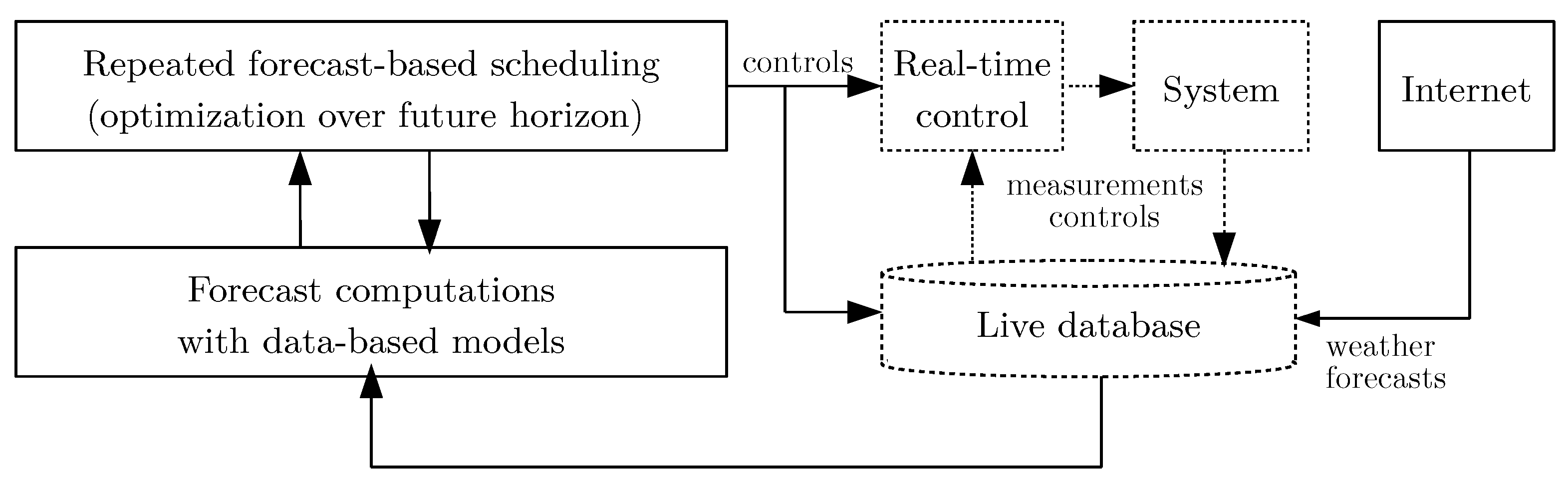
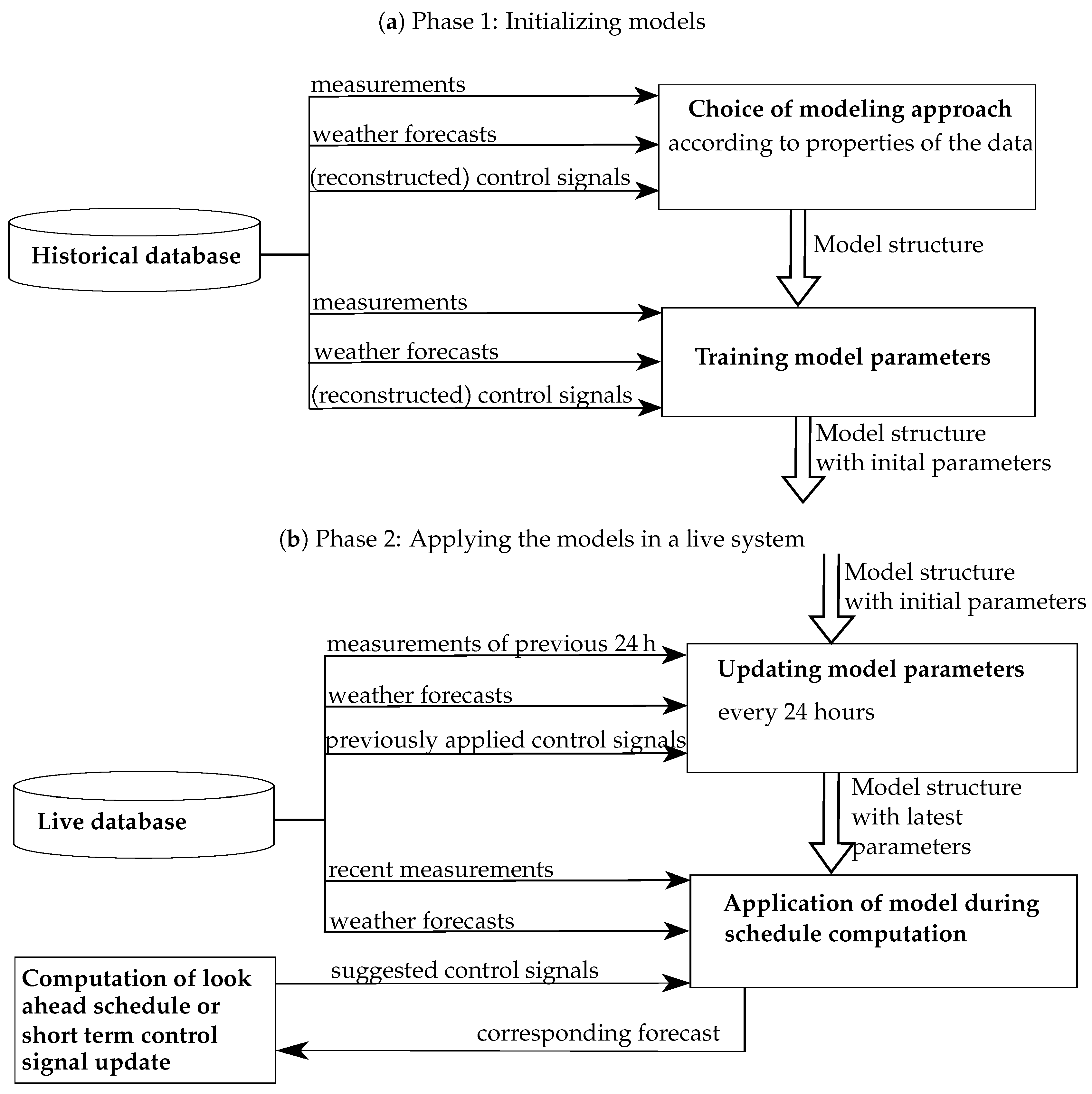
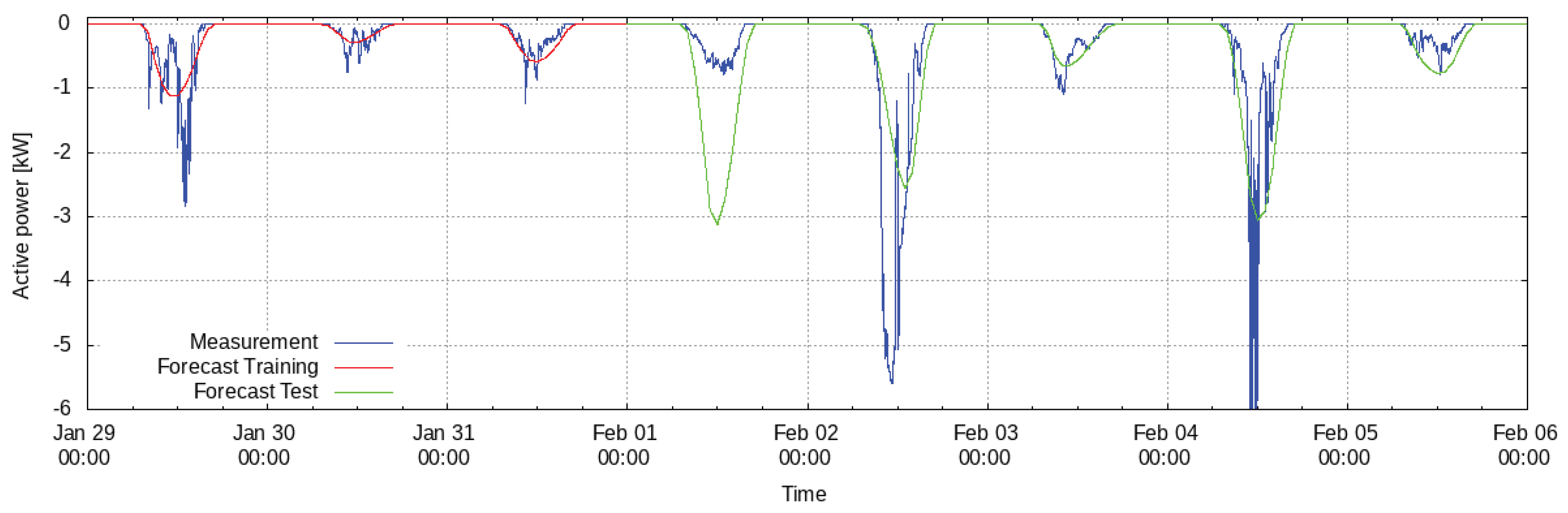
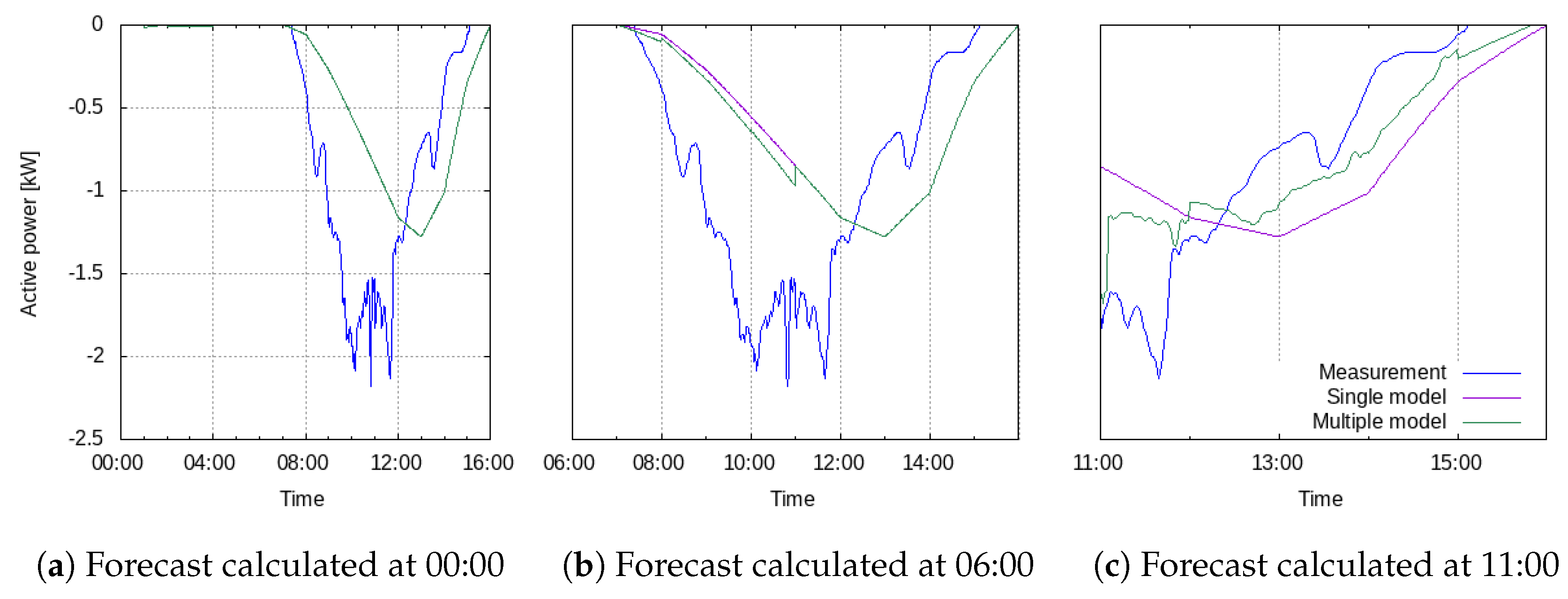
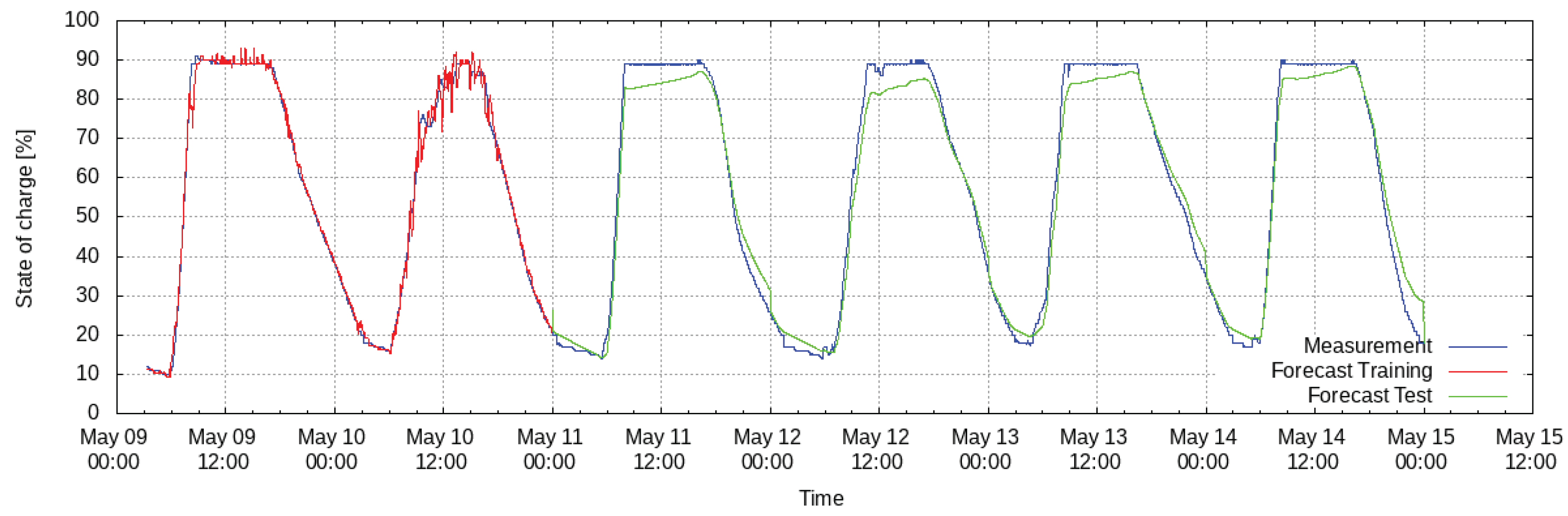
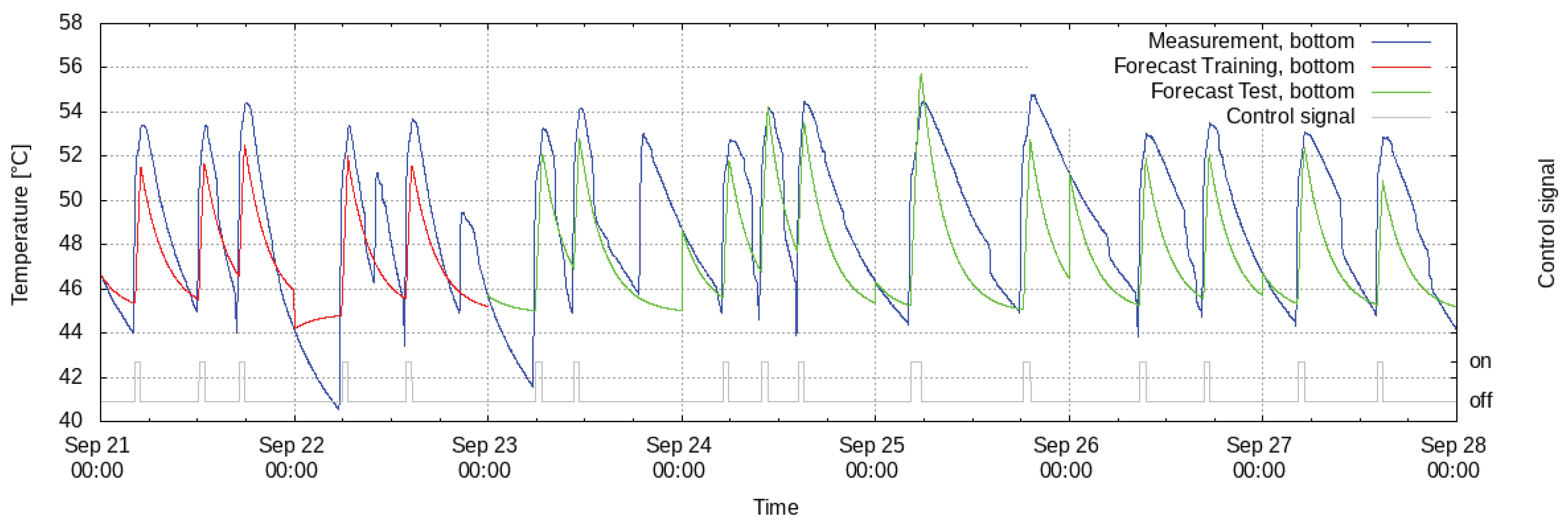
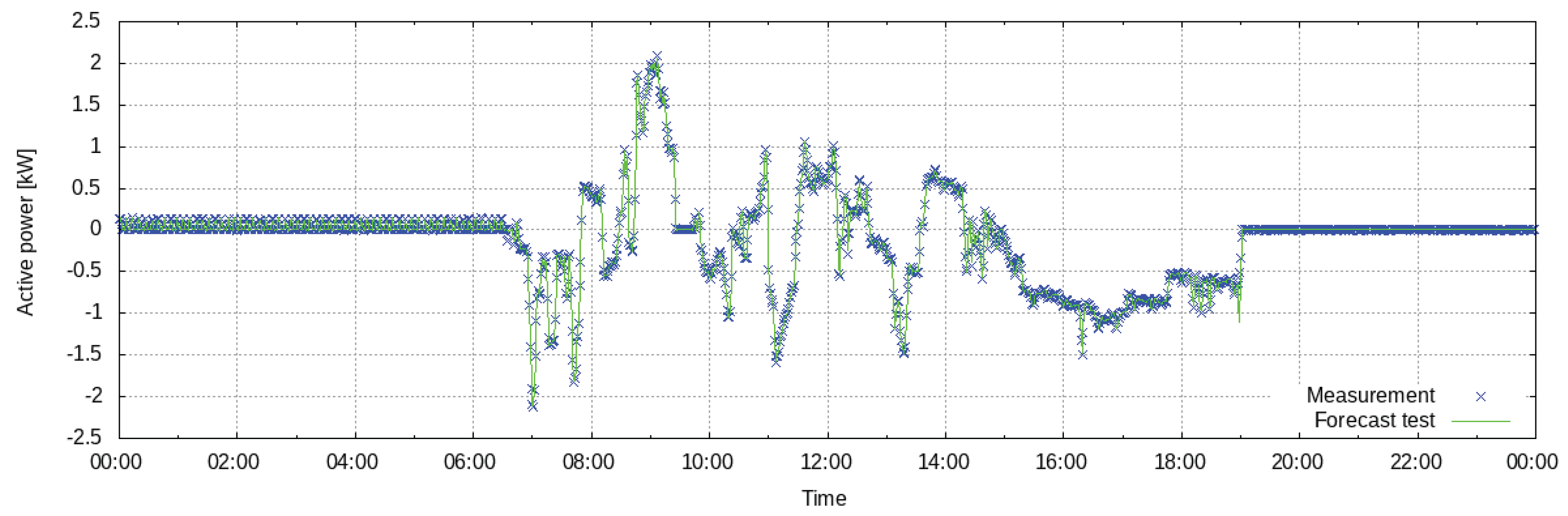
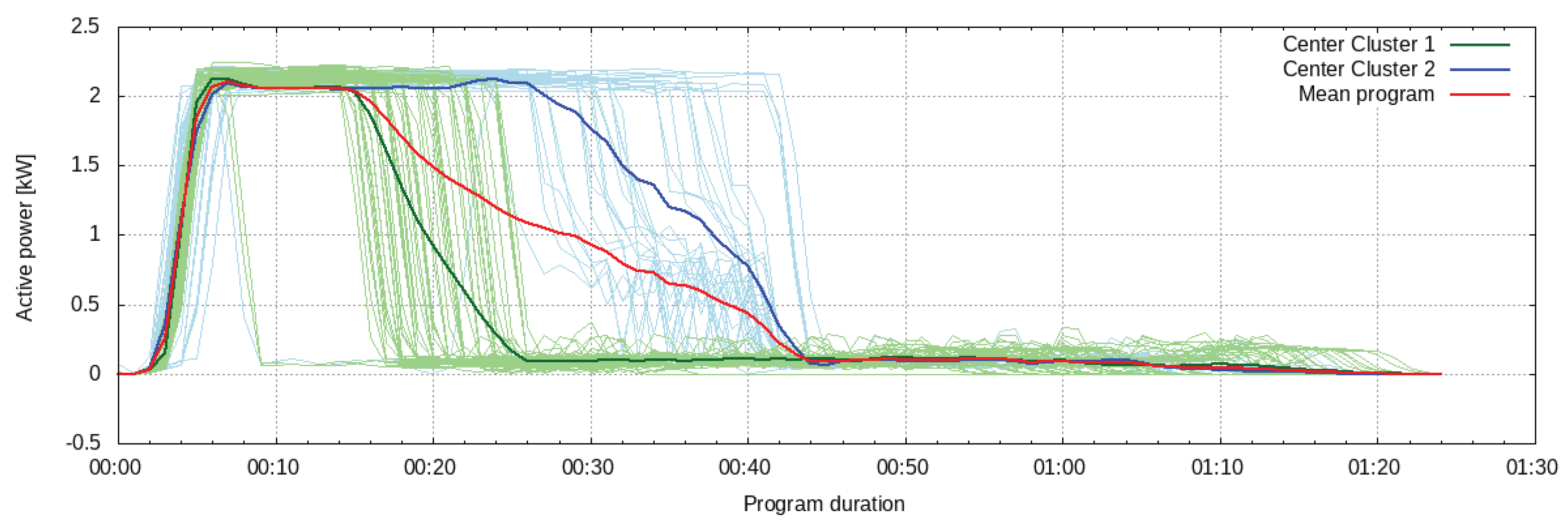
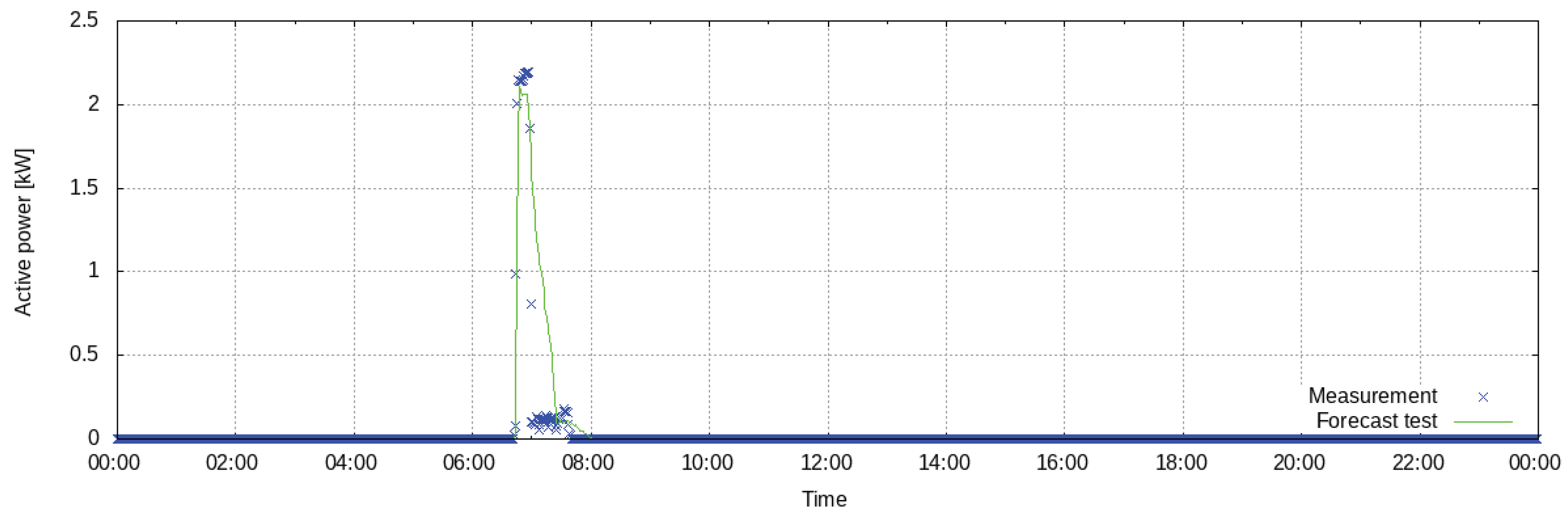
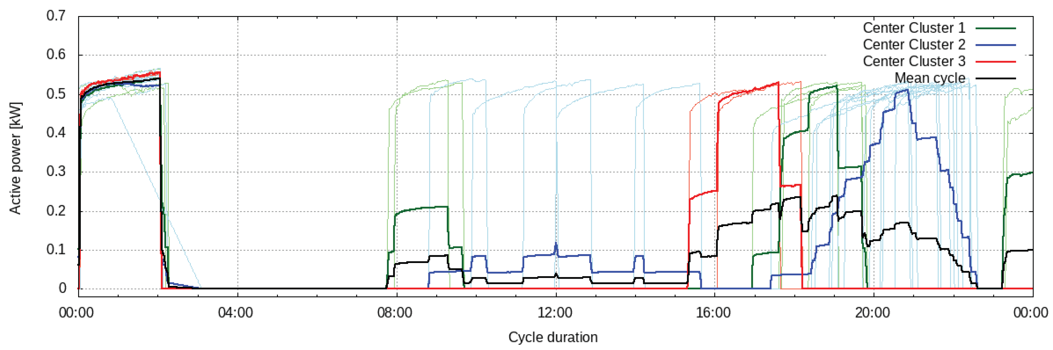
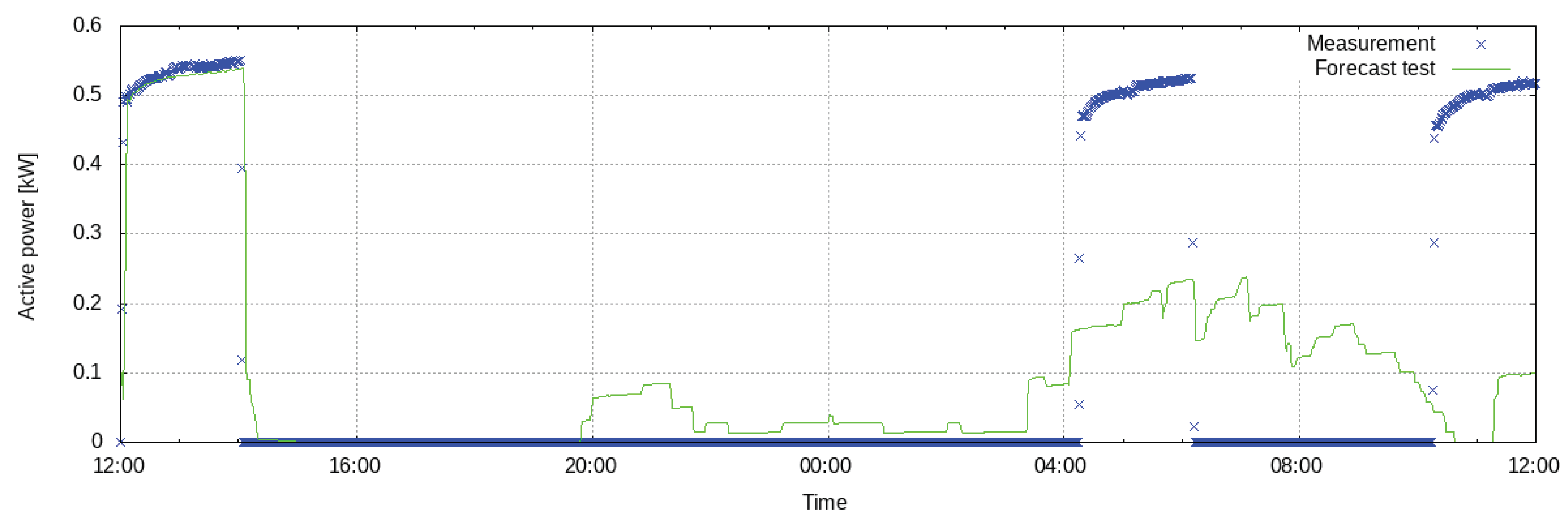
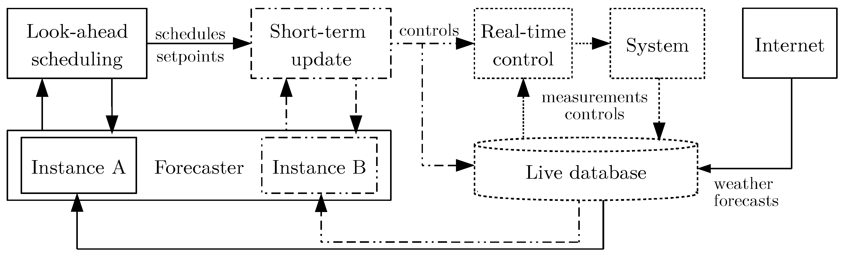
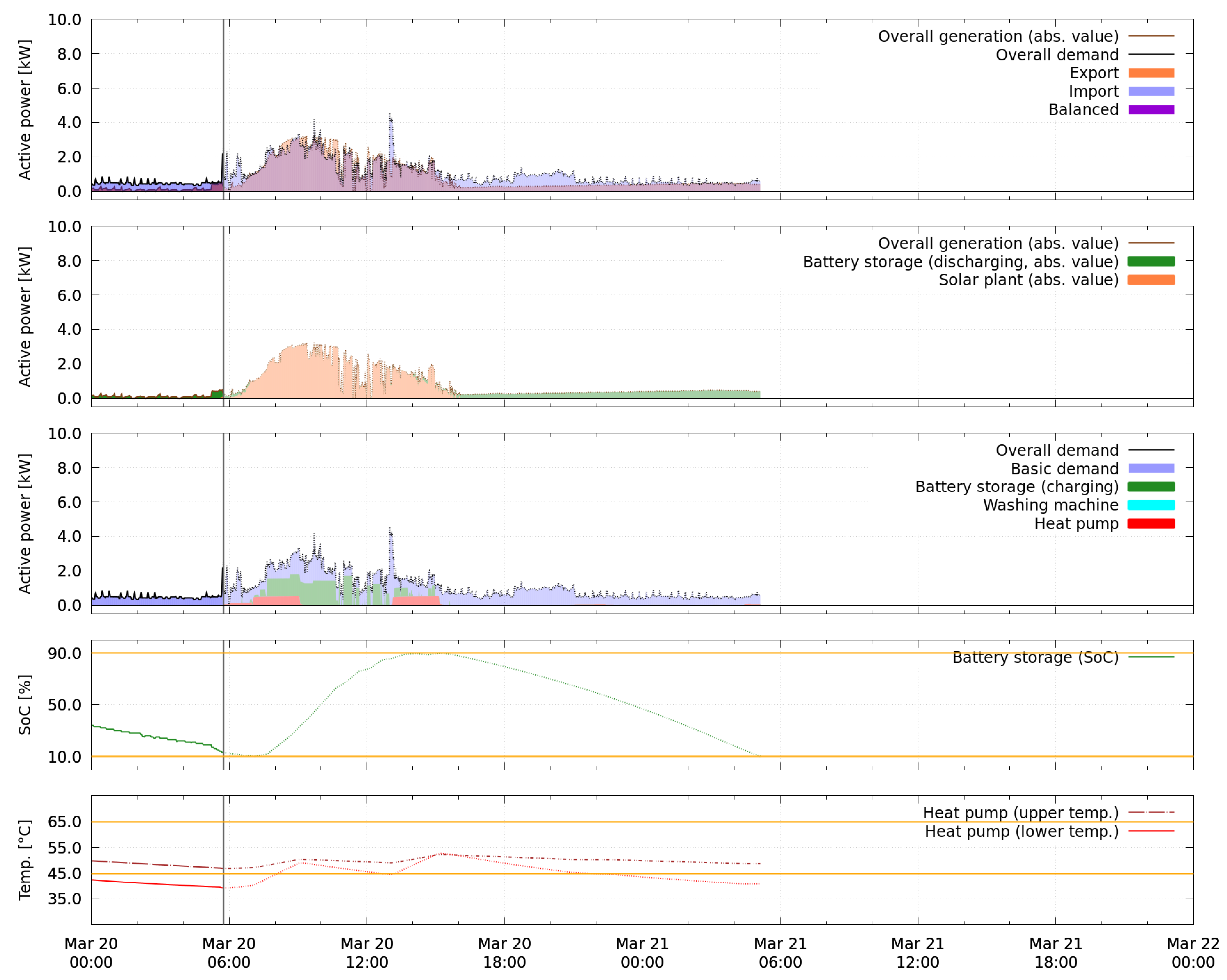
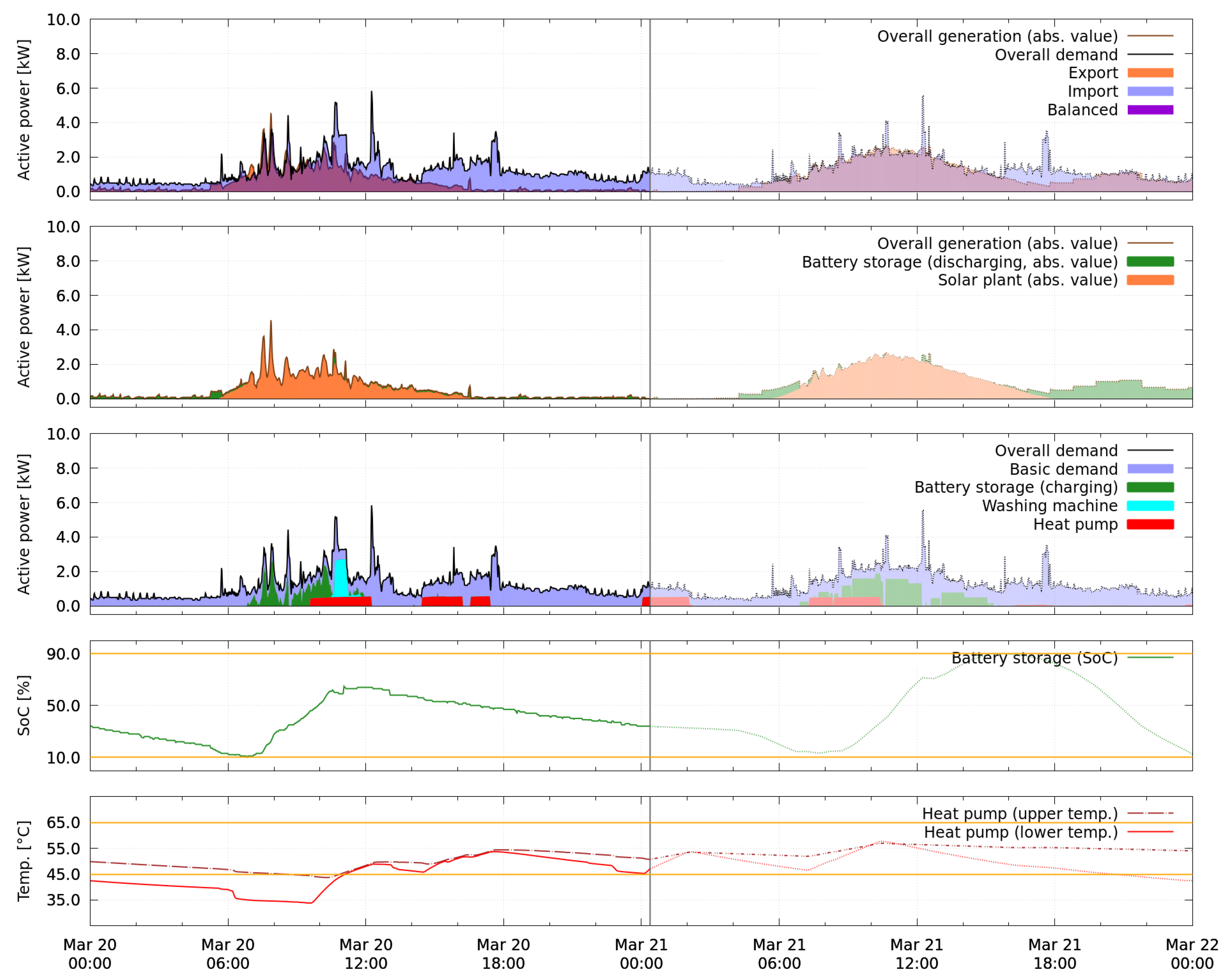
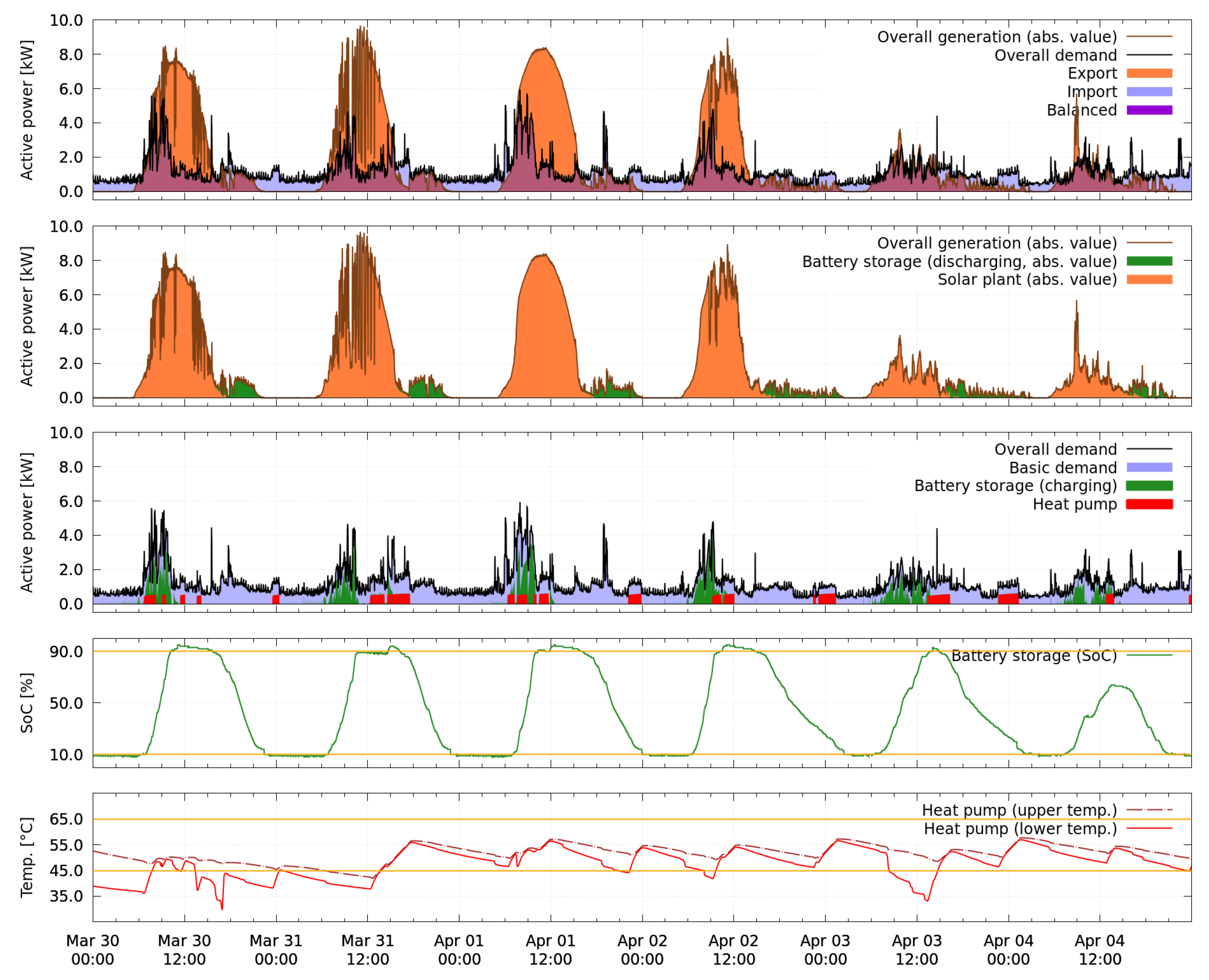
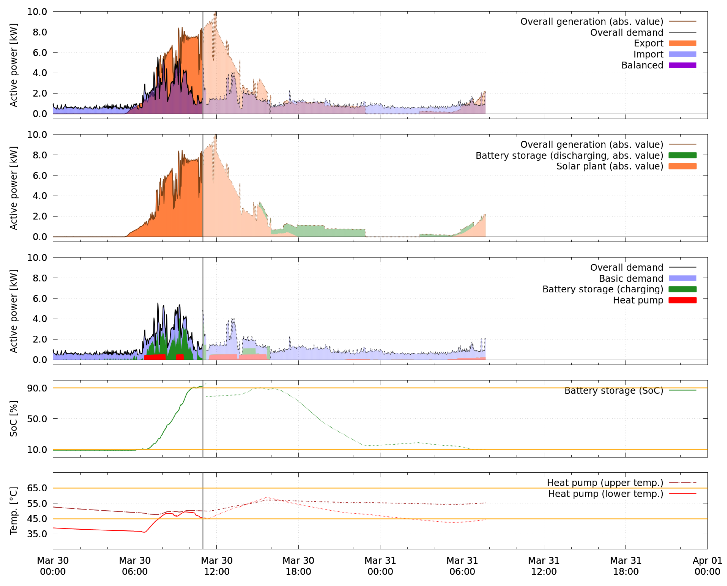
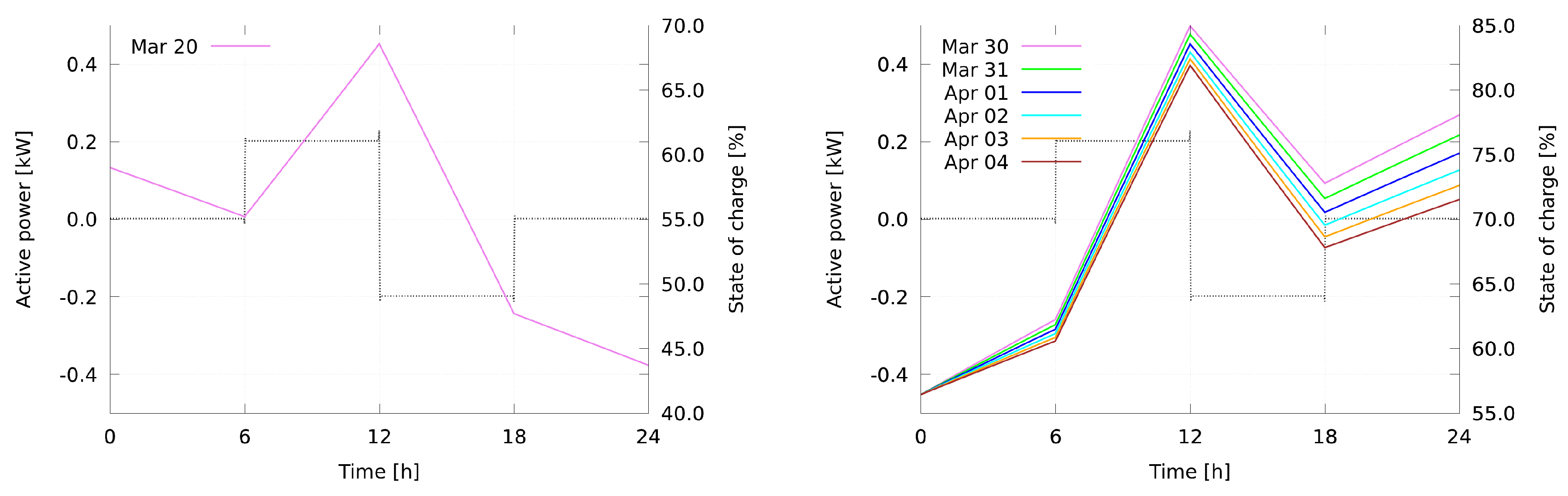
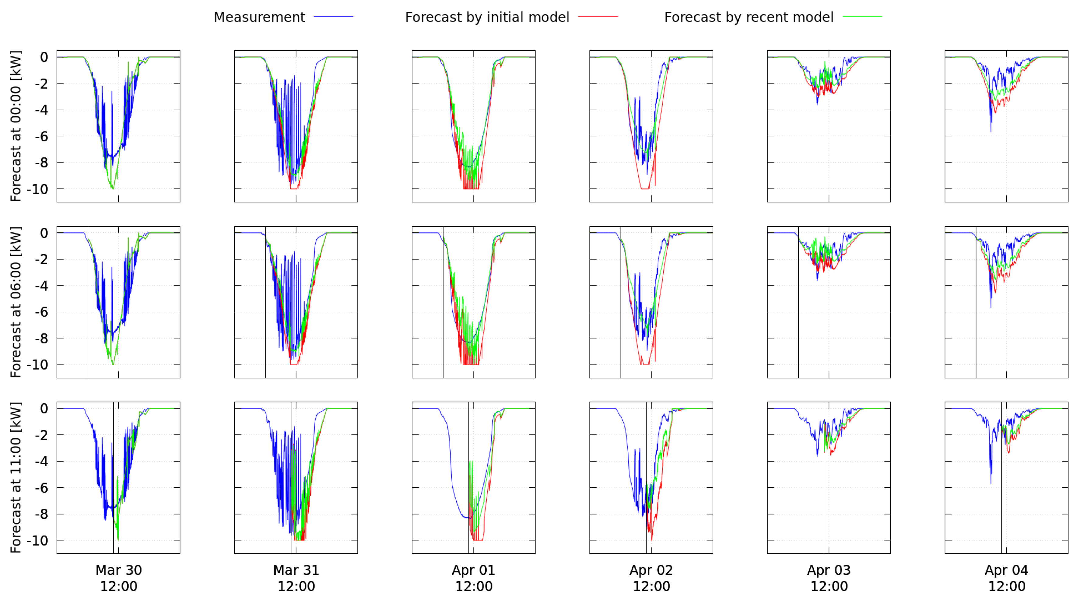
Table 1.
Overview of properties of the main devices on the the demonstration site. The term ‘uncontrolled’ as used in this table refers to a situation where a device is not controlled by the smart energy system, but it might still follow an internal control logic.
Table 1.
Overview of properties of the main devices on the the demonstration site. The term ‘uncontrolled’ as used in this table refers to a situation where a device is not controlled by the smart energy system, but it might still follow an internal control logic.
| Device | Properties | Control |
|---|---|---|
| Photovoltaic plant | Maximum power output of 9.8 kW via three-phase inverter. Surplus power which is not self-consumed directly is sold and exported to the distribution grid. | Uncontrolled operation in both Phases 1 and 2. |
| Washing machine | Regular device for households with up to 4 persons and 7–8 kg of clothes. | Uncontrolled in Phase 1, i.e., started by manual activation. In Phase 2, power supply can be interrupted and reestablished via a remotely controlled wireless socket. |
| Battery storage | Lithium-ion battery storage of 106 Ah capacity (5.5 kWh energy, usable 5.0 kWh) with one-phase inverter with maximum apparent power flow of 6 kVA. Discharge is stopped as soon as an exporting power flow is detected at the grid coupling point. | In both Phases 1 and 2, setpoints for active and reactive power are provided and communicated to the inverter via modbus protocol. |
| heat pump | Compact domestic hot water heat pump appliance with 0.5 kW nominal active power integrating 300 L water tank. Draws in warm ambient air directly at indoor installation site, exploiting waste heat from other appliances in the room (no outdoor component or permanent connection to outdoor air). | Uncontrolled in Phase 1, i.e., operating with internal hysteresis to track temperature setpoint. In Phase 2, temperature setpoint can be temporarily changed to higher value through usage of SG Ready interface, and a heat exchanger in the water tank connected to the household’s heating system can be activated additionally. |
Table 2.
Chosen devices with classification and method for model generation.
| Device | Class | Output | Model Behavior | Method | Model Assumptions |
|---|---|---|---|---|---|
| photovoltaic plant | generation | active power | continuous | regression | polynomial model of degree |
| washing machine | consumption | active power | finite-state | clustering | clusters of washing programs are of similar size and spatially grouped, the mean washing program is computed for forecasting based on the cluster centers |
| battery storage | storage | active power | continuous | regression | polynomial model of degree |
| state of charge | continuous | regression | polynomial model of degree | ||
| heat pump | storage | active power | finite-state | clustering | consumption patterns during the heating cycles are of similar size and spatially grouped, the mean heating cycle is computed for forecasting based on the cluster centers |
| temperatures | continuous | regression | polynomial model of degree |
Table 3.
Model inputs for all devices for the training (during Phase 1) and the forecasting (during Phase 2).
Table 3.
Model inputs for all devices for the training (during Phase 1) and the forecasting (during Phase 2).
| Device | Output | Model Inputs for Training | Model Inputs for Forecasting |
|---|---|---|---|
| photovoltaic plant | active power | solar radiation forecast, past measurements for solar radiation, brightness and active power | |
| washing machine | active power | past measurements of active power and reconstructed control signal (device activation) | control signal (device activation) |
| battery storage | active power | past measurements of specified state of charge and consumed active power | control signal specifying the state of charge |
| state of charge | state of charge measured 30 min ago, past measurements of active power | state of charge measured or forecasted 30 min ago, active power forecast | |
| heat pump | active power | past measurements of active power and reconstructed control signal (device activation) | control signal (device activation) |
| temperatures | temperatures measured 10 min ago, past measurements of active power, reconstructed SG Ready control signal | temperatures measured or forecasted 10 min ago, active power forecast, suggested SG Ready control signal | |
Table 4.
To take measured weather data into account when modeling the photovoltaic plant, the model based on weather forecast data is substituted by multiple models. Each of these models can calculate forecasts for different parts of a 24-h forecast horizon and uses different input data.
Table 4.
To take measured weather data into account when modeling the photovoltaic plant, the model based on weather forecast data is substituted by multiple models. Each of these models can calculate forecasts for different parts of a 24-h forecast horizon and uses different input data.
| Model No. | Forecast horizon | Input Data |
|---|---|---|
| 1 | [1 , 2 ] | Weather and power data measured 3 min ago |
| 2 | [3 , 5 ] | Weather and power data measured 6 min ago |
| 3 | [6 , 1 ] | Weather and power data measured 1 h 1 min ago |
| 4 | [1 1 , 3 ] | Weather and power data measured 3 h 1 min ago |
| 5 | [3 1 , 24 ] | Weather forecast and data measured 24 h 1 min ago |
Table 5.
Parameters and constraints used in the experimental setup.
| Parameter/Constraint | Value(s) | Unit |
|---|---|---|
| Control step size | 1 | min |
| Forecast horizon | 24 | h |
| Length of update interval for look-ahead scheduling | 30 | min |
| Max. length of look-ahead subintervals | 60 | min |
| Timeout of look-ahead scheduling optimization | 15 | s |
| Timeout of short-term update optimization | 15 | s |
| SAPHR time grid step width | 5 | min |
| SAPHR | 100.0 | - |
| SAPHR | 0.5 | - |
| SAPHR transitions per temperature level n | 40 | - |
| SAPHR decrease rate r | 0.9 | - |
| Discrete PHR box width [48] | 10 | - |
| Regular model update frequency | 1 | 1/day |
| Time for model update | 22:00 | UTC |
| Import price for energy from public grid | 0.24 | €/kWh |
| Export gain for energy from photovoltaic plant | 0.12 | €/kWh |
| Battery storage capacity | 5.5 | kWh |
| Lowest/highest allowed battery storage SoC | 10/90 | % |
| Min./max. battery power | −3.5/3.5 | kW |
| Min./max. heat pump temperature | 45/65 | °C |
| Max. number of heat pump activations | 4 | 1/day |
| Min./max. length of heat pump activation | 20/180 | min |
| Min. resting time between heat pump activations | 20 | min |
| Earliest/latest start of washing machine | 05:00/18:00 | UTC |
| Length of washing machine run | 240 | min |
Table 6.
Evaluation of first test period (20 March, 00:00 to 21 March, 00:00). All values except for the cost/profit are given as absolute values. The overall energy generated by the photovoltaic plant during the test period is 10.58 kWh.
Table 6.
Evaluation of first test period (20 March, 00:00 to 21 March, 00:00). All values except for the cost/profit are given as absolute values. The overall energy generated by the photovoltaic plant during the test period is 10.58 kWh.
| Import | Export | Cost (+) or | Battery Storage Energy (kWh) | |||||
|---|---|---|---|---|---|---|---|---|
| kWh | € | kWh | € | Profit (−) (€) | Charged | Discharged | Lost | |
| experiment | 16.58 | 3.98 | 0.73 | 0.09 | 3.89 | 3.27 | 2.11 | 1.17 |
| w/o battery storage | 17.69 | 4.25 | 3.00 | 0.36 | 3.89 | - | - | - |
| consumption only | 25.27 | 6.07 | - | - | 6.07 | - | - | - |
Table 7.
Evaluation of second test period (30 March at 00:00 to 5 April at 00:00). All values except for the cost/profit are given as absolute values. The overall energy generated by the photovoltaic plant during the test period is 216.67 kWh.
Table 7.
Evaluation of second test period (30 March at 00:00 to 5 April at 00:00). All values except for the cost/profit are given as absolute values. The overall energy generated by the photovoltaic plant during the test period is 216.67 kWh.
| Import | Export | Cost (+) or | Battery Storage Energy (kWh) | |||||
|---|---|---|---|---|---|---|---|---|
| kWh | € | kWh | € | Profit (−) (€) | Charged | Discharged | Lost | |
| experiment | 56.70 | 13.61 | 130.73 | 15.69 | −2.08 | 30.65 | 22.34 | 8.31 |
| w/o battery storage | 76.19 | 18.26 | 158.52 | 19.02 | −0.74 | - | - | - |
| consumption only | 133.93 | 32.14 | - | - | 32.14 | - | - | - |
Table 8.
Error values for Figure 19 all normalized to the largest value measured during those six days and calculated for the time interval from the forecast calculation until midnight.
Table 8.
Error values for Figure 19 all normalized to the largest value measured during those six days and calculated for the time interval from the forecast calculation until midnight.
| March 30 | March 31 | April 01 | April 02 | April 03 | April 04 | |||||||
|---|---|---|---|---|---|---|---|---|---|---|---|---|
| 1st | rec. | 1st | rec. | 1st | rec. | 1st | rec. | 1st | rec. | 1st | rec. | |
| 00:00 | 11.0% | 18.6% | 15.6% | 9.6% | 7.0% | 15.8% | 7.6% | 6.1% | 4.4% | 9.8% | 6.7% | |
| 06:00 | 12.7% | 21.6% | 18.1% | 11.6% | 9.2% | 18.1% | 9.2% | 6.8% | 5.8% | 10.8% | 7.6% | |
| 11:00 | 9.4% | 21.2% | 18.7% | 16.4% | 10.2% | 20.4% | 9.8% | 7.5% | 5.7% | 7.5% | 5.5% | |
Table 9.
Error values for evaluation of the most recent models of the respective day and the evaluation of their respective direct predecessors all normalized to the largest value measured during the six days of the second test period and calculated for the time interval from the forecast calculation until midnight.
| March 30 | March 31 | April 01 | April 02 | April 03 | April 04 | |||||||
|---|---|---|---|---|---|---|---|---|---|---|---|---|
| prev. | rec. | prev. | rec. | prev. | rec. | prev. | rec. | prev. | rec. | prev. | rec. | |
| 00:00 | 11.0% | 18.6% | 15.6% | 8.1% | 7.0% | 8.7% | 7.6% | 4.4% | 4.4% | 6.7% | 6.7% | |
| 06:00 | 12.7% | 21.6% | 18.1% | 10.0% | 9.2% | 10.0% | 9.2% | 5.9% | 5.8% | 7.6% | 7.6% | |
| 11:00 | 9.4% | 21.2% | 18.7% | 13.7% | 10.2% | 12.7% | 9.8% | 5.6% | 5.7% | 5.5% | 5.5% | |
© 2020 by the authors. Licensee MDPI, Basel, Switzerland. This article is an open access article distributed under the terms and conditions of the Creative Commons Attribution (CC BY) license (http://creativecommons.org/licenses/by/4.0/).
Share and Cite
MDPI and ACS Style
Lachmann, M.; Maldonado, J.; Bergmann, W.; Jung, F.; Weber, M.; Büskens, C. Self-Learning Data-Based Models as Basis of a Universally Applicable Energy Management System. Energies 2020, 13, 2084. https://doi.org/10.3390/en13082084
AMA Style
Lachmann M, Maldonado J, Bergmann W, Jung F, Weber M, Büskens C. Self-Learning Data-Based Models as Basis of a Universally Applicable Energy Management System. Energies. 2020; 13(8):2084. https://doi.org/10.3390/en13082084
Chicago/Turabian StyleLachmann, Malin, Jaime Maldonado, Wiebke Bergmann, Francesca Jung, Markus Weber, and Christof Büskens. 2020. "Self-Learning Data-Based Models as Basis of a Universally Applicable Energy Management System" Energies 13, no. 8: 2084. https://doi.org/10.3390/en13082084
Note that from the first issue of 2016, this journal uses article numbers instead of page numbers. See further details here.