Influence of Fluctuations in Fossil Fuel Commodities on Electricity Markets: Evidence from Spot and Futures Markets in Europe


1
Graduate School of Economics, Kobe University, Kobe 657-8501, Japan
2
The Kansai Electric Power Company, Incorporated, Osaka 530-8270, Japan
*
Author to whom correspondence should be addressed.
Energies 2020, 13(8), 1900; https://doi.org/10.3390/en13081900
Submission received: 4 March 2020
/
Revised: 8 April 2020
/
Accepted: 11 April 2020
/
Published: 13 April 2020
(This article belongs to the Special Issue Empirical Analysis of Natural Gas Markets)
Abstract
:Using a fresh empirical approach to time-frequency domain frameworks, this study analyzes the return and volatility spillovers from fossil fuel markets (coal, natural gas, and crude oil) to electricity spot and futures markets in Europe. In the time domain, by an approach developed by Diebold and Yilmaz (2012) which can analyze the directional spillover effect across different markets, we find natural gas has the highest return spillover effect on electricity markets followed by coal and oil. We also find that return spillovers increase with the length of the delivery period of electricity futures. In the frequency domain, using the methodology proposed by Barunik and Krehlik (2018) that can decompose the spillover effect into different frequency bands, we find most of the return spillovers from fossil fuels to electricity are produced in the short term while most of the volatility spillovers are generated in the long term. Additionally, dynamic return spillovers have patterns corresponding to the use of natural gas for electricity generation, while volatility spillovers are sensitive to extreme financial events.
1. Introduction
Electricity is traded in both spot and futures markets. Extensive research has been undertaken over the past two decades concerning the spot market for electricity (e.g., [1,2,3,4]). Electricity is a non-storable good and faces generation constraints, transmission constraints, and seasonal issues, which can cause a timing imbalance in trade and fluctuations in electricity prices in the spot market.
Electricity futures have often played two roles for investors. First, electricity futures are an essential indicator to predict future spot prices. Second, electricity futures provide investors who are willing to take positions in power markets an excellent risk management tool for reducing their risk exposure, by reducing the operational risks caused by high volatility in the electricity spot market. For this reason, electricity futures trading is more extensive than spot trading. There are also many studies concerning the electricity futures market (e.g., [5,6,7,8]).
Approximately half of the world’s electricity is generated by fossil fuels such as crude oil, natural gas, and coal. According to the BP Statistical Review of World Energy 2019 [9], in 2018, approximately 40.5% of electricity was produced by oil, gas, and coal sources in Europe, which also necessarily implies the possibility of the spillover effects across the fossil fuel markets and electricity market. Additionally, in Huisman and Kilic’s [5] study, they state that although electricity cannot be stored directly, it can be stored in the sense that fossil fuels are storable. The electricity producer who wants to sell an electricity futures contract can either purchase the amount of fossil fuels in the spot market and store it until the delivery period to fulfill the delivery agreement or purchase the fossil fuel futures instead of storing them directly. For this reason, the price of electricity futures may be related to the storage cost of fossil fuels. On the other hand, in electricity spot market, according to the Mosquera-López and Nursimulu’s [10] research, unlike futures markets, the electricity spot prices are more determined by renewable energy infeed and electricity demand but not the price of fossil fuels such as natural gas, coal, and carbon. Thus, our research aims to examine if there are some difference in the spillover effects of fossil fuel commodity markets on the electricity market and futures in Europe. Additionally, given that there are many types of electricity futures contracts in terms of their delivery periods, we further examine whether there are different spillover effects between fossil fuel commodities and electricity futures with monthly, quarterly, and yearly delivery periods. To the best of our knowledge, although there are several papers discussing the relationship between the fossil fuels and electricity futures market, the relationship between fossil fuels and the price of electricity futures with different delivery periods have not been studied in previous research yet. However, it will help electricity market investors to fully understand the information transmission between electricity markets and fossil fuel markets to make their portfolio optimization and hedge strategy better and more comprehensive.
Many studies have investigated the interdependent relationship between fossil fuel commodities and electricity markets. For example, Emery and Liu [11] studied the relationship between the prices of electricity futures and natural gas futures and found a cointegration between California–Oregon Border and Palo Verde electricity futures and natural gas futures. Mjelde and Bessler [12] used a vector error correction model to analyze the relationship between electricity spot prices and electricity-generating fuel sources (natural gas, crude oil, coal, and uranium) in the US. The authors found that the peak electricity price influences the natural gas price in contemporaneous time, while in the long term, apart from uranium, fuel source prices affect the electricity price. Based on the VECM model, Furió and Chuliá [13] analyzed the volatility and price linkages between the Spanish electricity market, Brent crude oil, and Zeebrugge (Belgium) natural gas. Natural gas and crude oil were seen to have an essential influence in the Spanish electricity market, with particular causality from the fossil fuel (Brent crude oil and Zeebrugge natural gas) markets to the Spanish electricity forward market.
Generalized autoregressive conditional heteroskedasticity (GARCH)-type models have also been used to study the relationship between electricity and fossil fuel markets. Serletis and Shahmoradi [14] used the GARCH-M model to investigate the linkages between natural gas and electricity prices and volatilities in Alberta, Canada, and found a bidirectional causality. Using the BEKK-GARCH model, Green et al. [15] measured the strength of volatility spillovers in the electricity market in Germany caused by volatility in natural gas, coal, and carbon emission markets. According to the results, during the sample period, natural gas and coal produced non-negligible spillovers while carbon emission markets caused spillover effects from 2011 to 2014.
The return spillover is defined as the cross-market correlation between price changes (returns) allowing for one market’s price fluctuation to affect the other market’s direction with a lag. On the other hand, the volatility spillover could capture the correlation between the size of price changes. That is, if one market becomes riskier over a period of time (which implies bigger price fluctuations) the riskiness of the interrelated market will also change. Measuring the return spillover could allow investors to evaluate the investment trends of markets while measuring the volatility spillover could enable investors to evaluate the risk information across markets. The information across markets provide useful insights into the portfolio diversification of investment, hedging strategies, and risk management for financial agents.
In this study, we analyze the return and volatility spillovers from the fossil fuel market commodities of natural gas, coal, and crude oil, to electricity spot and futures markets in Europe, by using two new empirical methods in the time-frequency domain: (1) the Diebold–Yilmaz approach; and (2) the Barunik and Krehlik methodology. The Diebold–Yilmaz approach was proposed in Diebold and Yilmaz [16] and developed in Diebold and Yilmaz [17]. In the Diebold–Yilmaz approach, the spillover index can be constructed based on the variance decomposition of forecast error, which allows for the study of the spillover effect with a fixed investment horizon in a quantitative way. However, investors have to consider different investment horizons when they make investment decisions because shocks may have different effects in the short and long term. For this reason, Barunik and Krehlik [18] used the Fourier transform to convert the Diebold–Yilmaz approach into the frequency domain so that the spillover index could be decomposed at different frequencies. Moreover, we can also obtain the time-varying spillover effect by using the moving window method. Many recent studies have used this method to study spillover effects and connectedness between assets, such as Singh et al. [19], Kang and Lee [20], and Malik and Umar [21]. In a more recent study, Lovcha and Perez-Laborda [22] used the Diebold–Yilmaz approach and the Barunik and Krehlik methodology to analyze the volatility connectedness between Henry Hub natural gas and West Texas Intermediate (WTI) crude oil in the time and frequency domains. Lau et al. [23] used the E-GARCH model and the Barunik and Krehlik methodology approach to investigate the return and volatility spillover effects among white precious metals, gold, oil, and global equity.
2. Method Framework
Diebold and Yilmaz [17] proposed an approach for measuring spillover in the generalized vector autoregression framework using the concept of connectedness, which built on the generalized forecast error variance decomposition (GFEVD) of a Vector Autoregressive (VAR) model with p lags.
where is an N × 1 vector of observed variables at time t, is the N × N coefficient matrices, and error vector with covariance matrix is possibly non-diagonal.
The VAR process can also be represented as the following Moving Average (∞) representation Equation (2), assuming the roots of lie outside the unit-circle:
where is an N × N coefficient matrix of infinite lag polynomials. Since the order of variables in the VAR system may have an influence on the impulse response or variance decomposition results, Diebold and Yilmaz [17] modified the generalized VAR framework of Koop et al. [24] and Pesaran and Shin [25] to ensure the variance decomposition’s independence of ordering. Under such a framework, the H-step-ahead generalized forecast error variance decomposition (GFEVD) can be presented in the form of Equation (3):
where stands for an N × N coefficient matrix of polynomials at lag h, and The represents H-steps ahead forecast error variance of the element j which is contributed by the k-th variable of the VAR system. To make the sum of the elements in each row of the generalized forecast error variance decomposition (GFEVD) equal to 1, each entry is standardized by the row sum as:
The is also defined as the Pairwise Spillover from k to j over the horizon H, which can measure the spillover effect from market k to market j. Meanwhile, there are also directional spillovers as defined by Diebold and Yilmaz:
Directional Spillovers (From): , the directional spillovers (From) measure the spillovers from all other markets to market k.
The above-defined measures of spillovers are summarized in Table 1.
Barunik and Krehlik [1] proposed a methodology that could decompose the spillover index in the Diebold–Yilmaz approach on the specific frequency bands.
First and foremost, by the application of the Fourier transform, spillovers in the frequency domain can be measured. Through a Fourier transform of the coefficients to obtain a frequency response function :=where i= The generalized causation spectrum over frequencies can be defined as:
It is crucial to note that represents the contribution of the k-th variable to the portion of the spectrum of the j-th variable at a given frequency . To find the generalized decomposition of variance to different frequencies, can be weighted by the frequency share of the variance of the j-th variable. The weighting function can be defined as:
Equation (6) gives a presentation of the power of the j-th variable at a given frequency, the sum of the frequencies to a constant value of 2π. Meanwhile, it is important to note that the generalized factor spectrum is the squared coefficient of weighted complex numbers and is a real number when the Fourier transform of the impulse is a complex number value. Therefore, we can set up the frequency band d = (a,b): a, b, a < b.
The GFEVD under the frequency band d is:
This also needs to be normalized; the scaled GFEVD on the frequency band d = (a,b): a, b, a < b can be defined as:
We can define as the pairwise spillover on a given frequency band d. Meanwhile, given the total spillover proposed by Diebold and Yilmaz [16], it is possible to define the total spillover on the frequency band d. Similarly, there are also directional spillovers in the frequency domain:
Frequency Directional Spillovers (From): , the frequency directional spillovers (From) represents the spillovers from all other markets to market k on the frequency band d.
3. Data and Preliminary Analysis
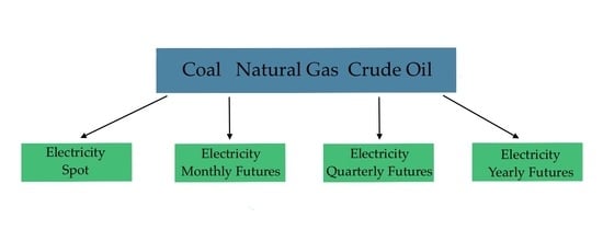
In this study, we use data from three fossil fuels markets: natural gas, coal, and crude oil; and four electricity markets: the electricity spot market and the monthly, quarterly, and yearly electricity futures markets. We employ daily data for the period from 2 January 2007, to 2 January 2019, with a total of 3019 observations. These data have been converted local currencies into euros at the daily exchange rate. All variables we used are listed in Table 3.
For the fossil fuels markets, we used a representative price of natural gas, coal, and crude oil futures markets in Europe. First, we used the United Kingdom (UK) National Balancing Point (NBP) natural gas futures to represent the natural gas market. The NBP natural gas market is the oldest natural gas market in Europe and is widely used as a leading benchmark for the wholesale gas market in Europe. Second, we used the Rotterdam coal futures to represent the coal market, which is financially settled based upon the price of coal delivered into the Amsterdam, Rotterdam, and Antwerp regions of the Netherlands. The futures contract is cash-settled against the API 2 Index, which is the benchmark price reference for coal imported to Northwest Europe. Third, we used the Brent crude oil futures to represent the crude oil market. The Brent crude oil market is one of the world’s most liquid crude oil markets. The price of Brent crude oil is the benchmark for African, European, and Middle Eastern crude. All futures mentioned above are traded on the Intercontinental Exchange (ICE) Futures Europe commodities market. The price of natural gas quoted in EUR per therm, the price of coal quoted in EUR per metric ton, and the price of crude oil quoted in EUR per barrel.
In Europe, electricity futures markets are offered in the European Energy Exchange (EEX). The EEX is a central European electric power exchange established in August 2000 and has become the leading energy exchange in Europe with more than 200 trading participants from 19 countries. In 2008, the power spot markets EEX and Powenext merged to create the European Power Exchange (EPEX SPOT) to offer spot markets in electricity. In this study, we used the spot, monthly futures, quarterly futures, and yearly futures markets of the Physical Electricity Index (Phelix) Baseload, which is the reference in Germany and majority of Europe. The electricity spot commodity is traded in the EPEX SPOT, and futures commodities are traded in the EEX. The prices of electricity spot and futures quoted in EUR per megawatt-hour (Mwh).
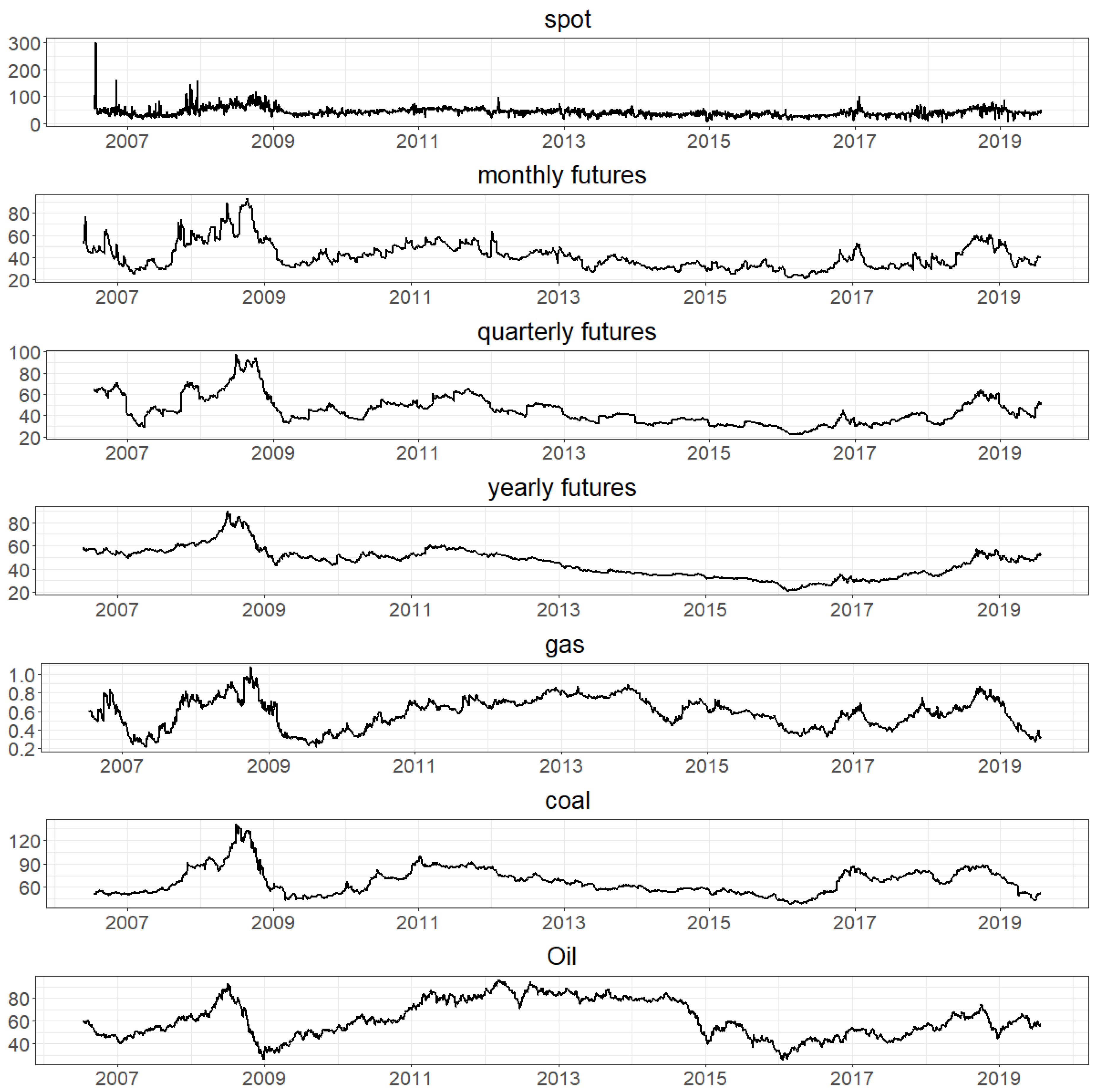
The closing prices of all variables are plotted in Figure 1. As shown, we find that the variation in electricity spot prices is more extreme, with more spikes and jumps than other commodities. It is clear that electricity futures and fossil fuel prices show a similar pattern.
In this study, we calculated the first order logged differences in prices as the returns and extracted the conditional variance series by fitting the AR-GARCH model as the volatilities. The descriptive statistics for the returns and volatilities of the variables are given in Table 4, where we can see, as expected, that the electricity spot market is the most volatile. The skewness value of the return of coal futures is negative and others are positive. Meanwhile, quarterly electricity futures have the highest skewness, indicating that they have the most extreme gains.
All of the returns and volatilities have a kurtosis value that is significantly higher than three, implying that the distribution of returns and volatilities will show tails that are peaked and fat. The highest kurtosis value is for quarterly electricity futures both in returns and volatilities.
The results of the Jarque–Bera (JB) test show that all returns and volatilities reject normality at the 1% significance level. Finally, since the Diebold–Yilmaz approach is based on the VAR model, the data should be stationary. From the results of the Augmented Dickey–Fuller (ADF) unit root test and the Philips and Pearron (PP) unit root test, the null hypothesis that of each variable being nonstationary is rejected at the 1% or 5% significance level for all cases.
4. Empirical Results and Discussion
First, we used a four-variable VAR model with four different sets of variables (four sets of returns and four sets of volatilities): The first set is , the second set is , the third set is , and the fourth set is . For the four sets of returns, according to the Schwarz Criterion (SC), the lag length of the VAR model is 4 in the first set and 1 in the other sets, while in the four sets of volatilities, the lag length of the VAR model is 2 in the first set and 1 in the other sets. Subsequently, the Diebold–Yilmaz approach, which is based on the generalized variance decomposition, is applied to the VAR models to assess the direction and intensity of the spillover index across the selected variables in the time domain.
Second, with the assistance of the Barunik and Krehik [18] methodology and following the methods of Toyoshima and Hamori [27], the spillover indexes obtained by the Diebold–Yilmaz approach were decomposed into three frequency bands: the high frequency, ‘Frequency H’, roughly corresponding to 1–5 days; the medium frequency, ‘Frequency M’, roughly corresponding to 5–21 days; and the low frequency, ‘Frequency L’, roughly corresponding to 21 days to infinity.
Finally, as noted by Barunik and Krehik [18], the methodology does not work if the forecasting horizon (H) < 100; therefore, the 100-days ahead forecasting horizon (H) for generalized variance decomposition was used in this study.
With the assistance of the Diebold–Yilmaz approach, Table 5 shows the return spillover effects from the three fossil fuels to the electricity spot market and the three types of futures markets. In addition, the last column of the table labelled ‘Directional Spillover (From)’ shows the total spillover effect from all fossil fuel commodities combined on the electricity spot market.
Table 5 highlights several important findings. First, as shown in each row of the table, for both spot and futures markets, natural gas is the largest contributor to the forecast error variance decomposition (FEVD) of electricity return, which further implies that natural gas has the most influence on the electricity return. Meanwhile, among the three fossil fuels, crude oil has the least influence upon the electricity return. This may be due to electricity production from one specific fuel and storage costs. According to the BP Statistical Review of World Energy 2019 [9], in Europe, from 2007 to 2018, almost 25.35% of electricity was produced from coal, followed by 18.88% from natural gas, and 2.02% from crude oil. This explains why crude oil has the least influence upon the electricity return. Fama and French [28] state that a trader can offset the risk of positions they have in a forward contract by holding a long or short inventory in the underlying commodity. Huisman and Kilic [5] note that although electricity cannot (yet) be stored directly, it can be stored in the sense that fossil fuels are storable. When an electricity producer sells an electricity futures contract, they have two choices: (1) purchase the amount of fossil fuels in the spot market and store it until the delivery period to fulfill the delivery agreement or; (2) purchase the fossil fuel futures instead of storing them directly. If the fuels have a high storage cost, the electricity producers would prefer to hold a futures contract on the fuels rather than purchase them in the spot market and store them directly. Compared to coal and crude oil, natural gas has higher storage costs and, therefore, the electricity producer would prefer to purchase natural gas futures. This further explains the high connectedness of electricity and natural gas futures markets. Based on high demand and high storage costs, it is not difficult to understand why natural gas futures have the most influence on the returns of electricity.
Second, it is interesting to note that the most significant return spillover effects are seen in yearly electricity futures, followed by the spillover effect to quarterly futures, then monthly futures. The return spillovers from fossil fuel commodities is the least in the electricity spot market. Under the assumption of storage costs mentioned earlier, when an electricity producer sells an electricity futures contract with a long delivery period, they would prefer to purchase futures contracts on underlying fuel commodities, rather than purchase them in the spot market and store until the delivery period. This implies that the return spillovers from fuel futures to electricity futures with a long delivery period are higher than to electricity futures with a short delivery period. Mosquera-López and Nursimulu [10] explored the drivers of German electricity prices in spot and futures markets and found that spot prices are determined by renewable energy infeed and electricity demand, while in futures markets prices are determined by the price of fossil fuels such as natural gas, coal, and carbon. This may explain why the return spillovers from fossil fuel commodities to electricity futures are higher than to electricity spot prices.
The return spillover results of Barunik and Krehil [16], which decompose the Diebold–Yilmaz spillover indexes into three different frequencies, are presented in Table 6. The spillovers from fossil fuel commodities to electricity markets are highest in the high frequency, followed by the medium frequency and the low frequency. This indicates that return shocks are transmitted from fossil fuel markets to electricity markets within only one week.
Table 7 shows the volatility spillover effects from the threVe fossil fuel commodities to the electricity spot market and the three types of futures. The results are unusual; among the three fossil fuel markets, natural gas has the highest volatility spillovers to electricity spot markets (0.691%), monthly (9.539%), and quarterly futures (3.565%), but not to yearly futures (0.145%). Additionally, oil exhibits the weakest volatility spillovers to all electricity markets (0.098%, 0.417%, and 0.211%, respectively), again, with the exception of yearly futures (1.835%).
In addition, in contrast to the return spillover results, the volatility spillovers from natural gas to monthly electricity futures (9.539%) is higher than for electricity futures with a longer delivery period. However, crude oil and coal transmit the highest volatility spillovers to yearly futures, while the spillovers to monthly futures are higher than to quarterly futures. Finally, with the exception of natural gas, both volatility spillovers and return spillovers are higher for electricity futures than for the electricity spot market.
Table 8 displays the volatility spillover results in the frequency domain. In contrast to the results in Table 6, the total volatility spillover is higher in the low frequency than in the high frequency. This indicates that the transmission of volatility shocks from fossil fuel markets to electricity markets is slower than that of return spillovers. The transmitted shocks from fossil fuels have long-lasting effects on electricity market volatility.
It is well established that financial markets can be affected by extreme events such as financial crises, price fluctuations, and market turmoil. For this reason, this section of our paper aims to capture the dynamics of spillover, in particular to investigate how spillovers from the fossil fuel market to the electricity market may change under extreme events. To accomplish this, a moving windows analysis with a 400-day window length was applied.
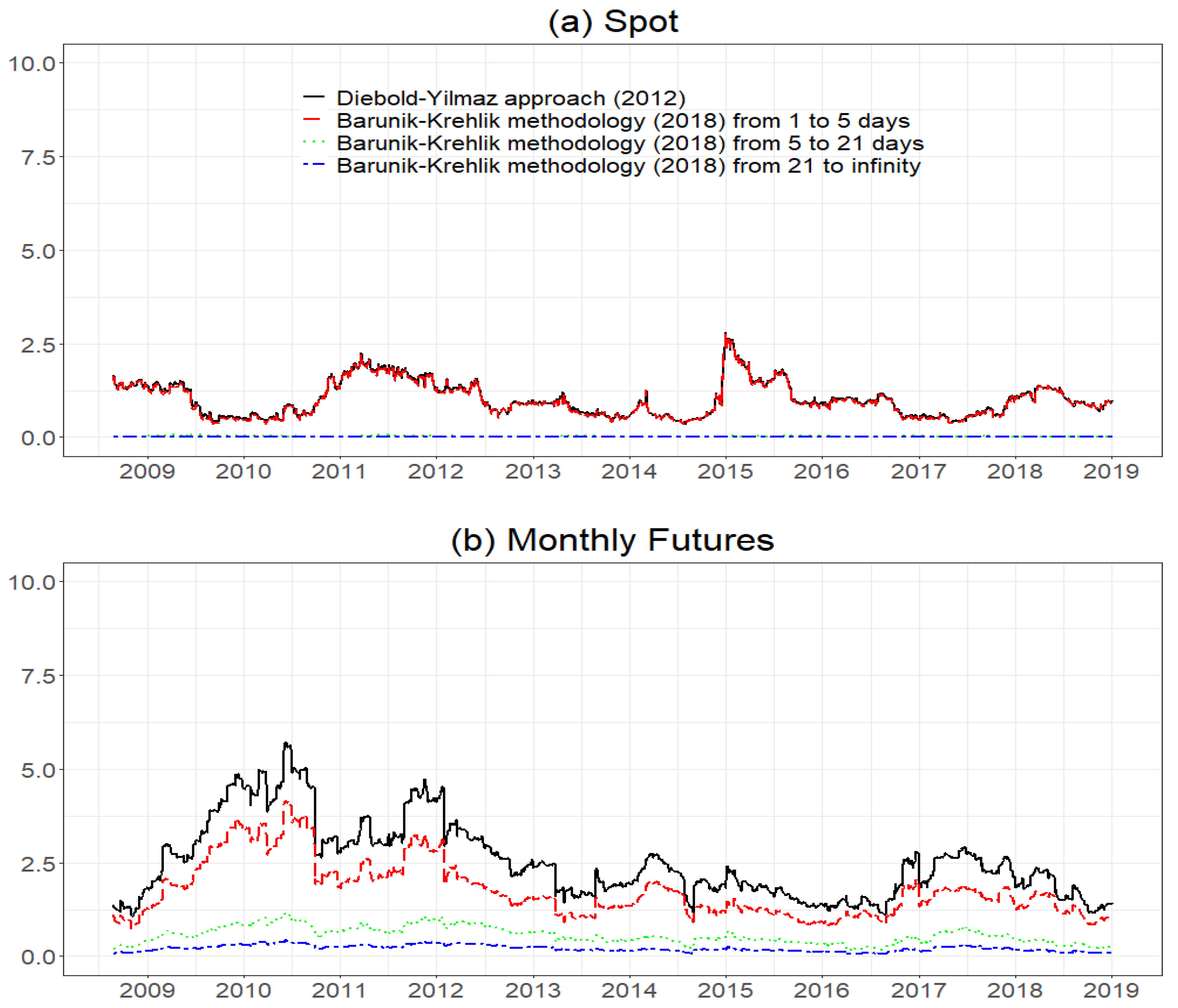
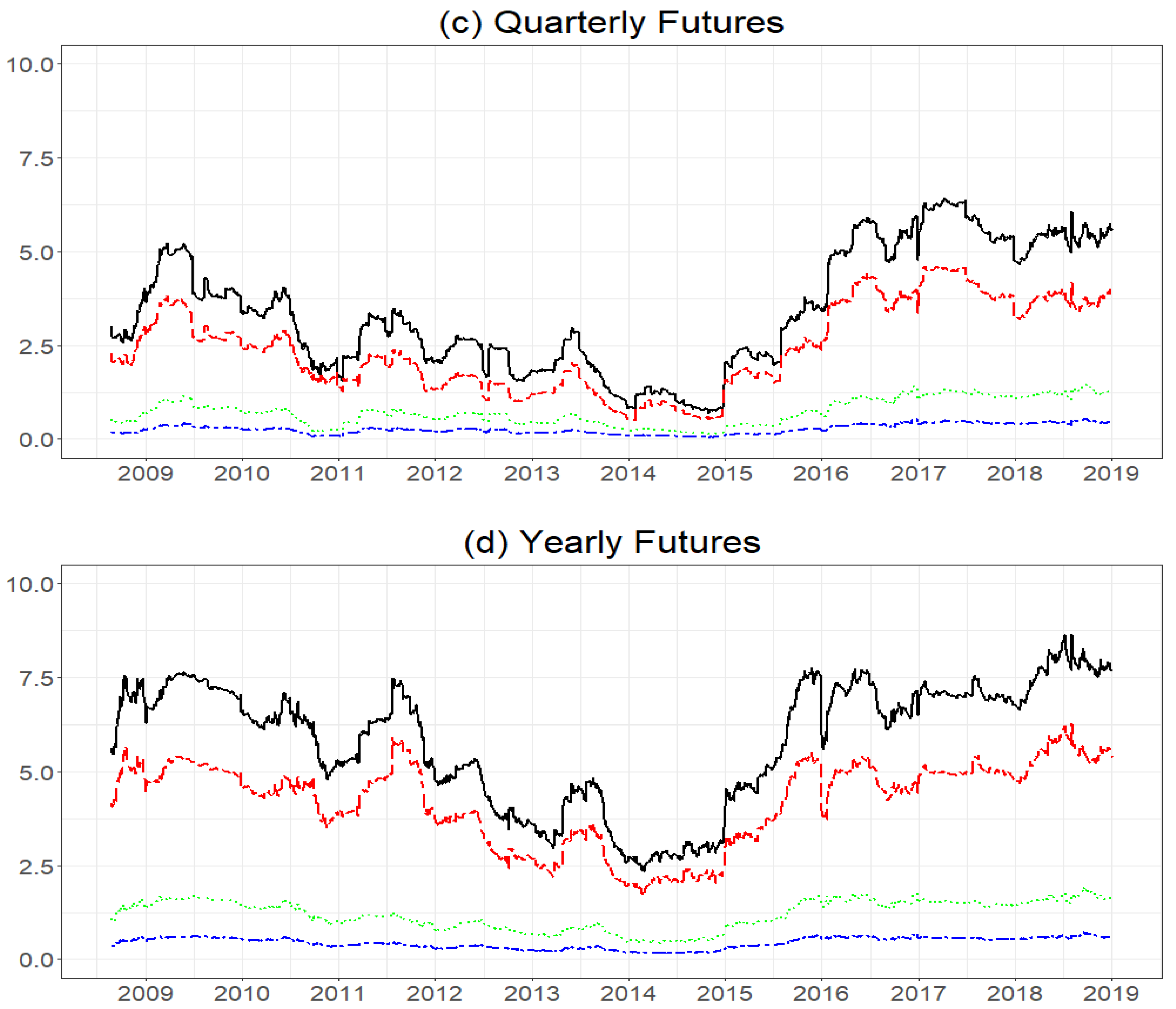
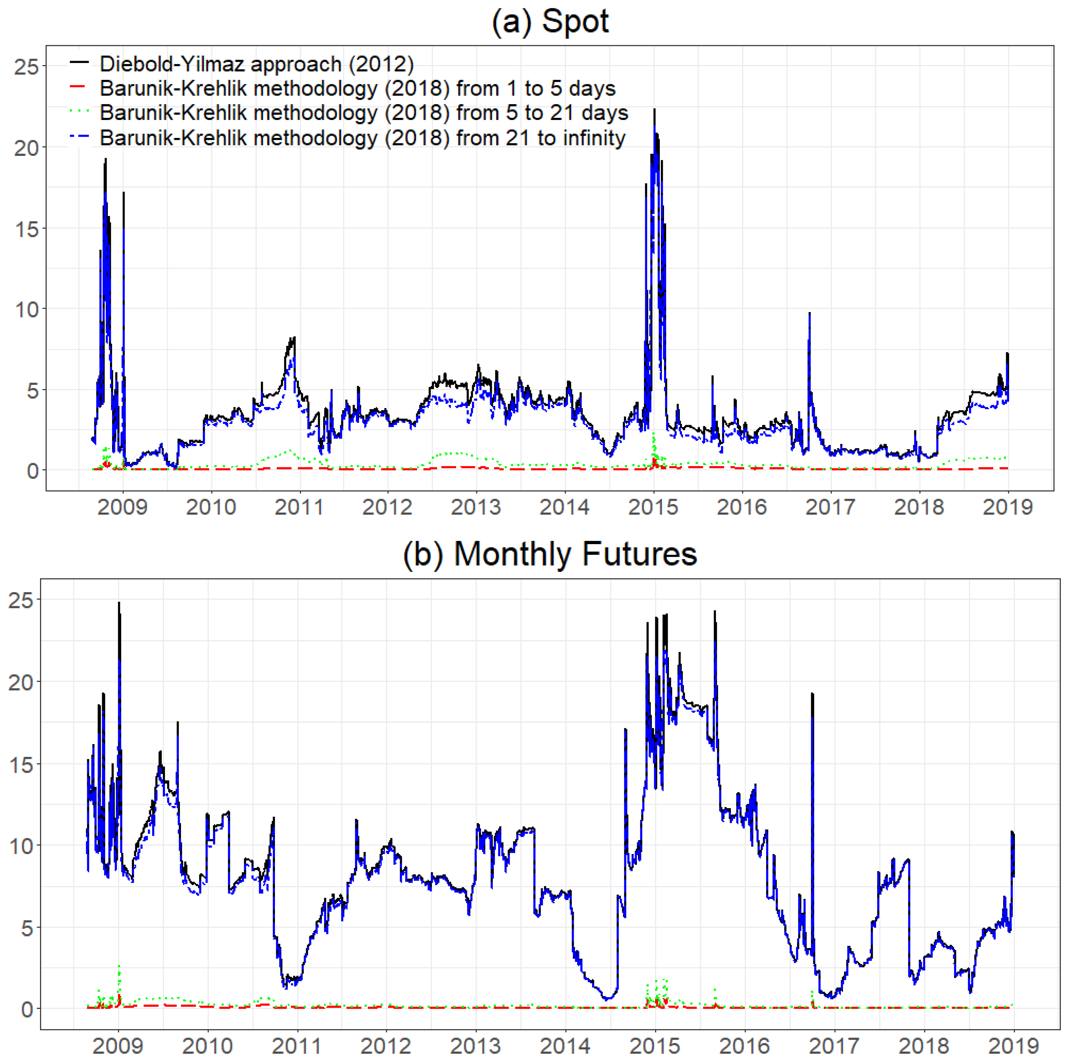
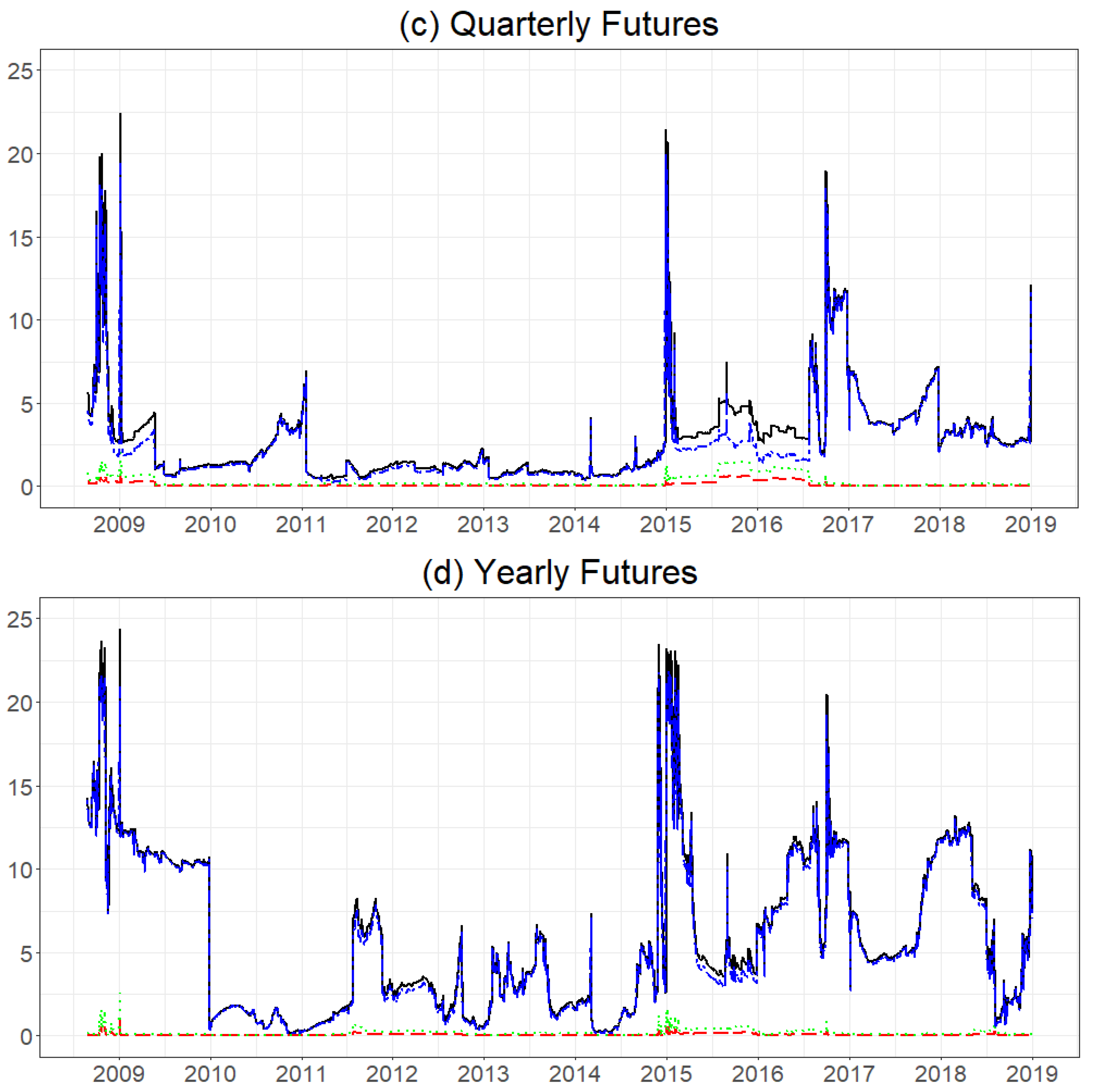
Figure 2 presents the dynamic directional return spillover from all fossil fuel commodities to electricity markets, measured by the Diebold–Yilmaz approach (2012) and the Barunik–Krehlik methodology (2018). The pairwise directional return spillovers are shown in Figure A1 in the Appendix A. In Figure 2, the solid line refers to the time-varying spillover of the Diebold–Yilmaz approach (2012), the long-dash line refers to spillover in the high frequency (1–5 days), the dotted line refers to spillover in the medium frequency (5–21 days), and the two-dash line refers to spillover in the low frequency (over 22 days). The results in Figure 2 indicate various characteristics.
First, the spillover effect of all three fossil fuel commodities to yearly electricity futures vary from 0% to 8.7%, followed by quarterly futures (0% to 6.3%), monthly futures (0% to 5.8%), and the spot market (0% to 2.8%). According to the results, it can be concluded that the return spillovers from fossil fuel commodities to electricity futures with a long delivery period are higher than to those with a short delivery period and that the return spillover effect is lowest in the electricity spot market. This is consistent with the results of the statistical analysis in Table 5.
Second, the spillovers from all three fossil fuel commodities to electricity markets are highest in the high frequency category, followed by the medium frequency and low frequency categories. This is also consistent with the results of the statistical analysis, shown in Table 6.
On the other hand, the proportion of spillovers from fossil fuel commodities to electricity futures in the medium frequency and low frequency categories are higher than to the electricity spot market in those frequencies. Compared to electricity spot, it appears that the spillovers to electricity futures are higher in the long term. There is an implicit possibility that the speed of information transmission from fossil fuel commodities to electricity futures is slower than to electricity spot.
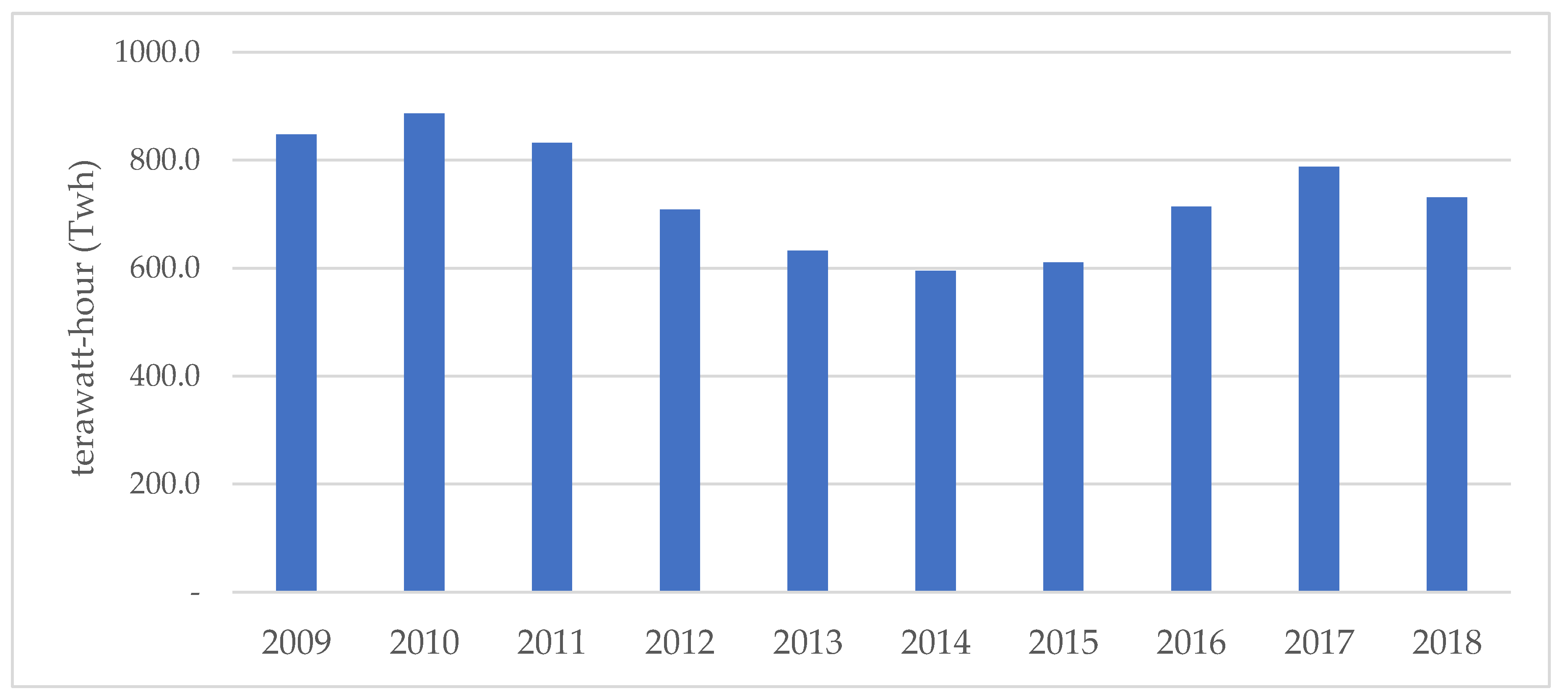
Finally, it is clear that the patterns of return spillovers from fossil fuel commodities to electricity spot and futures markets are quite different. As we mentioned before, spot prices are determined by renewable infeed and electricity demand while futures prices are determined by fossil fuels and mostly influenced by natural gas. We find that the directional spillover from fossil fuel commodities to the electricity futures market, especially quarterly futures and yearly futures, has some similar patterns with the change of electricity production toward natural gas in Europe. For example, the spillovers to quarterly and yearly futures decreased until 2015 but then tended to increase thereafter. This closely corresponds with the changes in electricity production using natural gas in Europe, which decreased from 2010 to 2015 and has since increased, as indicated by Figure 3.
The findings regarding dynamic directional volatility spillover from all fossil fuel commodities to electricity markets are presented in Figure 4 (The pairwise directional volatility spillovers are shown in Figure A2 in the Appendix A). First, it appears that the volatility spillover evolves more fiercely in contrast to return spillovers. In particular, there are many sharp increases, or fluctuations, corresponding to extreme events. This further indicates that volatility spillovers may be more sensitive to extreme events than return spillovers. For example, there are three significant sharp fluctuations in 2009, 2015, and 2016, possibly influenced by the 2008 global financial crisis, the 2014 international oil price’s violent shock, and the 2016 rise of coal and natural gas prices. Additionally, the proportions of volatility spillovers from fossil fuel commodities to electricity markets in the high frequency and low frequency categories also increased when the extreme events occurred.
Second, the volatility spillovers from all three fossil fuel commodities to electricity markets are highest in the low frequency category, followed by medium frequency and then high frequency, which is consistent with the results of the statistical analysis in Table 8.
5. Conclusions
This study analyzed return and volatility spillover effects from coal, natural gas, and crude oil fossil fuel markets to electricity spot and futures markets in Europe from 2 January 2007, to 2 January 2019, using a new empirical method in the time-frequency domain frameworks developed by Diebold and Yilmaz [17] and Barunik and Krehlik [18]. The study obtained the following major findings.
First, natural gas has the highest return spillover effect upon the electricity spot market and futures markets, followed by coal and crude oil. The results may be explained by two factors: (1) electricity production favoring one specific fossil fuel and; (2) the different storage cost of fossil fuels.
Second, due to increasing storage costs over time, the return spillovers from fossil fuel commodities to electricity futures with a long delivery period are higher than to electricity futures with a short delivery period. Meanwhile, compared to electricity futures markets, the spot market is more dependent on renewable energy infeed and electricity demand than fossil fuels such as natural gas and coal. Thus, the return spillover effect on electricity futures is higher than on electricity spot markets.
Third, in the frequency domain, we found that the majority of return spillover is generated in the short term which further implies that return shocks are transmitted from fossil fuel markets to electricity markets within only one week.
Contrary to expectations, we found that among the three fossil fuel markets, natural gas has the highest volatility spillover effect on electricity spot markets and monthly and quarterly futures, but not on yearly futures. Similarly, oil exhibits the weakest volatility spillover effect on all electricity markets, also except yearly futures markets.
Additionally, the volatility spillover from natural gas to monthly electricity futures is higher than for electricity futures with a longer delivery period. Meanwhile, crude oil and coal cause the highest volatility spillovers to yearly electricity futures, followed by monthly and then quarterly futures. Except for natural gas, the volatility spillovers from coal and crude oil to electricity futures are higher than in the electricity spot market, which is the same result as that found in the analysis of return spillovers.
In the frequency domain, the majority of volatility spillover is produced in the long term which further indicates that transmitted shocks from fluctuations in fossil fuels have long-lasting effects on electricity market volatility.
Furthermore, we also explored dynamic spillovers by adopting the 400-day moving window method. We found there is a similar pattern in the dynamics of return spillovers from fossil fuel commodities to electricity futures with long delivery periods, and to electricity generation from natural gas. However, we found the dynamic volatility spillovers from fossil fuels to electricity markets are more sensitive to extreme events such as the 2008 global financial crisis, the 2014 international oil price’s violent shock, and the 2016 rise in coal and natural gas prices, as shown by volatility spillovers varying sharply when the extreme events occurred.
The results in this paper may be helpful for investors with different investment horizons in Europe to diversify their portfolios, hedge their strategies, and make their risk management plans. For short term investors, constructing well-diversified portfolios consisting of fossil fuels futures, electricity spot and futures is a complicated task, especially in times of financial turmoil. On the other hand, for long-term investors, including the fossil fuels in portfolios composed primarily of electricity spot and futures with different delivery periods could enable them to obtain the long-term diversification benefits.
Author Contributions
Conceptualization, T.N. and S.H.; investigation, T.L. and X.H.; writing—original draft preparation, T.L.; writing—review and editing, X.H., T.N., and S.H.; project administration, S.H.; funding acquisition, S.H. All authors have read and agreed to the published version of the manuscript.
Funding
This work was supported by JSPS KAKENHI Grant Number 17H00983.
Acknowledgments
We are grateful to Keukwan Ryu and two anonymous referees for helpful comments and suggestions.
Conflicts of Interest
The authors declare no conflict of interest.
Appendix A
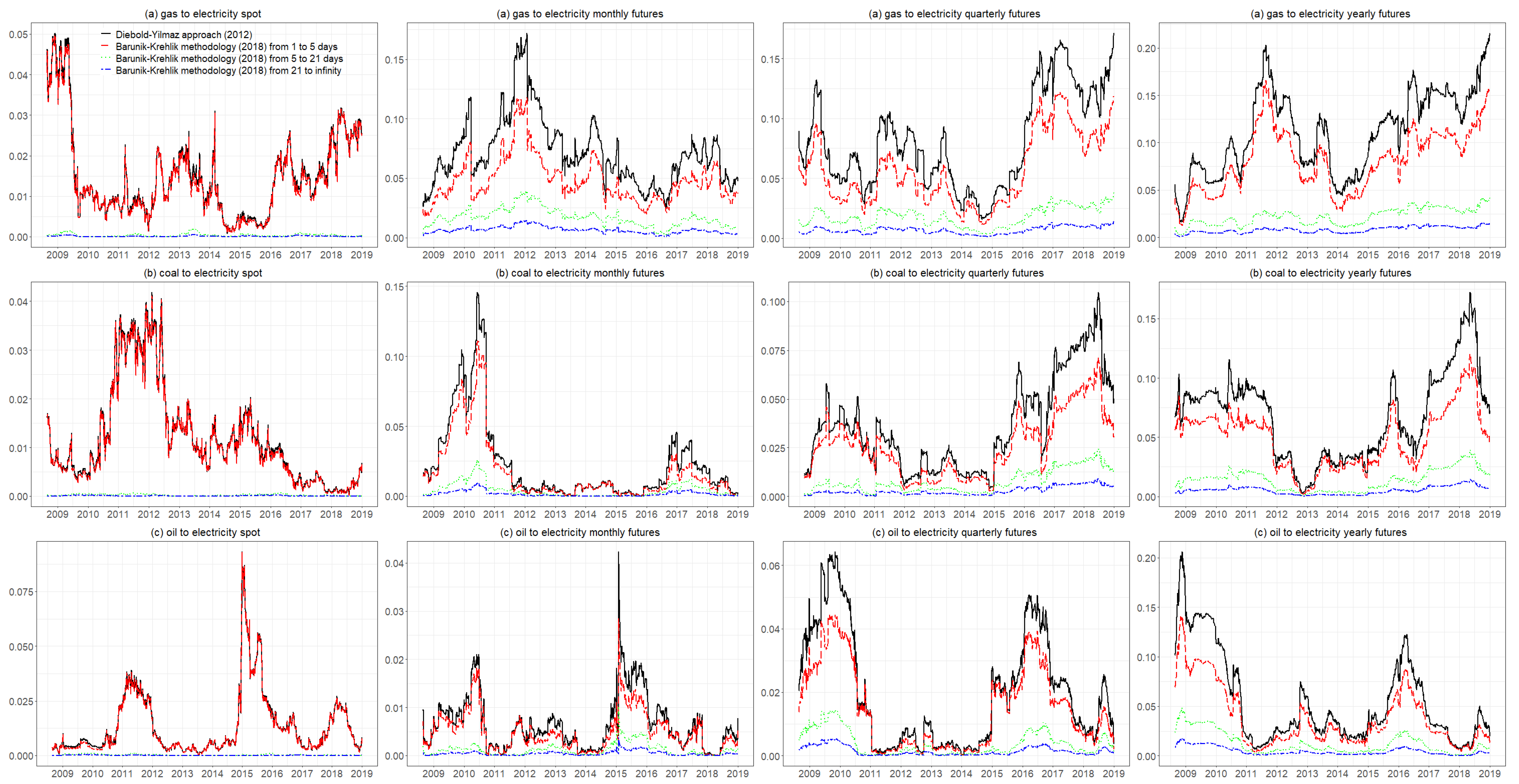
Figure A1.
Diebold–Yilmaz approach (2012) directional return spillover (Pairwise) and Barunik–Krehlik methodology (2018) directional return spillover (Pairwise).
Figure A1.
Diebold–Yilmaz approach (2012) directional return spillover (Pairwise) and Barunik–Krehlik methodology (2018) directional return spillover (Pairwise).

Figure A2.
Diebold–Yilmaz approach (2012) directional volatility spillover (Pairwise) and Barunik–Krehlik methodology (2018) directional volatility spillover (Pairwise).
Figure A2.
Diebold–Yilmaz approach (2012) directional volatility spillover (Pairwise) and Barunik–Krehlik methodology (2018) directional volatility spillover (Pairwise).

References
- Bublitz, A.; Keles, D.; Fichtner, W. An analysis of the decline of electricity spot prices in Europe: Who is to blame? Energy Policy 2017, 107, 323–336. [Google Scholar] [CrossRef]
- Kalantzis, F.G.; Milonas, N.T. Analyzing the impact of futures trading on spot price volatility: Evidence from the spot electricity market in France and Germany. Energy Econ. 2013, 36, 454–463. [Google Scholar] [CrossRef]
- Menezes, L.M.; Houllier, M.A.; Tamvakis, M. Time-varying convergence in European electricity spot markets and their association with carbon and fuel prices. Energy Policy 2016, 88, 613–627. [Google Scholar] [CrossRef]
- Paschen, M. Dynamic analysis of the German day-ahead electricity spot market. Energy Econ. 2016, 59, 118–128. [Google Scholar] [CrossRef] [Green Version]
- Huisman, R.; Kilic, M. Electricity futures prices: Indirect storability, expectations, and risk Premiums. Energy Econ. 2012, 34, 892–898. [Google Scholar] [CrossRef]
- Islyaev, S.; Date, P. Electricity futures price models: Calibration and forecasting. Eur. J. Oper. Res. 2015, 247, 144–154. [Google Scholar] [CrossRef] [Green Version]
- Junttila, J.; Myllymäki, V.; Raatikainen, J. Pricing of electricity futures based on locational price differences: The case of Finland. Energy Econ. 2018, 71, 222–237. [Google Scholar] [CrossRef]
- Kallabis, T.; Pape, C.; Weber, C. The plunge in German electricity futures prices Analysis using a parsimonious fundamental model. Energy Policy 2016, 95, 280–290. [Google Scholar] [CrossRef]
- BP Statistical Review of World Energy. Available online: https://www.bp.com/en/global/corporate/energy-economics/statistical-review-of-world-energy.html (accessed on 15 August 2019).
- Mosquera-López, S.; Nursimulu, A. Drivers of electricity price dynamics: Comparative analysis of spot and futures markets. Energy Policy 2019, 126, 76–87. [Google Scholar] [CrossRef]
- Emery, G.W.; Liu, Q.F. An analysis of the relationship between electricity and natural-gas futures prices. J. Futures Mark. 2002, 22, 95–122. [Google Scholar] [CrossRef]
- Mjelde, J.W.; Bessler, D.A. Market integration among electricity markets and their major fuel source markets. Energy Econ. 2009, 31, 482–491. [Google Scholar] [CrossRef]
- Furió, D.; Chuliá, H. Price and volatility dynamics between electricity and fuel costs: Some evidence for Spain. Energy Econ. 2012, 34, 2058–2065. [Google Scholar] [CrossRef]
- Serletis, A.; Shahmoradi, A. Measuring and Testing Natural Gas and Electricity Markets Volatility: Evidence from Alberta’s Deregulated Markets. Stud. Nonlinear Dyn. Econ. 2006, 10, 1–20. [Google Scholar] [CrossRef]
- Green, R.; Larsson, K.; Lunina, V.; Nilsson, B. Cross-commodity news transmission and volatility spillovers in the German energy markets. Bank. Financ. 2018, 95, 231–243. [Google Scholar] [CrossRef] [Green Version]
- Diebold, F.X.; Yilmaz, K. Measuring financial asset return and volatility spillovers, with application to global equity markets. Econ. J. 2009, 119, 158–171. [Google Scholar] [CrossRef] [Green Version]
- Diebold, F.X.; Yilmaz, K. Better to give than to receive: Forecast-based measurement of volatility spillovers. Int. J. Forecast. 2012, 28, 57–66. [Google Scholar] [CrossRef] [Green Version]
- Baruník, J.; Křehlík, T. Measuring the frequency dynamics of financial connectedness and systemic risk. J. Financ. Econ. 2018, 16, 271–296. [Google Scholar] [CrossRef]
- Singh, V.K.; Nishant, S.; Kumar, P. Dynamic and directional network connectedness of crude oil and currencies: Evidence from implied volatility. Energy Econ. 2018, 76, 48–63. [Google Scholar] [CrossRef]
- Kang, S.H.; Lee, J.W. The network connectedness of volatility spillovers across global futures markets. Phys. A. Stat. Mech. Its Appl. 2019, 526, 120756. [Google Scholar] [CrossRef]
- Malik, F.; Umar, Z. Dynamic connectedness of oil price shocks and exchange rates. Energy Econ. 2019. [Google Scholar] [CrossRef]
- Lovcha, Y.; Perez-Laborda, A. Dynamic frequency connectedness between oil and natural gas volatilities. Econ. Model. 2019. [Google Scholar] [CrossRef]
- Lau, M.C.K.; Vigne, S.A.; Wang, S.X.; Yarovaya, L. Return spillovers between white precious metal ETFs: The role of oil, gold, and global equity. Int. Rev. Financ. Anal. 2017, 52, 316–332. [Google Scholar] [CrossRef] [Green Version]
- Koop, G.; Pesaran, M.H.; Potter, S.M. Impulse response analysis in nonlinear multivariate models. J. Econ. 1996, 74, 119–147. [Google Scholar] [CrossRef]
- Pesaran, H.H.; Shin, Y. Generalized Impulse Response Analysis in Linear Multivariate Models. Econ. Lett. 1998, 58, 17–29. [Google Scholar] [CrossRef]
- Diebold, F.X.; Yilmaz, K. On the Network Topology of Variance Decompositions: Measuring the Connectedness of Financial Firms. J. Econ. 2014, 182, 119–134. [Google Scholar] [CrossRef] [Green Version]
- Toyoshima, Y.; Hamori, S. Measuring the Time-Frequency dynamics of return and volatility connectedness in global crude oil markets. Energies 2018, 11, 2893. [Google Scholar] [CrossRef] [Green Version]
- Fama, E.F.; French, K.R. Commodity future prices: Some evidence on forecast power, premiums, and the theory of storage. J. Bus. 1987, 60, 55–73. [Google Scholar] [CrossRef]
Figure 1.
Time-variations of the price series. Note: spot: EPEX Germany Baseload Spot; monthly futures: EEX Germany Baseload Monthly Futures; quarterly futures: EEX Germany Baseload Quarterly Futures; yearly futures: EEX Germany Baseload Yearly Futures; gas: ICE UK Natural Gas Monthly Futures; coal: ICE Rotterdam Coal Monthly Futures; oil: ICE Brent Crude Oil Monthly Futures; the units of electricity spot, monthly futures, quarterly futures, and yearly futures are EUR/Mwh; the units of gas, coal, oil are EUR/therm, EUR/metric ton, and EUR/barrel, respectively.

Figure 2.
Diebold–Yilmaz approach (2012) directional return spillover (From) and Barunik–Krehlik methodology (2018) directional return spillover (From). Note: spot: EPEX Germany Baseload Spot; monthly futures: EEX Germany Baseload Monthly Futures; quarterly futures: EEX Germany Baseload Quarterly Futures; yearly futures: EEX Germany Baseload Yearly Futures.


Figure 3.
Electricity generation by natural gas in Europe. Data source: BP Statistical Review of World Energy, 2019.
Figure 3.
Electricity generation by natural gas in Europe. Data source: BP Statistical Review of World Energy, 2019.

Figure 4.
Diebold–Yilmaz approach (2012) directional volatility spillover (From) and Barunik–Krehlik methodology (2018) directional volatility spillover (From). Note: spot: EPEX Germany Baseload Spot; monthly futures: EEX Germany Baseload Monthly Futures; quarterly futures: EEX Germany Baseload Quarterly Futures; yearly futures: EEX Germany Baseload Yearly Futures.


Table 1.
The spillover table of the Diebold–Yilmaz approach (2012).
| Spillover Results | |||||
|---|---|---|---|---|---|
| … | From others | ||||
| … | |||||
| … | |||||
| … | |||||
Note: adapted from “On the Network Topology of Variance Decompositions: Measuring the Connectedness of Financial Firms” [26].
Table 2.
The spillover table of the Barunik–Krehlik methodology (2018).
| Spillover Results | |||||
|---|---|---|---|---|---|
| … | From others | ||||
| … | |||||
| … | |||||
| … | |||||
Note: adapted from “On the Network Topology of Variance Decompositions: Measuring the Connectedness of Financial Firms” [26].
Table 3.
Variables in the model.
| Variable | Data | Data Source |
|---|---|---|
| Ele_Spot | EPEX Germany Baseload Spot | Bloomberg |
| Ele_Fut_Mon | EEX Germany Baseload Monthly Futures | Bloomberg |
| Ele_Fut_Qr | EEX Germany Baseload Quarterly Futures | Bloomberg |
| Ele_Fut_Yr | EEX Germany Baseload Yearly Futures | Bloomberg |
| Gas | ICE UK Natural Gas Monthly Futures | Bloomberg |
| Coal | ICE Rotterdam Coal Monthly Futures | Bloomberg |
| Oil | ICE Brent Crude Oil Monthly Futures | Bloomberg |
Table 4.
Descriptive statistics of the return and volatility series.
| Spot | Fut_Mon | Fut_Qr | Fut_Yr | Gas | Coal | Oil | |
|---|---|---|---|---|---|---|---|
| Descriptive Statistics of the Return | |||||||
| Mean | 0.0002 | 0.0000 | 0.0001 | −0.0000 | 0.0001 | 0.0001 | 0.0000 |
| Minimum | −2.0000 | −0.2429 | −0.2002 | −0.09366 | −0.1334 | 0.2179 | −0.1094 |
| Maximum | 2.3785 | 0.4042 | 0.3422 | 0.1535 | 0.3589 | 0.1751 | 0.1718 |
| Std. Dev. | 0.2537 | 0.0315 | 0.0204 | 0.0118 | 0.0296 | 0.0161 | 0.0211 |
| Skewness | 0.6253 | 2.415 | 3.1200 | 0.5691 | 1.8429 | −0.4293 | 0.0590 |
| Kurtosis | 11.4001 | 38.3887 | 72.8856 | 16.7734 | 22.1089 | 35.6286 | 7.3911 |
| JB | 9072.9 *** | 160,472 *** | 619,264 *** | 24,026 *** | 47,642 *** | 134,014 *** | 2427.2 *** |
| ADF | −56.9 *** | −37.7 *** | −36.9 *** | −38.0 *** | −39.8 *** | −39.1 *** | −39.9 *** |
| PP | −123.9 *** | −52.1 *** | −51.6 *** | −50.9 *** | −52.2 *** | −53.2 *** | −59.1 *** |
| Descriptive Statistics of the Volatility | |||||||
| Mean | 0.0589 | 0.0010 | 0.0003 | 0.0001 | 0.0001 | 0.0003 | 0.0004 |
| Minimum | 0.0160 | 0.0006 | 0.0000 | 0.0000 | 0.0009 | 0.0001 | 0.0001 |
| Maximum | 0.9180 | 0.0020 | 0.0068 | 0.0023 | 0.0136 | 0.0018 | 0.0048 |
| Std. Dev. | 0.0589 | 0.0003 | 0.0005 | 0.0002 | 0.0012 | 0.0002 | 0.0005 |
| Skewnesss | 5.3783 | 1.3262 | 6.3463 | 4.0463 | 4.0977 | 2.9271 | 3.5460 |
| Kurtosis | 52.2126 | 4.0317 | 58.6978 | 30.5627 | 29.5249 | 12.4334 | 20.0091 |
| JB | 319,207 *** | 1018.8 *** | 410,502 *** | 103,802 *** | 96,952 *** | 15,505 *** | 42,720 *** |
| ADF | −9.7 *** | −3.4 ** | −10.3 *** | −5.6 *** | −7.0 *** | −3.0 ** | −3.5 *** |
| PP | −11.7 *** | −3.3 ** | −12.6 *** | −7.8 *** | −10.2 *** | −3.3 ** | −3.9 *** |
Note: Spot, Fut_Mon, Fut_Qr, Fut_Yr, Gas, Coal, Oil refer to EPEX Germany Baseload Spot, EEX Germany Baseload Monthly Futures, EEX Germany Baseload Quarterly Futures, EEX Germany Baseload Yearly Futures, ICE UK Natural Gas Monthly Futures, ICE Rotterdam Coal Monthly Futures, ICE Brent Crude Oil Monthly Futures, respectively. JB: Jarque and Bera Test (1980); ADF: Augmented Dickey and Fuller Unit Root Test (1979); PP: Phillips and Perron Unit Root Test (1988); *, ** and *** denote rejection of the null hypothesis at 10%, 5% and 1% significance levels, respectively.
Table 5.
The return spillover results of the Diebold–Yilmaz approach (2012).
| Return Spillovers | |||||
|---|---|---|---|---|---|
| Electricity Spot | |||||
| Ele_Spot | Gas | Coal | Oil | From | |
| Ele_Spot | 99.578 | 0.205 | 0.118 | 0.099 | 0.106 |
| Electricity Monthly Futures | |||||
| Ele_Fut_Mon | Gas | Coal | Oil | From | |
| Ele_Fut_Mon | 93.738 | 4.549 | 1.348 | 0.364 | 1.565 |
| Electricity Quarterly Futures | |||||
| Ele_Fut_Qr | Gas | Coal | Oil | From | |
| Ele_Fut_Qr | 87.512 | 8.142 | 2.719 | 1.627 | 3.122 |
| Electricity Yearly Futures | |||||
| Ele_Fut_Yr | Gas | Coal | Oil | From | |
| Ele_Fut_Yr | 77.674 | 10.015 | 7.176 | 5.136 | 5.581 |
Note: Ele_Spot, Ele_Fut_Mon, Ele_Fut_Qr, Ele_Fut_Yr, Gas, Coal, Oil refer to EPEX Germany Baseload Spot, EEX Germany Baseload Monthly Futures, EEX Germany Baseload Quarterly Futures, EEX Germany Baseload Yearly Futures, ICE UK Natural Gas Monthly Futures, ICE Rotterdam Coal Monthly Futures, ICE Brent Crude Oil Monthly Futures, respectively.
Table 6.
The return spillover results of the Barunik–Krehlik methodology (2018).
| Return Spillovers | |||||
|---|---|---|---|---|---|
| Electricity Spot | |||||
| Frequency H 1–5 Days | |||||
| Ele_Spot | Gas | Coal | Oil | From | |
| Ele_Spot | 97.182 | 0.193 | 0.116 | 0.084 | 0.098 |
| Frequency M 5–21 Days | |||||
| Ele_Spot | 1.902 | 0.009 | 0.002 | 0.011 | 0.005 |
| Frequency L > 21 Days | |||||
| Ele_Spot | 0.494 | 0.003 | 0.001 | 0.004 | 0.002 |
| Electricity Monthly Futures | |||||
| Frequency H 1–5 Days | |||||
| Ele_Fut_Mon | Gas | Coal | Oil | From | |
| Ele_Fut_Mon | 74.381 | 2.913 | 0.961 | 0.250 | 1.031 |
| Frequency M 5–21 Days | |||||
| Ele_Fut_Mon | 14.234 | 1.191 | 0.283 | 0.083 | 0.389 |
| Frequency L > 21 Days | |||||
| Ele_Fut_Mon | 5.123 | 0.445 | 0.104 | 0.031 | 0.145 |
| Electricity Quarterly Futures | |||||
| Frequency H 1–5 Days | |||||
| Ele_Fut_Qr | Gas | Coal | Oil | From | |
| Ele_Fut_Qr | 68.856 | 5.671 | 1.974 | 1.149 | 2.199 |
| Frequency M 5–21 Days | |||||
| Ele_Fut_Qr | 13.703 | 1.803 | 0.545 | 0.349 | 0.674 |
| Frequency L > 21 Days | |||||
| Ele_Fut_Qr | 4.953 | 0.668 | 0.200 | 0.129 | 0.249 |
| Electricity Yearly Futures | |||||
| Frequency H 1–5 Days | |||||
| Ele_Fut_Yr | Gas | Coal | Oil | From | |
| Ele_Fut_Yr | 60.862 | 7.287 | 5.117 | 3.450 | 3.964 |
| Frequency M 5–21 Days | |||||
| Ele_Fut_Yr | 12.348 | 1.993 | 1.505 | 1.231 | 1.182 |
| Frequency L > 21 Days | |||||
| Ele_Fut_Yr | 4.464 | 0.734 | 0.553 | 0.455 | 0.436 |
Note: Ele_Spot, Ele_Fut_Mon, Ele_Fut_Qr, Ele_Fut_Yr, Gas, Coal, Oil refer to EPEX Germany Baseload Spot, EEX Germany Baseload Monthly Futures, EEX Germany Baseload Quarterly Futures, EEX Germany Baseload Yearly Futures, ICE UK Natural Gas Monthly Futures, ICE Rotterdam Coal Monthly Futures, ICE Brent Crude Oil Monthly Futures, respectively.
Table 7.
The volatility spillover results of the Diebold–Yilmaz approach (2012).
| Volatility Spillovers | |||||
|---|---|---|---|---|---|
| Electricity Spot | |||||
| Ele_Spot | Gas | Coal | Oil | From | |
| Ele_Spot | 98.804 | 0.691 | 0.407 | 0.098 | 0.299 |
| Electricity Monthly Futures | |||||
| Ele_Fut_Mon | Gas | Coal | Oil | From | |
| Ele_Fut_Mon | 87.992 | 9.539 | 2.052 | 0.417 | 3.002 |
| Electricity Quarterly Futures | |||||
| Ele_Fut_Qr | Gas | Coal | Oil | From | |
| Ele_Fut_Qr | 95.585 | 3.565 | 0.639 | 0.211 | 1.104 |
| Electricity Yearly Futures | |||||
| Ele_Fut_Yr | Gas | Coal | Oil | From | |
| Ele_Fut_Yr | 88.839 | 0.145 | 9.181 | 1.835 | 2.790 |
Note: Ele_Spot, Ele_Fut_Mon, Ele_Fut_Qr, Ele_Fut_Yr, Gas, Coal, Oil refer to EPEX Germany Baseload Spot, EEX Germany Baseload Monthly Futures, EEX Germany Baseload Quarterly Futures, EEX Germany Baseload Yearly Futures, ICE UK Natural Gas Monthly Futures, ICE Rotterdam Coal Monthly Futures, ICE Brent Crude Oil Monthly Futures, respectively.
Table 8.
The volatility spillover results of the Barunik–Krehlik methodology (2018).
| Volatility Spillovers | |||||
|---|---|---|---|---|---|
| Electricity Spot | |||||
| Frequency H 1–5 Days | |||||
| Ele_Spot | Gas | Coal | Oil | From | |
| Ele_Spot | 9.671 | 0.003 | 0.003 | 0.002 | 0.002 |
| Frequency M 5–21 Days | |||||
| Ele_Spot | 35.053 | 0.042 | 0.009 | 0.010 | 0.015 |
| Frequency L > 21 Days | |||||
| Ele_Spot | 54.079 | 0.646 | 0.395 | 0.086 | 0.282 |
| Electricity Monthly Futures | |||||
| Frequency H 1–5 Days | |||||
| Ele_Fut_Mon | Gas | Coal | Oil | From | |
| Ele_Fut_Mon | 0.297 | 0.009 | 0.010 | 0.009 | 0.007 |
| Frequency M 5–21 Days | |||||
| Ele_Fut_Mon | 0.852 | 0.029 | 0.029 | 0.026 | 0.021 |
| Frequency L > 21 Days | |||||
| Ele_Fut_Mon | 86.843 | 9.502 | 2.012 | 0.382 | 2.974 |
| Electricity Quarterly Futures | |||||
| Frequency H 1–5 Days | |||||
| Ele_Fut_Qr | Gas | Coal | Oil | From | |
| Ele_Fut_Qr | 9.962 | 0.195 | 0.000 | 0.014 | 0.052 |
| Frequency M 5–21 Days | |||||
| Ele_Fut_Qr | 24.567 | 0.536 | 0.001 | 0.034 | 0.143 |
| Frequency L > 21 Days | |||||
| Ele_Fut_Qr | 61.057 | 2.834 | 0.638 | 0.164 | 0.909 |
| Electricity Yearly Futures | |||||
| Frequency H 1–5 Days | |||||
| Ele_Fut_Yr | Gas | Coal | Oil | From | |
| Ele_Fut_Yr | 4.405 | 0.002 | 0.018 | 0.001 | 0.005 |
| Frequency M 5–21 Days | |||||
| Ele_Fut_Yr | 11.985 | 0.005 | 0.050 | 0.003 | 0.015 |
| Frequency L > 21 Days | |||||
| Ele_Fut_Yr | 72.448 | 0.138 | 9.113 | 1.831 | 2.771 |
Note: Ele_Spot, Ele_Fut_Mon, Ele_Fut_Qr, Ele_Fut_Yr, Gas, Coal, Oil refer to EPEX Germany Baseload Spot, EEX Germany Baseload Monthly Futures, EEX Germany Baseload Quarterly Futures, EEX Germany Baseload Yearly Futures, ICE UK Natural Gas Monthly Futures, ICE Rotterdam Coal Monthly Futures, ICE Brent Crude Oil Monthly Futures, respectively.
© 2020 by the authors. Licensee MDPI, Basel, Switzerland. This article is an open access article distributed under the terms and conditions of the Creative Commons Attribution (CC BY) license (http://creativecommons.org/licenses/by/4.0/).
Share and Cite
MDPI and ACS Style
Liu, T.; He, X.; Nakajima, T.; Hamori, S. Influence of Fluctuations in Fossil Fuel Commodities on Electricity Markets: Evidence from Spot and Futures Markets in Europe. Energies 2020, 13, 1900. https://doi.org/10.3390/en13081900
AMA Style
Liu T, He X, Nakajima T, Hamori S. Influence of Fluctuations in Fossil Fuel Commodities on Electricity Markets: Evidence from Spot and Futures Markets in Europe. Energies. 2020; 13(8):1900. https://doi.org/10.3390/en13081900
Chicago/Turabian StyleLiu, Tiantian, Xie He, Tadahiro Nakajima, and Shigeyuki Hamori. 2020. "Influence of Fluctuations in Fossil Fuel Commodities on Electricity Markets: Evidence from Spot and Futures Markets in Europe" Energies 13, no. 8: 1900. https://doi.org/10.3390/en13081900
Note that from the first issue of 2016, this journal uses article numbers instead of page numbers. See further details here.