Application of Multivariate Statistical Methods and Artificial Neural Network for Facies Analysis from Well Logs Data: an Example of Miocene Deposits


Department of Geophysics, Faculty of Geology, Geophysics and Environmental Protection, AGH University of Science and Technology, Mickiewicza 30, 30-059 Krakow, Poland
Energies 2020, 13(7), 1548; https://doi.org/10.3390/en13071548
Submission received: 12 February 2020
/
Revised: 13 March 2020
/
Accepted: 20 March 2020
/
Published: 26 March 2020
Abstract
:The main purpose of the study is a detailed interpretation of the facies and relate these to the results of standard well logs interpretation. Different methods were used: firstly, multivariate statistical methods, like principal components analysis, cluster analysis and discriminant analysis; and secondly, the artificial neural network, to identify and discriminate the facies from well log data. Determination of electrofacies was done in two ways: firstly, analysis was performed for two wells separately, secondly, the neural network learned and trained on data from the W-1 well was applied to the second well W-2 and a prediction of the facies distribution in this well was made. In both wells, located in the area of the Carpathian Foredeep, thin-layered sandstone-claystone formations were found and gas saturated depth intervals were identified. Based on statistical analyses, there were recognized presence of thin layers intersecting layers of much greater thickness (especially in W-2 well), e.g., section consisting mainly of claystone and sandstone formations with poor reservoir parameters (Group B) is divided with thin layers of sandstone and claystone with good reservoir parameters (Group C). The highest probability of occurrence of hydrocarbons exists in thin-layered intervals in facies C.
1. Introduction
Interpretation of well logging data is an important stage in research related to the exploration and recognition of oil and natural gas deposits. In the era of widely developed possibilities of processing and interpreting measurements of well logging data, statistical methods are an easy and inexpensive tool to support data analysis. The availability of statistical programs enables fast and effective interpretation of the well logging data.
Identifying facies is an important element of petroleum prospecting and reservoir characterization. High precision of facies prediction is one of the key step for the construction geologically justified, static reservoir models. Usually, identification of sedimentary facies is based on both qualitative and quantitative parameters, including mineral composition, pore/grain size distribution, texture, stratification, sedimentary structures and bioturbation. A lithofacies can be defined as a stratigraphic units, that can be distinguishable from the adjacent beds based on the lithological characteristics such as mineralogical, petrographic and paleontological signatures associated with the appearance, texture or composition of the rock. They were deposited in a similar environment and have a similar diagenetic history [1].
Well logs data do not contain enough information to define all lithofacies features, as they may include biological and other features not identified by logs. They can determine a subset of ‘facies’ which in this paper will be called electrofacies. That term was first used by Serra and Abbott in 1981 [2], to define the set of log responses which characterizes a bed and permits this to be distinguished from others. Electrofacies can usually be assigned to one or more lithofacies as log responses are measurements of the physical properties of rocks. Facies distributions based on well logs are highly desirable, as they represent the most abundant and widespread dataset in subsurface studies. The process of quantitatively determining facies from well logs is currently being improved so that it can be applied in various sedimentary basins and deposits from different depositional environments [3,4,5].
From the years researchers have focused on using statistical methods and machine learning algorithms to analyse facies from well logs, due to their ability to resolve non-linear relationships, quantify learning from training data, and work in conjunction with other kinds of artificial intelligence [3,4,6,7,8]. Advanced statistical models have been introduced to automate the task of facies identification. These include methods such as non-parametric regression, factor analysis, principal component analysis, classification trees, clustering and techniques based on machine learning and artificial intelligence [9,10,11,12]. The electrofacies and the lithofacies are similar in attempting to identify and group rocks based on large-scale geologic and petrophysical features as shown by the log responses. Thus, the main purpose of the electrofacies identification is to correlate them with the lithofacies and to identify reservoir parameters related to them [13,14,15]. Process of classification and predicting electrofacies involves fuzziness at many levels, but the final desired result, facies class, is discrete. Discrete class boundaries that theoretically could be enforced by objective measurements are subjective and fuzzy in practice.
In this paper different methods were used: firstly, the multivariate statistical methods, like principal components analysis (PCA), cluster analysis (CA) and discriminant analysis (DA); and secondly, the artificial neural network (ANN) to identification and discrimination the facies from well log data. The main purpose of the study is a detailed interpretation of the electrofacies and relate these to the results of standard well logs interpretation.
To predict and analyse electrofacies, two software packages were used: TechLog, from Schlumberger software [16] and Statistica from Statsoft [17]. As a testing data set the Miocene-age sandy–shaly formations in the Carpathian Foredeep in Poland were used.
The experiment involved the following steps:
- Prepare data in pre-processing;
- Statistical data analysis (PCA, CA, DA);
- Design, train and test classifiers (ANN);
- Facies prediction;
- Analyse and compare results.
Determination of electrofacies was done in two ways:
- 1)
- In the first step, analysis was performed for each well separately;
- 2)
- in the second stage, the neural network taught on data from the W-1 well was applied to the second well and a prediction of the facies distribution in this well was made.
2. Materials and Methods
2.1. Well Log Measurements
Well logs that were used for facies identification and prediction included gamma-ray (GR [API]), spectral gamma-ray without uranium content (GRKT [API]), bulk density (RHOB [g/cc]), transit interval time (DT [μs/m]), neutron porosity (NPHI [% ls]), deep resistivity (LLD [ohm·m]), shallow resistivity (LLS [ohm·m]), photoelectric factor (PE [b/el.]) and calliper CALI [mm]). Data series are composed of about 3000 points sampled at intervals of 10 cm. Two intervals from two wells (W-1 well–depth interval from 1250 to 1400 m, W-2 well depth interval from 1350 to 1500 m) was taken into account during the analysis.
To handle with a facies identification and prediction, set of well logs should contain useful information about lithology and reservoir parameters. GR provides an information about the natural radioactivity of the rocks, reflecting clay content since radioactive elements tend to concentrate in clay minerals; GRKT exclude the uranium (uranium can be also present in organic matter) content from the total radioactivity; RHOB provides information of a bulk density of rocks; PE can be treated as a lithology factor; DT logs measure interval transit time of a travelling of a compressional wave through the formation and NPHI reacts on the presence of hydrogen. LLD and LLS measure resistivity from the virgin and filtration zone and is a reflection of the pore space saturation.
2.2. Data Descriptions
The Carpathian Foredeep is a peripheral molasses sedimentary basin formed on the outskirts of the Carpathian Mountains. During the Paleogene, all this area was uplifted and intensely eroded. Base of foredeep is epivariscan platform and Permian-Mesozoic, Miocene-age formations lie above. The Miocene structural complex is the most important one in the geological pattern of the Carpathian Foredeep. Miocene sediments, located in the eastern part of the Carpathian Foredeep, were formed in the northern part of the post-orogenic basin. There are external and internal parts. Their filling are Miocene deposits, with some of these sediments remaining intact (Miocene autochthonic sediments), and some have been rooted, folded together with the Carpathian folds and moved north to autochthonic sediments [18,19].
Area of research is located in the east part of Carpathian Foredeep Basin in south-east Poland, contain heterolithic Miocene-age deposits. Statistical analyses were performed for data from the W-1 and W-2 wells at selected 150 m thick depth intervals. Selected depth intervals in both wells correspond to each other in lithological and sedimentological parameters. At selected intervals, the presence of gas was observed: in significant quantities (W-1) and to a small extent (W-2). Intervals subjected to statistical analysis are built mainly of Miocene-age sandstones, claystones and mudstones. Both wells were drilled through similar rock formations, conducive to the formation of structural and stratigraphic traps in which hydrocarbons are accumulated.
2.3. Principal Component Analysis (PCA)
Principal Component Analysis is a method of data analysis, based on mathematical operation, consisting in transforming a set of observations, most often correlated variables, into a set of values of uncorrelated variables, called the main components [20]. This method finds sequences of linear combinations between variables with maximum variance and a low correlation coefficient. By reducing the number of variables, analysis of the main components also facilitates data visualization. Main component analysis results are used in regression calculations and for cluster analysis.
The idea of analysing the main components is to transform the output set of variables X1, … Xp into a new set of variables Z1, … Zp. The new variables Z1, … Zp are called the principal components. To maintain the highest data variability, the first principal component Z1 should have maximum variance. This means that the values of weighting factors should assume such that the value of the main component variance Z1 is as high as possible. In other words, the first principal component is an eigenvector corresponding to the largest eigenvalue of the X1, … Xp covariance matrix. The next main components are also linear combinations of real variables, however, the explained variance is smaller than the first component. The second component meets the condition of normalization of the coefficients and the condition of orthogonality of the vectors of the first and second main components. The next main components are mutually uncorrelated. Based on the calculated eigenvalues, eigenvectors are calculated, corresponding to the eigenvalues found for all major components. To reduce the number of main components, available criteria, e.g., Kaiser or graphical, should be used [21].
2.4. Cluster Analysis (CA)
2.4.1. Hierarchical Cluster Analysis (HCA)
The hierarchical cluster analysis (HCA) method is developed for the purpose of clustering dominant electrofacies hidden in the studied reservoir (in the row data) [14,22,23,24]. This method classifies a dataset into homogeneous groups of data (electrofacies here).
The method is performed through three main steps:
- The similarity between the two samples is measured based on their distance. To calculate this parameter several metrics can be used, among which the Euclidean is more popular.
- The objects are linked together until one cluster is established. In this step, each object is considered as its cluster.
- To link objects together, based on different variables, various algorithms, such as single linkage, complete linkage, average linkage, median linkage and Ward linkage can be used. For this purpose, the last is preferred here [25].
2.4.2. K-mean Clustering
Non-hierarchical method of data clustering. It is based on grouping objects by distance, but at the beginning, objects are assigned to clusters randomly. Then the centres of gravity of randomly created clusters are calculated and the distances of objects to these centres of gravity are re-calculated. The algorithm is repeated until the objects stop moving between the clusters [14,22,23,24].
2.4.3. Discriminant Analysis (DA)
Discriminant analysis is a statistical technique that allows you to study differences between two or more groups by analysing several variables at the same time. As a result of discriminant analysis, having a set of several variables, you can distinguish one group from another. It is possible to check to what extent discriminatory variables distinguish group data and which of them best discriminate against a given set [26,27]. Conducting a proper discriminant analysis requires the determination of canonical discriminatory functions that separate groups. Discriminant function coefficients indicate how strong the impact of a given discriminant variable is on group differentiation. A higher value of the discriminant function coefficient indicates a stronger discriminatory effect of a given variable [28].
2.5. Artificial Neural Network (ANN)
Neural networks are a very sophisticated modelling technique, capable of mapping extremely complex functions and relationships. They have the unique ability to find meaning, rules and trends in complex structures of noisy and imprecise data. Also, they can be used to detect hidden patterns and dependencies controlled by such complicated functions that it would be very difficult or impossible to make a model using simple analytical methods. Neural networks can be also used for missing data prediction [29,30]. Neural networks have the basic ability to generalize, based on the fact that once taught on a certain set of data they can apply the acquired knowledge to completely new data with the same structure.
Artificial neural networks can be a great calculation tool. Networks can acquire all their knowledge from the learning process. Only adequate network complexity is required to develop appropriate connections and structures in the learning process. A network with too few elements will not be able to learn anything [31,32]. In practice, neural networks themselves construct the models needed by the user, because they automatically learn from the examples given by him. Based on this self-created data structure, the network then performs all functions related to the operation of the created model. The neurons are connected, and connections are assigned weights determined in the learning process. The connection diagram and their weights constitute the network’s program of operation, while the signals appearing at the output are solutions to its tasks.
Neural networks are also used in classification tasks. In that case, the answer is one of the given categories. For example, if all data samples fall into one of three categories, then the network will classify each sample into one of these three classes. Information about the belonging of a data case to a particular class is contained in the output variable t. Therefore, in the analysis of a classification problem, the output variable is always categorized, that means one that accepts a finite number of values that are not sorted.
Kohonen Algorithm
SOM, also called topological ordered maps, or Kohonen self-organizing feature map (KSOM) is the neural network learning without supervisor to maps all the points in a high-dimensional source space into a 2 to 3-d target space, the distance and proximity relationship (i.e., topology) are preserved as much as possible [33]. The Kohonen network stands out from other networks in that it preserves the mapping of the neighbourhood of the input space. The result of the network operation is the classification of space in a way that groups both cases from the learning set and all other introductions after the learning process.
Cluster centres tend to lie in a low dimensional manifold in the feature space. Clustering is performed by having several units competing for the current object. The unit whose weight vector is closest to the current object wins. SOM learning consists in the fact that for each input vector the winner and his neighbours (more precisely their model vectors) are modified so that they are more similar to the presenting vector.
Having a sample x from the training set X in a given step t of the learning phase we find the map element closest to the presenting vector c (x):
After finding this element, the winner and his neighbours are modified using the formula:
where —is a function of neighbourhoods and has a smoothing effect on the elements of the grid
located in the vicinity of the winner; and t is a time variable.
The neighbourhood function is taken as a function of the Gaussian distribution:
where: is described as learning speed.
The selection of the activation function depends on the problem faced by the neural network. In multi-layer neural networks, nonlinear functions are most commonly used, since neurons with such properties have the greatest learning ability. The principle of operation of the activation function is smooth mapping of the relationship between the input and output of the network. This allows the network output to receive a value between 0 and 1 corresponding to information in the form YES–NO. Activation functions must have properties such as: easy calculation and continuity of the derivative, continuous transition between 0 and 1, and the ability to enter a parameter, characterizing the curve shape, into the argument of the function. The neuron activation functions can have different types, e.g., linear, logistic (sigmoid), tangent hyperbolic, exponential. The error function is a measure of the compliance of the network prediction with the set value. It is used to determine the magnitude of the necessary changes in neuron weights in each iteration. The error functions used to learn neural networks should give some measure of the distance between the prediction and the actual value at a given point in the input variable space. It is therefore natural to use the sum of squares of differences as a function of the error:
3. Results
3.1. Pre-processing
Several quality-assurance steps were performed on well logs before the statistical analysis:
- Checking data continuity and the uniformity of the sampling step for all logs;
- applying the required environmental corrections before identifying and processing the electrofacies;
- combining logs from measurements from other intervals and depth shifting;
- depth matching between core and well logs; it was carried out based on the correlation between core GR measurement and log-derived one;
- detecting and removing the outliers and artificial anomaly;
- normalizing variables.
3.2. PCA Results
The data obtained based on well log are a multidimensional image of the rock along the borehole. Well logs results at selected depth intervals have been normalized first. The principal components analysis was based on a correlation matrix. From the point of view of the usefulness of variables in the analysis of principal components, average correlation coefficients above 0.3 are considered significant. In the W-1 well, high correlation coefficients were observed between the resistivity values of the unchanged zone and the resistivity of the filtration zone. High correlation coefficients also occur between bulk density and both GR and GRKT. In other cases, correlations do not show significant relationships between variables. There are more relationships with a high correlation coefficient in the W-2 well. The highest correlations occur between the results of bulk density and the results from the photoelectric absorption index.
Eigenvalues were calculated based on correlation matrix of variables. The number of eigenvalues is equal to the number of input variables. Eigenvalues are ordered for percentage transferred variances from the input dataset. It is assumed that the eigenvalue of 1 corresponds to the variance carried over by one input variable. The obtained results of eigenvalues are presented in Table 1 in descending order, showing the importance of the relevant components in explaining data variability. The remaining columns present the percentage of total variance (% of total variance), cumulative eigenvalues (cumulative eigenvalue), and cumulative percent (cumulative % of variance).
As a result of the calculations, nine eigenvalues were obtained in the wells. For the data from the W-1 well, the first component corresponding to the first eigenvalue explains 46% of the total variance. Further eigenvalues explain 21% of variance and 14% of variance. In the case of data from the W-2 well, the first component corresponding to the first eigenvalue explains 62% of the total variance, the second explains 19% of the variance and third 9%. In both wells, the first main component carries the most information. Based on the Kaiser and the graphical criterion, the first three principal components were selected in both wells.
The correct interpretation of the main components is based on the value of the factor loadings. Factor loadings are the linear correlation coefficient between input variables and main components. The calculated factor loadings, presented in Table 2, confirm the selected number of main components for further interpretation. Factor loadings can be positive or negative, that means variables with opposite charges affect the same component oppositely.
W-1 well: the first PCs is built mainly of logs associated with natural radioactivity (GR, GRKT), saturation (LLS, LLD) lithology (PE) and porosity (RHOB). Factor loadings for GR and GRKT logs are −0.84 for each. RHOB and PE log with a factor load of −0.89 and −0.87, respectively. LLD and LLS logs also make a big contribution to the PC1, −0.74 each. The second main component is positively correlated with NPHI log (0.81). CALI log with a factor load of 0.75 also has a large share in the creation of the second main component. The third main component is represented mainly by DT log (0.95). The largest impact of radiometric logs in the creation of the PC1 may indicate a high shale content in the analysed depth interval. The high factor load of RHOB log indicates a significant impact of material with different bulk density. RHOB log is also a porosity indicator and is sensitive to the gas presence. It can be concluded that in that interval sandy–shaly deposits saturated with gas occur. The large contribution of information brought in by factor loadings of radiometric logs, resistivity and density may also refer to the significance of porosity and saturation parameters in the analysed interval. At the same time, a significant share of resistivity logs in the PC1 may be an important premise for the presence of gas–leading to changes in the resistance of the virgin and filtration zone. High factor loadings between PC2 and NPHI and CALI logs show a large impact of porosity and lithology on the characteristics of the analysed rocks. The highest factor load in the PC3, represented by DT log, indicates the effect of porosity in the rocks studied.
W-2 well: analysis of the main components was carried out for nine logs. As a result of the analysis, the data dimension was reduced to three main components, which explain 90% of the total variance, but the first two, explain 81% of total variance. The first main component accounts for 62% of the total variance, while the second main component accounts for 19% of the total variance (Table 2). In the third PC, only calliper log has a high impact (0.84). The next main components do not bring significant information, confirmed by high factor loadings, so only the first three main components were taken into account in the interpretation. The PC1 is built mainly of RHOB, PE, LLD, LLS, GR and GRKT logs. The PC2 is correlated with NPHI and DT logs. High factor load between the PC1 and RHOB log indicates the essence of information related to the density and porosity of rock material. The high correlation between the GR and GRKT factor load and the PC1 may indicate the presence of shales. Similarly, PE log provides a large amount of information about the lithology of the analysed interval. The high share of resistivity logs in the formation of PC1, indicates saturation changes. High values of factor loadings for DT and NPHI logs in PC2 indicate the role of porosity in the interpretation of the examined section.
3.3. CA Results
Cluster analysis was made based on row data (logs) and main components (on a new factor coordinates of the cases considered). The input data were normalized.
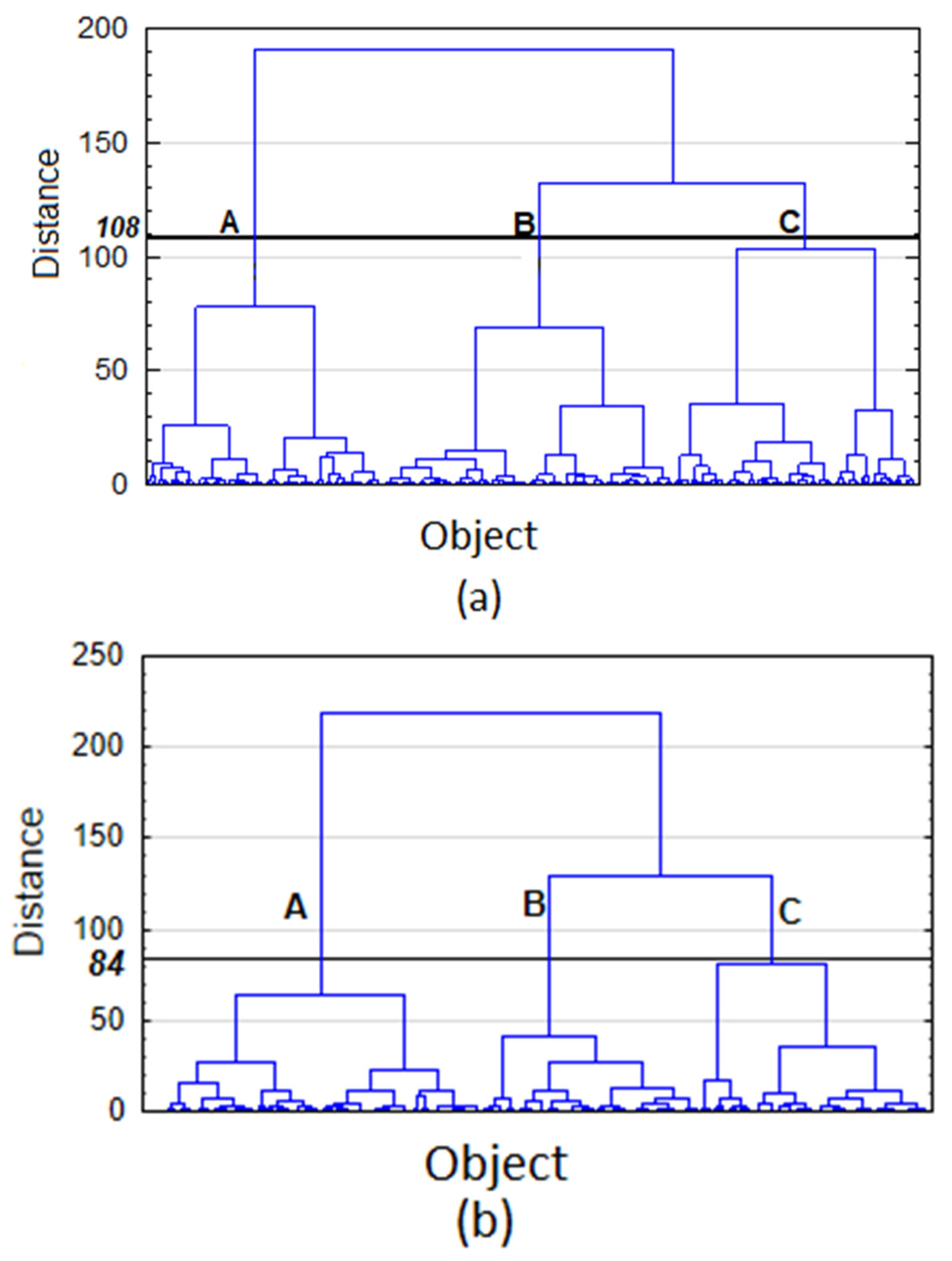
The analysis made it possible to separate clusters maximally different from each other and minimally different inside each of them. Hierarchical and k-means methods were used. In the hierarchical method, the Ward method was chosen from among the available grouping methods, which uses variance to minimize the sum of squares of deviations of any clusters that can be formed at each stage of forming [25]. To measure the distance between objects, the Euclidean distance measure was used. As a result of using hierarchical methods, dendrogram were obtained (Figure 1).
The dendrogram representing the data from the W-1 well (Figure 1a) indicates the occurrence of the three most important groups, of which two B and C are similar to each other. Similarly, the dendrogram developed based on data from the W-2 well (Figure 1b) consists of three main clusters, of which groups B and C may show similar relationships. Data from the W-1 well were divided into 3 groups: group A with 367 cases, group B with 305 cases and group C with 828 cases. Data from the W-2 well were also divided into three sets of numbers: group A–525 cases, group B–343 cases, group C–623 cases.
After conducting the hierarchical analysis and determining the number of significant groups, cluster analysis was performed using the k-means method. As a result of using the k-means method, the input data was divided into groups. According to the results of the hierarchical method, three clusters were assumed for both wells. Data from the W-1 well were divided into three groups: group A with 571 cases, group B with 663 cases and group C with 266 cases. Data from the W-2 well were also divided into three sets of numbers: group A–696 cases, group B–433 cases, group C–371 cases.
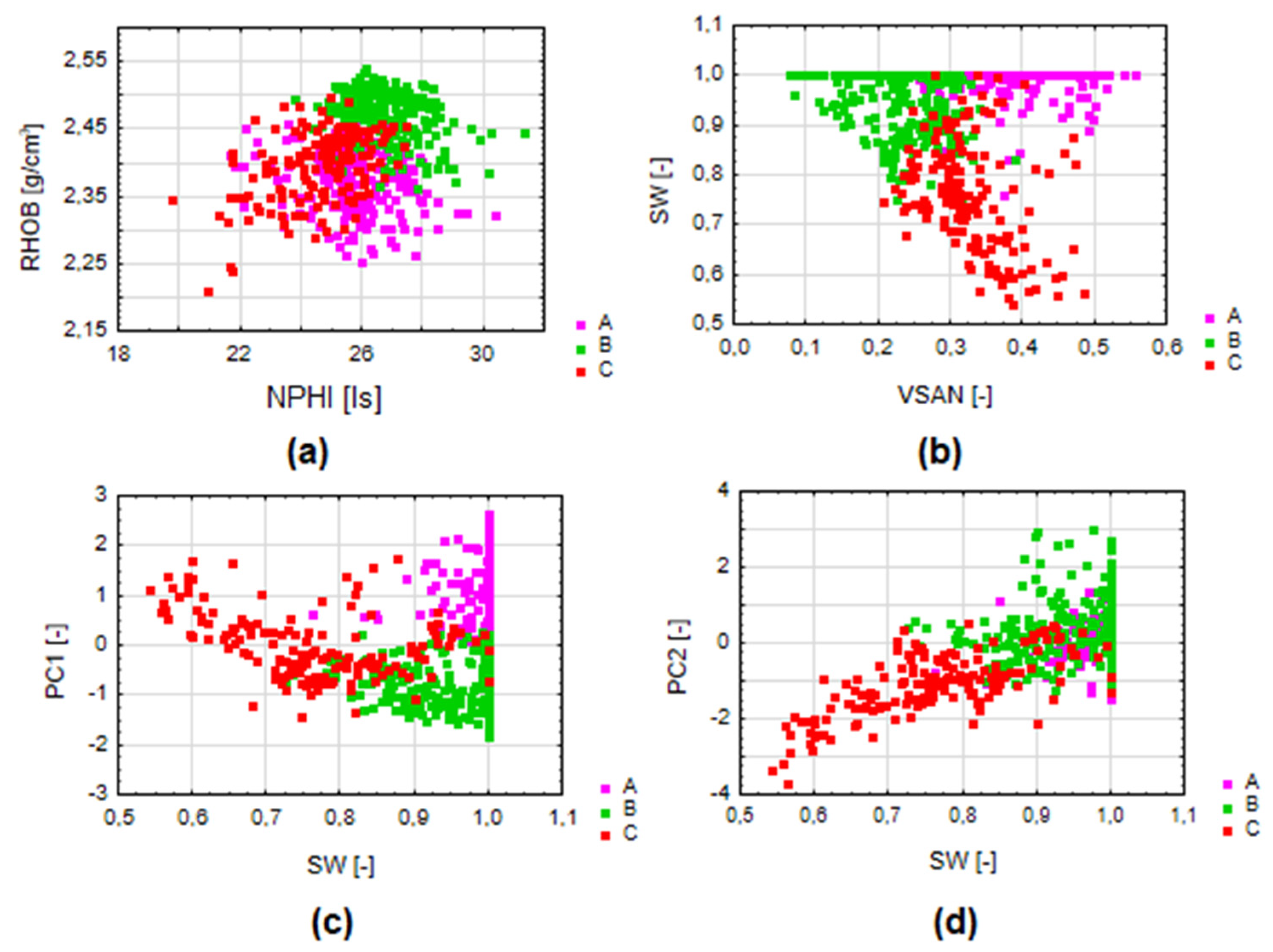
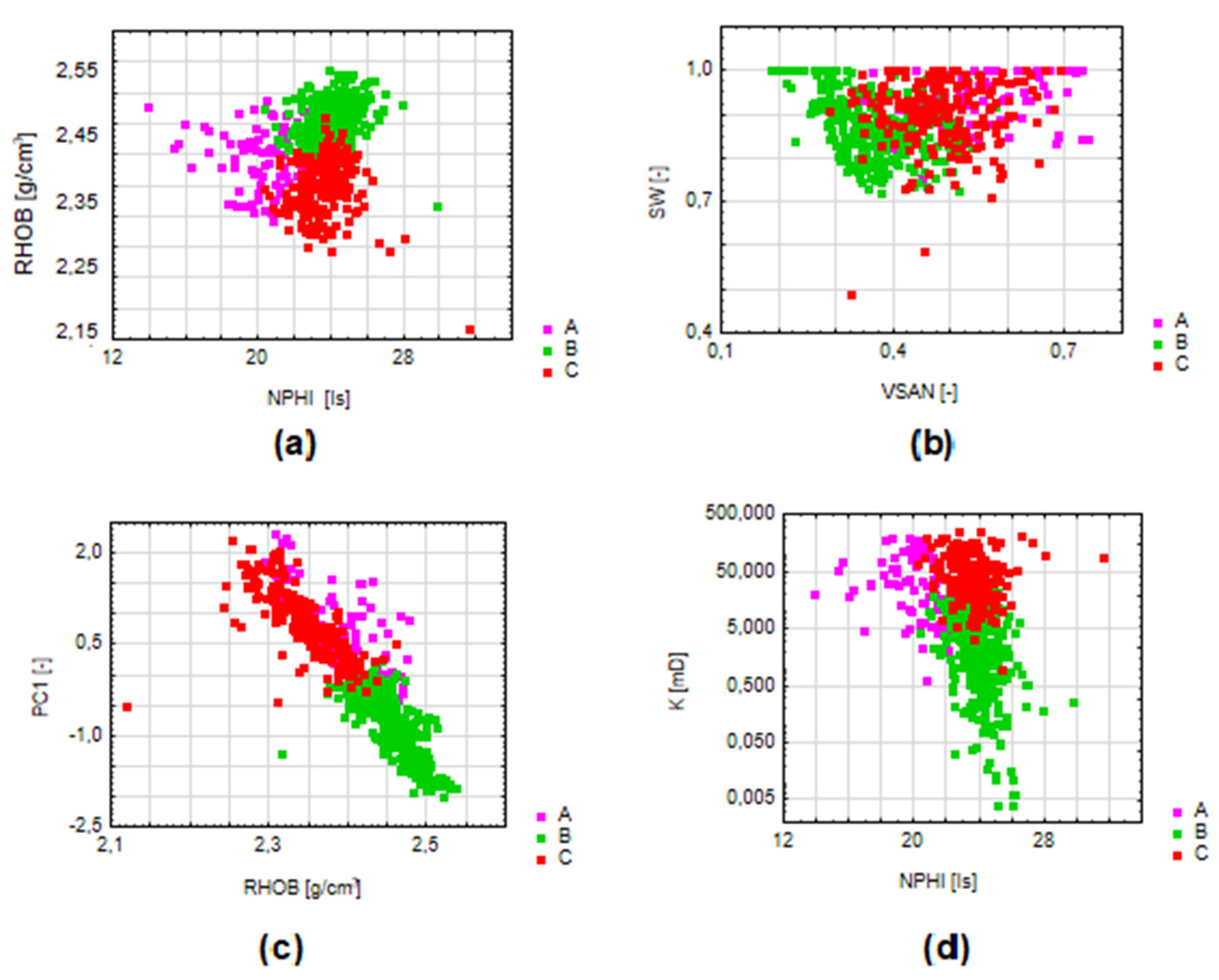
Groups (and data assign to it) were analysed in case of input data: measured logs and PCs; and the results of standard well log interpretation (SW [-]–water saturation, VSAN [-]–quartz mineral content, VCL [-]–shaliness; PHI [-]–total porosity, K [mD]–permeability), which were not taken into account during clustering. Results are shown in Figure 2 and Figure 3.
W-1 well: cluster B has the smallest total porosity PHI. We observe a high value of reservoir water saturation for data from group B and the largest volume of clay and the smallest volume of sandstones (Figure 2b). In group A, the water saturation is very high and quartz mineral volume is also very high (Figure 2b). Group C is characterized by intermediate clay and sandstone contents compared to groups A and B (Figure 2b). Group C in terms of reservoir parameters is characterized by the lowest water saturation and low porosity. The highest probability of occurrence of hydrocarbons exists in group C, due to the lowest water saturation. Groups with the highest water saturation are groups A and B. The PC1 best differentiates the designated groups in terms of saturation - a clear division into three groups (Figure 2c). On the other hand, group C was separated from the groups A and B in relation to the PC2 values (Figure 2d).
The distinguished groups A, B, C can be named as follows:
- Cluster A–sandstone-claystone deposits with poor to medium reservoir parameters (the highest water saturation, porosities in most cases do not exceed 15%);
- Cluster B–claystone-sandstone deposits with a predominance of clays, with poor reservoir parameters (high water saturation and low porosity);
- Cluster C–sandstone-claystone formations with good reservoir parameters (low water saturation and intermediate porosity values in relation to other groups).
W-2 well: in terms of clay and sand material content comparison, groups A and C are characterized by a higher content of sandstone than clay material, while in group B the situation is reversed–we observe the advantage of clay over sandstone (Figure 3b). Water saturation in all three groups has high values, with average values above 0.87. The lowest average value of water saturation occur in group B, and the highest in group A. The average porosity values in the W-2 well in the analysed section do not exceed 16%. In comparison with group B, groups A and C are characterized by increased porosity, greater water saturation and the advantage of sandstone over clay. In terms of permeability, all groups have similar values, except for group B, in which the permeability is the lowest (Figure 3d).
The distinguished groups can be named as follows:
- Cluster A–sandstone-claystone formations with poor to medium reservoir parameters (high water saturation, low porosity values);
- Cluster B–claystone-sandstone formations with poor reservoir parameters, but perspective in terms of the presence of gas (despite the lowest average water saturation and thus the probable presence of gas, there are low porosity and permeability values);
- Cluster C–sandstone-claystone formations with good reservoir parameters (low water saturation and high permeability compared to other groups).
In lithological terms of view, in both wells, there are groups with a predominance of clay material or a predominance of sandstone material. Due to such parameters as water saturation, porosity and permeability, the groups can be assigned the characteristics of good or poor reservoir parameters. From the perspective of exploratory geophysics, the most promising groups are group C in the W-1 well and next, groups B and C in the W-2 well.
3.4. DA Results
Discriminant analysis was designed to check the correctness of PCA and CA. The calculations were based on the results of the principal components analysis, i.e., factor coordinates and the results of clustering performed using the hierarchical and k-means method.
In the analysed wells, the data set was divided into two subsets: training and test set, both of different case numbers. Determination of discriminatory functions was performed on a set with a greater number of cases. Discriminant analysis was carried out for three groups A, B, C distinguished on the basis of cluster analysis. Factor coordinates of the main components were adopted as independent variables. The grouping variable is the division of cases into three groups A, B, C, highlighted during cluster analysis. For all three main components, Wilks Lambda reaches values close to zero, which indicates high discriminatory power. Similarly, the Wilks particle confirms the high discriminatory power, for all major components, it has values close to zero. In the next step, normalized coefficients of discriminant functions were calculated. The PC1 has the greatest impact on the value of the first of the discriminant functions, while for the second discriminant function the PC2. The first discriminant function accounts for 65% of the explained variance, while the second accounts for 35%. Both discriminatory functions are significant and explain a significant part of discriminatory power. Classifying functions were determined based on a priori probability for each group. Then, a classification matrix was calculated for both data sets, training and test, which describes the percentage of cases correctly classified into each group. Results of discriminant analysis are shown in Table 3.
W-1 well: In both sets, 98% of correctly qualified cases testify to the correctness of previously performed statistical analyses. The best result, 100% of correctly classified cases were obtained for group A, which determines sandstone-claystone formations with medium reservoir parameters. In the training data set, in group B the classification of cases was 99.47%. In group C, 13 observations were classified as claystone and sandstone formations with poor reservoir parameters. In the test data set, the correct classification of the data mapping to group A was also 100%, in group B, 98.08%, and in group C, 95.12%. In both collections, the best classification is in group A, representing sandstone-claystone formations with medium reservoir parameters.
W-2 well: For the training set, correct cases together constitute 96.6% of all cases, while for the test set, 94.48 % of all cases. Group B, represented by claystone-sandstone formations with poor reservoir parameters, was best qualified in both training and test sets, the correctness is equal 100%. In the training data set, 86.2% of all cases were correctly qualified for group A, while C, 95.7% of all cases were correctly classified. The correctness of classification in the test data set for groups A and C is lower for the training set and amounts to 81.82% for group A and 90.91% for group C, respectively.
Discriminant analysis confirms the correctness of statistical analyses carried out, including analysis of the main components and cluster analysis. The percentage of correctly classified cases is satisfactory for both wells. The designated groups based on statistical analyses allow the determination of lithology, saturation, porosity and permeability along the considered sections in the wells.
3.5. ANN Results
To solve task based on unsupervised approach, the Ipsom module, included in the Schlumberger Techlog software [16] was used. Ipsom module predicts and propagates rock classification groups based on neural network technology. The Ipsom module allocates points to clusters using the Kohonen algorithm. To use this module with the highest possible efficiency, a selection of properties representative of the facies is necessary. Result of using Ipsom module is output model of electrofacies and many charts and tables used to present information about model. To judge whether electrofacies from output model represent division based on petrophysical properties, the ranking variables and information table was used. Ranking variables column shows the correlation between each variable and the output classification curve. Values close to 0 will show that there is no correlation between the variable and the facie. However, if many values are close to 1, this means that information is redundant (these variables carry the same information). For analysed wells, the following variables have the highest correlation: LLD (0.80 and 0.79), GRKT (0.62 and 0.79) and RHOB (0.57 and 0.78).
To create the model, the number of clusters was set on three (the same as in clustering methods). The correctness of model was determined based on the similarity between the order of correlation between various logs and model.
The best-fit model was used to make predictions in well logs data. Then, the results were compared between the obtained electrofacies to determine the accuracy of prediction. In this way, the variability of accuracy of prediction between sets of logs was examined.
3.6. Facies Designated in ANN and CA in Comparison to the Standard Well Log Interpretation Results
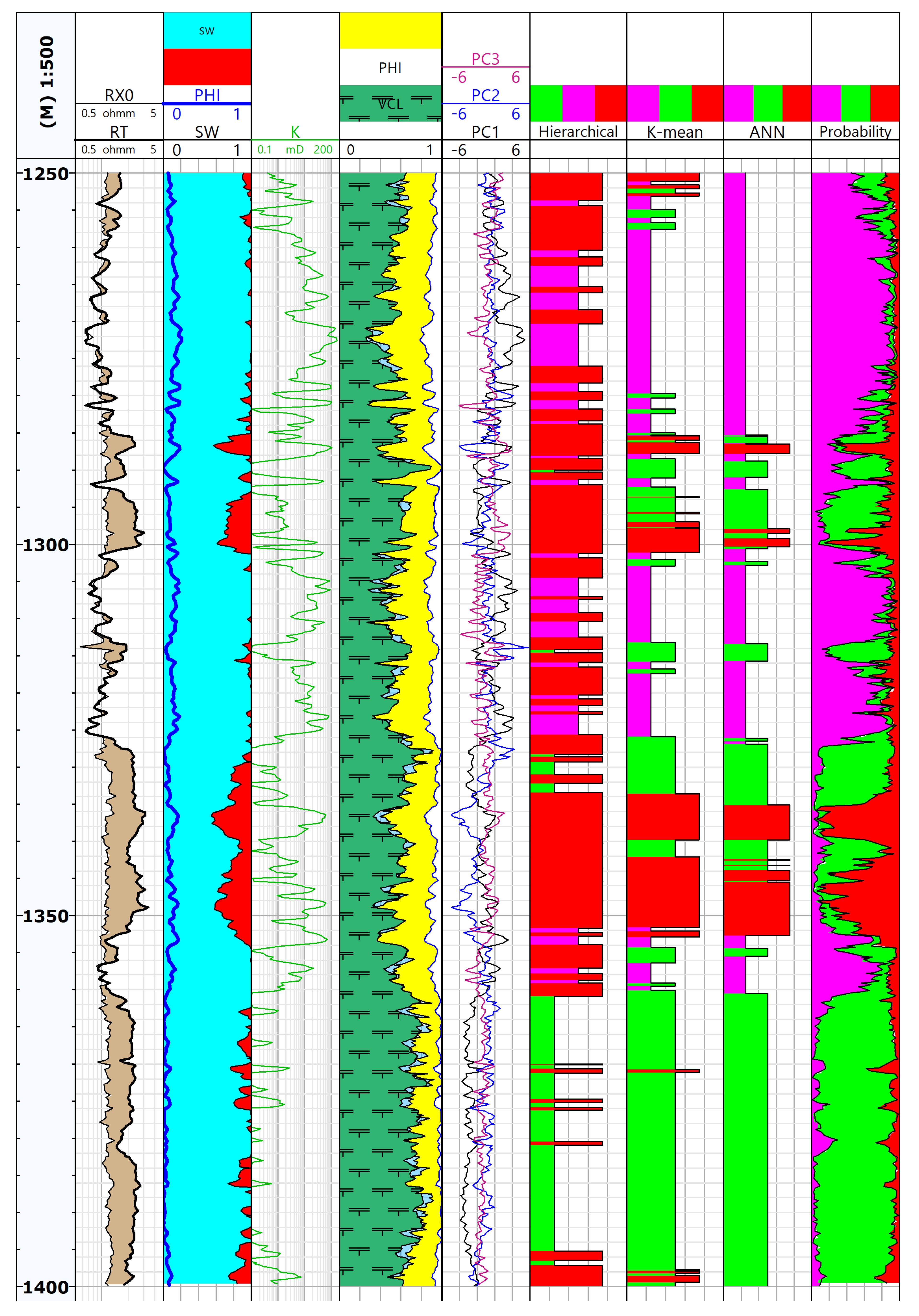
Figure 4 and Figure 5 depict the results of standard well log interpretation (these results were not taken into account during the calculations) and results of clustering. Tracks number 6–8 (Figure 4 for W-1 well and Figure 5 for W-2 well) contains the data division into three designated groups based on applied methods. The violet colour refers to group A, green to group B and red to group C.
W-1 well: Analysing the tested interval (Figure 4), can be noticed the agreement between the results of the comprehensive interpretation and the designated group A. The designated group A is a reflection of the layers with the highest water saturation, high permeability and represents the sandy-shaly formation. Group B represented by low porosity, low permeability and high water saturated claystone–sandstone formations, is also consistent with the results of a comprehensive interpretation. On the track 4—lithological track, the highest shale indications (green colour) correspond to group B, marked in green. Group C, determined during cluster analysis characterized by low water saturation and low porosity values correlates well with the results of comprehensive interpretation. The layers represented by group C may indicate hydrocarbon saturation. There is a strong correlation between the red layers (C cluster) and the lowest water saturation values on track number 2 (Figure 4).
Comparing groups distribution on the tracks 6 (Hierarchical cluster analysis results, HA), 7 (k-mean clustering results) and 8 (neural network algorithm results, ANN) there is a similarity between the ANN and k-mean results. The divisions have similar thicknesses and have been identified at similar depths. The greatest differences were observed in the depth interval: 1250–1270 m. Also, single, thin layers differ in the results obtained for these methods. The results of HA in the interval 1250–1370 differ from the other two methods. However, it should be noticed that the HA method classified some of the samples differently and assigned them to group 3 (gas saturated group). Comparison of the results of this method with hydrocarbon saturation (track number 2, red colour) indicates that k-mean and ANN included only significant volumes of hydrocarbons into group 3, while HA also captured low gas saturations.
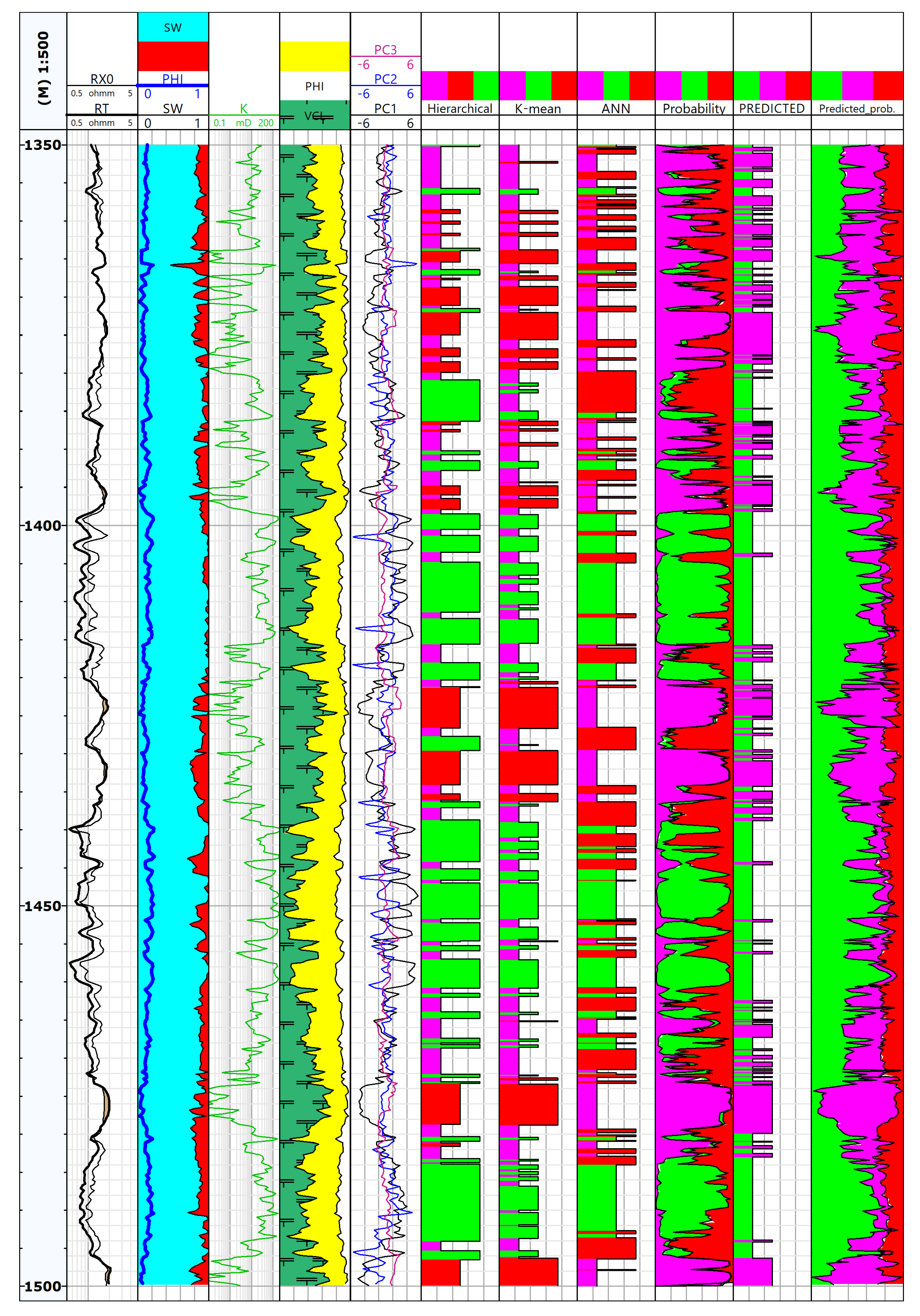
W-2 well: The occurrence of group A is adapted to the depth of the layers with the highest water saturation, high permeability and thin layers with a predominance of sandstone material over clay. The lowest permeability values correspond to group B, which are claystone-sandstone formations with poor reservoir parameters, however prospective in terms of the presence of gas, due to the relatively low water saturation. Group C, marked by layers of red colour, coincides with intervals of high permeability. In thin red layers, covering group C, can be additionally noticed the advantage of sandstone material over clay. Lowest indications of saturation with SW, presented on track 2, are correlated mainly in group C (red layers). In addition to low water saturation, group B also has low permeability values, which does not allow class B to be classified as well with good reservoir performance. Red layers from group C are correlated with increased permeability values (track number 3), which together with low water saturation indicates good reservoir parameters group C and the possibility of hydrocarbons (Figure 5).
Comparing the results obtained from the three methods of classification, in the W-2 well a much greater similarity than in the W-1 well. All these methods gave comparable results, both in terms of the thickness of the intervals and the depth. It should be noticed that more thin layers were separated in W-2 well than in W-1 well. This is consistent with the lithologic description and characteristics of thin-layered Miocene deposits. In W-2 well, the results of a comprehensive interpretation show that there are no visible levels with hydrocarbon saturation (track 2, Figure 5). However, there are slight gas saturations practically throughout the entire interval.
Prediction results: In the second stage of the analysis, predictions of facial distribution were made. The results are shown in Figure 5 (track 10–11). The Kohonen network learned and trained on data from W-1 well was applied to predict the facies distribution in the second well (W-2).
As a result, a division into facets was obtained:
- facies A–at the depths corresponding to facies A and C from previous analyses (CA and ANN separately for wells W-1 and W-2);
- facies B–at the depths corresponding to group B from previous analyses.
Track 11 shows the probability of choosing the winning facies. It can be noticed that practically in the whole interval, the smallest probability of choosing C (red) can be observed, but it corresponds to the gas saturation distribution (track 2, Figure 5). This confirms the C facies as a facies identifying the depths with the best reservoir properties, saturated with hydrocarbons. Everywhere, where previous methods indicated the belonging to group C, the facies A was chosen (sandy–shaly, with low or medium reservoir properties) during prediction.
4. Discussion
Comparing the results of statistical analyses presented in Figure 4 and Figure 5, common relationships can be observed. In both cases, the characteristic feature is the presence of thin layers, which are often characterized by low water saturation, increased porosity and permeability. In terms of lithology, designated groups confirm the existence of sandstone and claystone formations. A characteristic feature in the profile obtained based on statistical analyses is the presence of thin layers intersecting layers of much greater thickness (especially in W-2 well), e.g., section consisting mainly of claystone and sandstone formations with poor reservoir parameters (Group B) is divided with thin layers of sandstone and claystone with good reservoir parameters (Group C). Thin layers, crossing the greater thickness, are characteristic of Miocene formations in the Carpathian Foredeep. The highest probability of occurrence of hydrocarbons exists in thin-layered intervals in facies C.
Neural network models provide better prediction results using training patterns obtained from learning in comparison to the conventional linear methods. Using neural networks allows better exploring the hidden information within the multidimensional data set. Neural network analysis, as one of the non-parametric methods is not based on restrictive assumptions about the probability distributions of input variables. Although in neural network methods it is not necessary to investigate the correlation and distribution of input variables, a basic statistical study of the input variables is a desirable step. Appropriate selection of input variables will increase the predictive accuracy of the network. The normalization of the training variables is one of the main steps. However, the selection of appropriate network parameters is subjectiveThe consistent use of geological background and interpretation of sedimentation are crucial for the successful neural network lithofacies prediction, in which descriptive information is intensively used in an empirical sense.
The number of logs and the choice of well logs input affect the accuracy of facies prediction results. Different facies have different sensitivity to the input logs. In well, when using e.g., PE, the accuracy is high. However, the additional input of NPHI does not greatly improve the accuracy. The reason for this is that different logs add different levels of ‘new’ information to the neural network. New independent information will significantly increase the identification ability, while unnecessary information may reduce the neural network recognition ability.
Petrophysical data was processed using unsupervised ANN methods. Unsupervised methods determine their clusters based on the initial data set. However, these methods tend to seclude characteristic patterns and to obtain classifications or new variables that can be interpreted with a physical meaning. An example of this type of methodologies is cluster analysis. Facies are determined by the physical properties of rocks to which the well logs are sensitive. Facies are based on characteristics taken from continuous measurements at scales of meters and even centimetres, whereas geological facies are based primarily on observational features taken at scales down to millimetres [34].
5. Conclusions
Neural network analysis coupled with CA, PCA and DA were applied to construct improved finer-scale facies models, and provide a better understanding of the lithology distribution in the Miocene-age shale formations in the Carpathian Foredeep in Poland.
Three facies in each well were created. Correlations and relationships of well logs and facies were explored with basic 1D, 2D, and multidimensional statistical data analyses.
Neural network parameters were determined for neural network learning process in unsupervised approach, and then used to predict facies on the second well. The main idea of the present comparison was to accurately predict electrofacies which has a very significant impact on other reservoir parameter calculations, such as lithology and depositional facies.
The main highlights are as follows:
- The ANN method has been successful for making a quantitative and qualitative correlation between predicted facies and reservoir parameters.
- Neural network models provide a robust method for predicting electrofacies from well logs in complex sandy-shaly reservoirs.
- Data examination, pre-processing, statistical analyses, and geological constraints are the most important factors to neural network modelling. The correct execution of these steps allows for the correct prediction of facies in new wells.
- Using neural network modelling, a combination of standard well logs interpretation and a modern approach to supporting reservoir modelling was achieved.
- ANN model speeds up evaluation of a reservoir. It increased the accuracy of investigation to minor thicknesses and to divide a formation into facies with characteristic petrophysical parameters.
- Statistical methods are a useful complement to comprehensive geophysical interpretation. In both wells, located in the area of the Carpathian Foredeep, thin-layered sandstone-claystone formations were found, gas saturated depth intervals were identified.
Acknowledgments
The authors thank the Dean of Faculty of Geology, Geophysics and Environmental Protection, AGH-UST for financial support (the research subsidy no. 16.16.140.315). AGH – UST software grants for Techlog (Schlumberger) and Statistica (Statsoft).
Conflicts of Interest
The authors declare no conflict of interest.
References
- Dorfman, M.H. New techniques in lithofacies determination and permeability prediction in carbonates using well logs. In Geological Applications of Wireline Logs; Hurst, A., Lovell, M.A., Morton, A.C., Eds.; Geological Society: London, UK, 1990; Volume 48, pp. 113–120. [Google Scholar]
- Serra, O.; Abbott, H.T. The Contribution of Logging Data to Sedimentology and Stratigraphy. Soc. Pet. Eng. J. 1982, 22, 117–131. [Google Scholar] [CrossRef]
- Lianshuang, Q.; Carr, T.R. Neural Network Prediction of Carbonate Lithofacies from Well Logs, Big Bow and Sand Arroyo Creek Fields, Southwest Kansas. Comput. Geosci. 2006, 32, 947–964. [Google Scholar]
- Dubois, M.K.; Bohling, G.G.C.; Chakrabarti, S. Comparison of Four Approaches to a Rock Facies Classification Problem. Comput. Geosci. 2007, 33, 599–617. [Google Scholar] [CrossRef]
- Saggaf, M.M.; Nebrija, E.L. A Fuzzy Logic Approach for the Estimation of Facies from Wireline Logs. Am. Assoc. Pet. Geol. Bull. 2003, 87, 1223–1240. [Google Scholar]
- He, J.; La Croix, A.D.; Wand, J.; Ding, W.; Underschultz, J.R. Using Neural Networks and the Markov Chain Approach for Facies Analysis and Prediction from Well Logs in the Precipice Sandstone and Evergreen Formation, Surat Basin, Australia. Mar. Pet. Geol. 2019, 101, 410–427. [Google Scholar] [CrossRef]
- Haykin, S. Neural Network: A Comprehansive Foundation; Prentice Hall: Upper Saddle River, NJ, USA, 1998. [Google Scholar]
- Horrocks, T.; Holden, E.J.; Wedge, D. Evaluation of automated lithology classification architectures using highly-sampled wireline logs for coal exploration. Comput. Geosci. 2015, 83, 209–218. [Google Scholar] [CrossRef]
- Yang, H.; Pan, H.; Ma, H.; Konaté, A.A.; Yao, J.; Guo, B. Performance of the synergetic wavelet transform and modified k-means clustering in lithology classification using nuclear log. J. Pet. Sci. Eng. 2016, 144, 1–9. [Google Scholar] [CrossRef]
- Borsaru, M.; Zhou, B.; Aizawa, T.; Karashima, H.; Hashimoto, T. Automated lithology prediction from pgnaa and other geophysical logs. Appl. Radiat. Isot. 2006, 64, 272–282. [Google Scholar] [CrossRef]
- Xie, Y.; Zhu, C.; Zhou, W.; Li, Z.; Tu, M. Evaluation of machine learning methods for formation lithology identification: A comparison of tuning processes and model performances. J. Pet. Sci. Eng. 2018, 139, 182–193. [Google Scholar] [CrossRef]
- Szabó, N.P. Shale volume estimation based on the factor analysis of well logging data. Acta Geophys. 2011, 59, 935–953. [Google Scholar] [CrossRef]
- Puskarczyk, E.; Jarzyna, J.; Porębski, S.J. Application of multivariate statistical methods for characterizing heterolithic reservoirs based on wireline logs—Example from the Carpathian Foredeep Basin (Middle Miocene, SE Poland). Geol. Q. 2015, 59, 157–168. [Google Scholar]
- Puskarczyk, E.; Jarzyna, J.; Wawrzyniak-Guz, K.; Krakowska, P.; Zych, M. Improved recognition of rock formation on the basis of well logging and laboratory experiments results using factor analysis. Acta Geophys. 2019, 67, 1809–1822. [Google Scholar] [CrossRef] [Green Version]
- Techlog. Available online: https://www.software.slb.com/products/techlog/techlog-petrophysics (accessed on 25 January 2020).
- Statistica. Available online: https://www.statsoft.pl/Pelna-lista-programow-Statistica/ (accessed on 25 January 2020).
- Myśliwiec, M. Mioceńskie skały zbiornikowe zapadliska przedkarpackiego. Przegląd Geol. 2004, 52/7, 581–592. (In Polish) [Google Scholar]
- Karnkowski, P. Miocene deposits of the Carpathian Foredeep (according to results of oil and gas prospecting). Geol. Q. 1994, 38, 377–394. [Google Scholar]
- Moss, B.; Seheult, A. Does principal component analysis have a role in the interpretation of petrophysical data? In Proceedings of the 28th Annual Logging Symposium Transactions, Society Professional Well Log Analysts, London, UK, 29 June–2 July 1987. [Google Scholar]
- Kaiser, H.F. The varimax criterion for analytic rotation in factor analysis. Psychometrika 1958, 23, 187–200. [Google Scholar] [CrossRef]
- Puskarczyk, E. Artificial neural networks as a tool for pattern recognition and electrofacies analysis in Polish Palaeozoic shale gas formations. Acta Geophys. 2019, 67, 1991–2003. [Google Scholar] [CrossRef] [Green Version]
- Szabó, N.P.; Dobroka, M.; Kavanda, R. Cluster analysis assisted float-encoded genetic algorithm for a more automated characterization of hydro-carbon reservoirs. Intell. Control Autom. 2013, 4, 362–370. [Google Scholar] [CrossRef] [Green Version]
- Sfidari, E.; Amina, A.; Kadkhodaie-Ilkhchi, A.; Chehrazi, A.; Zamanzadeh, S.M. Depositional Facies, Diagenetic Overprints and Sequence Stratigraphy of the Upper Surmeh Reservoir (Arab Formation) of Offshore Iran. J. Afr. Earth Sci. 2019, 149, 55–71. [Google Scholar] [CrossRef]
- Hand, D.; Mannila, H.; Smyth, P. Eksploracja Danych; Wydawnictwa Naukowo-Techniczne: Warszawa, Poland, 2005. (In Polish) [Google Scholar]
- Ward, J. Hierarchical Grouping to Optimize an Objective Function. J. Am. Stat. Assoc. 1963, 58/30, 236–244. [Google Scholar] [CrossRef]
- Stanisz, A. Przystępny Kurs Statystyki z Zastosowaniem STATISTICA PL na Przykładach z Medycyny Tom 3. Analizy Wielowymiarowe; StatSoft Polska Sp. z o. o.: Kraków, Poland, 2007. (In Polish) [Google Scholar]
- Gatnar, E. Symboliczne Metody Klasyfikacji Danych; Wydawnictwo Naukowe PWN: Warszawa, Polska, 1998. (In Polish) [Google Scholar]
- Shen, C.; Asante-Okyere, S.; Ziggah, Y.Y.; Wang, L.; Zhu, X. Group Method of Data Handling (GMDH) Lithology Identification Based on Wavelet Analysis and Dimensionality Reduction as Well Log Data Pre-Processing Techniques. Energies 2019, 12, 1509. [Google Scholar] [CrossRef] [Green Version]
- Nkurlu, B.M.; Shen, C.; Asante-Okyere, S.; Mulashani, A.K.; Chungu, J.; Wang, L. Prediction of Permeability Using Group Method of Data. Energies 2020, 13, 551. [Google Scholar] [CrossRef] [Green Version]
- Asante-Okyere, S.; Shen, C.; Ziggah, Y.Y.; Rulegeya, M.M.; Zhu, X. Investigating the Predictive Performance of Gaussian Process Regression in Evaluating Reservoir Porosity and Permeability. Energies 2018, 11, 3261. [Google Scholar] [CrossRef] [Green Version]
- Bishop, C. Neural Network for Pattern Recognition; Clearendon Press: Oxford, UK, 1995. [Google Scholar]
- McCleland, T.L.; Rumelhart, D.E. Parallel Distributed Processing; MIT Press: Cambridge, MA, USA, 1986. [Google Scholar]
- Kohonen, T. Self-Organized Formation of Topologically Correct Feature Maps. Biol. Cybern. 1982, 43, 59–69. [Google Scholar] [CrossRef]
- Stinco, P. Core and Log Data Integration the Key for Determining Electrofacies. In Proceedings of the SPWLA 47th Annual Logging Symposium, Veracruz, Mexico, 4–7 June 2006. [Google Scholar]
Figure 1.
Hierarchical clustering results: (a) W-1 well; (b) W-2 well.

Figure 2.
Clustering results (different colours on the graphs) in the relation to the standard well logs interpretation, W-1 well: (a) row data relation RHOB vs. NPHI; (b) volume of quartz mineral content VSAN in the relation to the water saturation SW; (c) water saturation SW relation to the PC1; (d) water saturation in the relation of PC2.

Figure 3.
Clustering results (different colours on the graphs) in the relation to the standard well logs interpretation, W-2 well: (a) row data relation RHOB vs. NPHI; (b) volume of quartz mineral content VSAN in the relation to the water saturation SW; (c) bulk density RHOB in the relation to the PC1; (d) neutron porosity in the relation to the permeability.

Figure 4.
Results of measured log (1 track), standard comprehensive well log data interpretation (track 2–4) and statistical analysis (track 5–9), W-1 well. Colours for facies identification: A–violet, B–green, C–red.
Figure 4.
Results of measured log (1 track), standard comprehensive well log data interpretation (track 2–4) and statistical analysis (track 5–9), W-1 well. Colours for facies identification: A–violet, B–green, C–red.

Figure 5.
Results of measured log (1 track), standard comprehensive well log data interpretation (track 2–4), results of calculations (track 5–9) and results of prediction (track 10–11), W-2 well. Colours for facies identification: A–violet, B–green, C–red.
Figure 5.
Results of measured log (1 track), standard comprehensive well log data interpretation (track 2–4), results of calculations (track 5–9) and results of prediction (track 10–11), W-2 well. Colours for facies identification: A–violet, B–green, C–red.


Table 1.
Eigenvalues and percentage of variance, W-1 and W-2 wells.
| W-1 | W-2 | |||||||
|---|---|---|---|---|---|---|---|---|
| PC | Eigenvalue | % of Total Variance | Cumulative Eigenvalue | Cumulative % of Variance | Eigenvalue | % of Total Variance | Cumulative Eigenvalue | Cumulative % of Variance |
| 1 | 4.14 | 46 | 4.14 | 46 | 5.55 | 62 | 5.55 | 62 |
| 2 | 1.87 | 21 | 6.00 | 67 | 1.75 | 19 | 7.30 | 81 |
| 3 | 1.24 | 14 | 7.24 | 80 | 0.79 | 9 | 8.09 | 90 |
| 4 | 0.61 | 7 | 7.85 | 87 | 0.31 | 3 | 8.40 | 93 |
| 5 | 0.34 | 4 | 8.19 | 91 | 0.25 | 3 | 8.65 | 96 |
| 6 | 0.31 | 3 | 8.50 | 94 | 0.19 | 2 | 8.83 | 98 |
| 7 | 0.25 | 3 | 8.75 | 97 | 0.09 | 1 | 8.92 | 99.1 |
| 8 | 0.13 | 1 | 8.88 | 99 | 0.04 | 0.5 | 8.96 | 99.6 |
| 9 | 0.12 | 1 | 9.00 | 100 | 0.04 | 0.4 | 9.00 | 100 |
Table 2.
Factor loadings for selected PCs, W-1 and W-2 wells.
| W-1 | W-2 | |||||
|---|---|---|---|---|---|---|
| PC1 | PC2 | PC3 | PC1 | PC2 | PC3 | |
| LLD | −0.74 | −0.47 | 0.29 | −0.90 | −0.20 | 0.03 |
| LLS | −0.74 | −0.42 | 0.16 | −0.85 | −0.34 | −0.16 |
| DT | 0.10 | −0.17 | 0.95 | −0.34 | 0.88 | 0.03 |
| NPHI | −0.19 | 0.81 | 0.14 | −0.52 | 0.79 | 0.10 |
| RHOB | −0.89 | 0.21 | −0.26 | −0.88 | −0.33 | −0.10 |
| PE | −0.87 | 0.20 | 0.03 | −0.95 | −0.11 | −0.11 |
| GR | −0.84 | 0.27 | 0.08 | −0.96 | 0.15 | −0.09 |
| GRKT | −0.84 | −0.26 | −0.21 | −0.88 | 0.13 | −0.11 |
| CALI | −0.17 | 0.75 | 0.30 | −0.50 | −0.20 | 0.84 |
| % of total variance | 46 | 21 | 14 | 62 | 19 | 9 |
| cumulative % of variance | 80 | 90 | ||||
Table 3.
Classification matrix, based on the discriminant function, W-1 and W-2 wells.
| W-1 | W-2 | |||||||
|---|---|---|---|---|---|---|---|---|
| Training N = 451 % Correct | A p = 0.32 | B p = 0.42 | C p = 0.26 | Training N = 438 % Correct | A p = 0.13 | B p = 0.50 | C p = 0.37 | |
| A | 100.00 | 144 | 0 | 0 | 86.2 | 50 | 5 | 3 |
| B | 99.47 | 1 | 189 | 0 | 100.0 | 0 | 219 | 0 |
| C | 88.03 | 1 | 13 | 103 | 95.7 | 0 | 7 | 154 |
| All | 96.67 | 146 | 202 | 103 | 96.6 | 50 | 231 | 157 |
| Test N = 150 % Correct | A p = 0.38 | B p = 0.35 | C p = 0.27 | Test N = 163 % Correct | A p = 0.13 | B p = 0.53 | C p = 0.34 | |
| A | 100.00 | 57 | 0 | 0 | 81.82 | 18 | 2 | 2 |
| B | 98.08 | 1 | 51 | 0 | 100.00 | 0 | 86 | 0 |
| C | 95.12 | 0 | 2 | 39 | 90.91 | 0 | 5 | 50 |
| All | 98.00 | 58 | 53 | 39 | 94.48 | 18 | 93 | 52 |
© 2020 by the author. Licensee MDPI, Basel, Switzerland. This article is an open access article distributed under the terms and conditions of the Creative Commons Attribution (CC BY) license (http://creativecommons.org/licenses/by/4.0/).
Share and Cite
MDPI and ACS Style
Puskarczyk, E. Application of Multivariate Statistical Methods and Artificial Neural Network for Facies Analysis from Well Logs Data: an Example of Miocene Deposits. Energies 2020, 13, 1548. https://doi.org/10.3390/en13071548
AMA Style
Puskarczyk E. Application of Multivariate Statistical Methods and Artificial Neural Network for Facies Analysis from Well Logs Data: an Example of Miocene Deposits. Energies. 2020; 13(7):1548. https://doi.org/10.3390/en13071548
Chicago/Turabian StylePuskarczyk, Edyta. 2020. "Application of Multivariate Statistical Methods and Artificial Neural Network for Facies Analysis from Well Logs Data: an Example of Miocene Deposits" Energies 13, no. 7: 1548. https://doi.org/10.3390/en13071548
Note that from the first issue of 2016, this journal uses article numbers instead of page numbers. See further details here.