Liquid Storage Characteristics of Nanoporous Particles in Shale: Rigorous Proof

Abstract

Different from conventional reservoirs, a significant proportion of oil is in an adsorbed or even immobile state in shale and tight rocks. There are established comprehensive mathematical models quantifying the adsorbed, immobile, and free oil contents in shale rocks. However, the conclusions of the monotonicity of the complicated models from sensitivity analysis might not be universal, and rigorous mathematical derivation is needed to demonstrate their rationale. In this paper, the models for oil/water storage in the nanoporous grains in shale, i.e., kerogen and clay, are achieved based on the aforementioned storage models. Rigorous analytical derivations are employed to strictly prove the monotonicity of the immobile and adsorbed models, which is the main purpose of this work. This work expands the applicability of the storage models, is fundamental and important for mobility analysis in shale reservoirs, and can shed light on its efficient exploration and development.

1. Introduction

The production of oil from conventional resources is declining, and unconventional reservoirs [1,2] have captured growing attention worldwide. Among those resources, shale reserves are inspiring and have huge potential to satisfy energy consumption. Nonetheless, the features of abundant nanoscale porosity [3] and poor pore connectivity [4,5,6] result in difficulties in its economic utilization. Different from conventional reservoirs, a significant proportion of oil is in an adsorbed or even immobile state in shale and tight rocks. Therefore, one of the most urgent and fundamental issues is the mobility [7] or occurrence state [8] in shale reservoirs. However, there has been limited research on this topic.

There are three states of shale oil states, namely free, adsorbed, and immobile. Wang et al. [9,10] adopted molecular simulation to explore oil adsorption characteristics of organic pores in shale in detail. Cui et al. [11] established the methodology to estimate the fractions of physically adsorbed, immobile, and free oil in shale rocks. This method is based on continuous pore size distribution and the Gaussian mixture model (as shown in

Table 1. Gaussian Mixture Model—literature review.

Year	Reference	Purpose
2017	Cui et al. [11]	Mathematical models quantifying the occurrence states of shale oil are established.
2015	Javadpour et al. [15]	Generation of organic and inorganic pore size distributions.
2015	Naraghi et al. [16]	Classification of pore-size distributions within organic and inorganic matter
2019	Feng et al. [17]	Same as above.
2019	Cui et al. [18]	Same as above.
2019	Xu et al. [19]	Same as above.

), and it considers different pore types (organic and inorganic) [12], different pore geometries (circular and slit) [13,14], and the multiscale attribute of pore size. The monotonicity of the models has been concluded, but it was through calculations instead of rigorous proof. The latter approach is needed to support the conclusions because the forms of the models are complicated, and, therefore, the conclusions based on limited calculations might not be universal.

Immobile and adsorbed oil mainly exist in organic nanopores (instead of inorganic pores). In consideration of the mathematical complexity of the models and the physical significance of immobile and adsorbed oil, it makes sense to focus on the nanoporous kerogen grains. Moreover, clay [20] is also rich in nanoporosity [21,22,23] and the regularities should be similar [24]. In addition, hydraulic fracturing is indispensable for the efficient development of shale reservoirs [25], and water can be trapped in clay [26,27,28] and kerogen [29,30,31,32,33]. In conclusion, the understanding of oil/water storage features in kerogen/clay is crucial.

In this paper, in the first half (Section 2.1 and Section 2.2), previous works on the Gaussian mixture model and subsequent storage models are described, and the applicability of the storage models is expanded (from oil storage in kerogen to oil/water storage in kerogen/clay). In the latter half (Section 2.3 and Section 2.4), rigorous proof of the monotonicity of storage models is provided. The latter half is the main purpose of this work. This work is fundamental and important for mobility analysis in shale reservoirs and can shed light on its efficient exploration and development.

2. Mathematical Models

2.1. Gaussian Mixture Model

It is assumed that the organic and inorganic pore size distributions conform to lognormal Gaussian distributions and are independent from each other. Based on this assumption, the total pore size distribution of shale containing organic matter can be expressed as [16]:

$$P(r)=\frac{P(F_{in})}{\sqrt{2\pi }{\sigma }_{in}}{e}^{-\frac{{(r-{\mu }_{in})}^2}{2{\sigma }_{in}^2}}+\frac{P(F_{or})}{\sqrt{2\pi }{\sigma }_{or}}{e}^{-\frac{{(r-{\mu }_{or})}^2}{2{\sigma }_{or}^2}}$$

(1)

where P(F) is the ratio of organic porosity to total porosity, µ and σ are the mean and standard deviation of pore radius distribution, and r is a random variable denoting pore radius. Subscripts or and in stand for organic and inorganic media, respectively. Among the aforementioned variables, µ, σ, and r are all log-transformed values. It should be noted that the nano-Gaussian component extracted from experimental pore size distribution includes not only organic pores, but also inorganic nanopores within clay [34,35]. The former works simply regarded this component as organic pores. For convenience, the subscript or is still used to represent all the pores corresponding to the nano-Gaussian component.

2.2. Storage Models

Based on Equation (1), Cui et al. [11] derived the following formulae for the fractions of adsorbed oil, M_ad; immobile oil, M_im; and free oil, M_fr within shale rocks:

$$\begin{array}{l}{M}_{ad}=\frac{P(F_{in})}{\sqrt{2\pi }{\sigma }_{in}}\cdot {\displaystyle \underset{{\log }_{10}{h}_{in}}{\overset{\infty }{\int }}{e}^{-\frac{{(r-{\mu }_{in})}^2}{2{\sigma }_{in}^2}}[\alpha \frac{2\cdot {10}^r{h}_{in}-h_{in}^2}{{10}^{2r}}+(1-\alpha )\frac{h_{in}}{{10}^r}]dr}\\ +\frac{P(F_{or})}{\sqrt{2\pi }{\sigma }_{or}}\cdot {\displaystyle \underset{{\log }_{10}{h}_{or}}{\overset{\infty }{\int }}{e}^{-\frac{{(r-{\mu }_{or})}^2}{2{\sigma }_{or}^2}}[\alpha \frac{2\cdot {10}^r{h}_{or}-h_{or}^2}{{10}^{2r}}+(1-\alpha )\frac{h_{or}}{{10}^r}]dr}\end{array}$$

(2)

$$M_{im}=P(F_{in}){\displaystyle \underset{-\infty }{\overset{{\log }_{10}{h}_{in}}{\int }}\frac{1}{\sqrt{2\pi }{\sigma }_{in}}{e}^{-\frac{{(r-{\mu }_{in})}^2}{2{\sigma }_{in}^2}}dr}+P(F_{or}){\displaystyle \underset{-\infty }{\overset{{\log }_{10}{h}_{or}}{\int }}\frac{1}{\sqrt{2\pi }{\sigma }_{or}}{e}^{-\frac{{(r-{\mu }_{or})}^2}{2{\sigma }_{or}^2}}dr}$$

(3)

$$M_{fr}=1-M_{im}-M_{ad}$$

(4)

where h is the thickness of the adsorption region and α is the volume ratio of circular pores. For both Equations (2) and (3), the first component represents the contribution of inorganic pores, while the second component accounts for the contribution of organic pores. Among all the variables used in the models [11]:

• The thickness of an adsorption region reflects the strength of solid-liquid interaction, influenced by the relevant proportion of light and heavy oil components [9], and the different definitions for the adsorption region as well;
• The porosity ratio indicates the richness (or Total Organic Carbon) and maturity of organic matter in shale rocks. As the maturity of organic matter grows, its porous structure becomes more developed, and organic porosity increases;
• The pore size variance implies the dispersion or complexity of the porous structure of shale;
• The volume ratio of circular pores quantifies the overall pore morphology in shale, and it is impacted by the geo-mechanical conditions, the mineralogy, etc.;
• The average pore radius is the most fundamental parameter characterizing the porous structure, and it reflects how tight the porous rock is.

There are several underlying assumptions [11] for the models:

• Only circular and slit pores are considered [13], and α is constant in spite of different pore sizes;
• The critical pore radius for immobile oil is equal to the thickness of the adsorption region. To be more exact, when pore radius is smaller than or equal to adsorption thickness, all oil stored in pores is immobile; when pore radius is larger than adsorption thickness, oil exists as adsorbed and free states.
• Water content is negligible, and only oil exists in the pores;
• The slight density difference (about 10%) between adsorbed and free oil is ignored;
• Immobile oil only refers to the oil trapped in the pore space resulting from van der Waals. If only the nanoporous Gaussian component is considered, Equations (2) and (3) can be simplified as:

$$M_{ad}=\frac{1}{\sqrt{2\pi }\sigma }\cdot {\displaystyle \underset{{\log }_{10}h}{\overset{\infty }{\int }}{e}^{-\frac{{(r-\mu )}^2}{2{\sigma }^2}}[\alpha \frac{2\cdot {10}^{r}h-h^2}{{10}^{2r}}+(1-\alpha )\frac{h}{{10}^r}]dr}$$

(5)

$$M_{im}=\frac{1}{\sqrt{2\pi }\sigma }{\displaystyle \underset{-\infty }{\overset{{\log }_{10}h}{\int }}{e}^{-\frac{{(r-\mu )}^2}{2{\sigma }^2}}dr}.$$

(6)

As mentioned in the introduction, water/oil storage characteristics in kerogen/clay are similar. Therefore, Equations (5) and (6) can generally represent water and oil storage in kerogen and clay particles, respectively. Rigorous proof of the monotonicity of the storage models follows.

2.3. Proof for the Adsorbed Model

In this subsection, the monotonicity of the adsorbed model is discussed in terms of volume ratio of circular pores (α), thickness of the adsorption region (h), and average pore radius (μ). It should be noted that the proof of variance of pore radius (σ) is too difficult and not achieved, as it is technically quite tricky to isolate it away from the integration term.

2.3.1. Volume Ratio of Circular Pores (α)

α is in the integration term of Equation (5), and it would be more convenient for analysis if it could be moved out of the integration term. Equation (5) can be transformed into:

$$M_{ad}=\frac{1}{\sqrt{2\pi }\sigma }\cdot [\alpha {\displaystyle \underset{{\log }_{10}h}{\overset{\infty }{\int }}{e}^{-\frac{{(r-\mu )}^2}{2{\sigma }^2}}h\frac{{10}^r-h}{{10}^{2r}}dr}+{\displaystyle \underset{{\log }_{10}h}{\overset{\infty }{\int }}{e}^{-\frac{{(r-\mu )}^2}{2{\sigma }^2}}\frac{h}{{10}^r}dr}].$$

(7)

The monotonicity of Equation (7) cannot be easily determined. Therefore, the partial differentiation of Equation (7) can be taken for α:

$$\frac{\partial M_{ad}}{\partial \alpha }=\frac{1}{\sqrt{2\pi }\sigma }{\displaystyle \underset{{\log }_{10}h}{\overset{\infty }{\int }}{e}^{-\frac{{(r-\mu )}^2}{2{\sigma }^2}}h\frac{{10}^r-h}{{10}^{2r}}dr}.$$

(8)

In the integration, r > log₁₀h, thus 10^r > h. As a result, δM_ad/δα > 0 always holds. Namely, a larger proportion of circular pores is usually indicative of larger storage capacity of adsorbed liquid.

2.3.2. Thickness of Adsorption Region (h)

Similarly, effort is made to move h out of the integration term first for convenience. Equation (5) can be transformed into:

$$\begin{array}{ll}{M}_{ad}& =\frac{1}{\sqrt{2\pi }\sigma }\cdot {\displaystyle \underset{{\log }_{10}h}{\overset{\infty }{\int }}{e}^{-\frac{{(r-\mu )}^2}{2{\sigma }^2}}[\alpha \frac{2\cdot {10}^{r}h-h^2}{{10}^{2r}}+(1-\alpha )\frac{h}{{10}^r}]dr}\\ & =\frac{1}{\sqrt{2\pi }\sigma }\cdot {\displaystyle \underset{{\log }_{10}h}{\overset{\infty }{\int }}{e}^{-\frac{{(r-\mu )}^2}{2{\sigma }^2}}[(1+\alpha )\frac{h}{{10}^r}-\alpha \frac{h^2}{{10}^{2r}}]dr}\\ & =\frac{1}{\sqrt{2\pi }\sigma }\cdot [h{\displaystyle \underset{{\log }_{10}h}{\overset{\infty }{\int }}{e}^{-\frac{{(r-\mu )}^2}{2{\sigma }^2}}\frac{1+\alpha }{{10}^r}dr}-h^2{\displaystyle \underset{{\log }_{10}h}{\overset{\infty }{\int }}{e}^{-\frac{{(r-\mu )}^2}{2{\sigma }^2}}\frac{\alpha }{{10}^{2r}}dr}]\end{array}$$

(9)

The monotonicity of Equation (9) cannot be easily determined. Therefore, the partial differentiation of Equation (9) is taken:

$$\begin{array}{ll}\frac{\partial M_{ad}}{\partial h}& =\frac{1}{\sqrt{2\pi }\sigma }\cdot [\underset{{log}_{10}h}{\overset{\infty }{\int }}{e}^{-\frac{{(r-\mu )}^2}{2{\sigma }^2}}\frac{1+\alpha }{{10}^r}dr-h{e}^{-\frac{{({log}_{10}h-\mu )}^2}{2{\sigma }^2}}\frac{1+\alpha }{h}\frac{1}{hln10}\\ & -2h\underset{{log}_{10}h}{\overset{\infty }{\int }}{e}^{-\frac{{(r-\mu )}^2}{2{\sigma }^2}}\frac{\alpha }{{10}^{2r}}dr+h^2{e}^{-\frac{{({log}_{10}h-\mu )}^2}{2{\sigma }^2}}\frac{\alpha }{h^2}\frac{1}{hln10}]\\ & =\frac{1}{\sqrt{2\pi }\sigma }\cdot [\underset{{log}_{10}h}{\overset{\infty }{\int }}{e}^{-\frac{{(r-\mu )}^2}{2{\sigma }^2}}\frac{1+\alpha }{{10}^r}dr-2h\alpha \underset{{log}_{10}h}{\overset{\infty }{\int }}{e}^{-\frac{{(r-\mu )}^2}{2{\sigma }^2}}\frac{1}{{10}^{2r}}dr\\ & -e^{-\frac{{({log}_{10}h-\mu )}^2}{2{\sigma }^2}}\frac{1}{hln10}]\end{array}$$

(10)

Again, the monotonicity or sign of Equation (10) cannot be easily determined. Therefore, the partial differentiation of Equation (10) is taken:

$$\begin{array}{ll}\frac{{\partial }^2{M}_{ad}}{\partial h^2}& =\frac{1}{\sqrt{2\pi }\sigma }\cdot \{-\frac{1}{hln10}{e}^{-\frac{{({log}_{10}h-\mu )}^2}{2{\sigma }^2}}\frac{1+\alpha }{h}-[2\alpha \underset{{log}_{10}h}{\overset{\infty }{\int }}{e}^{-\frac{{(r-\mu )}^2}{2{\sigma }^2}}\frac{1}{{10}^{2r}}dr\\ & -2h\alpha \frac{1}{hln10}{e}^{-\frac{{({log}_{10}h-\mu )}^2}{2{\sigma }^2}}\frac{1}{h^2}]+\frac{{log}_{10}h-\mu }{{\sigma }^2}\frac{1}{hln10}{e}^{-\frac{{({log}_{10}h-\mu )}^2}{2{\sigma }^2}}\frac{1}{hln10}\\ & +e^{-\frac{{({log}_{10}h-\mu )}^2}{2{\sigma }^2}}\frac{1}{h^{2}ln10}\}\\ & =\frac{1}{\sqrt{2\pi }\sigma }\cdot \{-2\alpha \underset{{log}_{10}h}{\overset{\infty }{\int }}{e}^{-\frac{{(r-\mu )}^2}{2{\sigma }^2}}\frac{1}{{10}^{2r}}dr+e^{-\frac{{({log}_{10}h-\mu )}^2}{2{\sigma }^2}}\\ & [\frac{{log}_{10}h-\mu }{{\sigma }^2}\frac{1}{h^2{(ln10)}^2}+\frac{\alpha }{h^{2}ln10}]\}\end{array}$$

(11)

Again, the monotonicity or sign of Equation (11) cannot be easily determined. Therefore, the partial differentiation of Equation (11) is taken:

$$\begin{array}{ll}\frac{{\partial }^3{M}_{ad}}{\partial h^3}& =\frac{1}{\sqrt{2\pi }\sigma }\cdot \{2\alpha \frac{1}{hln10}{e}^{-\frac{{({log}_{10}h-\mu )}^2}{2{\sigma }^2}}\frac{1}{h^2}-\frac{{log}_{10}h-\mu }{{\sigma }^2}\frac{1}{hln10}{e}^{-\frac{{({log}_{10}h-\mu )}^2}{2{\sigma }^2}}\\ & [\frac{{log}_{10}h-\mu }{{\sigma }^2}\frac{1}{h^2{(ln10)}^2}+\frac{\alpha }{h^{2}ln10}]+e^{-\frac{{({log}_{10}h-\mu )}^2}{2{\sigma }^2}}[\frac{1}{{\sigma }^2}\frac{1}{hln10}\\ & \frac{1}{h^2{(ln10)}^2}-\frac{{log}_{10}h-\mu }{{\sigma }^2}\frac{2}{h^3{(ln10)}^2}-\frac{2\alpha }{h^{3}ln10}]\}\\ & =\frac{1}{\sqrt{2\pi }\sigma }\cdot e^{-\frac{{({log}_{10}h-\mu )}^2}{2{\sigma }^2}}\frac{1}{h^3{\sigma }^4{(ln10)}^3}\{-{({log}_{10}h-\mu )}^2\\ & -(\alpha +2){\sigma }^{2}ln10({log}_{10}h-\mu )+{\sigma }^2\}\end{array}$$

(12)

The zero-points of Equation (12) can be obtained by solving:

$$-{({\log }_{10}h-\mu )}^2-(\alpha +2){\sigma }^2\ln 10({\log }_{10}h-\mu )+{\sigma }^2=0.$$

(13)

However, the expression of Equation (13) is still difficult for analysis. We can denote:

$$t={\log }_{10}h-\mu .$$

(14)

Therefore, Equation (13) can be simplified as:

$$t^2+(\alpha +2){\sigma }^2\ln 10\cdot t-{\sigma }^2=0.$$

(15)

This equation has two zero-points:

$$t_{1,2}=\frac{-(\alpha +2){\sigma }^2\ln 10\pm \sqrt{{(\alpha +2)}^2{\sigma }^4{(\ln 10)}^2+4{\sigma }^2}}{2}.$$

(16)

Therefore, ∂³M_ad/∂h³ is negative when t < t₁ or t > t₂, and is positive when t₁ < t< t₂. Based on Equation (14), Equation (13) has two roots about h:

$$h_{1,2}={10}^{t_{1,2}+\mu }.$$

(17)

Consequently, ∂³M_ad/∂h³ is negative (∂²M_ad/∂h² decreases) when 0 < h < h₁ or h > h₂, and positive (∂²M_ad/∂h² increases) when h₁ < h < h₂. In addition:

$$\begin{array}{l}\underset{h\to 0}{\lim }\frac{{\partial }^2{M}_{ad}}{\partial h^2}=\underset{h\to 0}{\lim }\frac{1}{\sqrt{2\pi }\sigma }\cdot \{-2\alpha {\displaystyle \underset{{\log }_{10}h}{\overset{\infty }{\int }}{e}^{-\frac{{(r-\mu )}^2}{2{\sigma }^2}}\frac{1}{{10}^{2r}}dr}+e^{-\frac{{({\log }_{10}h-\mu )}^2}{2{\sigma }^2}}\\ [\frac{{\log }_{10}h-\mu }{{\sigma }^2}\frac{1}{h^2{(\ln 10)}^2}+\frac{\alpha }{h^2\ln 10}]\}\\ =-\frac{2\alpha }{\sqrt{2\pi }\sigma }{\displaystyle \underset{-\infty }{\overset{\infty }{\int }}{e}^{-\frac{{(r-\mu )}^2}{2{\sigma }^2}}\frac{1}{{10}^{2r}}dr}+\frac{1}{\sqrt{2\pi }{\sigma }^3{(\ln 10)}^2}\\ \underset{h\to 0}{\lim }{e}^{-\frac{{({\log }_{10}h-\mu )}^2}{2{\sigma }^2}}\frac{{\log }_{10}h-\mu +\alpha {\sigma }^2\ln 10}{h^2}\end{array}$$

(18)

The latter part of Equation (18) can be calculated:

$$\begin{array}{l}\underset{h\to 0}{\lim }{e}^{-\frac{{({\log }_{10}h-\mu )}^2}{2{\sigma }^2}}\frac{{\log }_{10}h-\mu +\alpha {\sigma }^2\ln 10}{h^2}=-\underset{t\to -\infty }{\lim }{e}^{-\frac{t^2}{2{\sigma }^2}}\frac{-t-\alpha {\sigma }^2\ln 10}{{10}^{2(t+\mu )}}\\ =-\underset{t\to -\infty }{\lim }{e}^{-\frac{t^2}{2{\sigma }^2}}\frac{e^{\ln (-t-\alpha {\sigma }^2\ln 10)}}{e^{2(t+\mu )\ln 10}}=-\underset{t\to -\infty }{\lim }{e}^{-\frac{t^2}{2{\sigma }^2}+\ln (-t-\alpha {\sigma }^2\ln 10)-2(t+\mu )\ln 10}=0\end{array}$$

(19)

Therefore, Equation (18) can be simplified as:

$$\underset{h\to 0}{\lim }\frac{{\partial }^2{M}_{ad}}{\partial h^2}=-\frac{2\alpha }{\sqrt{2\pi }\sigma }{\displaystyle \underset{-\infty }{\overset{\infty }{\int }}{e}^{-\frac{{(r-\mu )}^2}{2{\sigma }^2}}\frac{1}{{10}^{2r}}dr}\le 0.$$

(20)

Similarly, it can be proved that:

$$\begin{array}{l}\underset{h\to +\infty }{\lim }\frac{{\partial }^2{M}_{ad}}{\partial h^2}=\underset{h\to +\infty }{\lim }\frac{1}{\sqrt{2\pi }\sigma }\cdot \{-2\alpha \underset{{log}_{10}h}{\overset{\infty }{\int }}{e}^{-\frac{{(r-\mu )}^2}{2{\sigma }^2}}\frac{1}{{10}^{2r}}dr+e^{-\frac{{({log}_{10}h-\mu )}^2}{2{\sigma }^2}}\\ [\frac{{log}_{10}h-\mu }{{\sigma }^2}\frac{1}{h^2{(ln10)}^2}+\frac{\alpha }{h^{2}ln10}]\}\\ =\frac{1}{\sqrt{2\pi }{\sigma }^3{(ln10)}^2}\underset{h\to +\infty }{\lim }{e}^{-\frac{{({log}_{10}h-\mu )}^2}{2{\sigma }^2}}\frac{{log}_{10}h-\mu }{h^2}\\ =\frac{1}{\sqrt{2\pi }{\sigma }^3{(ln10)}^2}\underset{t\to +\infty }{\lim }{e}^{-\frac{t^2}{2{\sigma }^2}}\frac{t}{{10}^{2(t+\mu )}}\\ =\frac{1}{\sqrt{2\pi }{\sigma }^3{(ln10)}^2}\underset{t\to +\infty }{\lim }{e}^{-\frac{t^2}{2{\sigma }^2}}\frac{e^{lnt}}{e^{2(t+\mu )ln10}}\\ =\frac{1}{\sqrt{2\pi }{\sigma }^3{(ln10)}^2}\underset{t\to +\infty }{\lim }{e}^{-\frac{t^2}{2{\sigma }^2}+lnt-2(t+\mu )ln10}=0\end{array}$$

(21)

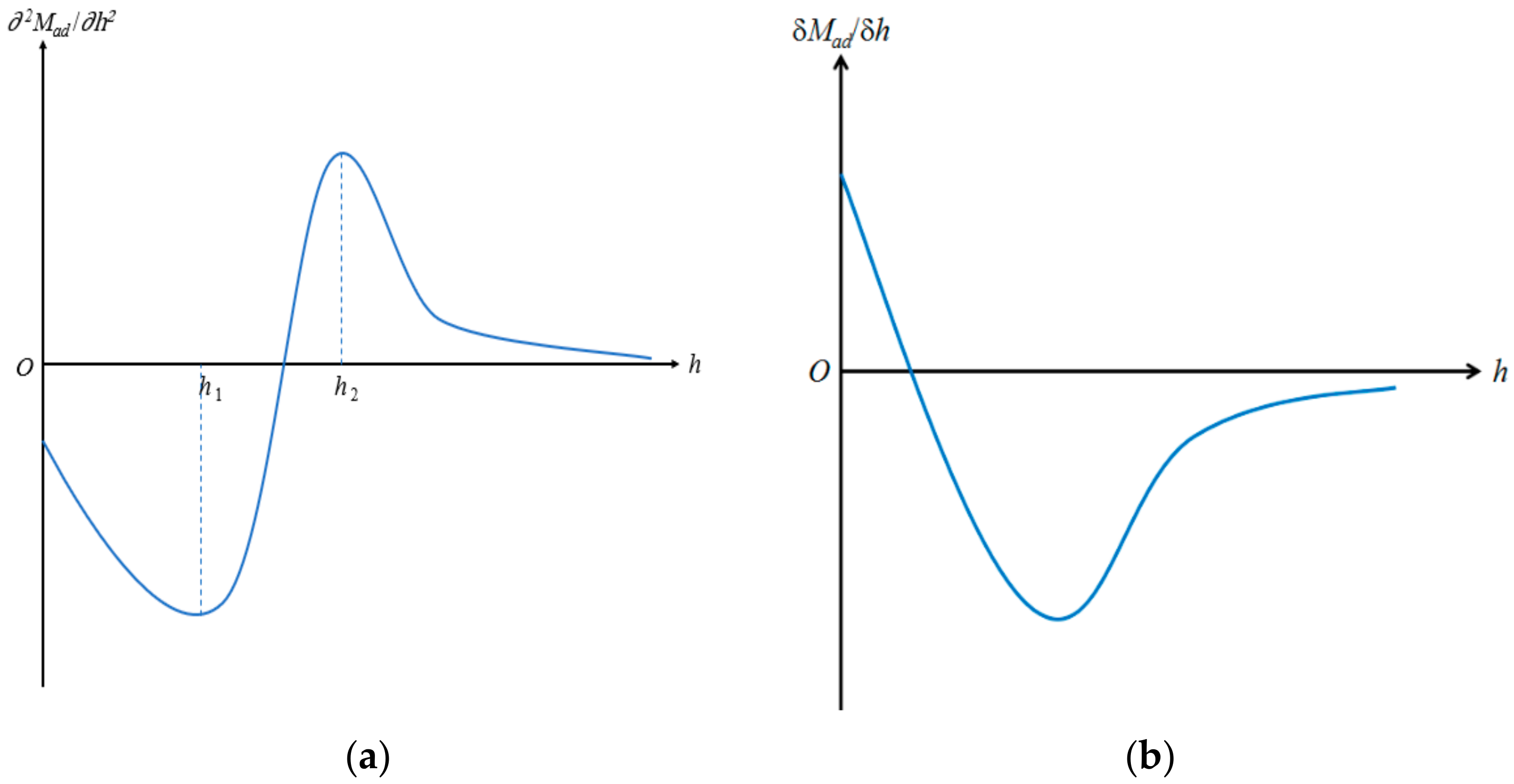
Based on the above conclusions (the limits of ∂²M_ad/∂h² at zero and infinity and the signs of ∂³M_ad/∂h³ at [0, h₁], [h₁, h₂], [h₂, +∞]), the graph of ∂²M_ad/∂h² can be sketched as Figure 1a. It can be determined that this derivative has and only has one zero-point h_a. ∂²M_ad/∂h² is negative (∂M_ad/∂h decreases) when h < h_a and positive (∂M_ad/∂h increases) when h > h_a.

In addition, it can be proved that:

$$\begin{array}{l}\underset{h\to +\infty }{lim}\frac{\partial M_{ad}}{\partial h}=\underset{h\to +\infty }{\lim }\frac{1}{\sqrt{2\pi }\sigma }\cdot [\underset{{log}_{10}h}{\overset{\infty }{\int }}{e}^{-\frac{{(r-\mu )}^2}{2{\sigma }^2}}\frac{1+\alpha }{{10}^r}dr\\ -2h\alpha \underset{{log}_{10}h}{\overset{\infty }{\int }}{e}^{-\frac{{(r-\mu )}^2}{2{\sigma }^2}}\frac{1}{{10}^{2r}}dr-e^{-\frac{{({log}_{10}h-\mu )}^2}{2{\sigma }^2}}\frac{1}{hln10}]\\ =-\frac{2\alpha }{\sqrt{2\pi }\sigma }\underset{h\to +\infty }{\lim }\frac{\underset{{log}_{10}h}{\overset{\infty }{\int }}{e}^{-\frac{{(r-\mu )}^2}{2{\sigma }^2}}\frac{1}{{10}^{2r}}dr}{h^{-1}}\\ =-\frac{2\alpha }{\sqrt{2\pi }\sigma }\underset{h\to +\infty }{\lim }\frac{e^{-\frac{{({log}_{10}h-\mu )}^2}{2{\sigma }^2}}\frac{1}{{10}^{2{log}_{10}h}}\frac{1}{hln10}}{h^{-2}}\\ =-\frac{2\alpha }{\sqrt{2\pi }\sigma }\underset{h\to +\infty }{\lim }{e}^{-\frac{{({log}_{10}h-\mu )}^2}{2{\sigma }^2}}\frac{1}{h^{5}ln10}=0\end{array}$$

(22)

Meanwhile, it can be proved that:

$$\begin{array}{l}\underset{h\to 0}{\lim }\frac{\partial M_{ad}}{\partial h}=\underset{h\to 0}{\lim }\frac{1}{\sqrt{2\pi }\sigma }\cdot [{\displaystyle \underset{{\log }_{10}h}{\overset{\infty }{\int }}{e}^{-\frac{{(r-\mu )}^2}{2{\sigma }^2}}\frac{1+\alpha }{{10}^r}dr}\\ -2h\alpha {\displaystyle \underset{{\log }_{10}h}{\overset{\infty }{\int }}{e}^{-\frac{{(r-\mu )}^2}{2{\sigma }^2}}\frac{1}{{10}^{2r}}dr}-e^{-\frac{{({\log }_{10}h-\mu )}^2}{2{\sigma }^2}}\frac{1}{h\ln 10}]\\ =\frac{1}{\sqrt{2\pi }\sigma }{\displaystyle \underset{-\infty }{\overset{\infty }{\int }}{e}^{-\frac{{(r-\mu )}^2}{2{\sigma }^2}}\frac{1+\alpha }{{10}^r}dr}-\frac{1}{\sqrt{2\pi }\sigma \ln 10}\underset{t\to -\infty }{\lim }{e}^{-\frac{t^2}{2{\sigma }^2}-(t+\mu )\ln 10}\\ =\frac{1}{\sqrt{2\pi }\sigma }{\displaystyle \underset{-\infty }{\overset{\infty }{\int }}{e}^{-\frac{{(r-\mu )}^2}{2{\sigma }^2}}\frac{1+\alpha }{{10}^r}dr}>0\end{array}$$

(23)

Based on the above conclusions (the limits of ∂M_ad/∂h at 0 and +∞, and the signs of ∂²M_ad/∂h² at [0, h_a], [h_a, +∞]), the graph of ∂M_ad/∂h can be sketched as Figure 1b. Therefore, ∂M_ad/∂h has and only has one zero-point, and consequently M_ad(h) first increases and then decreases with increasing adsorption thickness.

2.3.3. Average Pore Radius (μ)

Similarly, effort is made to move μ out of the integration term first for convenience. Equation (5) is rearranged in form at first, and then we can denote t = r-μ:

$$\begin{array}{ll}{M}_{ad}& =\frac{1}{\sqrt{2\pi }\sigma }\cdot [\underset{{log}_{10}h}{\overset{\infty }{\int }}{e}^{-\frac{{(r-\mu )}^2}{2{\sigma }^2}}[(1+\alpha )\frac{h}{{10}^r}-\alpha \frac{h^2}{{10}^{2r}}]dr\\ & =\frac{1}{\sqrt{2\pi }\sigma }\cdot [h(1+\alpha ){10}^{-\mu }\underset{{log}_{10}h}{\overset{\infty }{\int }}{e}^{-\frac{{(r-\mu )}^2}{2{\sigma }^2}}\frac{1}{{10}^{r-\mu }}dr\\ & -h^2\alpha {10}^{-2\mu }\underset{{log}_{10}h}{\overset{\infty }{\int }}{e}^{-\frac{{(r-\mu )}^2}{2{\sigma }^2}}\frac{1}{{10}^{2(r-\mu )}}dr\\ & =\frac{1}{\sqrt{2\pi }\sigma }\cdot [h(1+\alpha ){10}^{-\mu }\underset{{log}_{10}h-\mu }{\overset{\infty }{\int }}{e}^{-\frac{t^2}{2{\sigma }^2}}\frac{1}{{10}^t}dt\\ & -h^2\alpha {10}^{-2\mu }\underset{{log}_{10}h-\mu }{\overset{\infty }{\int }}{e}^{-\frac{t^2}{2{\sigma }^2}}\frac{1}{{10}^{2t}}dt]\end{array}$$

(24)

The monotonicity of Equation (24) cannot be easily determined. Therefore, the partial differentiation of Equation (24) is taken:

$$\begin{array}{c}\frac{\partial M_{ad}}{\partial \mu }=\frac{1}{\sqrt{2\pi }\sigma }\cdot [-\ln 10h(1+\alpha ){10}^{-\mu }{\displaystyle \underset{{\log }_{10}h-\mu }{\overset{\infty }{\int }}{e}^{-\frac{t^2}{2{\sigma }^2}}\frac{1}{{10}^t}dt}+(1+\alpha )e^{-\frac{{({\log }_{10}h-\mu )}^2}{2{\sigma }^2}}\\ +2\ln 10h^2\alpha {10}^{-2\mu }{\displaystyle \underset{{\log }_{10}h-\mu }{\overset{\infty }{\int }}{e}^{-\frac{t^2}{2{\sigma }^2}}\frac{1}{{10}^{2t}}dt}-\alpha e^{-\frac{{({\log }_{10}h-\mu )}^2}{2{\sigma }^2}}]\end{array}$$

(25)

Integral and non-integral terms coexist in Equation (25), and the integral term seems more difficult to deal with. Luckily, the non-integral term can be transformed and combined with the integral term:

$$\begin{array}{ll}\frac{\partial M_{ad}}{\partial \mu }& =\frac{1}{\sqrt{2\pi }\sigma }\cdot [-h(1+\alpha ){10}^{-\mu }ln10\underset{{log}_{10}h-\mu }{\overset{\infty }{\int }}{e}^{-\frac{t^2}{2{\sigma }^2}}\frac{1}{{10}^t}dt\\ & -(1+\alpha )h{10}^{-\mu }\underset{{log}_{10}h-\mu }{\overset{\infty }{\int }}d\left(e^{-\frac{t^2}{2{\sigma }^2}}\frac{1}{{10}^t}\right)+2h^2\alpha {10}^{-2\mu }ln10\\ & \underset{{log}_{10}h-\mu }{\overset{\infty }{\int }}{e}^{-\frac{t^2}{2{\sigma }^2}}\frac{1}{{10}^{2t}}dt+\alpha h^2{10}^{-2\mu }\underset{{log}_{10}h-\mu }{\overset{\infty }{\int }}d\left(e^{-\frac{t^2}{2{\sigma }^2}}\frac{1}{{10}^{2t}}\right)]\\ & =\frac{1}{\sqrt{2\pi }\sigma }\cdot [-h(1+\alpha ){10}^{-\mu }ln10\underset{{log}_{10}h-\mu }{\overset{\infty }{\int }}{e}^{-\frac{t^2}{2{\sigma }^2}}\frac{1}{{10}^t}dt+(1+\alpha )h{10}^{-\mu }\\ & \underset{{log}_{10}h-\mu }{\overset{\infty }{\int }}(ln10+\frac{t}{{\sigma }^2})e^{-\frac{t^2}{2{\sigma }^2}}\frac{1}{{10}^t}dt+2h^2\alpha {10}^{-2\mu }ln10\underset{{log}_{10}h-\mu }{\overset{\infty }{\int }}{e}^{-\frac{t^2}{2{\sigma }^2}}\frac{1}{{10}^{2t}}dt\\ & -\alpha h^2{10}^{-2\mu }\underset{{log}_{10}h-\mu }{\overset{\infty }{\int }}(2ln10+\frac{t}{{\sigma }^2})e^{-\frac{t^2}{2{\sigma }^2}}\frac{1}{{10}^{2t}}dt]\\ & =\frac{h{10}^{-\mu }}{\sqrt{2\pi }{\sigma }^3}\cdot [(1+\alpha )\underset{{log}_{10}h-\mu }{\overset{\infty }{\int }}{e}^{-\frac{t^2}{2{\sigma }^2}}\frac{t}{{10}^t}dt-\alpha h{10}^{-\mu }\underset{{log}_{10}h-\mu }{\overset{\infty }{\int }}{e}^{-\frac{t^2}{2{\sigma }^2}}\frac{t}{{10}^{2t}}dt]\end{array}$$

(26)

The signs of the integral terms in Equation (26) need further determination. A new function is introduced and defined as the expression in the brackets of Equation (26):

$$f(\mu )=(1+\alpha ){\displaystyle \underset{{\log }_{10}h-\mu }{\overset{\infty }{\int }}{e}^{-\frac{t^2}{2{\sigma }^2}}\frac{t}{{10}^t}dt}-\alpha h{10}^{-\mu }{\displaystyle \underset{{\log }_{10}h-\mu }{\overset{\infty }{\int }}{e}^{-\frac{t^2}{2{\sigma }^2}}\frac{t}{{10}^{2t}}dt}.$$

(27)

The monotonicity of Equation (27) cannot be easily determined. Therefore, the partial derivation of Equation (27) is taken:

$$\begin{array}{ll}{f}^{\prime }(\mu )& =(1+\alpha )h^{-1}{10}^{\mu }{e}^{-\frac{{({\log }_{10}h-\mu )}^2}{2{\sigma }^2}}({\log }_{10}h-\mu )\\ & +\alpha \ln 10\cdot h{10}^{-\mu }{\displaystyle \underset{{\log }_{10}h-\mu }{\overset{\infty }{\int }}{e}^{-\frac{t^2}{2{\sigma }^2}}\frac{t}{{10}^{2t}}dt}-\alpha h^{-1}{10}^{\mu }{e}^{-\frac{{({\log }_{10}h-\mu )}^2}{2{\sigma }^2}}({\log }_{10}h-\mu )\\ & =h^{-1}{10}^{\mu }{e}^{-\frac{{({\log }_{10}h-\mu )}^2}{2{\sigma }^2}}({\log }_{10}h-\mu )+\alpha \ln 10\cdot h{10}^{-\mu }{\displaystyle \underset{{\log }_{10}h-\mu }{\overset{\infty }{\int }}{e}^{-\frac{t^2}{2{\sigma }^2}}\frac{t}{{10}^{2t}}dt}\end{array}$$

(28)

Again, integral and non-integral terms coexist in Equation (28), and the integral term seems more difficult to deal with. Luckily, the non-integral term can be transformed and combined with the integral term:

$$\begin{array}{ll}{f}^{\prime }(\mu )& =-h^{-1}{10}^{\mu }[h^2{10}^{-2\mu }{\displaystyle \underset{{\log }_{10}h-\mu }{\overset{\infty }{\int }}d(e^{-\frac{t^2}{2{\sigma }^2}}\frac{t}{{10}^{2t}})}]\\ & +\alpha \ln 10\cdot h{10}^{-\mu }{\displaystyle \underset{{\log }_{10}h-\mu }{\overset{\infty }{\int }}{e}^{-\frac{t^2}{2{\sigma }^2}}\frac{t}{{10}^{2t}}dt}\\ & =h{10}^{-\mu }{\displaystyle \underset{{\log }_{10}h-\mu }{\overset{\infty }{\int }}{e}^{-\frac{t^2}{2{\sigma }^2}}{10}^{-2\mathrm{t}}(\frac{t^2}{{\sigma }^2}+2\ln 10\cdot t-1)dt}\\ & +\alpha \ln 10\cdot h{10}^{-\mu }{\displaystyle \underset{{\log }_{10}h-\mu }{\overset{\infty }{\int }}{e}^{-\frac{t^2}{2{\sigma }^2}}{10}^{-2\mathrm{t}}tdt}\\ & =h{10}^{-\mu }{\displaystyle \underset{{\log }_{10}h-\mu }{\overset{\infty }{\int }}{e}^{-\frac{t^2}{2{\sigma }^2}}{10}^{-2\mathrm{t}}[\frac{t^2}{{\sigma }^2}+(2+\alpha )\ln 10\cdot t-1]dt}\end{array}$$

(29)

However, the sign of the integral term in Equation (29) is still difficult to determine. Another new function is defined as the integration in Equation (29):

$$g(\mu )={\displaystyle \underset{{\log }_{10}h-\mu }{\overset{\infty }{\int }}{e}^{-\frac{t^2}{2{\sigma }^2}}{10}^{-2\mathrm{t}}[\frac{t^2}{{\sigma }^2}+(2+\alpha )\ln 10\cdot t-1]dt}.$$

(30)

The monotonicity of Equation (30) cannot be easily determined. Therefore, the partial differentiation of Equation (30) is taken:

$$g^{\prime }(\mu )=h^{-2}{10}^{2\mu }{e}^{-\frac{{({\log }_{10}h-\mu )}^2}{2{\sigma }^2}}[\frac{{({\log }_{10}h-\mu )}^2}{{\sigma }^2}+(2+\alpha )\ln 10\cdot ({\log }_{10}h-\mu )-1].$$

(31)

The zero-points of Equation (31) can be obtained by solving:

$$\frac{{({\log }_{10}h-\mu )}^2}{{\sigma }^2}+(2+\alpha )\ln 10\cdot ({\log }_{10}h-\mu )-1=0.$$

(32)

However, the expression of Equation (32) is still difficult to analyze. When we denote t = log₁₀h-μ, Equation (32) can be simplified as:

$$\frac{t^2}{{\sigma }^2}+(2+\alpha )\ln 10\cdot t-1=0.$$

(33)

This equation has two zero-points:

$$\begin{array}{l}{t}_{1,2}=\frac{-(2+\alpha )\ln 10\pm \sqrt{{(2+\alpha )}^2{(\ln 10)}^2+4/{\sigma }^2}}{2/{\sigma }^2}\\ =\frac{-(2+\alpha )\ln 10{\sigma }^2\pm \sqrt{{(2+\alpha )}^2{(\ln 10)}^2{\sigma }^4+4{\sigma }^2}}{2}\end{array}$$

(34)

Therefore, g’(μ) is positive when t < t₁ or t > t₂, and negative when t₁ < t < t₂. Equation (32) has two roots:

$${\mu }_{2,1}={\log }_{10}h-t_{1,2}.$$

(35)

Therefore, g’(μ) is positive (g(μ) increases) when 𝜇 < μ₁ or 𝜇 > μ₂, and negative (g(μ) decreases) when μ₁ < 𝜇 < μ₂. In addition:

$$\underset{\mu \to -\infty }{\lim }g(\mu )=\underset{\mu \to -\infty }{\lim }{\displaystyle \underset{{\log }_{10}h-\mu }{\overset{\infty }{\int }}{e}^{-\frac{t^2}{2{\sigma }^2}}{10}^{-2\mathrm{t}}[\frac{t^2}{{\sigma }^2}+(2+\alpha )\ln 10\cdot t-1]dt}=0.$$

(36)

Meanwhile:

$$\begin{array}{ll}\underset{\mu \to +\infty }{\lim }g(\mu )& =\underset{\mu \to +\infty }{\lim }{\displaystyle \underset{{\log }_{10}h-\mu }{\overset{\infty }{\int }}{e}^{-\frac{t^2}{2{\sigma }^2}}{10}^{-2\mathrm{t}}[\frac{t^2}{{\sigma }^2}+(2+\alpha )\ln 10\cdot t-1]dt}\\ & ={\displaystyle \underset{-\infty }{\overset{\infty }{\int }}{e}^{-\frac{t^2}{2{\sigma }^2}}{10}^{-2\mathrm{t}}[\frac{t^2}{{\sigma }^2}+(2+\alpha )\ln 10\cdot t-1]dt}\end{array}$$

(37)

It is difficult to determine the sign of Equation (37). It is regarded as a function of α:

$$w(\alpha )={\displaystyle \underset{-\infty }{\overset{\infty }{\int }}{e}^{-\frac{t^2}{2{\sigma }^2}}{10}^{-2\mathrm{t}}[\frac{t^2}{{\sigma }^2}+(2+\alpha )\ln 10\cdot t-1]dt}.$$

(38)

The partial derivation of Equation (38) is taken:

$$w^{\prime }(\alpha )=\frac{\partial }{\partial \alpha }{\displaystyle \underset{-\infty }{\overset{\infty }{\int }}{e}^{-\frac{t^2}{2{\sigma }^2}}{10}^{-2\mathrm{t}}[\frac{t^2}{{\sigma }^2}+(2+\alpha )\ln 10\cdot t-1]dt}=\ln 10{\displaystyle \underset{-\infty }{\overset{\infty }{\int }}{e}^{-\frac{t^2}{2{\sigma }^2}}{10}^{-2\mathrm{t}}tdt}.$$

(39)

It can be proved that Equation (39) is negative:

$$\begin{array}{l}{w}^{\prime }(\alpha )=\ln 10{\displaystyle \underset{-\infty }{\overset{\infty }{\int }}{e}^{-\frac{t^2}{2{\sigma }^2}}{10}^{-2\mathrm{t}}tdt}=\ln 10[{\displaystyle \underset{-\infty }{\overset{0}{\int }}{e}^{-\frac{t^2}{2{\sigma }^2}}{10}^{-2\mathrm{t}}tdt}+{\displaystyle \underset{0}{\overset{\infty }{\int }}{e}^{-\frac{t^2}{2{\sigma }^2}}{10}^{-2\mathrm{t}}tdt}]\\ =\ln 10[-{\displaystyle \underset{0}{\overset{+\infty }{\int }}{e}^{-\frac{t^2}{2{\sigma }^2}}{10}^{2\mathrm{t}}tdt}+{\displaystyle \underset{0}{\overset{\infty }{\int }}{e}^{-\frac{t^2}{2{\sigma }^2}}{10}^{-2\mathrm{t}}tdt}]\\ =\ln 10{\displaystyle \underset{0}{\overset{+\infty }{\int }}{e}^{-\frac{t^2}{2{\sigma }^2}}t({10}^{-2\mathrm{t}}-{10}^{2\mathrm{t}})dt}<0\end{array}$$

(40)

Therefore, w(α) decreases on (0, 1). Considering that:

$$\begin{array}{l}w(0)={\displaystyle \underset{-\infty }{\overset{\infty }{\int }}{e}^{-\frac{t^2}{2{\sigma }^2}}{10}^{-2\mathrm{t}}(\frac{t^2}{{\sigma }^2}+2\ln 10\cdot t-1)dt}=-{\displaystyle \underset{-\infty }{\overset{\infty }{\int }}d(e^{-\frac{t^2}{2{\sigma }^2}}\frac{t}{{10}^{2t}})}\\ =\underset{t\to +\infty }{\lim }{e}^{-\frac{t^2}{2{\sigma }^2}}\frac{t}{{10}^{2t}}-\underset{t\to -\infty }{\lim }{e}^{-\frac{t^2}{2{\sigma }^2}}\frac{t}{{10}^{2t}}\\ =\underset{t\to +\infty }{\lim }{e}^{-\frac{t^2}{2{\sigma }^2}+\ln t-2t\ln 10}+\underset{t\to -\infty }{\lim }{e}^{-\frac{t^2}{2{\sigma }^2}+\ln (-t)-2t\ln 10}=0\end{array}$$

(41)

Hence, w(α) is negative, which means that:

$$\underset{\mu \to +\infty }{\lim }g(\mu )={\displaystyle \underset{-\infty }{\overset{\infty }{\int }}{e}^{-\frac{t^2}{2{\sigma }^2}}{10}^{-2\mathrm{t}}[\frac{t^2}{{\sigma }^2}+(2+\alpha )\ln 10\cdot t-1]dt}<0.$$

(42)

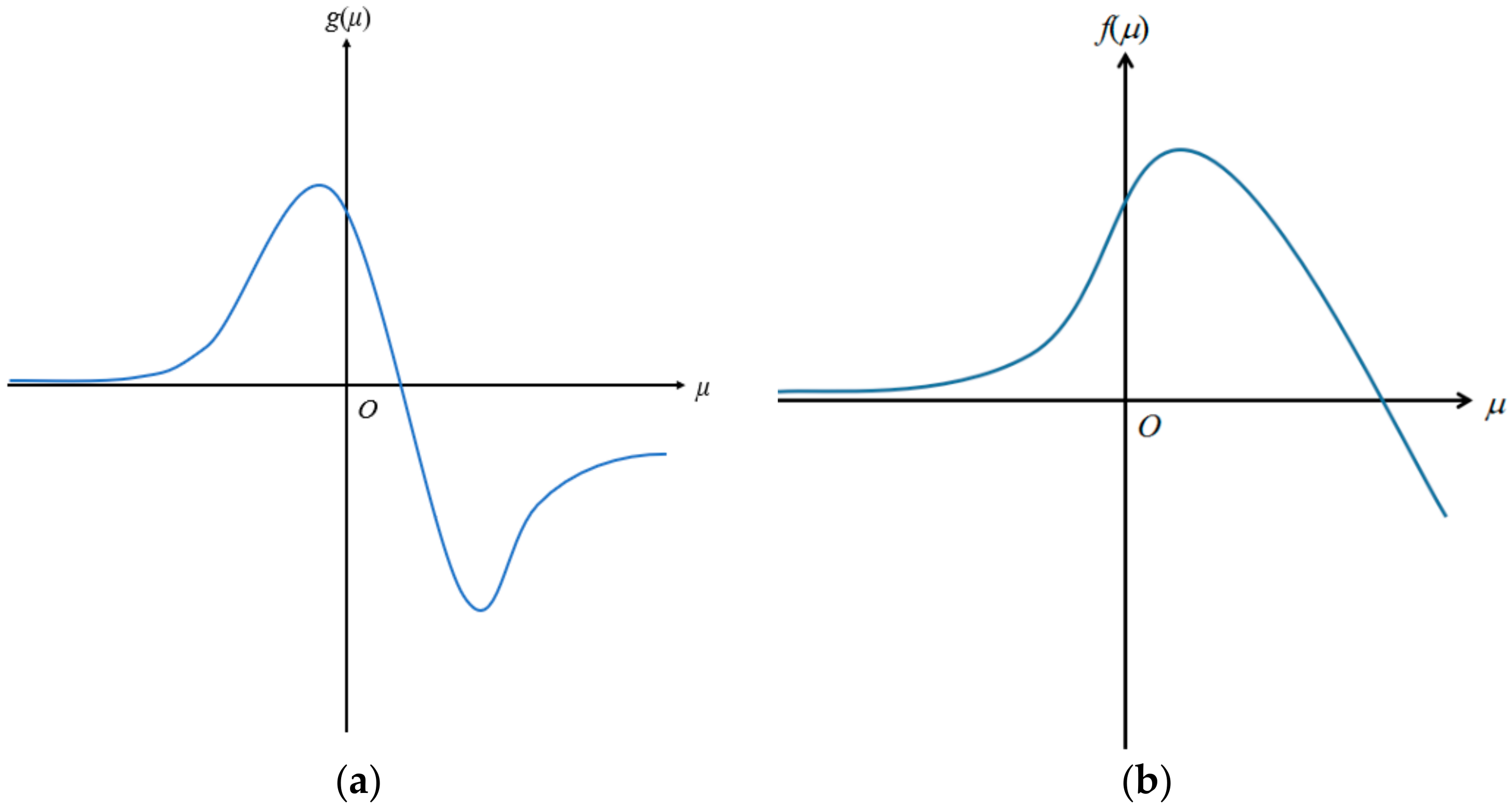
Based on the above conclusions (the limits of g(μ) at 0 and +∞, and the signs of g’(μ) at [-∞, μ₁], [μ₁, μ₂], [μ₂, +∞]), the graph of g(μ) can be sketched as Figure 2a. From this graph, it can be concluded that g(μ) has and only has one zero-point, μ_a. g(μ) > 0 when μ < μ_a, and g(μ) < 0 when μ > μ_a. Therefore, f ’(μ) only has one zero-point, μ_a. When μ < μ_a, f ’(μ) > 0 (f(μ) increases); When μ > μ_a, f ’(μ) < 0 (f(μ) decreases). In addition:

$$\begin{array}{l}\underset{\mu \to +\infty }{\lim }f(\mu )=(1+\alpha ){\displaystyle \underset{-\infty }{\overset{+\infty }{\int }}{e}^{-\frac{t^2}{2{\sigma }^2}}\frac{t}{{10}^t}dt}=(1+\alpha )[{\displaystyle \underset{-\infty }{\overset{0}{\int }}{e}^{-\frac{t^2}{2{\sigma }^2}}\frac{t}{{10}^t}dt}+{\displaystyle \underset{0}{\overset{+\infty }{\int }}{e}^{-\frac{t^2}{2{\sigma }^2}}\frac{t}{{10}^t}dt}]\\ =(1+\alpha )[-{\displaystyle \underset{0}{\overset{+\infty }{\int }}t{10}^t{e}^{-\frac{t^2}{2{\sigma }^2}}dt}+{\displaystyle \underset{0}{\overset{+\infty }{\int }}{e}^{-\frac{t^2}{2{\sigma }^2}}\frac{t}{{10}^t}dt}]\\ =(1+\alpha ){\displaystyle \underset{0}{\overset{+\infty }{\int }}t{e}^{-\frac{t^2}{2{\sigma }^2}}(\frac{1}{{10}^t}-{10}^t)dt}<0\end{array}$$

(43)

Meanwhile:

$$\underset{\mu \to -\infty }{\lim }f(\mu )=\underset{\mu \to -\infty }{\lim }\left[(1+\alpha ){\displaystyle \underset{{\log }_{10}h-\mu }{\overset{\infty }{\int }}{e}^{-\frac{t^2}{2{\sigma }^2}}\frac{t}{{10}^t}dt}-\alpha h{10}^{-\mu }{\displaystyle \underset{{\log }_{10}h-\mu }{\overset{\infty }{\int }}{e}^{-\frac{t^2}{2{\sigma }^2}}\frac{t}{{10}^{2t}}dt}\right].$$

(44)

For both terms of Equation (44), the integration terms approach zero as the lower limits approach infinity, which are the same as the upper limits. Therefore, the first term of Equation (44) approaches zero. However, for the second term of Equation (44), the expression before the integration term approaches infinity, therefore the limit of the second term of Equation (44) is uncertain and needs further determination:

$$\begin{array}{l}\underset{\mu \to -\infty }{\lim }f(\mu )=-\alpha \underset{\mu \to -\infty }{\lim }\frac{{\displaystyle \underset{{\log }_{10}h-\mu }{\overset{\infty }{\int }}{e}^{-\frac{t^2}{2{\sigma }^2}}\frac{t}{{10}^{2t}}dt}}{h^{-1}{10}^{\mu }}\\ =-\alpha \underset{\mu \to -\infty }{\lim }\frac{e^{-\frac{{({\log }_{10}h-\mu )}^2}{2{\sigma }^2}}{10}^{-2({\log }_{10}h-\mu )}({\log }_{10}h-\mu )}{h^{-1}{10}^{\mu }\ln 10}\\ =-\frac{\alpha }{\ln 10}\underset{t\to +\infty }{\lim }\frac{e^{-\frac{t^2}{2{\sigma }^2}}{10}^{-2t}t}{{10}^t}=-\frac{\alpha }{\ln 10}\underset{t\to +\infty }{\lim }{e}^{-\frac{t^2}{2{\sigma }^2}-3t\ln 10+\ln t}=0\end{array}$$

(45)

Based on the above conclusions (the limits of f(μ) at -∞ and +∞, and the signs of f’(μ) at [-∞, μ_a], [μ_a, +∞]), the graph of f(μ) can be sketched as Figure 2b. From this graph, f(μ) has and only has one zero-point. Therefore, M_ad(μ) first increases and then decreases with increasing average pore radius.

2.4. Proof for the Immobile Model

In this subsection, the monotonicity of the immobile model is analyzed in terms of thickness of the adsorption region (h), variance of pore radius (σ), average pore radius (μ), and volume ratio of circular pores (α). It is noteworthy that all the variables are analyzed here.

2.4.1. Thickness of Adsorption Region (h)

The monotonicity of Equation (6) cannot be easily determined. Therefore, the partial differentiation of Equation (6) is taken for h:

$$\frac{\partial M_{im}}{\partial h}=\frac{1}{\sqrt{2\pi }\sigma }{e}^{-\frac{{({\log }_{10}h-\mu )}^2}{2{\sigma }^2}}\frac{1}{h\ln 10}.$$

(46)

It is apparent that δM_im/δh is always positive, and M_im increases with the increase of h.

2.4.2. Variance of Pore Radius (σ)

σ is contained in the integration function of Equation (6), and the corresponding partial derivative cannot be directly taken. Instead, variable substitution is utilized for solving. If we denote t = (r-μ)/σ, then r = tσ+μ and Equation (6) is transformed into:

$$M_{im}=\frac{1}{\sqrt{2\pi }}{\displaystyle \underset{-\infty }{\overset{\frac{{\log }_{10}h-\mu }{\sigma }}{\int }}{e}^{-\frac{1}{2}{t}^2}dt}.$$

(47)

The monotonicity of Equation (47) cannot be easily determined. Therefore, the partial derivative of Equation (47) is taken for σ:

$$\frac{\partial M_{im}}{\partial \sigma }=\frac{1}{\sqrt{2\pi }}{e}^{-\frac{1}{2}{(\frac{{\log }_{10}h-\mu }{\sigma })}^2}\frac{\mu -{\log }_{10}h}{{\sigma }^2}.$$

(48)

If μ > log₁₀h, δM_im/δσ > 0. Otherwise, δM_im/δσ < 0. Hence, M_im will increase with increasing σ if μ > log₁₀h, and decrease with the increment of σ when μ < log₁₀h.

2.4.3. Average Pore Radius (μ)

The partial differentiation for μ is obtained in a similar way. If we denote t = r-μ, r = t+μ, and Equation (6) is transformed into:

$$M_{im}=\frac{1}{\sqrt{2\pi }\sigma }{\displaystyle \underset{-\infty }{\overset{{\log }_{10}h-\mu }{\int }}{e}^{-\frac{t^2}{2{\sigma }^2}}dt}.$$

(49)

Again, the monotonicity of Equation (49) cannot be easily determined. Therefore, the partial derivation of Equation (49) is taken for μ:

$$\frac{\partial M_{im}}{\partial \mu }=-\frac{1}{\sqrt{2\pi }\sigma }{e}^{-\frac{{({\log }_{10}h-\mu )}^2}{2{\sigma }^2}}.$$

(50)

It is apparent that δM_im/δμ is always negative, and M_im decreases if μ increases.

2.4.4. Volume Ratio of Circular Pores (α)

α does not appear in Equation (6), therefore:

$$\frac{\partial M_{im}}{\partial \alpha }=0.$$

(51)

All the strictly proved monotonous relationships are summarized in

Table 2. Monotonous relationships.

	Adsorbed Model (Mad)	Immobile Model (Mim)
Thickness of adsorption region (h)	↑↓	↑
Variance of pore radius (σ)	?	μ>log10h: ↑ μ<log10h: ↓
Average pore radius (μ)	↑↓	↓
Volume ratio of circular pores (α)	↑	→

Notes: ↑ indicates increase, ↓ indicates decrease, → indicates no change, ? indicates not resolved.

.

3. Conclusions

The non-negligible adsorbed and immobile oil within shale and tight rocks are of urgent and crucial research interest. There are established mathematical models quantifying the adsorbed and immobile fractions, but there has been no rigorous proof in support of the conclusions on the monotonicity of the models. In this paper, the applicability of the storage models is greatly expanded (from oil storage in kerogen to oil/water storage in kerogen/clay), and the monotonicity of storage models is strictly proved (summarized in Table 2). The latter point (rigorous proof) is the main purpose of this work, and it can help to understand the mobility in shale reservoirs better. However, the relationship between the adsorbed model and the variance of pore radius still needs determination. This work is fundamental and important for mobility analysis in shale reservoirs, and can shed light on its efficient exploration and development.

References

- He, L.; Mei, H.; Hu, X.; Dejam, M.; Kou, Z.; Zhang, M. Advanced Flowing Material Balance To Determine Original Gas in Place of Shale Gas Considering Adsorption Hysteresis. SPE Reserv. Eval. Eng. 2019, 1–11. [Google Scholar] [CrossRef]
- Wei, M.; Duan, Y.; Dong, M.; Fang, Q.; Dejam, M. Transient Production Decline Behavior Analysis for a Multi-Fractured Horizontal Well With Discrete Fracture Networks in Shale Gas Reservoirs. J. Porous Media 2019, 22, 343–361. [Google Scholar] [CrossRef]
- Li, H.; Guo, H.; Yang, Z.; Wang, X. Tight oil occurrence space of Triassic Chang 7 Member in Northern Shaanxi Area, Ordos Basin, NW China. Pet. Explor. Dev. 2015, 42, 434–438. [Google Scholar] [CrossRef]
- Yang, Y.; Yao, J.; Wang, C.; Gao, Y.; Zhang, Q.; An, S.; Song, W. New pore space characterization method of shale matrix formation by considering organic and inorganic pores. J. Nat. Gas Sci. Eng. 2015, 27, 496–503. [Google Scholar] [CrossRef]
- Sun, M.; Yu, B.; Hu, Q.; Yang, R.; Zhang, Y.; Li, B. Pore connectivity and tracer migration of typical shales in south China. Fuel 2017, 203, 32–46. [Google Scholar] [CrossRef]
- Chen, C.; Hu, D.; Westacott, D.; Loveless, D. Nanometer-scale characterization of microscopic pores in shale kerogen by image analysis and pore-scale modeling. Geochem. Geophys. Geosyst. 2013, 14, 4066–4075. [Google Scholar] [CrossRef]
- Zhang, L.; Bao, Y.; Li, J.; Li, Z.; Zhu, R.; Zhang, J. Movability of lacustrine shale oil: A case study of Dongying Sag, Jiyang Depression, Bohai Bay Basin. Pet. Explor. Dev. 2014, 41, 703–711. [Google Scholar] [CrossRef]
- Wang, M.; Zhang, S.; Zhang, F.; Liu, Y.; Guan, H.; Li, J.; Shao, L.; Yang, S.; She, Y. Quantitative research on tight oil microscopic state of Chang 7 Member of Triassic Yanchang Formation in Ordos Basin, NW China. Pet. Explor. Dev. 2015, 42, 827–832. [Google Scholar] [CrossRef]
- Wang, S.; Feng, Q.; Javadpour, F.; Xia, T.; Li, Z. Oil adsorption in shale nanopores and its effect on recoverable oil-in-place. Int. J. Coal Geol. 2015, 147–148, 9–24. [Google Scholar] [CrossRef]
- Wang, S.; Feng, Q.; Zha, M.; Lu, S.; Qin, Y.; Xia, T.; Zhang, C. Molecular dynamics simulation of liquid alkane occurrence state in pores and slits of shale organic matter. Pet. Explor. Dev. 2015, 42, 844–851. [Google Scholar] [CrossRef]
- Cui, J.; Cheng, L. A theoretical study of the occurrence state of shale oil based on the pore sizes of mixed Gaussian distribution. Fuel 2017, 206, 564–571. [Google Scholar] [CrossRef]
- Reed, R.M.; Loucks, R.G.; Ruppel, S.C. Comment on “Formation of nanoporous pyrobitumen residues during maturation of the Barnett Shale (Fort Worth Basin)” by Bernard et al. (2012). Int. J. Coal Geol. 2014, 127, 111–113. [Google Scholar] [CrossRef]
- Bu, H.; Ju, Y.; Tan, J.; Wang, G.; Li, X. Fractal characteristics of pores in non-marine shales from the Huainan coalfield, eastern China. J. Nat. Gas Sci. Eng. 2015, 24, 166–177. [Google Scholar] [CrossRef]
- Song, X.; Chen, J.K. A comparative study on poiseuille flow of simple fluids through cylindrical and slit-like nanochannels. Int. J. Heat Mass Transf. 2008, 51, 1770–1779. [Google Scholar] [CrossRef]
- Javadpour, F.; Mcclure, M.; Naraghi, M.E. Slip-corrected liquid permeability and its effect on hydraulic fracturing and fluid loss in shale. Fuel 2015, 160, 549–559. [Google Scholar] [CrossRef]
- Naraghi, M.E.; Javadpour, F. A stochastic permeability model for the shale-gas systems. Int. J. Coal Geol. 2015, 140, 111–124. [Google Scholar] [CrossRef]
- Feng, Q.; Xu, S.; Wang, S.; Li, Y.; Gao, F.; Xu, Y. Apparent permeability model for shale oil with multiple mechanisms. J. Pet. Sci. Eng. 2019, 175, 814–827. [Google Scholar] [CrossRef]
- Cui, R.; Feng, Q.; Chen, H.; Zhang, W.; Wang, S. Multiscale random pore network modeling of oil-water two-phase slip flow in shale matrix. J. Pet. Sci. Eng. 2019, 175, 46–59. [Google Scholar] [CrossRef]
- Xu, S.; Feng, Q.; Wang, S.; Li, Y. A 3D multi-mechanistic model for predicting shale gas permeability. J. Nat. Gas Sci. Eng. 2019, 68, 102913. [Google Scholar] [CrossRef]
- Pan, C.; Feng, J.; Tian, Y.; Yu, L.; Luo, X.; Sheng, G.; Fu, J. Interaction of oil components and clay minerals in reservoir sandstones. Org. Geochem. 2005, 36, 633–654. [Google Scholar] [CrossRef]
- Mathia, E.J.; Bowen, L.; Thomas, K.M.; Aplin, A.C. Evolution of porosity and pore types in organic-rich, calcareous, Lower Toarcian Posidonia Shale. Mar. Pet. Geol. 2016, 75, 117–139. [Google Scholar] [CrossRef] [Green Version]
- Chen, S.; Han, Y.; Fu, C.; Zhang, H.; Zhu, Y.; Zuo, Z. Micro and nano-size pores of clay minerals in shale reservoirs: Implication for the accumulation of shale gas. Sediment. Geol. 2016, 342, 180–190. [Google Scholar] [CrossRef]
- Kuila, U.; Mccarty, D.K.; Derkowski, A.; Fischer, T.B.; Topór, T.; Prasad, M. Nano-scale texture and porosity of organic matter and clay minerals in organic-rich mudrocks. Fuel 2014, 135, 359–373. [Google Scholar] [CrossRef] [Green Version]
- Botan, A.; Rotenberg, B.; Marry, V.; Turq, P.; Noetinger, B. Hydrodynamics in clay nanopores. J. Phys. Chem. C 2011, 115, 16109–16115. [Google Scholar] [CrossRef]
- Wan, T.; Sheng, J.J.; Soliman, M.Y.; Zhang, Y. Effect of fracture characteristics on behavior of fractured shale-oil reservoirs by cyclic gas injection. SPE Reserv. Eval. Eng. 2016, 19, 12–14. [Google Scholar] [CrossRef]
- Li, J.; Li, X.; Wu, K.; Wang, X.; Shi, J.; Yang, L.; Zhang, H.; Sun, Z.; Wang, R.; Feng, D. Water Sorption and Distribution Characteristics in Clay and Shale: Effect of Surface Force. Energy Fuels 2016, 30, 8863–8874. [Google Scholar] [CrossRef]
- Zolfaghari, A.; Dehghanpour, H.; Xu, M. Water sorption behaviour of gas shales: II. Pore size distribution. Int. J. Coal Geol. 2017, 179, 187–195. [Google Scholar] [CrossRef]
- Li, J.; Li, X.; Wang, X.; Li, Y.; Wu, K.; Shi, J.; Yang, L.; Feng, D.; Zhang, T.; Yu, P. Water distribution characteristic and effect on methane adsorption capacity in shale clay. Int. J. Coal Geol. 2016, 159, 135–154. [Google Scholar] [CrossRef]
- Hu, Y.; Devegowda, D.; Striolo, A.; Phan, A.; Ho, T.A.; Civan, F.; Sigal, R. The dynamics of hydraulic fracture water confined in nano-pores in shale reservoirs. J. Unconv. Oil Gas Resour. 2015, 9, 31–39. [Google Scholar] [CrossRef] [Green Version]
- Hu, Y.; Devegowda, D.; Sigal, R. A microscopic characterization of wettability in shale kerogen with varying maturity levels. J. Nat. Gas Sci. Eng. 2016, 33, 1078–1086. [Google Scholar] [CrossRef]
- Gu, X.; Mildner, D.F.R.; Cole, D.R.; Rother, G.; Slingerland, R.; Brantley, S.L. Quantification of organic porosity and water accessibility in Marcellus shale using neutron scattering. Energy Fuels 2016, 30, 4438–4449. [Google Scholar] [CrossRef]
- Cheng, P.; Tian, H.; Xiao, X.; Gai, H.; Li, T.; Wang, X. Water Distribution in Overmature Organic-Rich Shales: Implications from Water Adsorption Experiments. Energy Fuels 2017, 31, 13120–13132. [Google Scholar] [CrossRef]
- Hu, Y.; Devegowda, D.; Striolo, A.; Van Phan, A.T.; Ho, T.A.; Civan, F.; Sigal, R. Microscopic dynamics of water and hydrocarbon in shale-kerogen pores of potentially mixed wettability. SPE J. 2014, 20, 112–124. [Google Scholar] [CrossRef]
- Yuan, Y.; Rezaee, R. Comparative porosity and pore structure assessment in shales: Measurement techniques, influencing factors and implications for reservoir characterization. Energies 2019, 12, 2094. [Google Scholar] [CrossRef]
- Yuan, Y.; Rezaee, R.; Al-khdheeawi, E.A.; Hu, S.; Verrall, M.; Zou, J.; Liu, K. Impact of Composition on Pore Structure Properties in Shale: Implications for Micro-/Mesopore Volume and Surface Area Prediction. Energy Fuels 2019. [Google Scholar] [CrossRef]
Figure 1.
Sketch map of the derivatives: (a); ∂2Mad/∂h2, (b) δMad/δh.
Figure 2.
Sketch map of (a) g(μ) and (b) f(μ).