Forecasting Energy Use in Buildings Using Artificial Neural Networks: A Review


Centre for Net-Zero Energy Buildings Studies, Department of Building, Civil and Environmental Engineering, Concordia University, Montreal, QC H3G 1M8, Canada
*
Author to whom correspondence should be addressed.
Energies 2019, 12(17), 3254; https://doi.org/10.3390/en12173254
Submission received: 21 July 2019
/
Revised: 15 August 2019
/
Accepted: 21 August 2019
/
Published: 23 August 2019
(This article belongs to the Special Issue Modeling, Control, and Optimization of Hybrid Energy Systems in Buildings)
Abstract
:During the past century, energy consumption and associated greenhouse gas emissions have increased drastically due to a wide variety of factors including both technological and population-based. Therefore, increasing our energy efficiency is of great importance in order to achieve overall sustainability. Forecasting the building energy consumption is important for a wide variety of applications including planning, management, optimization, and conservation. Data-driven models for energy forecasting have grown significantly within the past few decades due to their increased performance, robustness and ease of deployment. Amongst the many different types of models, artificial neural networks rank among the most popular data-driven approaches applied to date. This paper offers a review of the studies published since the year 2000 which have applied artificial neural networks for forecasting building energy use and demand, with a particular focus on reviewing the applications, data, forecasting models, and performance metrics used in model evaluations. Based on this review, existing research gaps are identified and presented. Finally, future research directions in the area of artificial neural networks for building energy forecasting are highlighted.
1. Introduction
1.1. Rationale
Buildings represent a large portion of a country’s energy consumption and associated greenhouse gas emissions. For example, Canadian residential and commercial/institutional sectors consumed approximately 27.3% of the country’s total secondary energy usage in 2013. Amongst both sectors, the energy needed for space heating, space cooling and hot water needs accounted for 21% of the overall total secondary energy usage [1]. Consequently, the energy needed in order to maintain internal conditions within buildings accounts for a significant portion of the overall energy usage and greenhouse emissions. Therefore, increasing energy efficiency and utilization in buildings is of great importance to our overall sustainability.
Over the past few decades, researchers have dedicated themselves to improving building energy efficiency and usage through various techniques and strategies. The forecasting of energy use in an existing building is essential for a variety of applications such as demand response, fault detection and diagnosis, model predictive control, optimization, and energy management.
Energy estimation models are a growing area of research, this is especially true with new advancements in artificial intelligence and machine learning. Such models have widely been applied to both energy systems, buildings, and HVAC (heating, ventilation, and air conditioning) systems alike as they can help with a variety of tasks. ASHRAE breaks energy estimation models into two main categories: physics-based/forward models, and data-driven/inverse models [2].
Physics-based models also called white-box models/forward models, are based on physical laws. Such models require a large number of inputs about the building and HVAC system from existing buildings, which are unknown at the current and future times, e.g., (t + 1, t + 2…), where (t) is the current time, for the purpose of forecasting. These models are used in building energy simulation software such as EnergyPlus, eQuest, and TRNSYS. Such models are more useful at the design stage of a building rather than real-time forecasting for existing buildings. This is a result of the time and budgetary constraints needed in the development and calibration of physics models when trying to model existing buildings. For such cases, often too many parameters are needed, access to them all is not feasible, and the overall construction of such models may require tedious amounts of work in calibration.
Data-driven models, in contrast, are based on a strictly mathematical model and measurements. Consequently, they do not require such detailed knowledge of the building or equipment. Their forecasts are mostly based on historical data which are more readily available from control systems implemented within the building (e.g., building automation systems or BAS, building energy management systems or BEMS). The accuracy of these models, when applied to forecasting, depends on the quality of the selected forecasting model, the quality, and quantity of data available. Such models are easily adaptable to changing conditions, can model nonlinear phenomena, and are relatively easy to train and use. In most cases, the relationship between the forecasted variable and its driving physical functions is not explicitly derived.
Data-driven models are classified by the American Society of Heating, Refrigeration and Air-conditioning Engineers (ASHRAE) [2] into two main categories: (i) black-box models, which apply a strictly mathematical approach calibrated with measurements; and (ii) grey-box models, which couple a physical model of the HVAC system or building, with a black-box model applied at key parameters within the physical model. Due to their ease of development, accuracy, and applications, data-driven models have gained significant popularity within the past two decades.
Data-driven models typically have two main approaches for the mathematical-based model, a statistical approach or a machine learning algorithm. The statistical approach typically applies a pre-set mathematical function and has shown good performance for medium to long term energy forecasting [3]. In addition, such models have shown acceptable performance forecasting short term whole building loads [4]. Furthermore, it was found that they can outperform machine learning methods at a whole city level, however, machine learning methods outperformed them at a more building level [5]. Machine learning, a subfield of artificial intelligence (AI), in contrast typically applies an algorithmic approach (which may non-linearly transform the data), in order to provide a forecast [6]. Many such algorithms have shown to be effective for forecasting and include decision trees [7], random forest [8,9], gradient boosting machines [10], k-nearest neighbors [11], case-based reasoning [12], support vector machines [13], etc.
Exploring the effectiveness of different data-driven models is beyond the scope of this paper and has been previously reviewed over the past decade. However, a brief summary of the findings within previous literature reviews related to building energy forecasting and prediction is provided.
Zhao et al. published a review in 2012 focusing on the main approaches for energy prediction and forecasting in buildings [14]. Specifically, the authors compared machine learning, statistical, and physics-based models. They noted that the machine learning-based models obtained the highest accuracy and flexibility, especially when compared to statistical models. Support vector machines were elaborated as having superior performance to artificial neural network (ANN) models, however, the following paper was published prior to breakthroughs in deep learning. One of the recommended areas of future investigation was to focus on the application with regards to optimizing parameters for the data-driven models.
Similarly, Daut et al. [15] published a review in 2017 with a comparison of conventional methods (e.g., times series, regression) and machine learning-based models for forecasting building electrical consumption. They too noted the improved performance with the application of machine learning-based models. Specifically, the authors noted that the conventional methods lack flexibility in dealing with nonlinear patterns which emerge. Such nonlinear patterns occurring in weather, indoor conditions, and occupancy data can greatly influence the overall forecasts of the conventional models resulting in low performance.
Wang and Srinivasan [16] in 2017 explored the usage of AI models and ensemble models for prediction and forecasting of building energy use. Firstly, the authors provided a breakdown of how AI as a whole have been applied to building energy prediction. The majority of AI-based papers were found to be applied to a whole building load with hourly data. Secondly, the authors explored how ensemble methods have currently been applied within building energy prediction. The authors noted that such ensembles have been widely applied to fields outside building energy, and their results show improved performance compared with single prediction models. However, they noted a lack of papers which have applied ensemble models for prediction of short-term building energy use.
Similarly, Amasyali et al. [17], in 2018 explored the usage of AI models for building energy forecasting and prediction. The authors found that the majority of papers developed the AI models with hourly data, to a target variable of an overall building energy load, and used measurement data in their case studies. The ANN models were found to be deployed approximately at a two to one ratio when compared to support vector machine learning algorithms. The authors concluded with postulating future research directions.
Wei et al. [18] in 2018 provided a review for data-driven approaches of both prediction and classification in buildings. The authors noted the wide range of practical applications of ANN models to date including forecasting and prediction of energy loads, ascertaining the current energy performance of a building, and predicting potential for energy saving through retrofit strategies. Their analysis concluded that ANN prediction models have been applied to a commercial building, targeting a total energy load, and with a short-term horizon. However, approximately 15 papers were used in order to provide that conclusion of both prediction and forecasting. Future work was suggested to modify the framework of data-driven approaches responding to the unique requirements of the building prediction models. In addition, exploring the models at different buildings, with various climate conditions and incorporating multiple indices (e.g., thermal comfort) should be considered in future models.
1.2. Objectives
Although quite a number of studies have focused on reviewing the application of machine learning-based models for building energy forecasting and prediction, they have strictly focused on the application of machine learning as a whole. In addition, such papers have not made the distinction between forecasting and prediction, and used the terms interchangeably. While the previous work is important and relevant, there remains a gap of issues related to ANN forecasting models that have not been addressed:
- What are the overall trends of the deployment of ANN models for building energy forecasting? What are the forecasting model types applied? What varieties of ANN models have been deployed? How have their architectures (hyperparameters) been selected?
- What information can be obtained from the case studies they have been applied to? What is their target variable(s) level? What type of data have they been trained on? What are the performance ranges based on the forecast horizon(s)?
- What are new trends emerging in ANN, and how are they being deployed to building energy forecasting? Will such new trends help in the deployment of ANN in energy forecasting of various fields?
As such, the goal of this literature review is to strictly focus on the application of ANN models for forecasting building energy use and demand. The objectives for the following work include (1) introduction to the definition of forecasting, ANN models, and ANN model development; (2) summarizing their current state when applied to forecasting the future building energy use by answering the aforementioned questions. This is the contribution of this paper. Such contributions can help future development and application of models by providing a single source for researchers to access previous work accomplished. Thus, duplicate research efforts can be minimized. In addition, highlights within the paper can help identify what work has been accomplished and what areas could use further development. Finally, by identifying the performance of ANN forecasting models to date, this can provide a generalized performance benchmark for future ANN development of building energy forecasting.
2. A Brief Explanation of Forecasting and Artificial Neural Networks
In this section, a definition of forecasting is provided, along with a brief overview of ANNs, their overall structure, different varieties of ANN, and ANN architecture selection methods.
2.1. Forecasting Defined
Merriam-Webster [19] defines the action to forecast as “to predict (some future event or condition) usually as a result of study and analysis of available and pertinent data.” In addition, Merriam-Webster defines the action to predict as “to declare or indicate in advance, foretell on the basis of observation, experience or scientific reason” [20]. Comparing the two definitions, an overlap can be seen that also illustrates the overlap of the two terms within the building research and industry communities. Often both words are used interchangeably and/or as synonyms with each other further adding to the confusion. For example, forecasting is defined [21] as “about predicting the future as accurately as possible, given all of the information available, including historical data and knowledge of any future events that might impact the forecasts”. For clarification, the authors use the following definitions within this paper:
- Prediction is the estimation of the value of an independent variable at present time (t) when all model inputs (regressors) values are known, from measurements or calculations, at present time (t) and/or past times (t − 1, t − 2…). In other words, prediction is the estimation of a current value(s), based on current and past situations.
- Forecast is the estimation of the value of an independent variable at future times, e.g., (t +1, t + 2…) when all model inputs (regressors) values are known, from measurements or calculations, at present time (t) and/or past times (t − 1, t − 2…). The forecasted value of one regressor at future times, e.g., (t + 1, t + 2…), can also be used. In other words, forecasting is the estimation of future values based on current and past situations.
- Estimation is the action, according to Oxford’s definition [22], “to roughly calculate the value, number, quantity or extent of.”
Prediction models, while important with regards to their applications, are not included within the following work. This is due to the higher accuracy associated with prediction models which estimate values at current times, in contrast to forecasting models which estimate values at future times, and are expected to have high errors. The focus of this paper is on the application of ANNs for the estimation of future building energy use. To the best of the authors’ knowledge, no such review papers have made the distinction and focused solely on forecasting-based ANN models.
2.2. Overview Artificial Neural Network
Machine learning (ML) is a branch within the overall tree of artificial intelligence (AI). Within the machine learning domain, one of the most prominent techniques to-date is the artificial neural network. An artificial neural network (ANN) is an information processing system that was inspired by interconnected neurons of biological systems. McCulloch and Pitts [23] wrote a paper hypothesizing how neurons might work, and they modeled simple neural networks with electrical circuits based on their hypotheses. In 1958, Rosenblatt [24] modeled a simple single-layer perceptron for classifying a continuous valued set of inputs into one of two classifications. Since then, ANNs have gained significant complexities and breakthroughs which have added to their growth and popularity. Two prominent applications of ANNs include pattern recognition, and prediction/forecasting. An ANN learns to perform tasks without being explicitly programmed with task-specific rules. Rather it learns by being presented with data and modifying the internal ANN parameters to minimize the errors.
A neural network consists of many interconnected neurons. Each node performs an independent computation (Figure 1) joined together by connections which are typically weighted. During the training phase of an ANN, the weights of each connection are adjusted and tuned based on being presented with data.
In Figure 1, x1, x2, … xn are the input values; w1, w2, … wn are the connection weights; is the bias value; f is the activation function; and yk is the output for the specific neuron. Common activation functions include identity function, binary step, logistic, hyperbolic tan, rectified linear unit, and Gaussian. A full in-depth analysis of the different activation functions is beyond the scope of this paper. However, it is worth noting that different activation functions exist based on data and application.
A typical forecasting ANN is shown in Figure 2 with the output y, being the estimated value at a future time. This type of ANN is termed a feedforward neural network where the computations proceed in the forward direction only. ANNs typically consist of three main types of layers: an input layer, hidden layer(s), and an output layer. An ANN can have multiple levels of hidden layers. The input layer consists of the regressor variable(s) which are used in order to achieve an estimation of the target variable. The connection between the layers are weighted, with the weights found during the training phase of the neural network. Many different training methods (e.g., backpropagation, genetic algorithm) are available. The goal of training is to minimize the error between the ANN output and target output, given a set of known inputs and target values.
2.3. Varieties of Artificial Neural Networks
This section presents a short description of the five main types of standard ANNs found applied to building energy forecasting, and a general overview of deep ANNs, which are a classification unto themselves.
The feedforward neural network (FFNN), often called multilayer perceptron (MLP) or backpropagation neural network (BPNN), is one of the most common types of neural networks which have been applied to date. This type of ANN model was previously described in Section 2.2 and shown in Figure 2.
A radial bias function neural network (RBNN) is a three-layer neural network similar to that of a FFNN, but it contains a larger number of interconnected neurons. These types are predominately used for classification purposes, but they have also been applied to forecasting in buildings. The RBNN differs from the FFNN in that the input layers are not weighted, and thus the hidden layer nodes receive each full input value without any alterations/modifications. In addition, the unique feature of the RBNN is the activation function. Often, an RBNN network uses a Gaussian activation function. Radial basis neural networks are often simpler to train as they contain fewer weights than FFNNs, provide good generalization and have a strong tolerance to input noise. The main disadvantage of these models is that they can grow to large architectures, requiring many more neurons (compared to a FFNN), thus, they can become computationally intensive.
A general regression neural network (GRNN) is a variation of the RBNN suggested by Specht [25]. A GRNN is a one-pass learning algorithm that can be used for the estimation of target variables.
The GRNN stands out from the previous neural networks with an additional layer, known as summation neurons. The principal advantages of the GRNN are the quick learning (compared to a FFNN) and fast convergence to an underlying regression (linear or nonlinear) surface as the number of training samples become large [25]. Disadvantages of the GRNN include the requirement for larger data sets for training, the growth of the hidden layer, and the amount of computation required to estimate a new output, given a trained GRNN.
A nonlinear autoregressive neural network (NARNN) is a type of recurrent neural network. The NARNN model is different from the previously mentioned neural networks in such that the outputs are fed back as an input for future forecasts. Once training is completed, the loop is closed, initial inputs are presented, and then the first estimated value is forecasted. The output is then fed back as an input, removing the last most input data sample from the previous estimation in order to provide the next forecasted value. The process continues until the desired forecast horizon has been achieved. NARNN have the advantage of not requiring many different input variables, have similar training times to FFNN, and provide good results. They suffer from the disadvantage of relying solely on a single variable. Should the data for the single variable become unavailable (e.g., sensor malfunctions) the forecasting model can fail. In addition, forecasting errors are propagated back in as inputs for future forecasts, thus, as the forecast horizon increases, these models can become less accurate.
In many applications, there is an important correlation between a target variable and other variables. Thus, integrating multiple variable inputs and autoregressive inputs could benefit the modeling process to provide more accurate estimations. In such cases, the nonlinear autoregressive with exogenous (external) input, or NARXNN, is used.
Deep learning is an area in AI which has received recent advances. Breakthroughs occurring in 2010–2012 have led to the advancements in many fields and applications [26]. Deep-learning ANNs are models which contain at least two non-linear transformations (hidden layers). The benefits of deep-learning models lie in two main aspects: the ability to handle and thrive in big data, and automated feature extraction [26]. Within the deep learning ANNs, different varieties have emerged, however, this paper limits the description of ANN to the five previous presented ANN types, which constitute the majority of models applied to date. However, for the cataloging and analysis portion of this work, all neural networks which have developed two or more hidden layers have been categorized as deep artificial neural networks.
2.4. Neural Network Architecture Selection
The hyperparameters of an ML algorithm refer to settings which control the algorithms behavior [27]. Different processes exist for the identification of optimum hyperparameters of an ML algorithm. For instance, a grid search process was applied to find the optimum hyperparameters for a random forest algorithm [10] and a support vector machine model [5]. With regards to ANN, the architecture of an ANN is determined by its hyperparameter such as the number of input neurons, hidden layers, transfer functions, hidden layer neurons, and output layer neurons. The efficacy of an ANN is largely dependent on those various factors with emphasis on training data length, number of input neurons, hidden layers, and the number of neurons in the hidden layer. Given a learning task, an ANN with too few connections may not perform well due to its limited learning. On the other hand, if an ANN is given too many connections it may over learn noise during the training phase and therefore fail to provide generalization [28]. Therefore, the selection of ANN architecture becomes essential for successful implementation. Typically, the choice of ANN architecture is up to the expert for selection [28]. This is usually accomplished through heuristics. To date, there is no set standardized method to select a near optimal ANN architecture. The design for the optimal ANN architecture can be formulated as a search problem. There are four main approaches typically used for the selection of the appropriate neural network architecture: heuristics, cascade-correlation, evolutionary algorithm (EA), and a new approach, an automated approach.
2.4.1. Heuristics
Heuristics refer to methods that use some rules of thumb, or by trial-and-error, in selecting the ANN architecture parameters. As such, this approach is typically time consuming as the architectures are built and tested manually. The number of hidden layer neurons can also be estimated by using ‘rules of thumb’ equations (Table 1). As such, this method does not guarantee that the best architecture is selected.
Where; is the number of hidden layer neurons; is the number of input neurons; is the number of output neurons; l is an integer number between 1 and 10; and N is the number of training samples.
2.4.2. Cascade-Correlation
This is an adaptive (constructive) learning algorithm for growing neural networks. At the beginning of the cascade-correlation algorithm, the ANN starts with only one hidden layer neuron and minimizes the training error. After the ANN is trained, the results are recorded. Another neuron is then added to the hidden layer and then the ANN is re-trained and tested. This process continues to construct/grow the neural network until the error stops reducing. While this can be an effective method for finding an appropriate architecture, it usually has only been applied to feedforward ANNs with a main focus of finding the number of hidden layer neurons. This method can be computationally intensive and often becomes stuck at local optima.
2.4.3. Evolutionary Algorithms (EA)
While the EV algorithms have been successfully deployed for many different applications, they have not been widely applied for the selection of ANN architectures for forecasting the building energy demand. This could be a result of the following drawbacks: (i) implementation of an EA is often difficult and time-consuming; (ii) extra care is needed in order to overcome the problem of initialization of the weights of the ANN; and (iii) EA can become trapped in local optima [28].
2.4.4. Automated Architectural Search
Recently within the AI community, there has been a growing interest in developing algorithmic solutions for automating the construction of neural networks in the selection of their architectures [40,41,42]. Automated searches are desired in order to help alleviate the time/complexity of neural architectural searches, help remove the need for experts in selecting the hyperparameters, and improve the reproducibility in scientific studies [40]. However, such methods are currently in their infancy to date.
3. Methodology of the Literature Review
This literature review aims to answer the question, how have ANNs been applied to forecasting the energy use and demand in buildings? This is accomplished by answering questions regarding, how ANNs been have been deployed. How have such models been developed before deployment? What are the performances of such models? What new trends are emerging? Answers to such questions may help mitigate duplicate research efforts and provide a benchmark for the forecasting performance of the ANN models. In order to answer such questions, a methodology was followed and is presented in Figure 3.
The literature review covers relevant papers published from January 2000 until January 2019, which were retrieved via Science Direct, Taylor and Francis, IEEE Xplore, ASHRAE Transactions, Journal of Building Performance Simulation Association (IBPSA), Proceedings of Building Simulation conferences, and Google Scholar. The data collection phase began with keyword-based searches and included words such as: forecasting, prediction, neural networks, buildings, energy, data-driven, electricity, heating, cooling, and artificial intelligence. Examples of combined keywords searches include neural network forecasting buildings, energy predicting building, data-driven building energy, building forecast, and deep learning forecasting. The papers were selected only if: (i) they contained sufficient information about the ANN forecasting methods; (ii) one or more target variable(s) were related to the forecasting of building energy use and/or demand; and (iii) the forecasting results were presented. In several papers found in this study, there was not a clear distinction between forecasting and prediction. Therefore, each paper was filtered individually to isolate the forecasting-based models for further analysis. The data analysis phase started with cataloging relevant information within each paper into a single table (Table S1). Such information included scope, forecasting approach, target variable, forecast horizon, ANN architecture method, building type, data available, and performance. The analysis consisted of frequency and percentage breakdowns for the information cataloged. Lastly, the final phase discusses the limitations of ANN models and future areas for research.
4. Data Analysis
The results of the data collection phase found 91 papers over the specified time range. All such papers were cataloged into a table in order to conduct the analysis. The cataloged table is provided in the supplementary information document rather than the main text due to its large size. As a result, several papers listed within the reference list have not been cited directly within this paper. However, they were used in the analysis of this work and were therefore kept within the references. This section provides the results obtained from the analysis utilizing reference papers [35,36,37] and [43,44,45,46,47,48,49,50,51,52,53,54,55,56,57,58,59,60,61,62,63,64,65,66,67,68,69,70,71,72,73,74,75,76,77,78,79,80,81,82,83,84,85,86,87,88,89,90,91,92,93,94,95,96,97,98,99,100,101,102,103,104,105,106,107,108,109,110,111,112,113,114,115,116,117,118,119,120,121,122,123,124,125,126,127,128,129,130,131].
4.1. Year of Publication
A significant increase per year can be seen starting in 2011 (Figure 4) and continuing until the present day. This trend may be attributed in part to the breakthroughs in deep learning methods in 2010–2012 which began to re-popularize artificial intelligence.
4.2. Purpose
The selected papers cover a variety of purposes for the forecasting of energy use in buildings: (1) energy policymaking; (2) urban development; (3) power systems operation and planning; (4) building design; (5) retrofit estimations; (6) demand side energy management; (7) reduction of HVAC energy use; (8) building daily operation; (9) optimization; (10) abnormal energy usage; and (11) model predictive control.
4.3. Case Study Locations
The geographical location of each case study was recorded for each publication. The locations were categorized based off of which continent the case studies were applied. From the analysis it was shown that the majority of case studies have been applied in Europe (30%), followed by North America (29%), Asia (26%), Australia (1%), Africa (0%), South America (0%), and un-specified locations (14%). Please note, this may be a direct result of the limitations of this analysis from available journals and the specific requirement that all papers reviewed were in English.
4.4. Forecasting Model Type
Data-driven models can be broken into two main subcategories: black-box and grey-box methods. Ensemble models are described as the use of multiple forecasting models to obtain better performance than could be achieved by a single forecasting model. The purpose of combining more than two models is to help increase generality by leveraging the benefits of each technique [16]. Focusing further, ensemble models can be broken into two further sub-sections (i) heterogeneous, or models combining different forecasting techniques (ANN + SVM); and (ii) homogenous, or models combining two similar forecasting techniques (ANN + ANN) trained on different lengths of data. For the purposes of model types, three different types were recorded: black-box, grey-box, and ensemble.
The overwhelming majority (84%) of ANN models applied have been black-box-based models, followed by ensemble models (12%) and finally grey-box models (4%) as shown in Figure 5. Despite their challenges, grey-box models should be developed further due to their flexibility and their help in understanding the relationship between the regressors and target variable.
Further examination of ensemble forecasting revealed a 75% to 25% breakdown between homogenous and heterogeneous models applied. The higher percentage of homogenous models may be the result of the ease of development and/or related costs. After the construction of a single forecasting method, it is easier and more cost effective to create similar methods rather than a new one. Ensemble models have the drawback of requiring additional work in order to combine the multiple forecasts into a single overall output forecast for the ensemble. There are a variety of different methods for determining the weights to assign each forecaster and include such techniques as: equal weights, Bayesian, and genetic algorithm. The exploration of each aforementioned technique is beyond the scope of this work. To date, all such papers which have applied ensembles noted the increase in the stability of forecasts and overall good performance. Thus, despite the challenges and additional work, ensembles remain an area which may benefit from further research exploring the performance, computational time and cost effectiveness of different ensemble models. It should be noted that all homogenous models found in the literature applied a FFNN ANN-ensemble. As such, further research may benefit from exploring the usage of ensembles with different types of ANN models.
The type of ANN model(s) within each paper were also cataloged and recorded. The result of the analysis showed that the vast majority of the ANN models used FFNN (or MLP) (61%), followed by RBNN, NARNN, GRNN, and NARXNN with 2–7% each (Figure 6). Deep neural networks accounted for 12% of all ANN models, with a large portion using a two hidden layer FFNN.
4.5. Application Level
From the selected papers, most applications of ANNs forecast a whole building demand/load (81%), perhaps due to the easier access to data from whole building meters. The application of ANNs for the forecasting at the component level (e.g., chiller, fan) accounts for 5% of the total papers of applied ANN models. The applications at the territory level account for 13%, and the remaining 1% corresponds to sub-meter applications (multiple loads on a single circuit). Forecasting at the component level may be more beneficial for building energy management rather than at a whole building level. Hence, research should focus on high energy consuming components such as chillers, air-handling units, fans, pumps, elevators, etc.
Concentrating further within the whole building applications (81% of Figure 7), approximately 83% were applied to commercial and institutional buildings, and 17% were applied to residential buildings. The higher percentage of applications for commercial and institutional buildings could be the result of the availability of existing Building Automation System (BAS) trend data. It is more difficult to obtain data from residential buildings without incurring extra costs associated with installing monitoring systems. However, residential buildings account for a large portion of the overall building stock, with a significant potential for energy savings. Further studies may, therefore, be needed to test the cost-effectiveness of forecasting methods for the residential sector.
4.6. Forecast Horizon
The forecast horizon is the length of time in the future, composed of a single or multi-time steps, over which the forecast is made. Short-term forecasting over a 1 to 24-h horizon utilizing sub-hourly and hourly time-steps was found in the majority of applications for demand side management, HVAC optimization of energy use, demand response, identification of abnormal energy use, faults detection and diagnosis, and model predictive control.
The distribution of the number of papers with respect to the forecast horizon is presented in Figure 8: sub-hourly 10%, hourly 25%, multiple hours 6%, daily (profile) 29%, daily total load (6%), multiple days 6%, week ahead 5%, multiple weeks 1%, monthly 5%, multiple months 1%, and 6% for yearly horizons. Among the studies cataloged 76% focused on short-term (sub-hourly to daily) forecasting horizons, this is mainly attributed to applying forecasting solutions to the day-to-day operations within the buildings. It should be noted that for the daily horizon, a single value for the entire day energy consumption can be forecasted, or a load profile for the day can be forecasted (e.g., using hourly steps a 24 h load profile). Both these are distinguished in Figure 8.
4.7. Target Variables
The distribution breakdown of the target variables applied in research is presented in Figure 9. The majority of forecasting applications (49%) are for the whole building/electric demand which could be a result of the availability of building meter data. The lighting, heating and cooling building energy demand account for 1%, 11%, and 23% each. The forecasting of target variables at the component level was found in 12% of the papers. A relative lack of lighting and natural gas applications is noticed. Lighting remains a relatively untouched and essential part of demand side management. As such, forecasting application for the lighting electricity use requires further investigation.
4.8. Data Sources
Three data sources are typically applied: (i) measurements (real data); (ii) synthetic or simulated data; and (iii) benchmarking data (e.g., ASHRAE great energy shootout). The majority (85%) (Figure 10) of the reviewed papers use measurements (real data) to train, test, and validate the models. Papers that use synthetic or simulated data account for 14%, while only 1% of papers applied models to benchmark data.
The measured data within the papers are typically obtained from BAS, electricity meters, weather/climate stations, utility bills, national reports, and surveys. The measurements are the most reliable source of data for training and testing the forecasting models, provided that the quality of measurements (e.g., due to malfunction of sensors or data acquisition system) is validated, and if required different data rehabilitation techniques are applied before the forecasting is performed.
Synthetic data are obtained from building simulation software such as eQuest, EnergyPlus, DeST, and TRYNSYS. Although the software cannot fully model every aspect of the dynamic nature of a building and HVAC system, they can provide good results for training and testing forecasting models. In addition, the results are error- and noise-free, and can be used for the comparison of forecasting with those obtained from real data. Benchmark data are obtained from publically available data sets and are applied for the comparison of model performance over different data sets. While the application of measurement data is beneficial for the deployment of the forecasting models in practical applications, it comes at the drawback of not facilitating the reproducibility for scientific studies. This is a result of the measurement data typically being withheld. Thus, lessons learnt are more difficult to be shared, reproduced and validated. Consequently, this makes it more difficult to increase the field as a whole and/or produce general rules of thumb. If everything is a ‘customized fit’ it becomes difficult to find maxims which can be applied. Therefore, future work may benefit from the inclusion of benchmark data as a case study to help facilitate the sharing of knowledge among researchers.
4.9. ANN Architecture Selection
The following section outlines how have the architectures (hyperparameters) been selected from published literature. In other words, how have the models been calibrated during their development phase? The methods for selecting the architectures of an ANN model were discussed in Section 2.4. Figure 11 provides the breakdown of ANN architecture selection methods found through the literature review. Due to space limitations, the architecture selection method column was not added to the table provided in the supplementary document. From the literature review, it was found that 36% of the papers used a heuristic means of constructing the ANN architecture selection. This demonstrates a large reliance on heuristics in order to construct ANN models for forecasting. Cascade-based algorithms account for 21%, however, it should be noted that the vast majority of these methods were achieved manually by sequentially growing the hidden layer neurons in a trial and error approach. Finally, approximately 40% of the papers had not specified how the architecture had been selected. The reliance on heuristic and manual cascade could be a result of a limited amount of applicable data, ANN variety type, time, and cost constraints. Automated architecture selection methods are still in their infancy, consequently, no models have been found to date which have applied such techniques for forecasting energy use within buildings. It is also worth noting, that most inputs were selected with a statistical method (Pearson coefficient, autocorrelation, etc.), and/or by trial and error of available data. This shows a heavy reliance on the manual development of ANN models and a need for experts to select relevant inputs and calibrate the models.
4.10. Performance Metrics
The following performance metrics have been found in the reviewed papers: (1) mean absolute percent error (MAPE); (2) coefficient of variation of root-mean-square-error (CV-RMSE); (3) mean absolute error (MAE); (4) mean bias error (MBE); (5) mean squared error (MSE); and (6) the coefficient of determination (R2). In selecting which performance metric to catalog, a dilemma arose as many papers presented multiple performance metrices (as there is no set standard for forecasting models). Recording all would entail that the overall table would become cumbersome. Therefore, in selecting which performance methods to be presented in the cataloged table, the following approach was applied. The CV-RMSE / CV (%) was the main or first performance measure to be selected. If CV-RMSE was unavailable, the RMSE was recorded. These two measures were given priority as they are the recommended performance measures by ASHRAE [132]. If CV-RMSE or RMSE were unavailable, then MAPE was selected. If MAPE was unavailable, then R2 was selected. If R2 was unavailable, then the most relevant error method presented was selected and indicated as other in Figure 12.
Figure 12 presents the breakdown of recorded performance metrices. It can be seen that MAPE is predominately (38%) used as the main performance measure within forecasting papers, with CV-RMSE and R2 accounting for 17–20% of the performance metrices applied.
5. Discussion
This section provides a discussion about the results presented. A summary is provided regarding the trends and research gaps found. Next, limitations of ANN are discussed, along with solutions found in the literature. Finally, future research directions are postulated.
5.1. Summary of Findings
Focusing on the overall forecasting approach, it was found that the majority of the ANN applied a general black-box-based model, used a feed-forward neural network, and manually constructed the architecture of the ANN with a heuristic approach. With the prominence of the feed-forward neural network, there are many gaps in the application of different varieties of neural networks applied to date. Recurrent neural networks, for example, are more specialized in forecasting time series, however, they have only been applied in 14% of all cases. Radial bias and general regression neural networks constitute 6% of all applications to date.
A top-down look over the case study information found that the majority of papers were applied to commercial buildings, used hourly data, targeted a whole energy load (overall/electrical/heating/cooling), and used a forecast horizon of 1–24 h. For example, a building heating, ventilation and air conditioning system (HVAC) can constitute up to approximately 70% of a commercial buildings overall electric usage [133], however, only 3% of papers (Figure 9) have explored ANN forecasting models to those energy loads at this time. Therefore, applications to the major consumers within the overall energy loads may help more with the day-to-day operations for energy management, optimization, and conservation strategies.
5.2. Summary of ANN Forecasting Performance
The breakdown of performance measures was recorded, and the general performance range of the ANN models is presented in Table 2 and Table 3. Only the short-term (sub-hourly to daily) forecasting values are presented in order to highlight the overall range of performances. It should be noted, that only errors of the forecasting energy demand are presented. A few papers provided the results of target variables different than energy consumption (e.g., airflow rate, temperature, supply fan modulation, relative humidity, etc.). In the construction of both aforementioned tables, the error range of those variables was omitted. Furthermore, when selecting papers to insert into each table, the paper which achieved the highest and lowest performance values were placed within. Table 2 presents the performance ranges for single step ahead forecasts (t + 1), while Table 3 presents the performance range for multistep ahead forecasts (t + 1) to (t + n).
The overall performance range for the ANN models was found to be 0.001–36.5% (MAPE) for single step ahead forecasting. In contrast, multi-step ahead methods have shown increased errors with a performance range of 1.04–42.31% (MAPE). Further expanding on multistep ahead energy forecasting over a 24-h horizon, when hourly data was applied, the performance ranges over 1.04–11.92% (MAPE). In contrast, if sub-hourly data is applied the performance decreases to 2.59–42.31% (MAPE). Thus, the tables demonstrate that increasing the forecast horizon results in reduced performance, additionally, reducing the time step of the data over an equivalent forecast horizon also results in reduced performance.
5.3. Limitations of Using the ANN Forecasting Models
While ANN models have many advantages, they also have a few limitations. First, as with all data-driven models, ANNs do not perform well outside of their training range. For example, a model trained within a certain data set of summer, might not perform well outside that data set, e.g., in winter. Thus, models are limited to the range of values occurred in training. However, continual retraining can offer a means to overcome this limitation. Accumulative re-training and/or sliding window retraining techniques continually update and retrain the models based on the most recent data. As such, these methods for retraining can help ensure that the ANN models transition to new data and scenarios effectively. It should be noted, as more data become available, an overabundance of data can become an issue. Typically, significantly older data may no longer be relevant as the building use, changes over time. Sliding window, in particular, offers a method to overcome the limitation as it does not require the continued storage of irrelevant data. However, it itself comes at the drawback of requiring continual retraining.
A second limitation which can affect the performance of ANN models is overfitting. Overfitting occurs when a model has learnt too much noise within the training data. Consequently, generality in forecasting and prediction is lost. While this may not significantly affect models with a single-step ahead forecast horizon, this can be problematic in models which forecast over longer horizons. In order to overcome set drawbacks, a few methods exist within training and outside training to help increase generality. Within training, models can be trained with a sufficiently long data set relative to the number of inputs [134]. Secondly, within training, multitask learning (or training a model with two different data sets, heating and cooling data for example) can also help with generality and can increase reusability [135,136]. Thirdly, early stopping during training can be implemented in order to help increase generalization [134]. The fourth method in order to overcome overfitting refers to ensemble forecasting. This helps ensure generality by combining multiple models in such a way as to leverage the benefits from each forecasting model. Intuitively we do this in our daily lives by combining different views in order to make decisions. Further methods exist in order to help ensure generality, however, the following outlined above provided a brief description of a few different methods to overcome the specified limitation.
A third limitation is that ANN models by themselves are black-box-based models. As such, the internals are not known. Though they may provide a sufficient method for forecasting, they lack an understanding of the underlying parameters of the energy consumption and its behavior. A method to overcome this is by the use of hybrid grey-box models. In such models, ANN(s) are combined with the physics-based equations in order to leverage the advantages of both models and minimize the disadvantages of each. Le Cam et al. applied a hybrid-ANN model in order to forecast the electric demand for a supply air fan of a commercial building [64]. The ANN model forecasted the supply fan modulation which was then sent to physics-based equations in order to estimate the electric demand for the supply fan. Such a model demonstrated good performance in forecasting both target variables. This also demonstrates an additional benefit of grey-box models, if properly placed, a single model can forecast for multiple aspects within a building with adequate performance, thus saving on development and computational time.
A fourth limitation of ANN models are the selection of the hyperparameters in the model development phase. Inadequate selection of the hyperparameters can lead to models which have poor forecasting performance and/or require a longer amount of time to provide the estimation. This was also highlighted in a review paper [18] which specified the selection of the architecture and learning rate as one of the main challenges of ANN-based models. Despite this, if the ANN hyperparameters have been appropriately calibrated, then the ANN model can have a high performance and quick processing time. As such, currently there is a need for experts when developing the ANN models. As found in the analysis of this work, Section 4.9, to date the majority of the ANN models are constructed manually. Automated architectural selection methods are still in their early development stages. However, such techniques hold the promise to help alleviate the need for expert knowledge in ANN development, help reduce the necessary time needed to calibrate the ANN models, and improve repeatability in ANN hyperparameters selection. It remains to be seen if such methods will be successfully developed, however, the development of such models may have wider applications outside forecasting building energy use and to data science as a whole.
5.4. Future Areas of Research
Several different areas of potential research are discussed above. Further directions of future research are discussed in this section.
As specified by Amasyail et al. [17], and noticed within the overall trends of this research work, many of the current research challenges can be attributed to a lack of data, and or complexity due to occupant usage. Focusing in on the data, certain forecasting and prediction model types are lacking as a result of available data sources, for example: component and bottom-up forecasting, lighting, grey-box, residential, natural gas. Conversely, an opposite problem is beginning to occur with regards to commercial buildings. That is, an increasing amount of large data is becoming available, or big data problems. However, the development and application of big data techniques, deep learning, for example, can help mitigate the large amounts of data. To summarize, one of the most pressing issues to date is the lack of data in one area and a plethora in another. With data more readily available for residential, appliances, and components, the techniques and models applied to commercial buildings may be re-applied on a more granular level. In addition, the development of deep learning, and other big data analytics techniques for commercial buildings may help alleviate future problems of big data in other areas.
Another future direction for research could be the amalgamation of all the different forecasting models and data into a single source. This could potentially bring about many positive effects within the community. Firstly, it would help standardize the terms and performance indices in order to reduce the confusion in terms of models. Secondly, this could help further establish a roadmap for future areas, allowing researchers to progress further and eliminate duplicate research-based efforts. Thirdly, this could allow the applications of different models and methods with other data sources, in order to test how successful, they are over different types of data. Such positive changes could help provide more coverage to research gaps, methods, and allow researchers to progress further.
Although the trends within the overall field are changing, there are still some issues which need to be addressed in future research:
- The development and applications of ensemble forecasting models. Ensemble models which have been deployed, have shown good performance results and may help improve forecasting stability. As such, further development is needed exploring such models on extended forecast horizons, occupant driven loads, components, etc.;
- Many studies deployed ANNs as black-box-based models. However, one of the major drawbacks of such models is the lack of understanding to the systems governing equations. Further research should focus on the application of grey-box models, due to their flexibility and their help in understanding the relationship between the regressors and target variable;
- Additionally, research could explore the usage of different neural network varieties with an emphasis on the recurrent neural networks and deep learning algorithms. Applications within other fields have shown promising results, and as such, they may help improve energy-based modeling within buildings. However, as a new area of research, many gaps are present;
- Furthermore, the development and application of automated architecture selection methods may help in the performance of energy forecasting. Such methods would help ease development time associated with developing forecasting models and remove the necessity for expert knowledge with regards to ANN development. This may also help with the reproducibility of results. Additionally, developments here would be transferable to other fields which have applied ANNs;
- Finally, the development for more occupancy forecasting may help improve energy efficiency and their strategies. Occupancy and occupant driven loads remain an area with little attention, despite being a primary factor in many internal loads and/or occupant load driven buildings. Further research could help with a variety of energy-based strategies and tasks including thermal comfort, lighting, sub-meter, and appliance-based strategies.
As new data-driven models and algorithms are developed, it is important that the information learnt is shared among researchers. Such lessons learnt with regards to data processing, variable selection, model development, model testing, and validation are essential for the continued growth of the field. Within papers, relevant information (purpose, forecast horizon, architecture selection technique, etc.) is frequently omitted or not sufficiently described. Furthermore, terminology is not/has not been standardized, thus, further adding to the complexity of the situation. In such papers where limited information is presented, few lessons learnt can be obtained and shared.
6. Conclusions
Due to the increasing calls for sustainability, concerns about emissions, and their large energy utilization, there is a growing need to improve the energy efficiency and performance of buildings. Underpinning many approaches for improving energy usage are accurate and reliable forecasts. Thus, this article focuses on one of the most prominent forecasting machine learning algorithms being applied, the artificial neural network.
Previous literature reviews focused on the comparison of data-driven models with physics-based models, compared machine learning to statistical techniques, evaluated ensemble methods, and analyzed machine learning as a whole with regards to forecasting and prediction of building energy use. In addition, such papers did not differentiate between forecasting and prediction. While the previous work is important and relevant, there remains a gap strictly focusing on how ANNs have been applied for forecasting future energy use and demand in buildings. This paper aimed to address this gap by focusing on the following questions. How have ANNs been deployed? How have the ANN models been developed? What are the performances of such models? What are the new trends emerging? Answers to such questions have the potential to help mitigate future problems associated with duplicate research and provide a benchmark to help gauge performance of the ML technique.
In order to answer the aforementioned questions, a methodology was followed which collected relevant papers, screened them based on a specified criteria, and then cataloged parameters within the papers based on a standard feature set. Such features included application properties, data properties, forecasting model properties, and the performance used for model evaluations. Limitations for this work included papers accessible through available journals, written in English, and published over the year range of January 2000 to January 2019. After cataloguing the accumulated papers, an analysis was conducted.
Our conclusion based on the analysis found the majority of ANN models have been a black-box-based model, using a feed forward neural network with its hyper parameters manually found. The majority of the applications were found to be applied to commercial buildings, using hourly data, and applied to a whole building energy load. In addition, the performance of the ANN models was found to be 0.001–36.5% (MAPE) for single step ahead forecasting and 1.04–42.31% (MAPE) for multistep ahead forecasting.
Based on the analysis, a few areas which could benefit from additional research are highlighted. These include long-term prediction, ensemble models, deep learning models, lighting models, component-based target variables, grey-box models, sliding window re-training, and automated architecture selection methods. Effective incorporation of occupant information may also help improve energy forecasting. Future research directions may lead to improvements in ANN forecasting models, improve energy usage, and can potentially lead to wider contributions in big data analytics and data science.
Supplementary Materials
The following are available online at https://www.mdpi.com/1996-1073/12/17/3254/s1, Table S1: Cataloging Relevant Information.
Author Contributions
Conceptualization J.R. and R.Z.; methodology J.R. and R.Z. Cataloging J.R.; Writing and draft preparations J.R. and R.Z.; Writing, review, and editing J.R. and R.Z.
Funding
This research was funded by Natural Science and Engineering Research Council of Canada (NSERC) grant number N00271 and by the Gina Cody School of Engineering and Computer Science grant number VE0017.
Acknowledgments
The authors acknowledge the support of the Natural Sciences and Engineering Research Council of Canada (NSERC) and the Gina Cody School of Engineering and Computer Science of Concordia University.
Conflicts of Interest
The authors declare no conflict of interest.
References
- NRCan. Energy Use Data Handbook. Available online: http://www.statcan.gc.ca/access_acces/alternative_alternatif.action?teng=57-003-x2016001-eng.pdf&tfra=57-003-x2016001-fra.pdf&l=eng&loc=57-003-x2016001-eng.pdf (accessed on 20 September 2013).
- American Society of Heating, Refrigeration and Air-Conditioning Engineers. ASHRAE handbook: Fundamentals. In American Society of Heating, Refrigerating and Air-Conditioning Engineers; ASHRAE: Atlanta, GA, USA, 2009. [Google Scholar]
- Robinson, C.; Dilkina, B.; Hubbs, J.; Zhang, W.; Guhathakurta, S.; Brown, M.A.; Pendyala, R.M. Machine learning approaches for estimating commercial building energy consumption. Appl. Energy 2017, 208, 889–904. [Google Scholar] [CrossRef]
- Wang, L.; Kubichek, R.; Zhou, X. Adaptive learning based data-driven models for predicting hourlybuilding energy use. Energy Build. 2018, 159, 454–461. [Google Scholar] [CrossRef]
- Kontokosta, C.E.; Tull, C. A data-driven predictive model of city-scale energy use in buildings. Appl. Energy 2017, 197, 303–317. [Google Scholar] [CrossRef] [Green Version]
- Breiman, L. Statistical Modeling: The Two Cultures. Stat. Sci. 2001, 16, 199–231. [Google Scholar] [CrossRef]
- Yu, Z.; Haghighat, F.; Fung, B.C.M.; Yoshino, H. A decision tree method for building energy demand modeling. Energy Build. 2010, 42, 1637–1646. [Google Scholar] [CrossRef] [Green Version]
- Wang, Z.; Wang, Y.; Zeng, R.; Srinivasan, R.S.; Ahrentzen, S. Random Forest based hourly building energy prediction. Energy Build. 2018, 171, 11–25. [Google Scholar] [CrossRef]
- Li, C.; Tao, Y.; Ao, W.; Yang, S.; Bai, Y. Improving forecasting accuracy of daily enterprise electricity consumption using a random forest based on ensemble empirical mode decomposition. Energy 2018, 165, 1220–1227. [Google Scholar] [CrossRef]
- Touzani, S.; Granderson, J.; Fernandes, S. Gradient boosting machine for modeling the energy consumption ofcommercial buildings. Energy Build. 2018, 158, 1533–1543. [Google Scholar] [CrossRef]
- Wahid, F.; Kim, D. A Prediction Approach for Demand Analysis of Energy Consumption Using K-Nearest Neighbor in Residential Buildings. Int. J. Smart Home 2016, 10, 97–108. [Google Scholar] [CrossRef] [Green Version]
- Monfet, D.; Corsi, M.; Choinière, D.; Arkhipova, E. Development of an energy prediction tool for commercial buildings using case-based reasoning. Energy Build. 2014, 81, 152–160. [Google Scholar] [CrossRef]
- Le Cam, M.; Zmeureanu, R.; Daoud, A. Cascade-based short-term forecasting method of the electric demand of HVAC system. Energy 2016, 119, 1098–1107. [Google Scholar] [CrossRef]
- Zhao, H.-X.; Magoulés, F. A review on the prediction of building energy consumption. Renew. Sustain. Energy Rev. 2012, 16, 3586–3592. [Google Scholar] [CrossRef]
- Daut, M.A.M.; Hassan, M.Y.; Abdullah, H.; Rahman, H.A.; Abdullah, M.P.; Hussin, F. Building electrical energy consumption forecasting analysis using conventional and artificial intelligence methods: A Review. Renew. Sustain. Energy Rev. 2017, 70, 1108–1118. [Google Scholar] [CrossRef]
- Wang, Z.; Srinivasan, R.S. A review of artificial intelligence based building energy use prediction: Contrasting the capabilities of single and ensemble prediction models. Renew. Sustain. Energy Rev. 2017, 75, 796–808. [Google Scholar] [CrossRef]
- Amasyali, K.; El-Gohary, N.M. A review of data-driven building energy consumption prediction studies. Renew. Sustain. Energy Rev. 2018, 81, 1192–1205. [Google Scholar] [CrossRef]
- Wei, Y.; Zhang, X.; Shi, Y.; Xia, L.; Pan, S.; Wu, J.; Han, M.; Zhao, X. A review of data-driven approaches for prediction and classification of building energy consumption. Renew. Sustain. Energy Rev. 2018, 82, 1027–1047. [Google Scholar] [CrossRef]
- Merriam-Webster. Definition of Forecast. Available online: https://www.merriam-webster.com/dictionary/forecast (accessed on 30 January 2018).
- Merriam-Webster. Definition of Predict. Available online: https://www.merriam-webster.com/dictionary/predicting (accessed on 10 August 2018).
- Hyndman, R.J.; Athanasopoulos, G. Forecasting: Principles and Practice, 2nd ed.; OTexts: Melbourne, Australia, 2018. [Google Scholar]
- Oxford Dictionary. Estimate. Available online: https://en.oxforddictionaries.com/definition/estimate (accessed on 30 August 2018).
- McCulloch, W.S.; Pitts, W. A logical calculus of the ideas immanent in nervous activity. Bull. Math. Boil. 1943, 5, 115–133. [Google Scholar] [CrossRef]
- Rosenblatt, F. The perceptron: A probabilistic model for information storage and organization in the brain. Psychol. Rev. 1958, 65, 386–408. [Google Scholar] [CrossRef]
- Specht, D. A General Regression Neural Network. IEEE Trans. Neural Netw. 1991, 2, 568–576. [Google Scholar] [CrossRef]
- LeCun, Y.; Bengio, Y.; Hinton, G. Deep learning. Nature 2015, 521, 436–444. [Google Scholar] [CrossRef]
- Goodfellow, I.; Bengio, Y.; Courville, A. Deep Learning; MIT Press: Cambridge, MA, USA, 2016. [Google Scholar]
- Yao, X. Evolving artificial neural networks. Proc. IEEE 1999, 87, 1423–1447. [Google Scholar] [Green Version]
- Hecht-Nielsen, R. Theory of the backpropagation neural network. In Proceedings of the 2013 International Joint Conference on Neural Networks (IJCNN), Dallas, TX, USA, 4–9 August 2013; pp. 593–605. [Google Scholar]
- Dong, Q.; Xing, K.; Zhang, H. Artificial Neural Network for Assessment of Energy Consumption and Cost for Cross Laminated Timber Office Building in Severe Cold Regions. Sustainability 2017, 10, 84. [Google Scholar] [CrossRef]
- Yang, J.; Rivard, H.; Zmeureanu, R. Building energy prediction with adaptive artificial neural networks. In Proceedings of the Ninth International IBPSA Conference, Montreal, QC, Canada, 15–18 August 2005. [Google Scholar]
- Benedetti, M.; Cesarotti, V.; Introna, V.; Serranti, J. Energy consumption control automation using Artificial Neural Networks and adaptive algorithms: Proposal of a new methodology and case study. Appl. Energy 2016, 165, 60–71. [Google Scholar] [CrossRef]
- Li, K.; Hu, C.; Liu, G.; Xue, W. Building’s electricity consumption prediction using optimized artificial neural networks and principal component analysis. Energy Build. 2015, 108, 106–113. [Google Scholar] [CrossRef]
- Schalkoff, R. Artificial Intelligence: An Engineering Approach; McGraw-Hill: New York, NY, USA, 1990. [Google Scholar]
- Rahman, A.; Smith, A.D. Predicting fuel consumption for commercial buildings with machine learning algorithms. Energy Build. 2017, 152, 341–358. [Google Scholar] [CrossRef]
- Barron, A.R. Approximation and estimation bounds for artificial neural networks. Mach. Learn. 1994, 14, 115–133. [Google Scholar] [CrossRef]
- Wang, L.; Lee, E.W.; Yuen, R.K. Novel dynamic forecasting model for building cooling loads combining an artificial neural network and an ensemble approach. Appl. Energy 2018, 228, 1740–1753. [Google Scholar] [CrossRef]
- WSG Inc. NeuroShell 2 Manual; Ward Systems Group Inc.: Frederick, MD, USA, 1995. [Google Scholar]
- Karatzas, K.; Katsifarakis, N. Modelling of household electricity consumption with the aid of computational intelligence methods. Adv. Build. Energy Res. 2018, 12, 84–96. [Google Scholar] [CrossRef]
- Hutter, F.; Kotthoff, L.; Vanschoren, J. Automated Machine Learning; Springer: New York, NY, USA, 2019. [Google Scholar]
- Zoph, B.; Le, Q. Neural Architecture Search with Reinforcement Learning. In Proceedings of the International Conference on Learning Representations, Toulon, France, 24–26 April 2017. [Google Scholar]
- Liu, H.; Simonyan, K.; Yang, Y. DARTS: Differentiable Architecture Search. In Proceedings of the International Conference on Learning Representations, New Orleans, LA, USA, 30 April 2019. [Google Scholar]
- Chae, Y.T.; Horesh, R.; Hwang, Y.; Lee, Y.M. Artificial neural network model for forecasting sub-hourly electricity usage in commercial buildings. Energy Build. 2016, 111, 184–194. [Google Scholar] [CrossRef]
- Powell, K.M.; Sriprasad, A.; Cole, W.J.; Edgar, T.F. Heating, cooling, and electrical load forecasting for a large-scale district energy system. Energy 2014, 74, 877–885. [Google Scholar] [CrossRef]
- Deb, C.; Eang, L.S.; Yang, J.; Santamouris, M.; Santamouris, M. Forecasting diurnal cooling energy load for institutional buildings using Artificial Neural Networks. Energy Build. 2016, 121, 284–297. [Google Scholar] [CrossRef]
- Penya, Y.K.; Borges, C.E.; Fernández, I.; Hernández, C.E.B. Short-term Load Forecasting in Non-Residential Buildings; IEEE: Piscataway, NJ, USA, 2011. [Google Scholar]
- Mena, R.; Rodriguez, F.; Castilla, M.; Arahal, M. A prediction model based on neural networks for the energy consumption of a bioclimatic building. Energy Build. 2014, 82, 142–155. [Google Scholar] [CrossRef]
- Sakawa, M.; Kato, K.; Ushiro, S. Cooling load prediction in a district heating and cooling system through simplified robust filter and multilayered neural network. Appl. Artif. Intell. 2010, 15, 633–643. [Google Scholar] [CrossRef]
- Ben-Nakhi, A.E.; Mahmoud, M.A. Cooling load prediction for buildings using general regression neural networks. Energy Convers. Manag. 2004, 45, 2127–2141. [Google Scholar] [CrossRef]
- Karatasou, S.; Santamouris, M.; Geros, V. Modeling and predicting building’s energy use with artificial neural networks: Methods and results. Energy Build. 2006, 38, 949–958. [Google Scholar] [CrossRef]
- González, P.A.; Zamarreño, J.M. Prediction of hourly energy consumption in buildings based on a feedback artificial neural network. Energy Build. 2005, 37, 595–601. [Google Scholar] [CrossRef]
- Fernández, I.; Hernández, C.E.B.; Penya, Y.K. Efficient building load forecasting. In ETFA2011; IEEE: Piscataway, NJ, USA, 2011; pp. 1–8. [Google Scholar] [Green Version]
- Escrivá-Escrivá, G.; Álvarez-Bel, C.; Roldán-Blay, C.; Alcázar-Ortega, M. New artificial neural network prediction method for electrical consumption forecasting based on building end-uses. Energy Build. 2011, 43, 3112–3119. [Google Scholar] [CrossRef]
- Kamaev, V.A.; Shcherbakov, M.V.; Panchenko, D.P.; Shcherbakova, N.L.; Brebels, A.; Kamaev, V. Using connectionist systems for electric energy consumption forecasting in shopping centers. Autom. Remote. Control 2012, 73, 1075–1084. [Google Scholar] [CrossRef]
- Bagnasco, A.; Fresi, F.; Saviozzi, M.; Silvestro, F.; Vinci, A. Electrical consumption forecasting in hospital facilities: An application case. Energy Build. 2015, 103, 261–270. [Google Scholar] [CrossRef]
- Fan, C.; Xiao, F.; Wang, S. Development of prediction models for next-day building energy consumption and peak power demand using data mining techniques. Appl. Energy 2014, 127, 1–10. [Google Scholar] [CrossRef]
- Guo, Y.; Wang, J.; Chen, H.; Li, G.; Liu, J.; Xu, C.; Huang, R.; Huang, Y. Machine learning-based thermal response time ahead energy demand prediction for building heating systems. Appl. Energy 2018, 221, 16–27. [Google Scholar] [CrossRef]
- Farzana, S.; Liu, M.; Baldwin, A.; Hossain, M.U. Multi-model prediction and simulation of residential building energy in urban areas of Chongqing, South West China. Energy Build. 2014, 81, 161–169. [Google Scholar] [CrossRef]
- Yun, K.; Luck, R.; Mago, P.J.; Cho, H. Building hourly thermal load prediction using an indexed ARX model. Energy Build. 2012, 54, 225–233. [Google Scholar] [CrossRef]
- Roldán-Blay, C.; Escrivá-Escrivá, G.; Álvarez-Bel, C.; Roldán-Porta, C.; Rodriguez-Garcia, J. Upgrade of an artificial neural network prediction method for electrical consumption forecasting using an hourly temperature curve model. Energy Build. 2013, 60, 38–46. [Google Scholar] [CrossRef]
- Jetcheva, J.G.; Majidpour, M.; Chen, W.-P. Neural network model ensembles for building-level electricity load forecasts. Energy Build. 2014, 84, 214–223. [Google Scholar] [CrossRef]
- Penya, Y.K.; Borges, C.E.; Agote, D.; Fernández, I.; Hernández, C.E.B. Short-term load forecasting in air-conditioned non-residential Buildings. In Proceedings of the 2011 IEEE International Symposium on Industrial Electronics, Gdansk, Poland, 27–30 June 2011; pp. 1359–1364. [Google Scholar]
- Paudel, S.; Elmtiri, M.; Kling, W.L.; Le Corre, O.; Lacarrière, B. Pseudo dynamic transitional modeling of building heating energy demand using artificial neural network. Energy Build. 2014, 70, 81–93. [Google Scholar] [CrossRef] [Green Version]
- Le Cam, M.; Daoud, A.; Zmeureanu, R. Forecasting electric demand of supply fan using data mining techniques. Energy 2016, 101, 541–557. [Google Scholar] [CrossRef]
- Jurado, S.; Nebot, A.; Mugica, F.; Avellana, N.; Gomez, S.J.; Mugica, F.J. Hybrid methodologies for electricity load forecasting: Entropy-based feature selection with machine learning and soft computing techniques. Energy 2015, 86, 276–291. [Google Scholar] [CrossRef] [Green Version]
- Ruiz, L.; Rueda, R.; Cuéllar, M.; Pegalajar, M. Energy consumption forecasting based on Elman neural networks with evolutive optimization. Expert Syst. Appl. 2018, 92, 380–389. [Google Scholar] [CrossRef]
- Ruiz, L.G.B.; Cuéllar, M.P.; Calvo-Flores, M.D.; Jiménez, M.D.C.P. An Application of Non-Linear Autoregressive Neural Networks to Predict Energy Consumption in Public Buildings. Energies 2016, 9, 684. [Google Scholar] [CrossRef]
- Tascikaraoglu, A.; Sanandaji, B.M. Short-term residential electric load forecasting: A compressive spatio-temporal approach. Energy Build. 2016, 111, 380–392. [Google Scholar] [CrossRef]
- Garnier, A.; Eynard, J.; Caussanel, M.; Grieu, S. Predictive control of multizone heating, ventilation and air-conditioning systems in non-residential buildings. Appl. Soft Comput. 2015, 37, 847–862. [Google Scholar] [CrossRef]
- Liu, Y.; Wang, W.; Ghadimi, N. Electricity load forecasting by an improved forecast engine for building level consumers. Energy 2017, 139, 18–30. [Google Scholar] [CrossRef]
- Dong, B.; Li, Z.; Rahman, S.M.; Vega, R. A hybrid model approach for forecasting future residential electricity consumption. Energy Build. 2016, 117, 341–351. [Google Scholar] [CrossRef]
- Kusiak, A.; Xu, G. Modeling and optimization of HVAC systems using a dynamic neural network. Energy 2012, 42, 241–250. [Google Scholar] [CrossRef]
- Srinivasan, D. Energy demand prediction using GMDH networks. Neurocomputing 2008, 72, 625–629. [Google Scholar] [CrossRef]
- Yuce, B.; Mourshed, M.; Rezgui, Y. A Smart Forecasting Approach to District Energy Management. Energies 2017, 10, 1073. [Google Scholar] [CrossRef]
- Azadeh, A.; Ghaderi, S.; Sohrabkhani, S. Annual electricity consumption forecasting by neural network in high energy consuming industrial sectors. Energy Convers. Manag. 2008, 49, 2272–2278. [Google Scholar] [CrossRef]
- Le Cam, M.; Zmeureanu, R.; Daoud, A. Comparison of inverse models used for the forecast of the electric demand of chillers. In Proceedings of the Conference of International Building Performance Simulation Association, Chambéry, France, 25–28 August 2013. [Google Scholar]
- Li, X.; Wen, J.; Bai, E.-W. Developing a whole building cooling energy forecasting model for on-line operation optimization using proactive system identification. Appl. Energy 2016, 164, 69–88. [Google Scholar] [CrossRef]
- Yildiz, B.; Bilbao, J.; Sproul, A. A review and analysis of regression and machine learning models on commercial building electricity load forecasting. Renew. Sustain. Energy Rev. 2017, 73, 1104–1122. [Google Scholar] [CrossRef]
- Yokoyama, R.; Wakui, T.; Satake, R. Prediction of energy demands using neural network with model identification by global optimization. Energy Convers. Manag. 2009, 50, 319–327. [Google Scholar] [CrossRef]
- Deb, C.; Eang, L.S.; Yang, J.; Santamouris, M.; Santamouris, M. Forecasting Energy Consumption of Institutional Buildings in Singapore. Procedia Eng. 2015, 121, 1734–1740. [Google Scholar] [CrossRef] [Green Version]
- Son, H.; Kim, C. Forecasting Short-term Electricity Demand in Residential Sector Based on Support Vector Regression and Fuzzy-rough Feature Selection with Particle Swarm Optimization. Procedia Eng. 2015, 118, 1162–1168. [Google Scholar] [CrossRef] [Green Version]
- Hou, Z.; Lian, Z.; Yao, Y.; Yuan, X. Cooling-load prediction by the combination of rough set theory and an artificial neural-network based on data-fusion technique. Appl. Energy 2006, 83, 1033–1046. [Google Scholar] [CrossRef]
- Gunay, B.; Shen, W.; Newsham, G. Inverse blackbox modeling of the heating and cooling load in office buildings. Energy Build. 2017, 142, 200–210. [Google Scholar] [CrossRef] [Green Version]
- Platon, R.; Dehkordi, V.R.M.J. Hourly prediction of a building’s electricity consumption using case-based reasoning, artificial neural networks and principal component analysis. Energy Build. 2015, 92, 10–18. [Google Scholar] [CrossRef]
- Geysen, D.; De Somer, O.; Johansson, C.; Brage, J.; Vanhoudt, D. Operational thermal load forecasting in district heating networks using machine learning and expert advice. Energy Build. 2018, 162, 144–153. [Google Scholar] [CrossRef]
- Arabzadeh, V.; Alimohammadisagvand, B.; Jokisalo, J.; Siren, K. A novel cost-optimizing demand response control for a heat pump heated residential building. In Build Simul; Tsinghua University Press: Beijing, China, 2018; Volume 11, pp. 533–547. [Google Scholar]
- Ferlito, S.; Atrigna, M.; Graditi, G.; de Vito, S.; Salvato, M.; Buonanno, A.; di Francia, G. Predictive models for building’s energy consumption: An Artificial Neural Network (ANN) approach. In Proceedings of the XVIII AISEM Annual Conference, Trento, Italy, 3–5 February 2015. [Google Scholar]
- Ahmad, T.; Chen, H. Short and medium-term forecasting of cooling and heating load demand in building environment with data-mining based approaches. Energy Build. 2018, 166, 460–476. [Google Scholar] [CrossRef]
- Liao, G.-C. Hybrid Improved Differential Evolution and Wavelet Neural Network with load forecasting problem of air conditioning. Int. J. Electr. Power Energy Syst. 2014, 61, 673–682. [Google Scholar] [CrossRef]
- Kato, K.; Sakawa, M.; Ishimaru, K.; Ushiro, S.; Shibano, T. Heat load prediction through recurrent neural network in district heating and cooling systems. In Proceedings of the 2008 IEEE International Conference on Systems, Man and Cybernetics, Singapore, 12–15 October 2008. [Google Scholar]
- Chitsaz, H.; Shaker, H.; Zareipour, H.; Wood, D.; Amjady, N. Short-term electricity load forecasting of buildings in microgrids. Energy Build. 2015, 99, 50–60. [Google Scholar] [CrossRef]
- Thokala, N.K.; Bapna, A.; Chandra, M.G. A deployable electrical load forecasting solution for commercial buildings. In Proceedings of the 2018 IEEE International Conference on Industrial Technology (ICIT), Lyon, France, 20–22 February 2018; pp. 1101–1106. [Google Scholar]
- Schachter, J.A.; Mancarella, P. A short-term load forecasting model for demand response applications. In Proceedings of the 11th International Conference on the European Energy Market, Krakow, Poland, 28–30 May 2014. [Google Scholar]
- Chakraborty, D.; Elzarka, H. Advanced machine learning techniques for building performance simulation: A comparative analysis. J. Build. Perform. Simul. 2018, 12, 193–207. [Google Scholar] [CrossRef]
- Kialashaki, A.; Reisel, J.R. Modeling of the energy demand of the residential sector in the United States using regression models and artificial neural networks. Appl. Energy 2013, 108, 271–280. [Google Scholar] [CrossRef]
- Amarasinghe, K.; Marino, D.L.; Manic, M. Deep neural networks for energy load forecasting. In Proceedings of the 2017 IEEE 26th International Symposium on Industrial Electronics (ISIE), Edinburgh, UK, 19–21 June 2017. [Google Scholar]
- Fan, C.; Xiao, F.; Zhao, Y. A short-term building cooling load prediction method using deep learning algorithms. Appl. Energy 2017, 195, 222–233. [Google Scholar] [CrossRef]
- Fu, G. Deep belief network based ensemble approach for cooling load forecasting of air-conditioning system. Energy 2018, 148, 269–282. [Google Scholar] [CrossRef]
- Mocanu, E.; Nguyen, P.H.; Gibescu, M.; Kling, W.L. Deep learning for estimating building energy consumption. Sustain. Energy Grids Netw. 2016, 6, 91–99. [Google Scholar] [CrossRef]
- Rahman, A.; Srikumar, V.; Smith, A. Predicting electricity consumption for commercial and residential buildings using deep recurrent neural networks. Appl. Energy 2017, 212, 372–385. [Google Scholar] [CrossRef]
- Kusiak, A.; Xu, G.; Tang, F. Optimization of an HVAC system with a strength multi-objective particle-swarm algorithm. Energy 2011, 36, 5935–5943. [Google Scholar] [CrossRef]
- Li, Z.; Dong, B.; Vega, R. A hybrid model for electrical load forecasting—A new approach integrating data-mining with physics-based models. ASHRAE Trans. 2015, 121, 1–9. [Google Scholar]
- Rahman, M.; Dong, B.; Vega, R. Machine Learning Approach Applied in Electricity Load Forecasting: Within Residential Houses Context. ASHRAE Trans. 2015, 121, 1V. [Google Scholar]
- Yao, Y.; Lian, Z.; Liu, S.; Hou, Z. Hourly cooling load prediction by a combined forecasting model based on Analytic Heirarchy Process. Int. J. Therm. Sci. 2004, 43, 1107–1118. [Google Scholar] [CrossRef]
- Kusiak, A.; Xu, G.; Zhang, Z. Minimization of energy consumption in HVAC systems with data-driven models and an interior-point method. Energy Convers. Manag. 2014, 85, 146–153. [Google Scholar] [CrossRef]
- Kusiak, A.; Zeng, Y.; Xu, G. Minimizing energy consumption of an air handling unit with a computational intelligence approach. Energy Build. 2013, 60, 355–363. [Google Scholar] [CrossRef]
- Zeng, Y.; Zhang, Z.; Kusiak, A.; Tang, F.; Wei, X. Optimizing wastewater pumping system with data-driven models and a greedy electromagnetism like algorithm. Stoch. Environ. Res. Risk Assess. 2016, 30, 1263–1275. [Google Scholar] [CrossRef]
- He, X.; Zhang, Z.; Kusiak, A. Performance optimization of HVAC systems with computational intelligence algorithms. Energy Build. 2014, 81, 371–380. [Google Scholar] [CrossRef]
- Zeng, Y.; Zhang, Z.; Kusiak, A. Predictive modeling and optimization of a multi-zone HVAC system with data mining and firefly algorithms. Energy 2015, 86, 393–402. [Google Scholar] [CrossRef]
- Kusiak, A.; Li, M. Reheat optimization of the variable-air-volume box. Energy 2010, 35, 1997–2005. [Google Scholar] [CrossRef]
- Yan, B.; Malkawi, A.; Yi, Y.K. Case study of applying different energy use modeling methods to an existing building. In Proceedings of the Conference of International Building Performance Simulation Association, Sydney, Australia, 14–16 November 2011. [Google Scholar]
- Li, C.; Ding, Z.; Zhao, D.; Yi, J.; Zhang, G. Building Energy Consumption Prediction: An Extreme Deep Learning Approach. Energies 2017, 10, 1525. [Google Scholar] [CrossRef]
- Macas, M.; Moretti, F.; Fonti, A.; Giantomassi, A.; Comodi, G.; Annunziato, M.; Pizzuti, S.; Capra, A. The role of data sample size and dimensionality in neural network based forecasting of building heating related variables. Energy Build. 2016, 111, 299–310. [Google Scholar] [CrossRef]
- Kapetanakis, D.-S.; Christantoni, D.; Mangina, E.; Finn, D. Evaluation of machine learning algorithms for demand response potential forecasting. In Proceedings of the International Conference on Building Simulation, San Francisco, CA, USA, 7–9 August 2017. [Google Scholar]
- Khalil, E.; Medhat, A.; Morkos, S.; Salem, M. Neural networks approach for energy consumption in air-conditioned administrative building. ASHRAE Trans. 2012, 118, 257–264. [Google Scholar]
- Koschwitz, D.; Frisch, J.; Van Treeck, C. Data-driven heating and cooling load predictions for non-residential buildings based on support vector machine regression and NARX Recurrent Neural Network: A comparative study on district scale. Energy 2018, 165, 134–142. [Google Scholar] [CrossRef]
- Rahman, A.; Smith, A.D. Predicting heating demand and sizing a stratified thermal storage tank using deep learning algorithms. Appl. Energy 2018, 228, 108–121. [Google Scholar] [CrossRef]
- Hribar, R.; Potocnik, P.; Silc, J.; Papa, G. A comparison of models for forecasting the residential natural gas. Energy 2019, 167, 511–522. [Google Scholar] [CrossRef]
- Reynolds, J.; Ahmad, M.W.; Rezgui, Y.; Hippolyte, J.-L. Operational supply and demand optimisation of a multi-vector district energy system using artificial neural networks and a genetic algorithm. Appl. Energy 2019, 235, 699–713. [Google Scholar] [CrossRef]
- Ahmad, T.; Chen, H.; Shair, J.; Xu, C.; Shair, J. Deployment of data-mining short and medium-term horizon cooling load forecasting models for building energy optimization and management. Int. J. Refrig. 2019, 98, 399–409. [Google Scholar] [CrossRef]
- Cai, M.; Pipattanasompom, M.; Rahman, S. Day-ahead building-level load forecasts using deep learning vs. traditional time-series techinques. Appl. Energy 2019, 236, 1078–1088. [Google Scholar] [CrossRef]
- Xu, L.; Wang, S.; Tang, R. Probabilistic load forecasting for buildings considering weather forecasting uncertainty and uncertain peak load. Appl. Energy 2019, 237, 180–195. [Google Scholar] [CrossRef]
- Fan, C.; Sun, Y.; Zhao, Y.; Song, M.; Wang, J. Deep learning-based feature engineering methods for improved building energy prediction. Appl. Energy 2019, 240, 35–45. [Google Scholar] [CrossRef]
- Chou, J.-S.; Tran, D.-S. Forecasting energy consumption time series using machine learning techniques based on usage patterns of residential householders. Energy 2018, 165, 709–726. [Google Scholar] [CrossRef]
- Tian, C.; Li, C.; Zhang, G.; Lv, Y. Data driven parallel prediction of building energy consumption using generative adversarial nets. Energy Build. 2019, 186, 230–243. [Google Scholar] [CrossRef]
- Katsatos, M.; Mourtis, K. Application of Artificial Neuron Networks as energy consumption forecasting tool in the building of Regulatory Authority of Energy, Athens, Greece. Energy Procedia 2019, 157, 851–861. [Google Scholar] [CrossRef]
- Xuan, Z.; Xuehui, Z.; Liequan, L.; Zubing, F.; Junwei, Y.; Dongmei, P. Forecasting performance comparison of two hybrid machine learning models for cooling load of a large-scale commercial building. J. Build. Eng. 2019, 21, 64–73. [Google Scholar] [CrossRef]
- De Felice, M.; Yao, X. Neural networks ensembles for short-term load forecasting. In Proceedings of the 2011 IEEE Symposium on Computational Intelligence Applications In Smart Grid (CIASG), Paris, France, 11–15 April 2011; pp. 1–8. [Google Scholar]
- Liu, D.; Chen, Q. Prediction of building lighting energy consumption based on support vector regression. In Proceedings of the 2013 9th Asian Control. Conference (ASCC), Istanbul, Turkey, 23–26 June 2013; pp. 1–5. [Google Scholar]
- Gulin, M.; Vašak, M.; Banjac, G.; Tomisa, T. Load forecast of a university building for application in microgrid power flow optimization. In Proceedings of the 2014 IEEE International Energy Conference (ENERGYCON), Cavtat, Croatia, 13–16 May 2014; pp. 1223–1227. [Google Scholar]
- Ebrahim, A.F.; Mohammed, O. Household Load Forecasting Based on a Pre-Processing Non-Intrusive Load Monitoring Techniques. In Proceedings of the 2018 IEEE Green Technologies Conference (GreenTech), Austin, TX, USA, 4–6 April 2018. [Google Scholar]
- ASHRAE. Guideline 14-2014, Measurement of Energy, Demand, and Water Savings; ASHRAE: Atlanta, GA, USA, 2014. [Google Scholar]
- U.S. Energy Information Agency. Commercial Building Energy Consumption Survey. Available online: https://www.eia.gov/consumption/commercial/reports/2012/energyusage/ (accessed on 1 December 2018).
- MathWorks, Neural Network Toolbox. Available online: https://www.mathworks.com/help/nnet/index.html (accessed on 25 April 2017).
- Zhang, Y.; Yang, Q. A Survey on Multi-Task Learning; Cornell University: New York, NY, USA, 2018. [Google Scholar]
- Singaravel, S.; Suykens, J.; Geyer, P. Deep-learning neural-network architectures and methods: Using component-based models in building-design energy prediction. Adv. Eng. Inform. 2018, 38, 81–90. [Google Scholar] [CrossRef]
Figure 1.
Neuron model.

Figure 2.
A typical feedforward neural network topology.

Figure 3.
Methodology for the literature review.

Figure 4.
Number of papers about artificial neural network (ANN) forecasting methods based on year of publication.
Figure 4.
Number of papers about artificial neural network (ANN) forecasting methods based on year of publication.

Figure 5.
ANN forecasting model types.

Figure 6.
Percentage breakdown of the variety of ANNs applied.

Figure 7.
Application levels of applied ANN forecasting models.

Figure 8.
Percentage breakdown of forecast horizons applied.

Figure 9.
Percentage breakdown of target variables.

Figure 10.
Data type breakdown.

Figure 11.
ANN architecture selection methods.

Figure 12.
Breakdown of performance measures applied. CV—coefficient of variation; RMSE—root-mean-square-error; MAPE—mean absolute percent error.
Figure 12.
Breakdown of performance measures applied. CV—coefficient of variation; RMSE—root-mean-square-error; MAPE—mean absolute percent error.


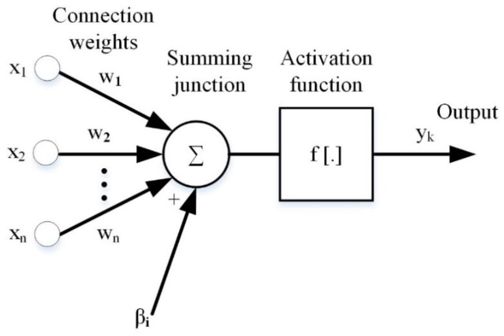
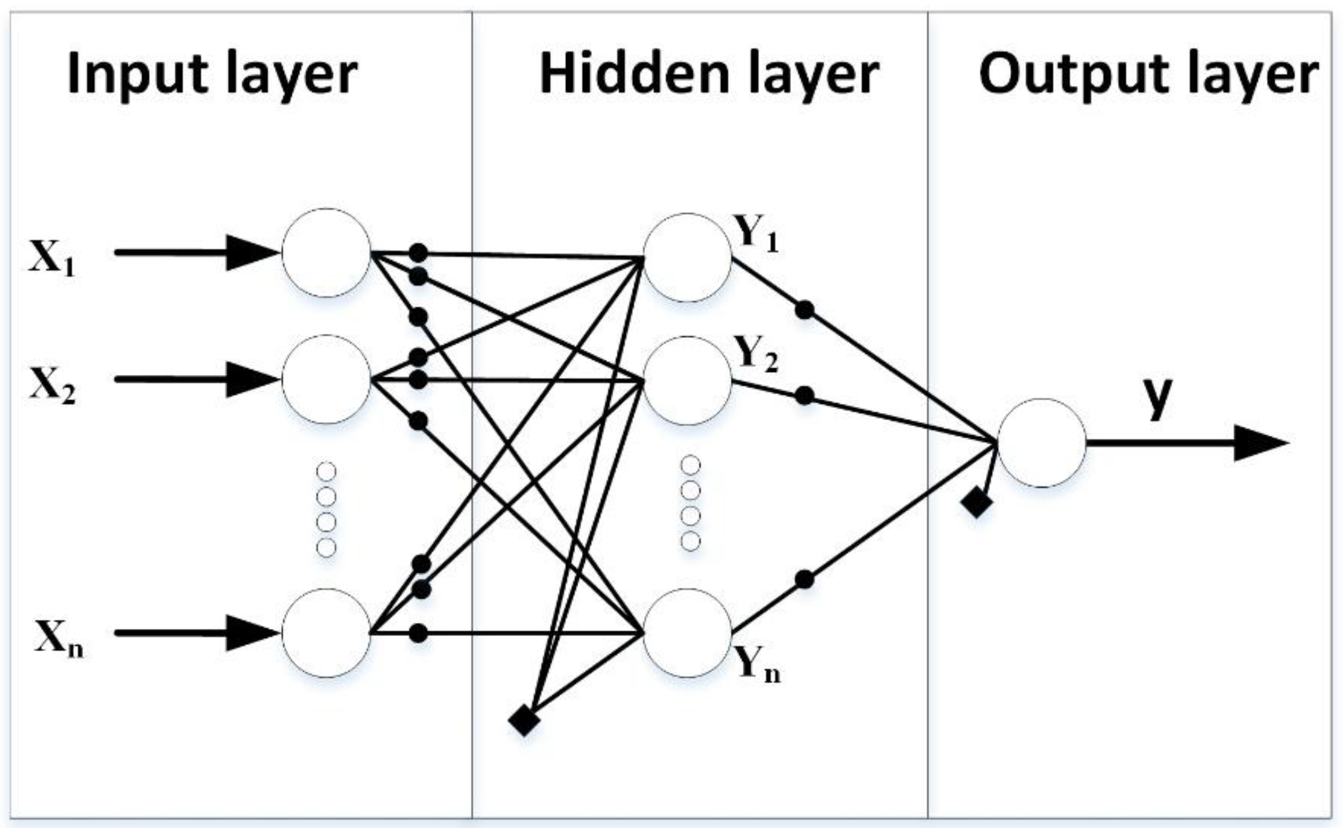
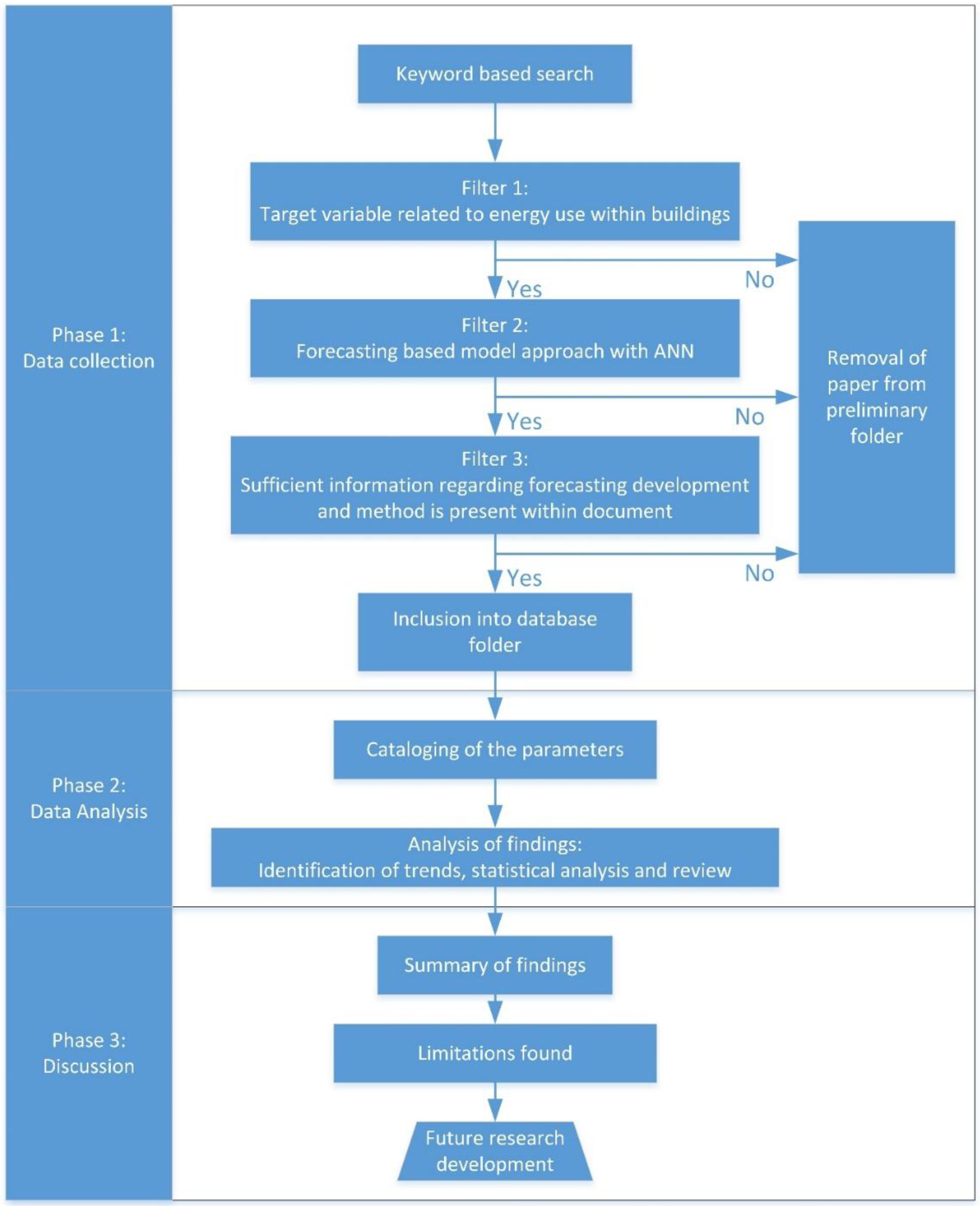
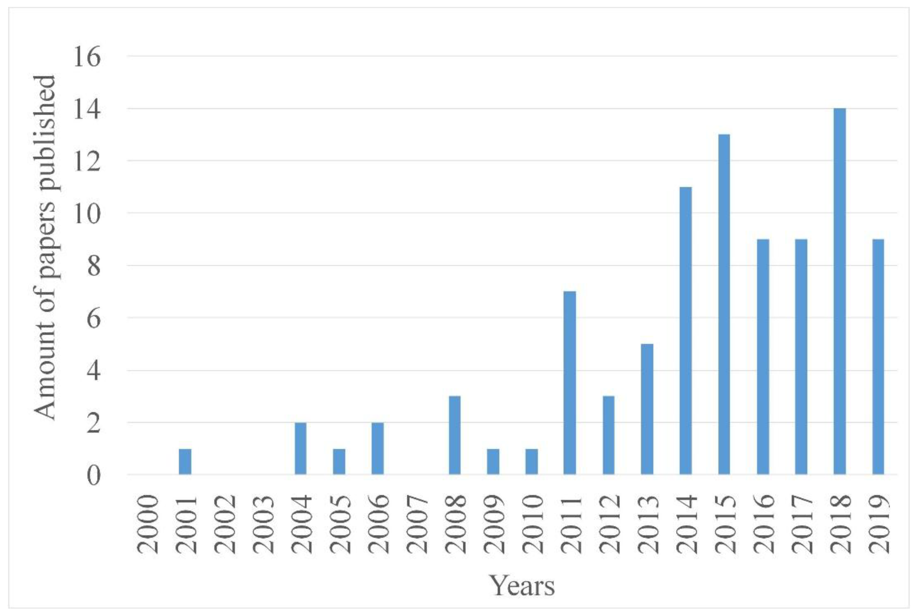
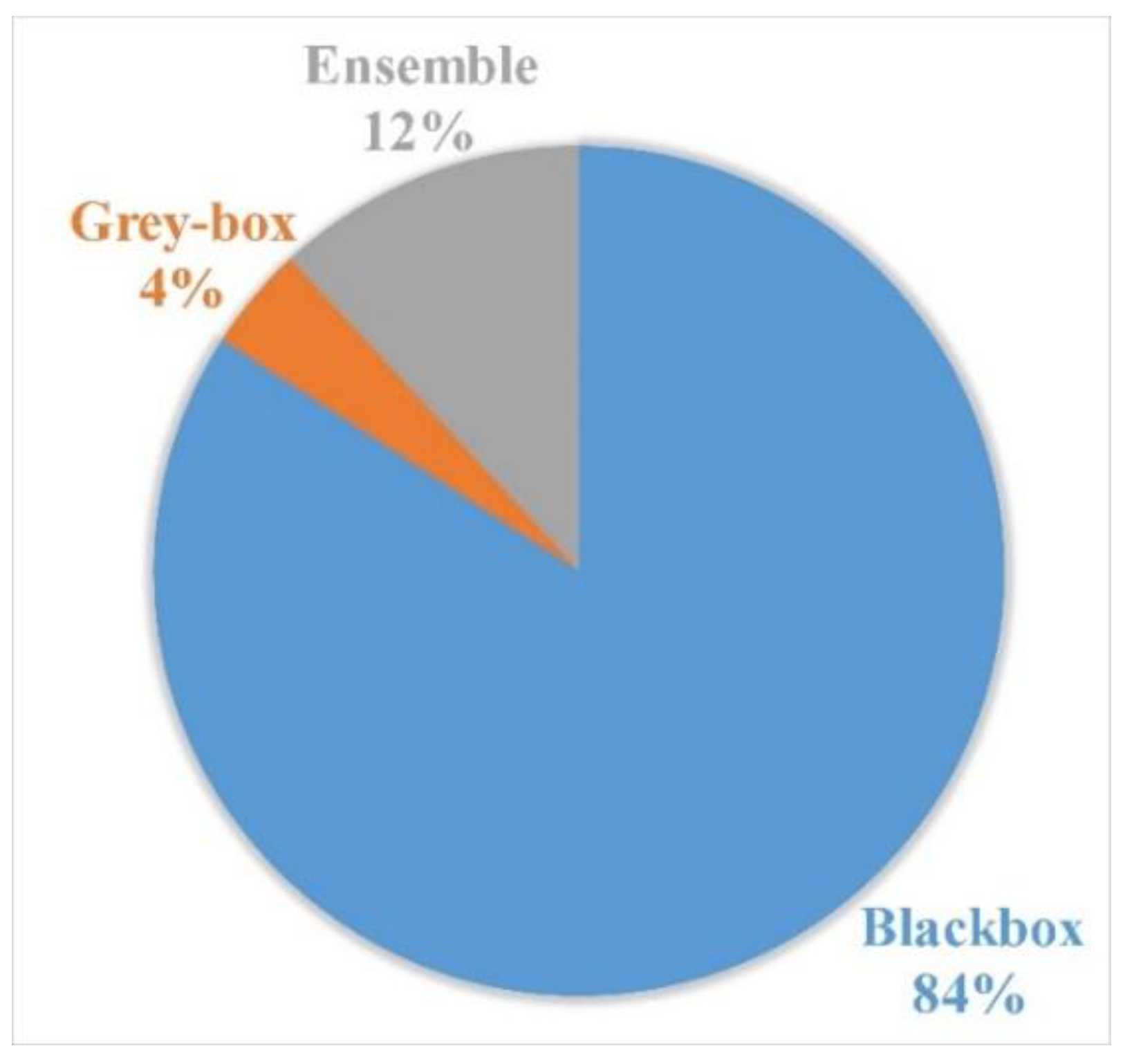
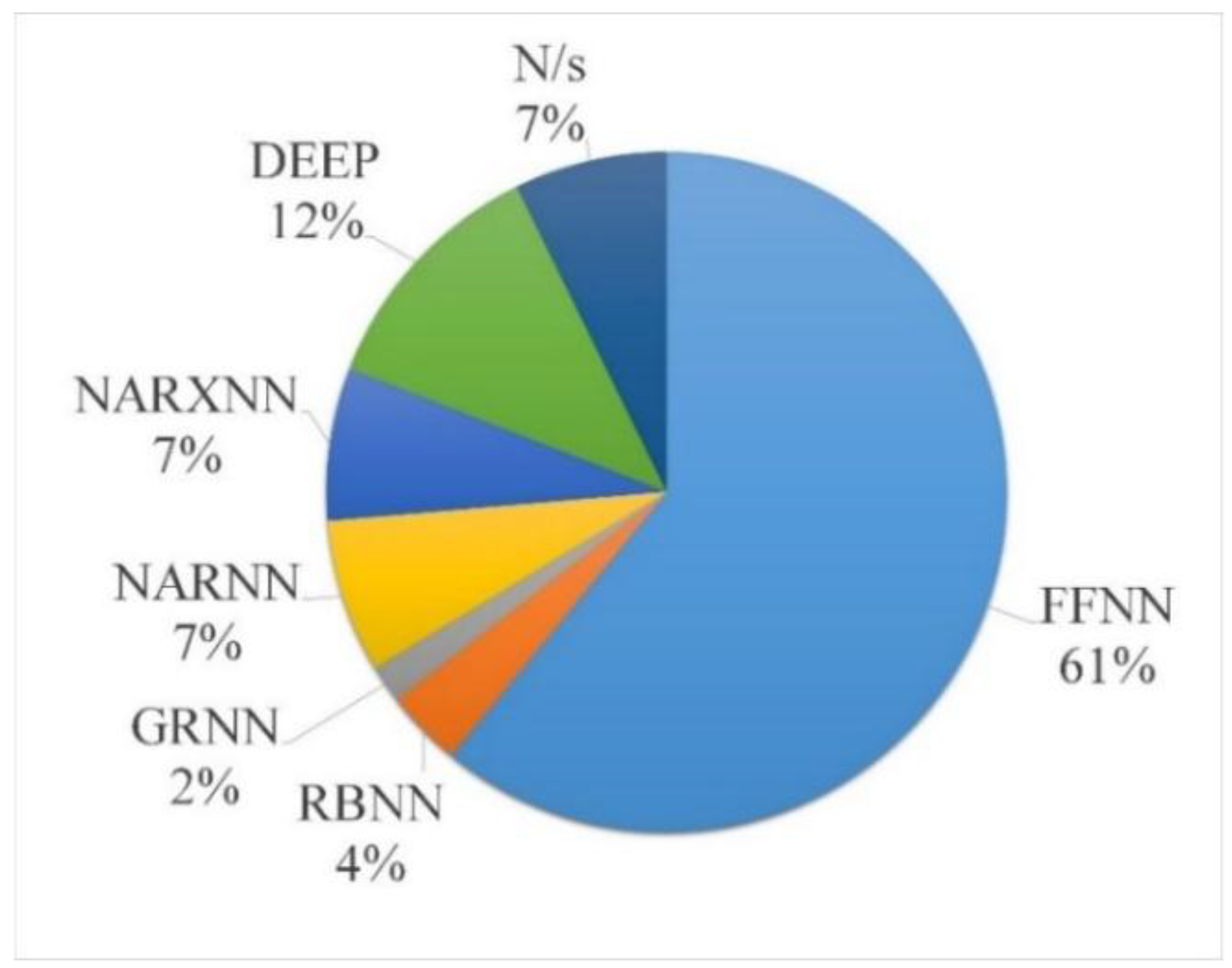
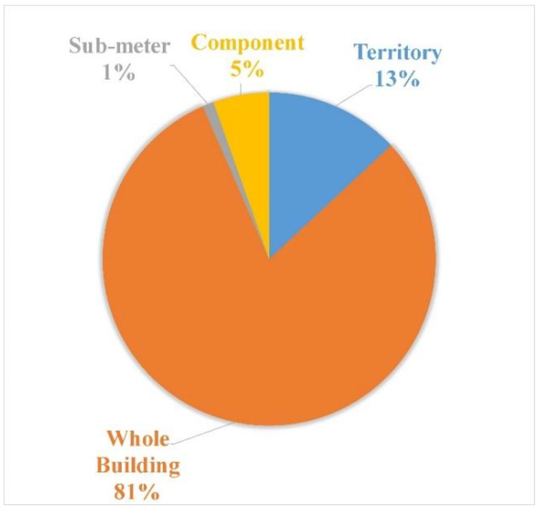
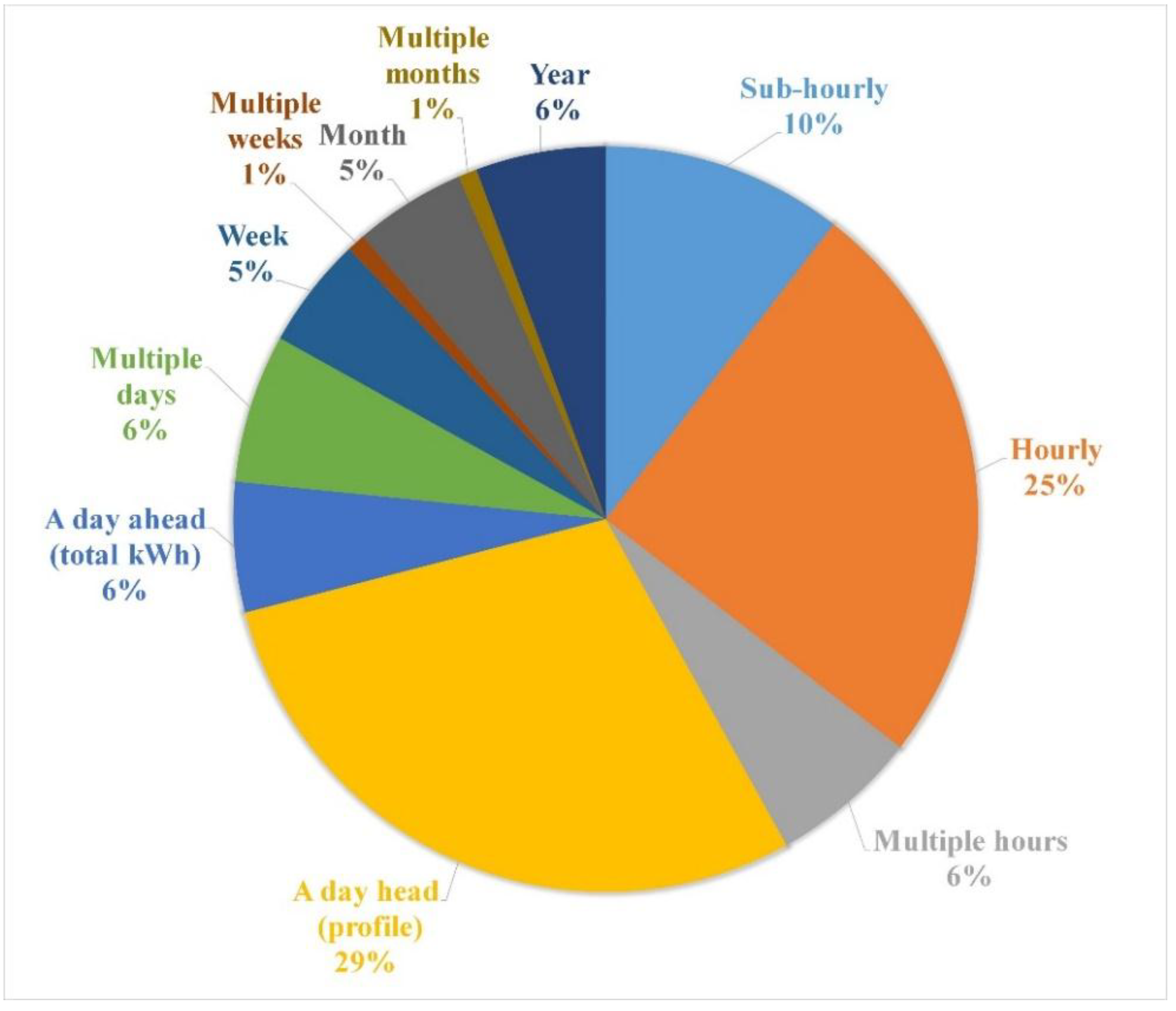
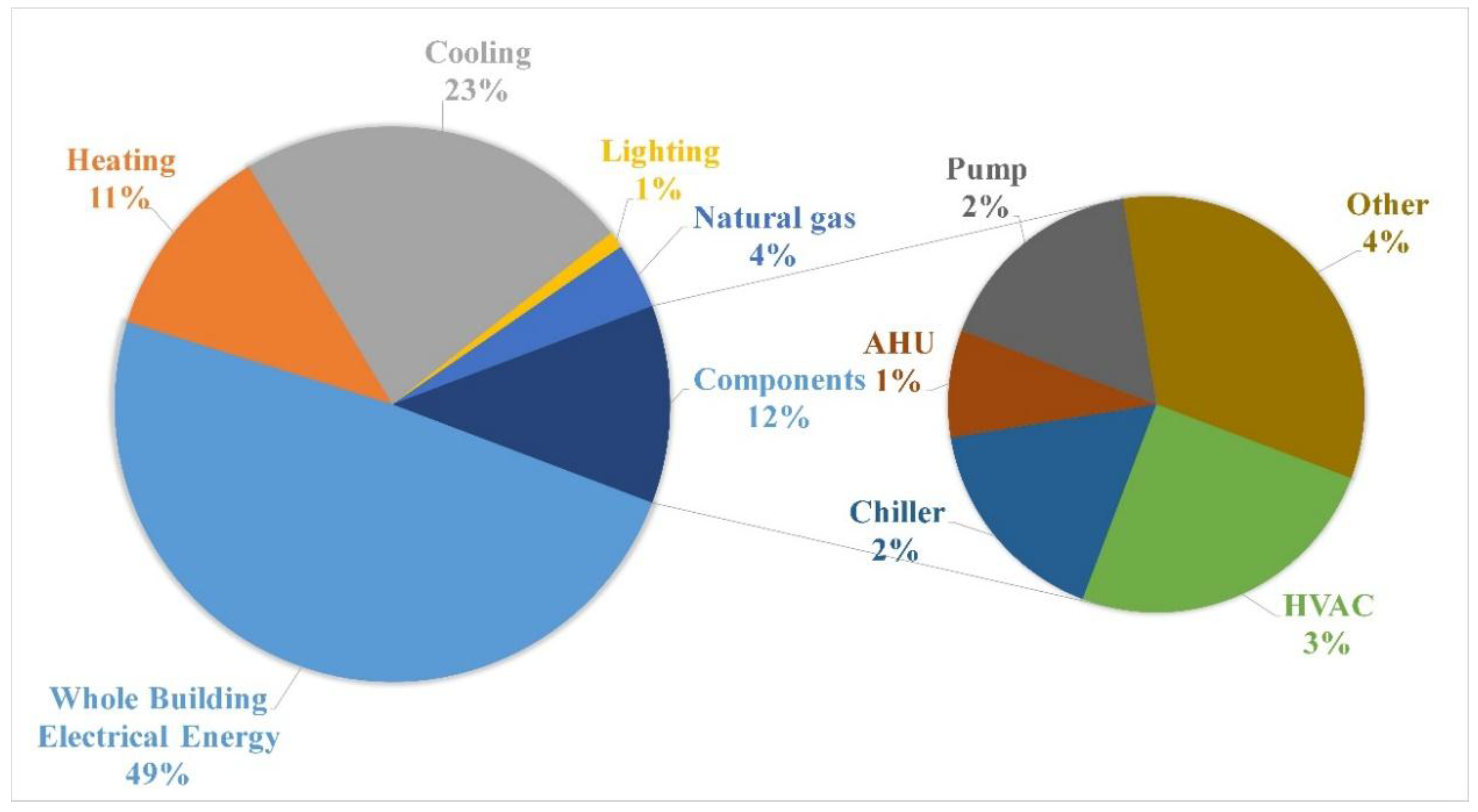
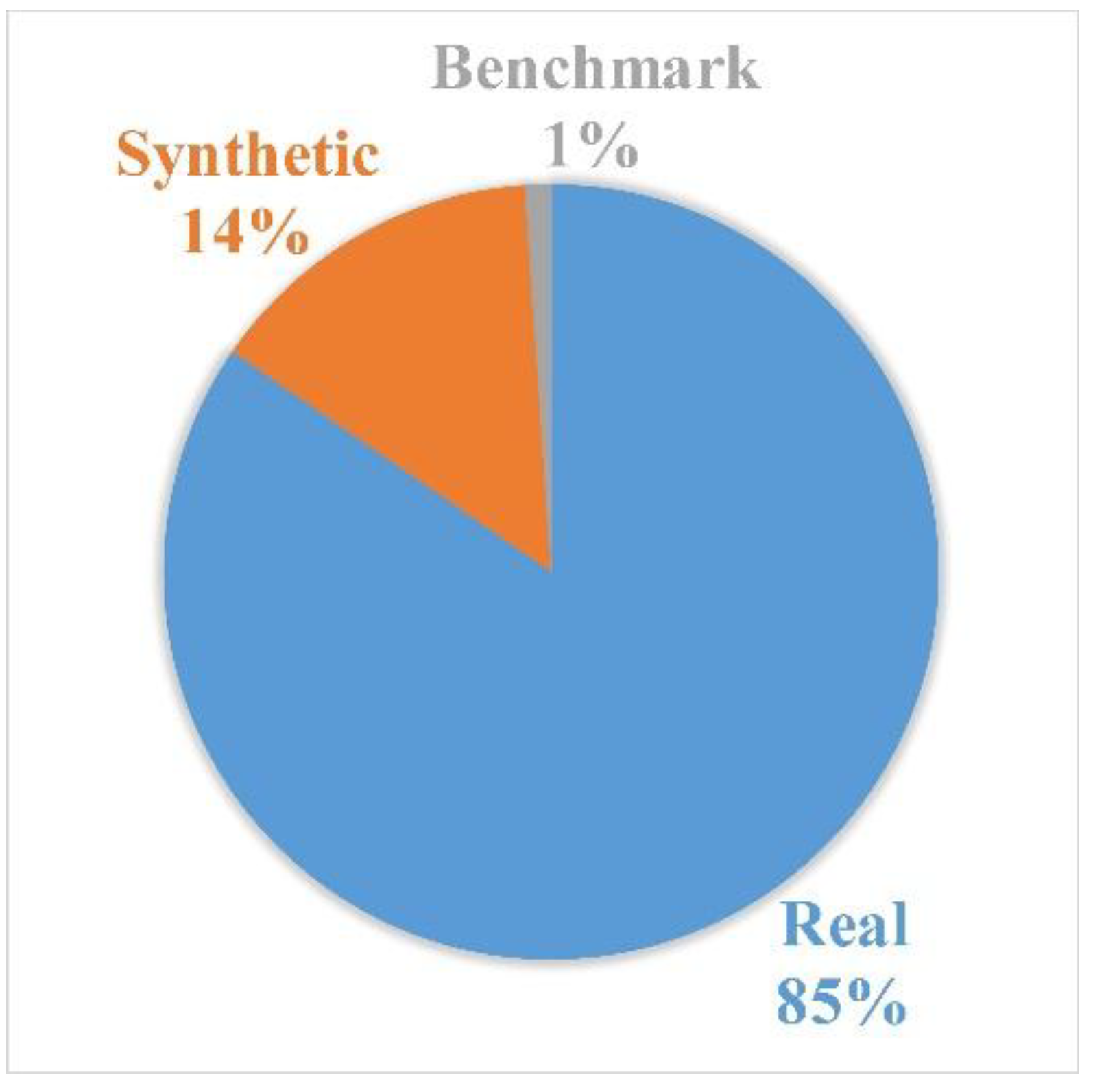
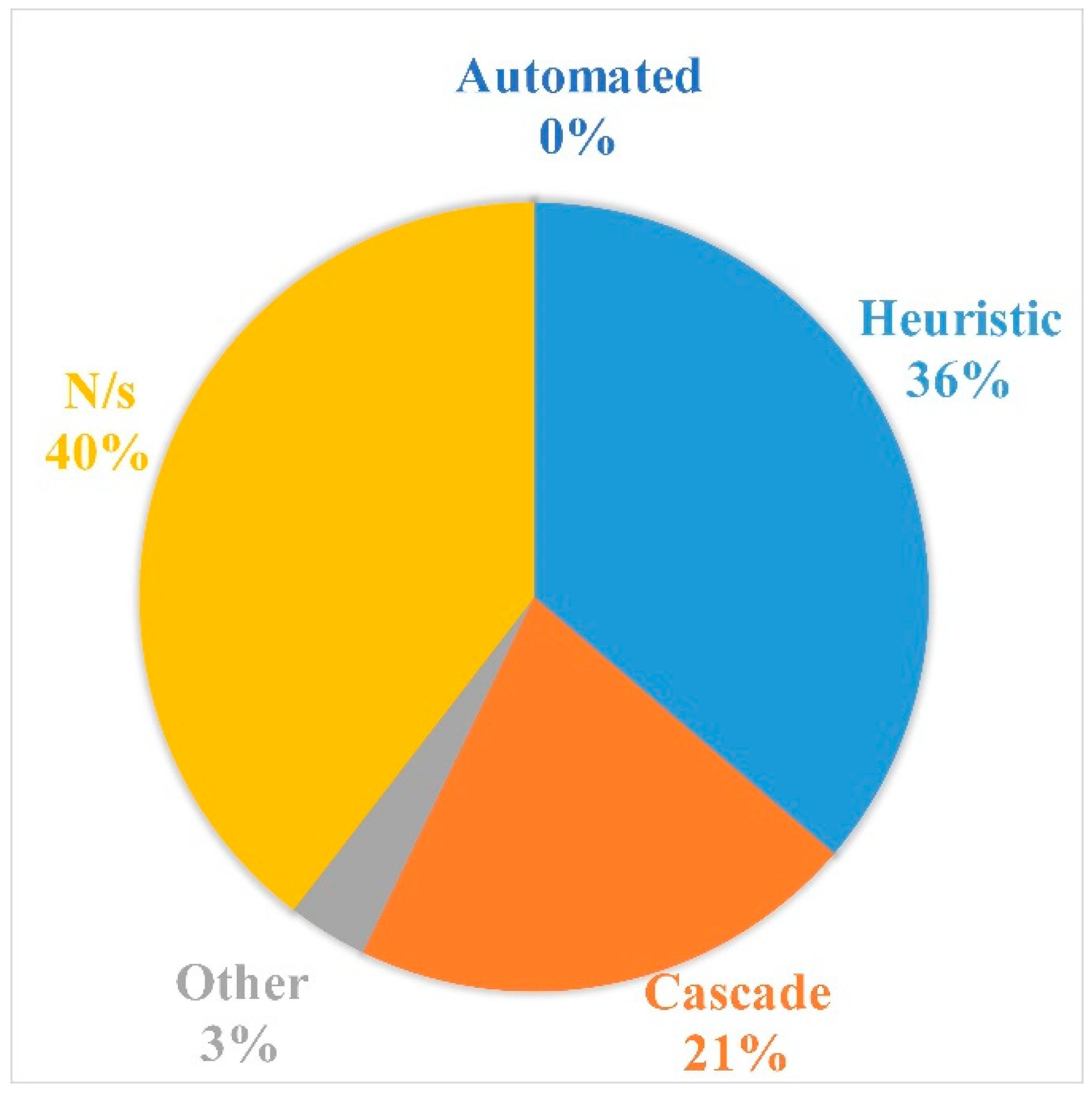
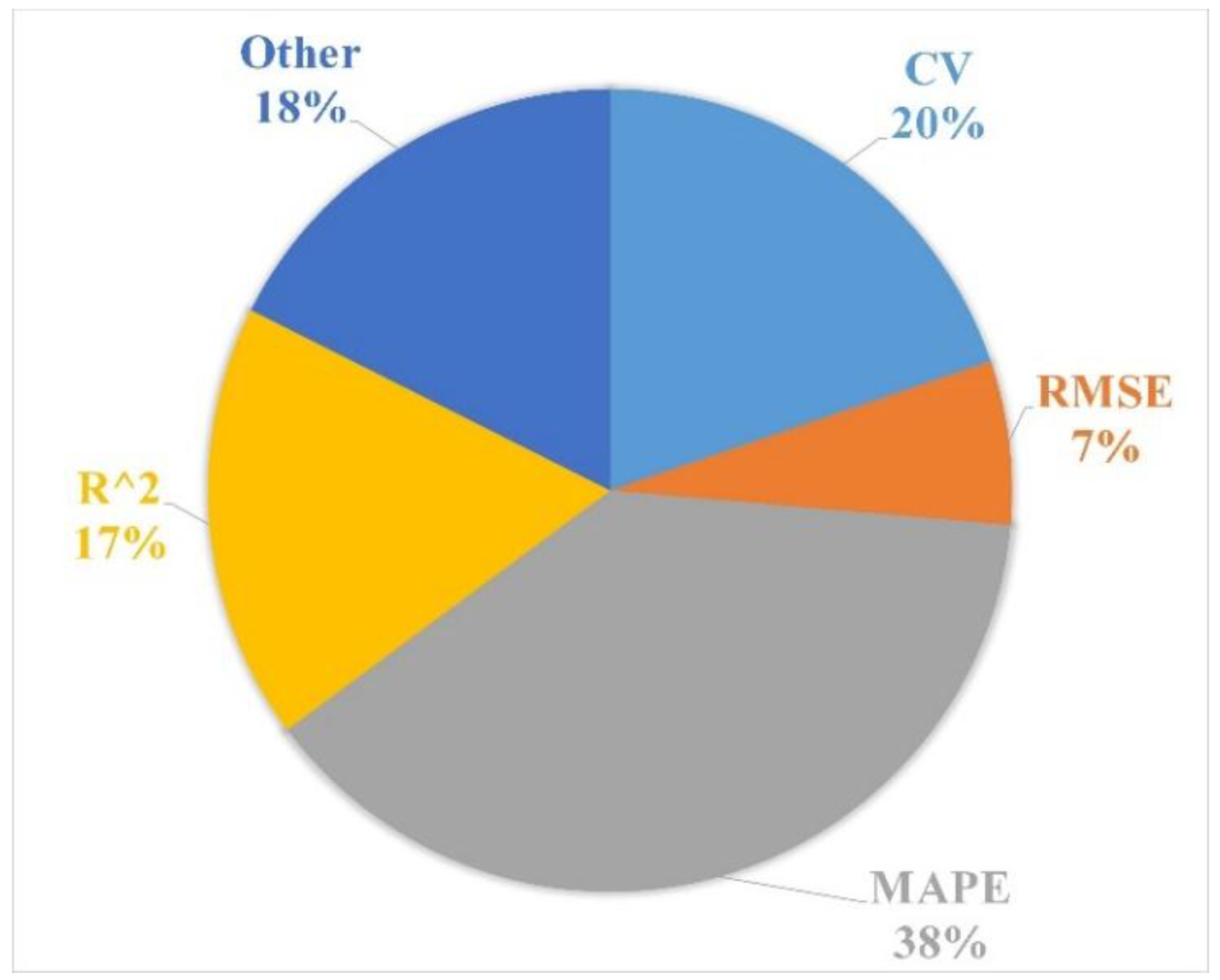
Table 1.
Rule of thumb equations for the estimation of the number of hidden layer neurons.
| Equation | Reference |
|---|---|
| [29,30,31] | |
| [32] | |
| [33,34] | |
| [35,36] | |
| [37,38] | |
| [39] |
Table 2.
Performance range of single step ahead forecasting models.
| Sub-Hourly | |||
|---|---|---|---|
| Paper ID # | Time Step | Forecast Horizon | Error |
| [106] | 15 min | 15 min | 0.001–0.059% (MAPE) |
| [125] | 30 min | 30 min | 0.939–8.34% (MAPE) |
| Hourly | |||
| [125] | 1 h | 1 h | 0.59–19.1% (MAPE) |
| [101] | 1 h | 1 h | 36.5% (MAPE) |
| Multiple hours | |||
| [113] | 12 h | 12 h | 5.03–7.4% (MAPE) |
| Daily (load) | |||
| [56] | Daily | Day ahead | 4.75–6.46% (MAPE) |
| [52] | Daily | Day ahead | 6.63–17.64% (MAPE) |
Table 3.
Performance range of multi-step ahead forecasting models.
| Sub-Hourly | |||
|---|---|---|---|
| Paper ID # | Time Step | Forecast Horizon | Error |
| [57] | 5 min | 40 min | 13.2–14.4% (MAPE) |
| Hourly | |||
| [98] | 15 min | 1 h | 4.5–5.4% (MAPE) |
| [102] | 5 min | 1 h | 8.59–23.86% (MAPE) |
| Multiple hours | |||
| [84] | 1 h | 1–6 h | 7.30–8.48% (CV-RMSE) |
| [64] | 15 min | 1–6 h | 30% (CV-RMSE) |
| Daily (profile) | |||
| [78] | 1 h | 24 h | 1.04–4.64% (MAPE) |
| [85] | 1 h | 24 h | 11.56–11.92% (MAPE) |
| [53] | 15 min | 24 h | 2.59–22.56% (MAPE) |
| [124] | 15 min | 24 h | 36.86–42.31% (MAPE) |
© 2019 by the authors. Licensee MDPI, Basel, Switzerland. This article is an open access article distributed under the terms and conditions of the Creative Commons Attribution (CC BY) license (http://creativecommons.org/licenses/by/4.0/).
Share and Cite
MDPI and ACS Style
Runge, J.; Zmeureanu, R. Forecasting Energy Use in Buildings Using Artificial Neural Networks: A Review. Energies 2019, 12, 3254. https://doi.org/10.3390/en12173254
AMA Style
Runge J, Zmeureanu R. Forecasting Energy Use in Buildings Using Artificial Neural Networks: A Review. Energies. 2019; 12(17):3254. https://doi.org/10.3390/en12173254
Chicago/Turabian StyleRunge, Jason, and Radu Zmeureanu. 2019. "Forecasting Energy Use in Buildings Using Artificial Neural Networks: A Review" Energies 12, no. 17: 3254. https://doi.org/10.3390/en12173254
Note that from the first issue of 2016, this journal uses article numbers instead of page numbers. See further details here.