Towards the Text Compression Based Feature Extraction in High Impedance Fault Detection

Abstract

High impedance faults of medium voltage overhead lines with covered conductors can be identified by the presence of partial discharges. Despite it is a subject of research for more than 60 years, online partial discharges detection is always a challenge, especially in environment with heavy background noise. In this paper, a new approach for partial discharge pattern recognition is presented. All results were obtained on data, acquired from real 22 kV medium voltage overhead power line with covered conductors. The proposed method is based on a text compression algorithm and it serves as a signal similarity estimation, applied for the first time on partial discharge pattern. Its relevancy is examined by three different variations of classification model. The improvement gained on an already deployed model proves its quality.

1. Introduction

Several advantages of Covered conductors (CCs) over Aluminium Core Steel Reinforced (ACSR) medium voltage (MV) overhead lines are leading their gradual replacement especially in a forested and hardly accessible terrain [1,2]. The higher reliability, given by the XLPE insulation system, is the main advantage which leads to no interphase short-circuit in cases of contact of phases [3]. Similarly, the interphase short-circuit does not arise in case a tree branch falls on the CCs phases [2]. On the other hand, the CCs fault detection is a difficult task. The degradation of insulation system is a common problem, especially if CC is used in the forested area. Degradation is usually caused by the contact with surrounding vegetation (tree branch in the most cases). When CC is in a direct contact with any conductive object of a different potential, partial discharges (PD) may appear on the surface of XLPE insulation. This situation is known as high impedance fault (HIF), because PD activity implies only minimal fault current (initial impedance of the fault ranges between tens to hundreds of mega ohms [4]). Such a low value of fault current cannot be detected by standard digital relay protection [1,5]. Methods, able to detect the CC HIF faults, are usually based on evaluation of the signal impulse component (voltage or current). The impulse component of the signal is generated by PDs activity at the fault site; it is visible in the high-frequency band (usually between ${10}^4$ and ${10}^7$ Hz). The measurement approaches based on Rogowski coil [1,6] and the sensor (inductor) placed on the insulation system [5,7] were described in our previous study [8] as well as the issues related to the presence of the background noise interference generated by real environment.

According to the conclusions of several high quality reviews [7,9,10] there are various proposals in the field of partial discharge pattern evaluation aiming at correct feature extraction and classification.

Among the classification approaches, the most families of machine learning models and their modifications were already applied in several successful studies (ANN [10,11], SVM [12], ensemble based approaches [8,13], fuzzy classifiers [14], hidden Markov models [15], etc.). These different models require a different adjustment of their hyper-parameters as well as feature pre-processing to perform some reasonably accurate classification which is not the aim of study of PD-activity but the model optimization itself. As it was concluded in the last available review [9], the most important process for correct PD-activity classification is the extraction of relevant features.

The feature extraction approaches described in available literature varied among the application of basic statistical features [16], the wavelet based decomposition [17], the Fourier transform [18], the fractal theory [19], image based processing, chaos theory [20,21] or representation based on graph structure and adjacency matrices [22,23]. The relevance of features extracted by any selected approach depends on the proper adjustment of the process as well as its ability to handle the external background noise (EBN). Most of the studies attempt to simulate the real conditions by adding the background noise in the observed data. In our case, the data are obtained from real environment where EBN comes from various sources and intensities.

Our aim is to design, develop and evaluate a signal similarity estimation which can be applied as additional feature or classification itself with lowest possible noise-sensitivity and minimal computational costs. The application of compression based similarity is able to fulfill these requirements and on top of that its novelty application on fault detection will be compared with our existing solution based on fundamental features [8]. In case of performance improvement, the combined solution will be deployed as a HIF detector on the real environment.

2. Experiment Design

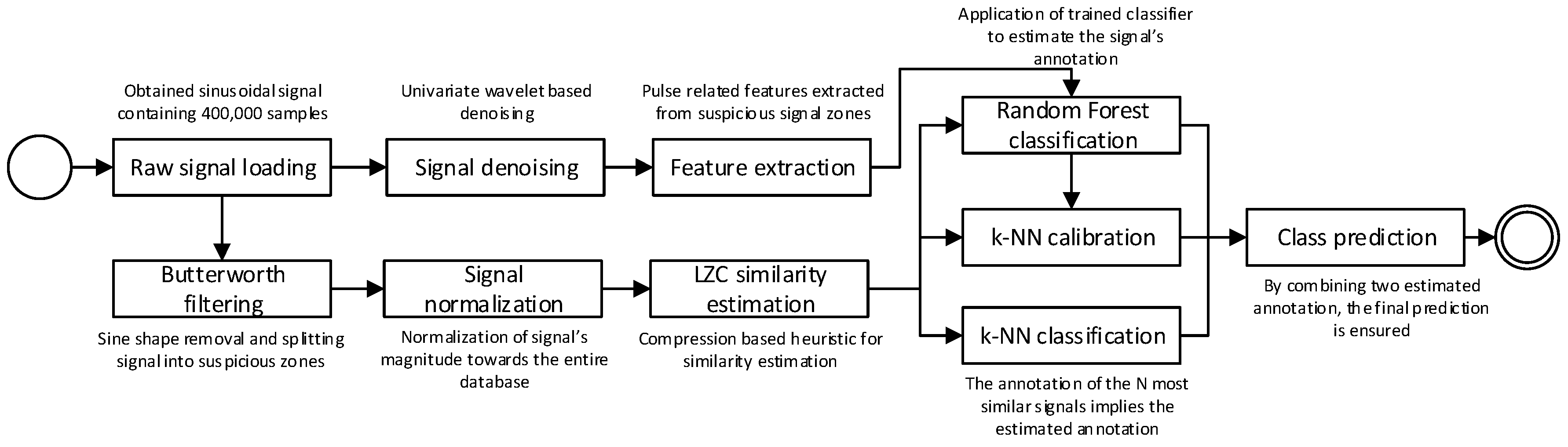
The experiment, described in this paper, contains several phases and a novelty application of compression based similarity function, which is evaluated in three different regimes (classification variations). The estimated signal similarity value is applied in simple k-NN classification, as an additional input value for the random forest algorithm and weighted k-NN classification which serves as calibration of RF predictions. The UML block scheme of the experiment is depicted in Figure 1.

2.1. Data Acquisition

Gathering of the data was performed in real environment, forested or hardly accessible terrain, where the metering device was deployed on an overhead line. The locations of deployment will not be published due to the security reasons, but currently our project maintain more than 20 different deployments in several areas of Czech republic.

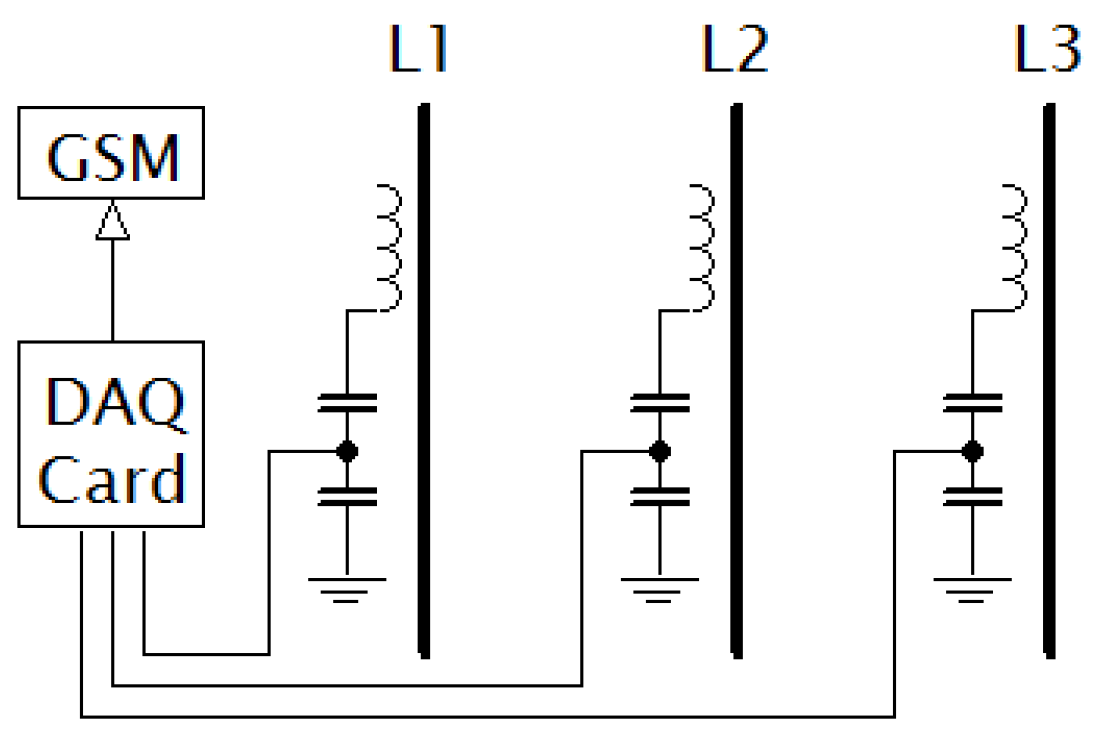
The metering device uses single layer inductor (SLI) as a voltage sensor. SLIs are mounted on the surface of the CC (one inductor per phase). Each SLI is connected to the capacitance divider, output of this divider is connected to the data acquisition card. Control unit of whole detector triggers signals measurement in a scheduled time (see schema in Figure 2).

Acquired signals are sent through GPRS module to the database server for further data processing and evaluation. The detailed description of a physical platform was brought in [5].

The measurement acquires signals in a length of 20 ms every hour on all three phases (one period of 50 Hz power grid frequency is equal to 20 ms). This results in three signal time series. Each of them contains 400,000 samples with 20 MS/s sampling rate. Those signals are sent into our database where are stored for further analysis. For the purpose of this experiment, 500 signals were selected in order to cover all typical kinds of noisy signals accompanied by the majority of the obtained fault signals. This dataset was randomly shuffled and split into training and testing parts (75% to 25%).

Every fault observed on overhead lines is compared with stored data such as each signal is labeled by an human expert. The labels are assigned to the signals based on visual pattern they contain. In case of the fault presence, the malfunction on the overhead lines is double checked by maintaining service operators. Maintenance service operators provides us all detailed information about the fault, like the distance, type of fault (line-to-ground or line-to-line), cause of fault, clearing time etc. Seven different labels are defined to differentiate fault and non-fault signals. Six of them describes the specific kind of faults as it is stated in

Table 1. Annotations of 7 typical signals of PD patterns, defined by our previous study [20].

Index	Annotation Describtion
an0	signal indicating no fault on the covered conductor (CC)
an1	weak appearance of the event when a tree or branch is in contact with CC and through that the CC is connected to the ground
an2	weak appearance of the event when a branch is in contact with multiple CCs and through that the phases are interconnected
an3	interruption of the CC fault
an4	incorrect behavior due to degradation of the CC insulation system
an5	strong appearance of the event when a tree or branch is in contact with CC and through that the CC is connected to the ground
an6	strong appearance of the event when a branch is in contact with multiple CCs and through that the phases are interconnected

.

2.2. Background Noise

Unlike the laboratory environment, signals obtained from a real power lines contain high level of background noise. Discrete spectral interference (DSI) is present in all of the acquired signals in a form of radio broadcasting signals (overhead power line act as a long wire antenna). DSI noise magnitude is very variable and depends on time of the day, weather season and ionospheric conditions. High level of DSI covers PD pattern in obtained signals, making it difficult to detect. During the acquisition of data for this experiment, the highest observed DSI level reached peak value of 0.29 V (data acquisition card range is 0.5 V, so the DSI noise can reach 50 percent of its range). Another issue is pulse interference (PI), which generates impulse component in acquired signals. Such pulses have no relation with XLPE insulation, they are caused by other type of discharges, switching operations, atmospheric discharges or they can be induced into the measuring system due to electromagnetic coupling. PI pulses can be misinterpreted as PD pattern.

2.3. Denoising and Feature Extraction

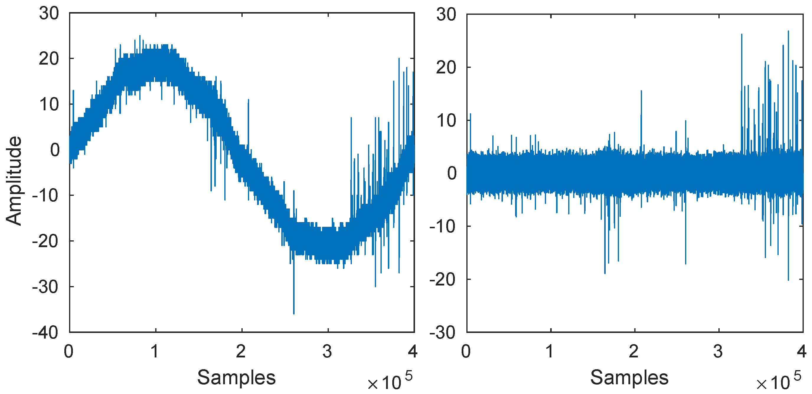
Raw signals were synchronised the way mentioned previously. All of them starts from zero and has the same sine shape in order to correctly select the relevant signal parts. In order to suppress the noise interference, the butterworth filter was applied. The effect of BF application with defined cut-off frequency 50Hz is depicted on Figure 3. This was followed by DWT based denoising which removed the majority of small pulses. Those that remained were examined by our feature extraction procedure.

The pulse related features are considered as the most relevant indications of partial discharge activity according to the available literature and our previous experiments. With respect to this fact, we applied the feature extraction from our previous study [8], where their relevance was on PD detection accuracy quantified. The process extracts signal pulses and computes their count and the mean/max/min of their width and magnitude. This process also involves the cancellation of false-hit pulses. False-hit pulses are not generated by the PD activity, but they come as a result of the noise interference. Set of rules, defined by expert’s adjustment, contained several key characteristics (see in

Table 2. Settings applied in denoising and feature extraction from previous study [8]. * IG stands for information gain criteria.

Parameter	Value	Meaning
maxDistance [samples]	10	maximal distance between pulse and its opposite pulse
maxHeightRatio [%]	25	ratio of amplitudes between suspected pulse and its opposite one
maxHeight [%]	100	maximal amp. of the pulse compared to the amp. of sine
maxTicksRemoval [samples]	500	number of pulses suppressed after the opposite pulse
mother wavelet	db4	selected wavelet for DWT decomposition
level of decomposition	1	detailed coefficients were not decomposed again
thresholding method	hard	values under the threshold were set to zero

). This set of rules is based on a fundamental knowledge of PD a pulse shape and can be applied only on signals, acquired from power lines with previously described detector. PD pulse cannot be measured directly and the response of sensor is affected by the measuring system and tested object. This is why this set of rules will probably not work with any other type of measuring sensors or with different objects under test.

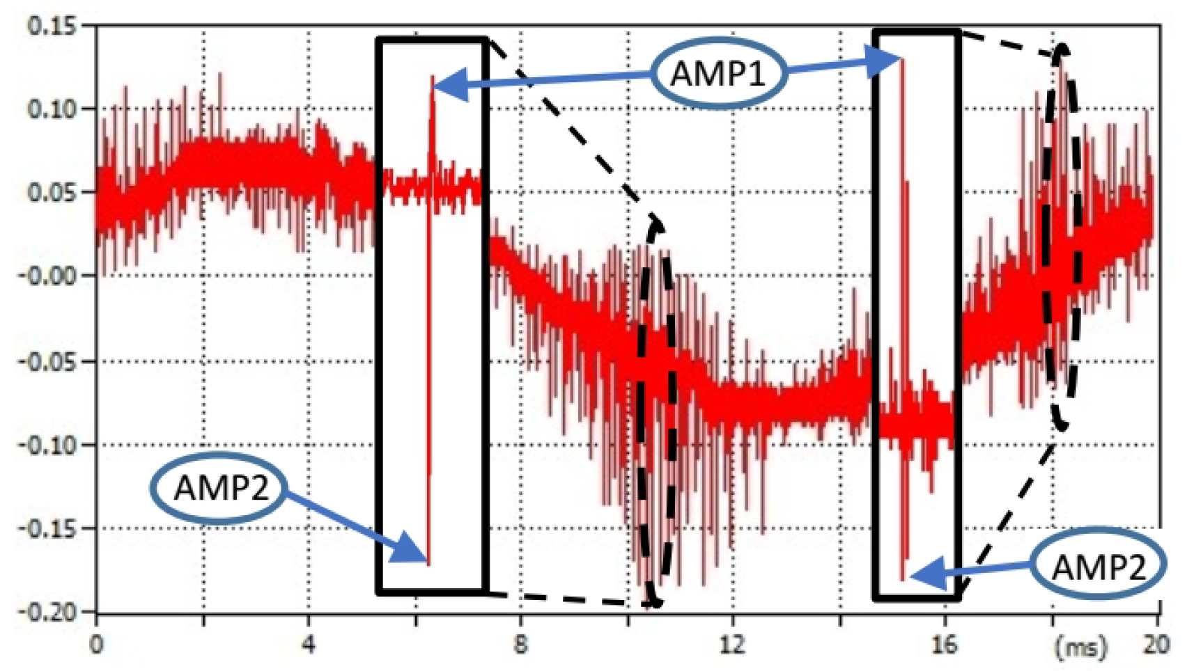
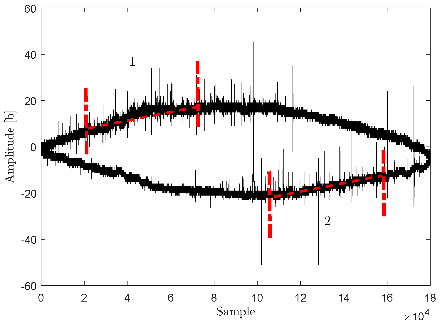
According to [24], the charge of surface or void PD pulse is mostly positive polarity in one half cycle and negative in the other one. This matches our observations, as it can be seen in in Figure 4. This signal was acquired during the line to ground fault. During the rising slope, polarity of PD pulse is positive ($\mathrm{AMP}1\gg \mathrm{AMP}2$). During the falling slope, polarity of PD pulse is negative ($\mathrm{AMP}1\ll \mathrm{AMP}2$).

Pulses with almost equal magnitudes ($\mathrm{AMP}1\approx \mathrm{AMP}2$) are usually non-related to the CC insulation system and can be considered as false-hits. These pulses can have their origin in background noise or it can be propagated into the measuring system thanks to the inductive and capacitance coupling of a power line conductors. Example of such situation can be seen in Figure 5. There was no fault on this particular phase, but despite this fact there are pulses in acquired signal. They were induced into the measuring system through the electromagnetic coupling between conductors (there was line to ground fault on the other phase, signal was acquired during the ground fault recorded in Figure 4). The ratio of magnitudes “AMP1” and “AMP2” differs from pulses in affected phase, see the detail in Figure 5.

Based on our observations (there are already several hundred thousands of acquired signals in our database), the false-hit peak is typical by its high initial magnitude “AMP1” (magnitude that cannot be achieved by the PD activity, even in a close distance of a detector), or by the close presence of pulse with the opposite magnitude “AMP2” (in defined closeness “maxDistance” and defined amplitude ratio), or by the regular spacing or by the areas of signal where it appear. Each pulse triggers a transient. If any pulse is identified as a false-hit pulse, a certain number of samples, followed by this pulse, are neglected. This prevents the misinterpretation of pulses from the following transient as a PD event.

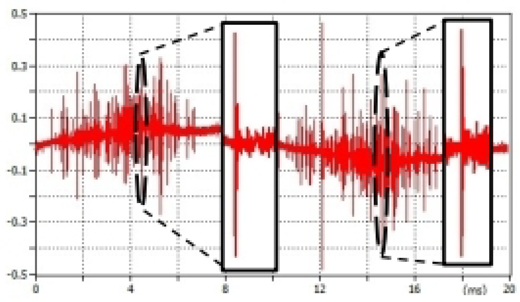
The feature extraction process is not executed on the entire length of the acquired signal. There are only several parts with higher probability of PD activity appearance, because it is generated by the surface and void discharges of a XLPE insulation with specific phase resolved diagram patterns [24]. Random pulse interference can appear in any part of the signal and it can be misinterpreted as PD activity. The smaller portion of a signal is analyzed, the lower is probability of a noise pulse presence in analyzed part. It is also necessary to avoid parts around maximum/minimum of the carrier sine wave, because they often contains corona discharge pulses. This is why only parts with high probability of PD occurrence and low probability of other type of discharges appearance are analyzed (see Figure 6). The relevance of these parts was examined in [8]. The influence of insulation aging on this relevance is possible, but we are unable to analyze it yet (the oldest monitored power line was constructed six years ago and does not show any sign of aging yet). The same signal areas are applied for fundamental feature extraction as well as for LZC processing.

Measured signals are not starting at the same position in the sinusoidal shape, therefore they need to be synchronised. They all need to posses a shape of increasing wave at the beginning, crossing the zero line in the middle when decreasing into its negative part and then increasing back towards the zero. Synchronization of a noisy signals was performed making use of extracting of an approximated shape from wavelet decomposition and estimation of global extremes. Based on them, the signals were cut into pieces and concatenated back to form this shape.

2.4. Measuring the Similarity of Input Data Using LZC

The comparison of the LZ sequences lists is the main task in our approach. The lists are compared to each other. The main property for comparison is the number of common sequences in both lists of two input data. This number is represented by the $sc$ parameter in the Equation (1), which is a metric of similarity between LZ sequences lists.

$$SM=\frac{sc}{min(c_1,c_2)}$$

(1)

where:

• $sc$ is count of common LZ sequences in both lists.
• $c_1,c_2$ is a count of LZ sequences in list of the first or the second sample.

The $SM$ value is in the interval between 0 and 1. If $SM=1$, then the two list are equal, but if the value of $SM=0$, then the samples are totally different.

2.5. Classification

As it was mentioned previously, the application of LZC similarity is applied in three different variations of classification in order to examine its relevancy. A product of LZC is represented by two similarity matrices (each one is computed on one selected signal area), which serve in all of those variations. For simplicity, the k-nearest neighbors (k-NN) algorithm [25] was applied to perform classification based on LZC similarity values.

• k-NN is used to predict the class of observed signal as the major class of its neighbors. The neighborhood is established as a closeness of observations according to the similarity matrix (higher similarity among observations means higher closeness). The final prediction comes as an average of two sub-predictions computed on both similarity matrices.
• k-NN computes two average values of nearest neighbors annotations (one from each similarity matrix) and passes them into RF as another input values. The model is than trained and evaluated for classification performance.
• weighted k-NN is applied for calibration of RF classification. Neighbors’ classes are put together with predicted class from RF and the result is given by the majority. The weighted version of k-NN is applied because of the different character of voting entities. The optimization of weights is simply ensured making use of Differential evolution (DE) [26], which turns this process into supervised classification.

Adjustment of the applied algorithms as well as data processing is described in following section.

3. Theoretical Background

The described experiment uses advanced techniques of data, especially signal, processing, briefly reviewed in the following sections.

3.1. Butterworth Filtering

The Butterworth filter (BF) [27] has been commonly used in gait analysis applications. The only parameter which needs to be set by the user, is a cut-off frequency (when assuming constant order and number of passes). BF has a magnitude response that is maximally flat in the passband and monotonic overall. This smoothness comes at the price of decreased rolloff steepness. The amplitude response of n-th order BF is given as follows:

$$\frac{V_{out}}{V_{in}}=\frac{1}{\sqrt{1+{(f_c/f)}^{2n}}},$$

(2)

where:

• f is frequency at which calculation is made,
• $f_c$ is the cut-off frequency, i.e., half power or -3dB frequency,
• $V_{in}$ is the input voltage,
• $V_{out}$ is the output voltage,
• n is the number of poles.

The poles of a BF with cut-off frequency $\omega c$ are evenly-spaced around the circumference of a half-circle of radius $\omega c$ centered upon the origin of the s-plane.

The equation can be rewritten to give its more usual format. Here $H\left(j\omega \right)$ is the transfer function and it is assumed the filter has no gain, i.e., it is not an active filter.

$$\left|H\left(j\omega \right)\right|=\frac{1}{\sqrt{1+{({\omega }_c/\omega )}^{2n}}},$$

(3)

where:

• $H\left(j\omega \right)$ is transfer function at angular frequency $\omega$,
• $\omega$ is angular frequency and is equal to $2\pi f$,
• ${\omega }_c$ is cutoff frequency expressed as an angular value and is equal to $2\pi f_c$

3.2. External Background Noise Suppression

The major part of noise interference is aimed to be suppressed making use of a denoising procedure. In our case, the discrete wavelet transformation with coefficient thresholding is followed by the signals reconstruction. It is supposed to remove the noise related pulses with lower amplitude and higher frequency of occurrence. The hard-thresholding approach sets to zero all coefficients values under the defined threshold. The applied mother wavelet is selected according to the energy computed from obtained coefficients (see in Equation (4)) [28].

$$E_a=\frac{{\displaystyle \sum _k}{a}_{j,k}^2}{{\displaystyle \sum _k}{a}_{j,k}^2+{\displaystyle \sum _k\sum _j}{d}_{j,k}^2}$$

(4)

The threshold value T is than estimated according

$$\sigma =\frac{1}{0.6745}\times MAD\left(c_d\right);T=\sigma \sqrt{2log\left(N\right)}$$

(5)

is the noise estimation, c stand for the vector of detail coefficients and N is the size of that vector. The energy is computed from sums of approximation a and detailed d coefficients on a j-th level of decomposition over all K coefficients. The MAD operation mentioned in the threshold estimation stands for the mean absolute deviation.

3.3. Lempel-Ziv Complexity Similarity Estimation

Lempel-Ziv complexity (LZC) and derived LZ algorithms have been extensively used to solve information theoretic problems, such as coding and lossless data compression. In recent years, LZ has been widely used in biomedical applications to estimate the complexity of discrete-time signals [29]. The input data must be transformed into a finite symbol sequence. For example in the context of signal analysis, typically the discrete-time signal is converted into a binary sequence. By comparison with the threshold $T_d$, the signal data ($X\in (x_1,x_2,\cdots ,x_n)$) are converted into a 0–1 sequence P as follows [30]:

$$P=s_1,s_2,\cdots ,s_n$$

(6)

where

$$s_i=\left\{\begin{array}{cc}0\hfill & \mathrm{if}{x}_i<T_d,\hfill \\ 1\hfill & \mathrm{otherwise}\hfill \end{array}\right..$$

(7)

Usually, the median is used as the threshold $T_d$ because of its robustness to outliers [29].

The LZC for sequences of finite length was suggested by Lempel and Ziv in [31]. It is a non-parametric, simple-to-calculate measure of complexity in a one-dimensional data. LZC is related to the number of distinct sequences of input data and the rate of their recurrence along the given input sequence [32]. The larger values of LZC are corresponding to more complexity in the data.

It has been applied to study the brain function, detect ventricular tachycardia, fibrillation, and EEG [30]. Also, LZC has been applied to extract complexity from mutual information time series of electroencephalography (EEG) data in order to predict response during isoflurane anesthesia with artificial neural networks in [33]. The complexity measure can be estimated using the following algorithm [31]:

• Let S and Q denote two sequences of P and $SQ$ be the concatenation of S and Q, while sequence $SQ\pi$ is derived from $SQ$ after its last character is deleted ($\pi$ means the operation to delete the last character in the sequence). Let $v\left(SQ\pi \right)$ denote the vocabulary of all different sequences of $SQ\pi$. At the beginning, $c\left(n\right)=1$, $S=s\left(1\right)$, $Q=s\left(2\right)$, therefore, $SQ\pi =s\left(1\right)$.
• In general, $S=s\left(1\right),s\left(2\right),\cdots ,s\left(r\right)$, $Q=s(r+1)$, then $SQ\pi =s\left(1\right),s\left(2\right),\cdots ,s\left(r\right)$; if Q belongs to $v\left(SQ\pi \right)$, then Q is a sequence of $SQ\pi$, not a new sequence.
• Renew Q to be $s(r+1)$, $s(r+2)$ and judge if Q belongs to $v\left(SQ\pi \right)$ or not.
• Repeat the previous steps until Q does not belong to $v\left(SQ\pi \right)$. Now $Qts=s(r+1),s(r+2),\cdots ,s(r+i)$ is not a sequence of $SQ\pi =s\left(1\right),s\left(2\right),\pi ,s(r+i-1)$, so increase $c\left(n\right)$ by one.
• Thereafter, S is renewed to be $S=s\left(1\right),s\left(2\right),\cdots ,s(r+i)$, and $Q=s(r+i+1)$.

These procedures have to be repeated until Q is the last character. At this time, the number of different subsequences in P—the measure of complexity—is equal to $c\left(n\right)$. In order to obtain the complexity measure of the input data which is independent of the sequence length, $c\left(n\right)$ must be normalized. If the length of the sequence is n and the number of different symbols in the symbol set is $\alpha$, it has been proved that the upper bound of $c\left(n\right)$ is given by [34]

$$c\left(n\right)<\frac{n}{(1-{ϵ}_n){log}_{\alpha }\left(n\right)}$$

(8)

where ${ϵ}_n$ is a small quality and ${ϵ}_n\to 0,n\to \infty$.

In our experiment, we do not deal with the measure of the complexity. Based on the individual subsequences, we create a list of the LZ sequences. One list is created for each data file with turtle commands of the compared files.

LZC analysis is based on a coarse-graining of the measurements, before the calculation of the complexity measure. The signal must be transformed into a finite symbol sequence. In this study, we have converted the captured signal into bytes. The signal is presented as a series of consecutive bytes P. The series P is scanned in a direction from left to right and the complexity counter is increased by one unit every time a new sequence of consecutive bytes is encountered. The complexity measure can be estimated using the algorithm described in [31,33]. LZC can be described on a brief example of a binary encoded input. For example: if the input is 000110100100010 and LZ algorithm is applied, the sequence 0, 001, 10, 100, 1000, 101 is obtained as a result.

In our experiments, we do not deal with complexity measure of LZ [31,33]. From the individual obtained sequences, a list is created. List of LZ sequences is independent of its order. One list is created for each data part of the captured sample.

3.4. Random Forest Based Classification

As a part of our previous study reconstruction [8], the application of supervised learning model is necessary in order to obtain a classification model. The random forest (RF) was used in this purpose. The model proposed by Breiman in 2001 [35] gained wide attention and was successfully applied in many machine learning studies [36,37]. The core idea of the algorithm is focused on the application of an ensemble of CART-like tree classifiers [38] learned on the randomly selected and replaced observations (bagging of the dataset). This increases the overall complexity of the algorithm which is supposed to reduce the variance and keep the bias as low as possible.

4. Adjustments and Results

The first half of the experiment reproduces our previous study [8] which implies a necessity of the same adjustment using in case of denoising, feature extraction and random forest classification. A brief summarization of applied parameters is listed in

Table 3. Settings applied in RF classification.

Parameter	Value	Meaning
number of trees	200	CART-like trees applied in random forest algorithm
features per tree	all	set up for bagging model in random forest
samples per tree	all	set up for bagging model in random forest
splitting criteria	IG	selection criteria in DT algorithm for node creation

. From all proposed combinations of the classification model, we applied the expert based adjustment with all noise-suppressing modules [8]. This model is clearly based on fundamental knowledge and reflects the relevancy of applied signal features, therefore it serves well for comparison with the extended model by LZC.

As it was mentioned previously, LZC is a parameter free method, which serves as unsupervised part and also as the extraction of an additional potentially relevant features. The only adjustable parameter can be the size of the dictionary applied in compression. In our case, double values are encoded into byte values in the range [−128, 127] which are further compressed. The application of entire byte range was the only adjustment of the LZC algorithm. This step also served as a normalization of input data into one common range for all observed signals. The computation of LZC was performed twice per each signal, on each selected signal’s area separately, therefore two similarity matrices were obtained.

The k-NN based classification simply took 6 nearest neighbors on each similarity matrix and averaged their output classes. The result came up as average from both matrices predictions (LZC in

Table 4. Performance evaluation of all applied variations of classification model.

[%]	RF [8]	LZC	LZC, RF	RF, LZC
ACC	89.3	75.8	91.0	85.0
PREC	84.1	42.0	86.2	64.5
REC	55.6	68.7	64.1	58.1
F-score	66.1	52.1	73.5	61.1

). Those features (LZC similarity from the first and second matrix) were also applied in RF as two additional features (LZC, RF in Table 4). In the third option (RF, LZC in Table 4) the prediction of RF served as the seventh neighbor in weighted k-NN. Weights were optimized by DE with simple adjustment (20 individuals, 100 iterations, allToOne strategy).

The classification performance is represented by four statistical criteria. It is the accuracy, precision, recall and f-score. All of this metrics are computed from the confusion matrix, where predictions of the classification algorithm are encoded according to the correct and incorrect classifications. We define four classes of classified samples [39]:

• tp (true positive)—samples annotated and classified by the positive label.
• tn (true negative)—samples annotated and classified by the negative label.
• fp (false positive)—samples annotated as negative but classified as positive.
• fn (false negative)—samples annotated as positive but classified as negative.

The accuracy is simply the ratio of correctly classified samples to the number of samples:

$$acc=\frac{tp+tn}{positive+negative}$$

(9)

The precision is the ratio of correctly classified positive samples to the number of all classified positive samples:

$$prec=\frac{tp}{tp+fp}$$

(10)

The recall (in binary classification also known as sensitivity) is the ratio of correctly classified positive samples to the number of all of the positive annotated samples:

$$rec=\frac{tp}{tp+fn}$$

(11)

The last compared parameter was the f-score. It is the harmonic mean of precision and recall:

$$f=2\times \frac{prec\times rec}{prec+rec}$$

(12)

As it can be seen from Table 4, the outputs from LZC are relevant features, but they are incomparable with more complex RF based classification. On the other hand, the improvement by these additional features was significant compared to the previous approach. Almost 9% of improvement in recall was gained by this adjustment.

5. Discussion and Conclusions

This paper covers a novelty application of text based compression algorithm in the task of fault detection on medium voltage overhead lines. The LZC algorithm is used for signal similarity estimation, which represents new feature applicable in PD pattern classification.

Several unconventional features extraction approaches were mentioned in the available literature, like the application of fractal theory, chaos estimation, graph based representation, etc. Among those unconventional approaches, the LZC method has several advantages. The simplicity of entire concept makes it easy to understand its representation and brings several possibilities for future extensions. The low computational complexity implies very effective and fast data processing, even for a longer time series. The minimal sensitivity on EBN and time shifting are also counted as valuable features of the approach.

LCZ features relevancy was examined by three different variations of the classification model. At first, the classification model from our previous study [8] was applied for comparison. Applying the same data, our aim was to increase its performance, which will imply the relevance of our new feature extraction approach. Its relevance will be also confirmed using LZC as the unsupervised classification model. In this manner, the k-NN classification was applied and it was able to correctly distinguish 75% of signals, based only on similarity matrices from LZC. Its performance was significantly lower compared to the performance of RF classification, but it is worthy to mention that RF applies several of the most relevant feature and fundamentally based denoising on the top of boosted classification supervised approach. Such a powerful model is already comparable with the expert based PD pattern evaluation. To increase its performance even more, the properly extracted feature set was extended by LZC features (k-NN predictions from both similarity matrices) and RF model with same adjustment was trained again. The results were significantly improved. In case of the f-score parameter, the improvement reached over 9%. These tests were proceeded on the selected subset of 500 of the noisiest signals, containing many various PD pulses as well as noise interpolated false-hit pulses.

The third approach of employing DE in weighted k-NN only confirmed the complexness and high classification performance of RF based model. The weighted neighbors accompanied with RF prediction did not perform comparatively good as the boosting model based on hundreds of decision trees.

This study gives a new approach of signal classification, examined on the real data with high external noise interference. It opens several possibilities of extensions. The drawbacks of this study rely on static dictionary generation, which could apply an evolutionary based optimization in a signal transformation as well as deeper examination of signal preprocessing for LZC. These tasks will be considered as a future work in order to improve the overall performance of the model.

References

- Hashmi, G.M.; Lehtonen, M.; Nordman, M. Modeling and experimental verification of on-line PD detection in MV covered-conductor overhead networks. IEEE Trans. Dielectr. Electr. Insul. 2010, 17, 167–180. [Google Scholar] [CrossRef]
- Pakonen, P. Detection of Incipient Tree Faults on High Voltage Covered Conductor Lines; Tampere University of Technology: Tampere, Finland, 2007. [Google Scholar]
- Dabbak, S.; Illias, H.; Bee Chin, A.; Tunio, M.A. Surface Discharge Characteristics on HDPE, LDPE and PP. Appl. Mech. Mater. 2015, 785, 383–387. [Google Scholar] [CrossRef]
- Hashmi, G.M. Partial Discharge Detection for Condition Monitoring of Covered-Conductor Overhead Distribution Networks Using Rogowski Coil; Helsinki University of Technology: Espoo, Finland, 2008. [Google Scholar]
- Mišák, S.; Pokornỳ, V. Testing of a covered conductor’s fault detectors. IEEE Trans. Power Deliv. 2015, 30, 1096–1103. [Google Scholar] [CrossRef]
- Hashmi, G.M.; Lehtonen, M. Effects of Rogowski Coil and covered-conductor parameters on the performance of pd measurements in overhead distribution networks. In Proceedings of the 16th Power Systems Computation Conference (PSCC08), Glasgow, UK, 14–18 July 2009. [Google Scholar]
- Sahoo, N.; Salama, M.; Bartnikas, R. Trends in partial discharge pattern classification: A survey. IEEE Trans. Dielectr. Electr. Insul. 2005, 12, 248–264. [Google Scholar] [CrossRef]
- Misák, S.; Fulnecek, J.; Vantuch, T.; Buriánek, T.; Jezowicz, T. A complex classification approach of partial discharges from covered conductors in real environment. IEEE Trans. Dielectr. Electr. Insul. 2017, 24, 1097–1104. [Google Scholar] [CrossRef]
- Raymond, W.J.K.; Illias, H.A.; Mokhlis, H. Partial discharge classifications: Review of recent progress. Measurement 2015, 68, 164–181. [Google Scholar] [CrossRef] [Green Version]
- Danikas, M.; Gao, N.; Aro, M. Partial discharge recognition using neural networks: A review. Electr. Eng. 2003, 85, 87–93. [Google Scholar] [CrossRef]
- Gulski, E.; Krivda, A. Neural networks as a tool for recognition of partial discharges. IEEE Trans. Dielectr. Electr. Insul. 1993, 28, 984–1001. [Google Scholar] [CrossRef] [Green Version]
- de Oliveira Mota, H.; da Rocha, L.C.D.; de Moura Salles, T.C.; Vasconcelos, F.H. Partial discharge signal denoising with spatially adaptive wavelet thresholding and support vector machines. Electr. Power Syst. Res. 2011, 81, 644–659. [Google Scholar] [CrossRef]
- Mas’Ud, A.A.; Stewart, B.; McMeekin, S. Application of an ensemble neural network for classifying partial discharge patterns. Electr. Power Syst. Res. 2014, 110, 154–162. [Google Scholar] [CrossRef]
- Mazzetti, C.; Mascioli, F.F.; Baldini, F.; Panella, M.; Risica, R.; Bartnikas, R. Partial discharge pattern recognition by neuro-fuzzy networks in heat-shrinkable joints and terminations of XLPE insulated distribution cables. IEEE Trans. Power Deliv. 2006, 21, 1035–1044. [Google Scholar] [CrossRef]
- Abdel-Galil, T.; Hegazy, Y.; Salama, M.; Bartnikas, R. Partial discharge pulse pattern recognition using hidden Markov models. IEEE Trans. Dielectr. Electr. Insul. 2004, 11, 715–723. [Google Scholar] [CrossRef]
- Gulski, E. Computer-aided measurement of partial discharges in HV equipment. IEEE Trans. Dielectr. Electr. Insul. 1993, 28, 969–983. [Google Scholar] [CrossRef] [Green Version]
- Jang, J.K.; Kim, S.H.; Lee, Y.S.; Kim, J.H. Classification of partial discharge electrical signals using wavelet transforms. In Proceedings of the 1999 IEEE 13th International Conference on Dielectric Liquids (ICDL’99) (Cat. No.99CH36213), Nara, Japan, 25 July 1999; pp. 552–555. [Google Scholar]
- Hucker, T.; Krantz, H.G. Requirements of automated PD diagnosis systems for fault identification in noisy conditions. IEEE Trans. Dielectr. Electr. Insul. 1995, 2, 544–556. [Google Scholar] [CrossRef]
- Lalitha, E.; Satish, L. Fractal image compression for classification of PD sources. IEEE Trans. Dielectr. Electr. Insul. 1998, 5, 550–557. [Google Scholar] [CrossRef] [Green Version]
- Lampart, M.; Vantuch, T.; Zelinka, I.; Mišák, S. Dynamical properties of partial-discharge patterns. Int. J. Parallel Emerg. Distrib. Syst. 2018, 33, 474–489. [Google Scholar] [CrossRef]
- Petrov, L.; Lewin, P.; Czaszejko, T. On the applicability of nonlinear time series methods for partial discharge analysis. IEEE Trans. Dielectr. Electr. Insul. 2014, 21, 284–293. [Google Scholar] [CrossRef]
- Candel, I.; Digulescu, A.; Şerbănescu, A.; Sofron, E. Partial discharge detection in high voltage cables using polyspectra and recurrence plot analysis. In Proceedings of the 2012 9th International Conference on Communications (COMM), Bucharest, Romania, 21–23 June 2012; pp. 19–22. [Google Scholar]
- Vantuch, T.; Gaura, J.; Misak, S.; Zelinka, I. A Complex Network Based Classification of Covered Conductors Faults Detection. In The Euro-China Conference on Intelligent Data Analysis and Applications; Springer: Berlin, Germany, 2016; pp. 278–286. [Google Scholar]
- Illias, H.; Yuan, S.; Bakar, A.H.A.; Mokhlis, H.; Chen, G.; Lewin, P.L. Partial Discharge Patterns in High Voltage Insulation. In Proceedings of the 2012 IEEE International Conference on Power and Energy (PECon), Kota Kinabalu, Malaysia, 2–5 December 2012; pp. 750–755. [Google Scholar]
- Peterson, L.E. K-nearest neighbor. Scholarpedia 2009, 4, 1883. [Google Scholar] [CrossRef]
- Storn, R. On the usage of differential evolution for function optimization. In Proceedings of the North American Fuzzy Information Processing, Berkeley, CA, USA, 19–22 June 1996; pp. 519–523. [Google Scholar]
- Butterworth, S. On the theory of filter amplifiers. Wirel. Eng. 1930, 7, 536–541. [Google Scholar]
- Zhang, H.; Blackburn, T.; Phung, B.; Sen, D. A novel wavelet transform technique for on-line partial discharge measurements. 1. WT de-noising algorithm. IEEE Trans. Dielectr. Electr. Insul. 2007, 14, 3–14. [Google Scholar] [CrossRef]
- Aboy, M.; Hornero, R.; Abasolo, D.; Alvarez, D. Interpretation of the Lempel-Ziv Complexity Measure in the Context of Biomedical Signal Analysis. IEEE Trans. Biomed. Eng. 2006, 53, 2282–2288. [Google Scholar] [CrossRef] [PubMed] [Green Version]
- Zhang, X.S.; Roy, R.J.; Jensen, E. EEG complexity as a measure of depth of anesthesia for patients. IEEE Trans. Biomed. Eng. 2001, 48, 1424–1433. [Google Scholar] [CrossRef] [PubMed]
- Lempel, A.; Ziv, J. On the Complexity of Finite Sequences. IEEE Trans. Inf. Theory 1976, 22, 75–81. [Google Scholar] [CrossRef]
- Radhakrishnan, N.; Gangadhar, B. Estimating regularity in epileptic seizure time-series data. IEEE Eng. Med. Biol. Mag. 1998, 17, 89–94. [Google Scholar] [CrossRef] [PubMed]
- Abásolo, D.; Hornero, R.; Gómez, C.; García, M.; López, M. Analysis of EEG background activity in Alzheimer’s disease patients with Lempel–Ziv complexity and central tendency measure. Med. Eng. Phys. 2006, 28, 315–322. [Google Scholar] [CrossRef]
- Feder, M.; Merhav, N.; Gutman, M. Universal prediction of individual sequences. IEEE Trans. Inf. Theory 1992, 38, 1258–1270. [Google Scholar] [CrossRef] [Green Version]
- Breiman, L. Random forests. Mach. Learn. 2001, 45, 5–32. [Google Scholar] [CrossRef]
- Svetnik, V.; Liaw, A.; Tong, C.; Culberson, J.C.; Sheridan, R.P.; Feuston, B.P. Random forest: A classification and regression tool for compound classification and QSAR modeling. J. Chem. Inf. Comput. Sci. 2003, 43, 1947–1958. [Google Scholar] [CrossRef]
- Prinzie, A.; Van den Poel, D. Random forests for multiclass classification: Random multinomial logit. Expert Syst. Appl. 2008, 34, 1721–1732. [Google Scholar] [CrossRef]
- Quinlan, J.R. C4.5: Programs for Machine Learning; Morgan Kaufmann Publishers Inc.: San Francisco, CA, USA, 1993. [Google Scholar]
- Powers, D.M. Evaluation: From Precision, Recall and F-Factor to ROC, Informedness, Markedness and Correlation. School of Informatics and Engineering, Flinders University, Adelaide, Australia, TR SIE-07-001. J. Mach. Learn. Technol. 2007, 2, 37–63. [Google Scholar]
Figure 1.
Process diagram of the entire experiment depicting the most important phases.
Figure 2.
Schema of the single layer inductor based metering device.
Figure 3.
Signal processed by Butterworth filtering. Raw signal (left) and filtered signal (right) after using of high-pass filter to suppress the sine shape.
Figure 4.
Visualization of PD pulse detail during line to ground fault.
Figure 5.
Visualization of false-hit pulses detail.
Figure 6.
Selected parts of the 50 Hz carrier wave with the highest probability of PD activity appearance.