Investigation of Ventilation Energy Recovery with Polymer Membrane Material-Based Counter-Flow Energy Exchanger for Nearly Zero-Energy Buildings


Department of Building Service Engineering and Process Engineering, Faculty of Mechanical Engineering, Budapest University of Technology and Economics, Muegyetem rkp. 3-9, H-1111 Budapest, Hungary
*
Author to whom correspondence should be addressed.
Energies 2019, 12(9), 1727; https://doi.org/10.3390/en12091727
Submission received: 9 April 2019
/
Revised: 30 April 2019
/
Accepted: 1 May 2019
/
Published: 7 May 2019
(This article belongs to the Special Issue Novel Materials for Energy Efficient Buildings)
Abstract
:The usage of energy recovery ventilation units was extended in European countries. Air-to-air heat and energy recovery is an effective procedure to reduce energy consumption of the ventilation air. However, the material of the core significantly influences the performance of the exchangers, which is becoming an extremely important aspect to meet the energy requirements of nearly zero-energy buildings. In this study, the performance of two counter-flow heat/enthalpy energy exchangers are experimentally tested under different operating conditions, and the values of the sensible, latent, and total effectiveness are presented. Moreover, the effects of the material of two exchangers (polystyrene for the sensible heat exchanger and polymer membrane for the energy exchanger) on the energy consumption of ventilation in European cities with three different climates (in Reykjavík in Iceland as a cold climate, in Budapest in Hungary as a temperate climate, and in Rome in Italy as a warm climate) are evaluated. The results show that the energy recovery of ventilation air with a polymer membrane material-based counter-flow energy exchanger performs better than using a polystyrene sensible heat recovery unit.
1. Introduction
One of the objectives of the new Recast of Energy Performance of Building Directive (EPBD 2018/844) is to promote the improvement of the energy performance of buildings within the European Union (EU) countries, taking into account outdoor climatic and local conditions, as well as indoor climate requirements and cost-effectiveness [1]. The climate significantly influences the building energy consumption [2]. The usage of energy was investigated by several researchers under different climate conditions [3,4]. Different weather conditions, such as dry-bulb temperature, wet-bulb temperature, wind speed, and global solar radiation, were studied and described in terms of how those parameters affected the necessary heating and cooling energy performances [5]. Based on some studies, from the mentioned ambient condition parameters, the variation of the ambient air temperature most influences the energy requirements. Consequently, the degree day method is one of the most useful calculation procedures to estimate the energy demand, which takes into account the difference between indoor air temperature (in the conditioned space) and ambient air temperature [6]. Based on other studies, the assumption of a constant indoor air temperature can result in considerable errors, because the transient dynamic effects of the other weather parameters, as well as the heat losses, heat gains, thermal storage, and thermal inertia of building components, on the energy consumption are not considered [7]. The degree day-based estimation can also result in many errors during the cooling period, since solar radiation and internal heat gains have a higher impact on the cooling energy needed than the set indoor air temperature [8].
According to the nearly zero-energy building (NZEB) definition in the directive, the buildings should have a very high energy performance [9]. To achieve the high energy requirements, the thermal insulation of the building envelopes needs to be developed.
García et al. [10] also worked on a method that energetically parameterizes the most commonly used building construction components and heating, ventilation, and air-conditioning (HVAC) systems in the building industry. Their main result was the identification and quantification of the various factors of the construction processes for the selection of the right building structure and HVAC system most energy-efficient and suitable for any given climate location [10].
On the other hand, the other solution to decrease the energy losses involves reducing the heat losses due to the infiltration of the air in the building and using heat and energy recovery ventilation units instead of natural ventilation [11]. Almost 20–40% of the overall energy consumption of whole-building service systems is consumed for ventilation in most commercial buildings. In buildings that require 100% outdoor air to meet ventilation standards (e.g., hospitals), this percentage can be even higher (e.g., 50–60%) [12,13]. Without energy recovery, ventilation air increases energy consumption of buildings since outdoor air must be cooled or heated to bring it close to the indoor thermal comfort conditions. Mechanical ventilation was used for many years in a limited number of commercial buildings and is now becoming increasingly common in residences, particularly those that must meet the energy requirements of nearly zero-energy buildings in EU countries [14]. According to the definition of nearly zero-energy buildings (NZEB) in the EPBD directive, the buildings must meet very high energy performance requirements. Based on the research of D’Este et al. [15], the best solution to improve the thermal efficiency related to the ventilation rate of the buildings is to use a heat recovery ventilation system coupled with a heat pump. Since the thermal insulated buildings are very airtight, to provide the necessary air change rate for pleasant indoor air quality and the higher removal of moisture load in the conditioned space in an energy-efficient manner, the application of heat or energy recovery ventilation units in buildings is essential. Therefore, the usage of heat and energy recovery ventilation units singularly contributes to meet the NZEB requirements. These units include an air-to-air heat (or energy) exchanger, which allows the heat and moisture to be transported between the supply and exhaust air streams. Heat and energy recovery ventilation units are one of the basic HVAC devices used in novel buildings and in nearly-zero energy buildings [11].
The estimation of energy consumption of ventilation systems is also a very complex design problem requiring many pieces of information, such as ambient weather condition, indoor set point temperature and relative humidity, mass flow rate of ventilation air, effectiveness of the exchanger, and technique to add auxiliary heating and cooling. The calculations needed to evaluate the operating energy consumption involve functions of these parameters integrated over time and are quite complex procedures. This is further complicated when the unit recovers both heat and moisture [16].
During this research, the values of sensible, latent, and total effectiveness of a polystyrene material-based counter-flow heat exchanger (PHE) and a polymer membrane (polyethylene–polyether copolymer) material-based counter-flow energy exchanger (PEE) integrated in a Zehnder ComfoAir 350 were investigated with experimental tests. The object was to get much more data for effectiveness under extended ambient temperature and humidity ranges than given by the producer (based on EN 13141-7:2010 performance testing conditions). To achieve this and to provide extended ambient air condition ranges, an energy recovery test facility (ERTF) was developed in the Indoor Air Quality and Thermal Comfort Laboratory of the Budapest University of Technology and Economics, which enables the researchers to test different types of full-size air-to-air heat and energy exchangers under different supply inlet and exhaust inlet air conditions. Moreover, the effects of the material of the two investigated exchangers on energy consumption of ventilation in three different climate EU regions (in Reykjavík in Iceland as a cold climate, in Budapest in Hungary as a temperate climate, and in Rome in Italy as a warm climate) are evaluated. Using the experimental data with the ambient temperature, enthalpy duration curves and developed specific ambient temperature–enthalpy graphs, as well as detailed mathematical expressions, are presented to determine the annual energy saved by the investigated air-to-air heat recovery and energy recovery units in EU countries with different weather (low-, moderate-, and high-temperature regions). By considering the effect of the core material of the exchangers on their effectiveness, the calculated annual energy saved in the regions with different climates results in more accurate values.
2. Materials and Methods
There are different methods to evaluate the value of the effectiveness, as an energy performance factor, of air-to-air heat/energy exchangers. When the object is to investigate the heat and moisture characteristic of an exchanger via numerical modeling when the exchanger is under development, the number of exchanger sensible heat transfer units (NTU) and number of moisture transfer units (NTUd) are significant parameters to take into consideration for the evaluation [17,18]. To investigate the effectiveness of an existing exchanger via experimental heating and cooling tests, the most common used method is based on air temperature and air humidity measurements on the inlet and outlet parts of the exchangers under steady-state conditions [12,19]. The international standard EN 13141-7 specifies the laboratory test methods and test requirements for testing of thermal, aerodynamic, acoustic, and electrical performance of mechanical supply and exhaust ventilation units in a single dwelling [20]. This standard covers units that contain at least within one or more casings, supply and exhaust air fans, air filters, an air-to-air heat exchanger, and a control system. Such a unit can be provided in more than one assembly, the separate assemblies of which are designed to be used together without dealing with non-ducted units or reciprocating heat exchangers and or with units that supply several dwellings. This standard does not cover ventilation systems that may also provide water space heating and hot water, or units including combustion engine-driven compression heat pumps and absorption heat pumps [20]. Based on the standard, the heating performance test should be conducted under 7 °C, 2 °C, and −7 °C outdoor air inlet (supply air inlet) and 20 °C exhaust air inlet dry-bulb temperature conditions, and, for cooling performance tests, the outdoor air temperature should be set at 35 °C and 27 °C under 27 °C exhaust air inlet dry-bulb temperature conditions [20]. The developed ERTF test facility enables the test to be conducted in a much wider range from the aspect of ambient outdoor air (as the supply air inlet) temperature and humidity values.
2.1. Description of the Test Facility and Experimental Process
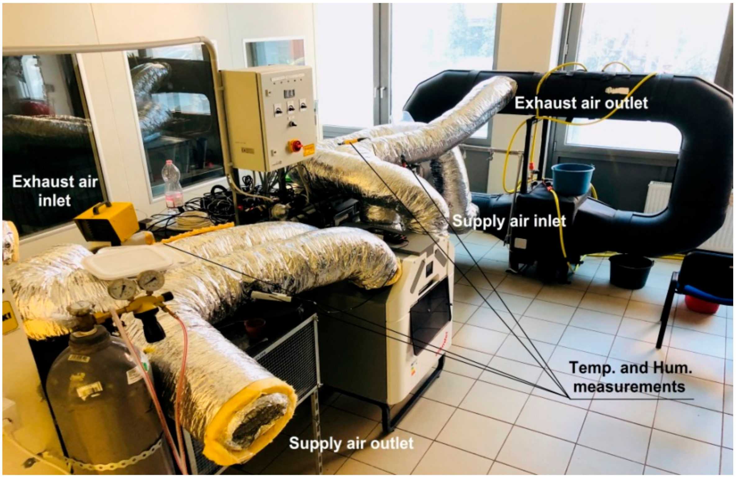
The effectiveness of a polystyrene material-based counter-flow heat exchanger (PHE) and a polymer membrane (polyethylene–polyether copolymer) material-based counter-flow energy exchanger (PEE) integrated in a Zehnder ComfoAir 350 ventilation device was investigated experimentally (Figure 1) under steady-state conditions. These exchangers are basically counter-flow types, but their inlet sections are from cross-flow zones as thermally and energy wasteful corners. The remaining cross-flow zones do not play as crucial a role if the counter-flow zone has sufficient surface area. For the cross-flow zones, the plates are employed; otherwise, the stream-joining problem would once again arise. For the counter-flow zones, it is possible, so as to increase efficiency, to subdivide the plates and make use of ducts (Table 1). This results in more surface area being available for heat and moisture exchange.
The height of the duct is very small (2.5 to 4 mm), allowing a very large exchange area to be packed into a small volume [21].
An additional objective was to be able to carry out the measurements within the widest possible range.
2.1.1. Setting of Air Temperature of Fresh Air (Supply Air Inlet)
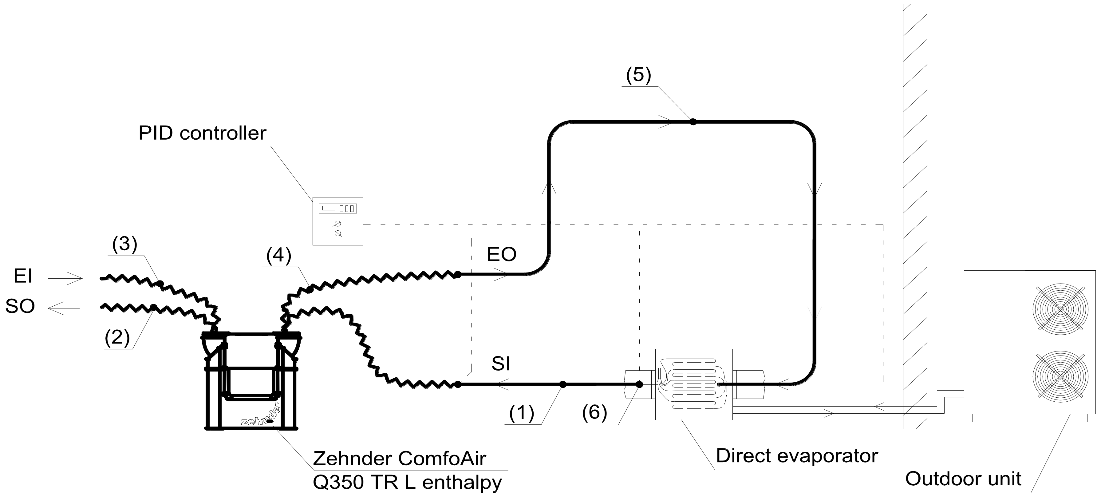
The target value of supply inlet air temperature (tsi (°C)) was set by an SCMI-01 proportional–integral–derivative (PID) controller unit (Figure 2).
Considering the set supply air inlet temperature and based on the measured actual supply air inlet temperature and surface temperature of the direct evaporator, the PID controls the necessary performance of the compressor through the continuous modification of the direct current (DC) inverter speed control regulation.
2.1.2. Setting of Air Humidity of Fresh Air (Supply Air Inlet Section)
The relative humidity of the supply air inlet section (RHsi (%)) was set by water atomizers placed at point (5) in Figure 2. The material of these atomizers was ceramic, supplied from the tap water. The required mass flow of the water medium was regulated by Herz radiator valves.
2.1.3. Air Temperature and Humidity Settings on Exhaust Air Inlet Section
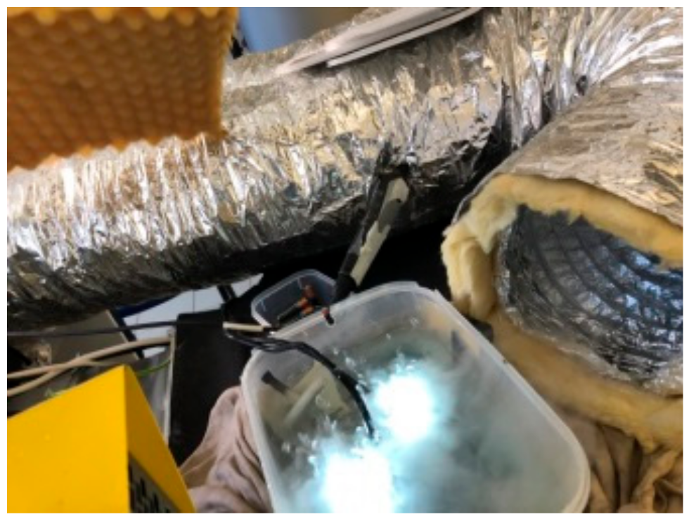
To provide a constant exhaust air inlet temperature (tei (°C)), a HOME FK 30 electrical heater and, to keep constant relative humidity (RHei (%)), ultrasonic humidifiers were placed close to the incoming exhaust air into the test facility (Figure 3).
2.1.4. Experimental Data Recording and Evaluation
Temperature and relative humidity data were recorded using a TESTO480 data recorder with TESTO sensors, placed into the middle of the air ducts at measurement points (1), (2), and (3) indicated in Figure 2. The set air volumetric flow rates were controlled by a TESTO Smartprobes 405i hot-wire anemometer. The values of the effectiveness were determined from the conducted measured values using Equation (1) [20,22].
where “T” as the temperature in °C is substituted in the case of sensible effectiveness, “x” as the humidity ratio in kg/kg is substituted in the case of latent effectiveness, and “h” as enthalpy in kJ/kg is substituted in the case of total effectiveness in place of “X” in Equation (1); therefore, ε is indexed as εs in the case of sensible effectiveness, εl for latent effectiveness, and εT for total effectiveness. The test conditions were significantly extended for the supply air inlet condition parameters (ambient temperature, humidity, enthalpy) compared with the existing standard (EN 13141-7) used in this research work.
2.2. Description of the Test Plan
The measurement plan was compiled on the basis of the following aspects:
- The test plan was basically divided into two ambient air conditions (winter outdoor air conditions for heating performance tests and summer outdoor air conditions for cooling performance tests).
- Based on Table 2, the extract air inlet relative humidity was set as 38% for heating performance tests and 47% for cooling performance tests during the experiments.
- A further objective was to perform tests in much wider outdoor air conditions than the EN 13141-7 standard instructs, extending also the values of effectiveness given by the producer. In this way, a 5 °C outdoor air temperature step change was managed in the range between −15 and 10 °C, and the outdoor air relative humidity was step-changed by 10% in the range between 70% and 100% for heating performance tests. For cooling performance tests, the outdoor air conditions were set between 27 and 40 °C with a 5 °C step change and between 40% and 90% with a 10% step change.
- The achievable humidity was in a ratio applicable to all states of operation, with equal distribution of achievable relative humidity.
- All tests were conducted under four different air volume flow rates (100, 200, 300, and 350 m3/h).
- The pressure difference between supply and exhaust fan was zero during the tests.
- The order of setting the steady-state test variables was the following before data recording: air volume flow rate, supply air inlet temperature, and finally the supply air inlet relative humidity.
- All tests were conducted under continuous monitoring of the supply air inlet relative humidity variables using the data collector instrument.
- The duration of each experimental test for every sequence order was at least 3000 s with a measurement rate of one per second to get the steady-state values. The sequence of measurements for all input parameters was conducted until the system reached the steady-state conditions.
3. Results and Discussion
The sensible, latent, and total effectiveness values of the polystyrene material-based counter-flow heat exchanger (PHE) and the polymer membrane (polyethylene–polyether copolymer) material-based counter-flow energy exchanger (PEE) are presented in this section, as calculated from the experimentally measured data for winter and summer tests. In addition, the sensible effectiveness of the PHE and PEE exchangers are compared under the same conditions.
3.1. Effectiveness of Air-to-Air PEE Energy Exchanger
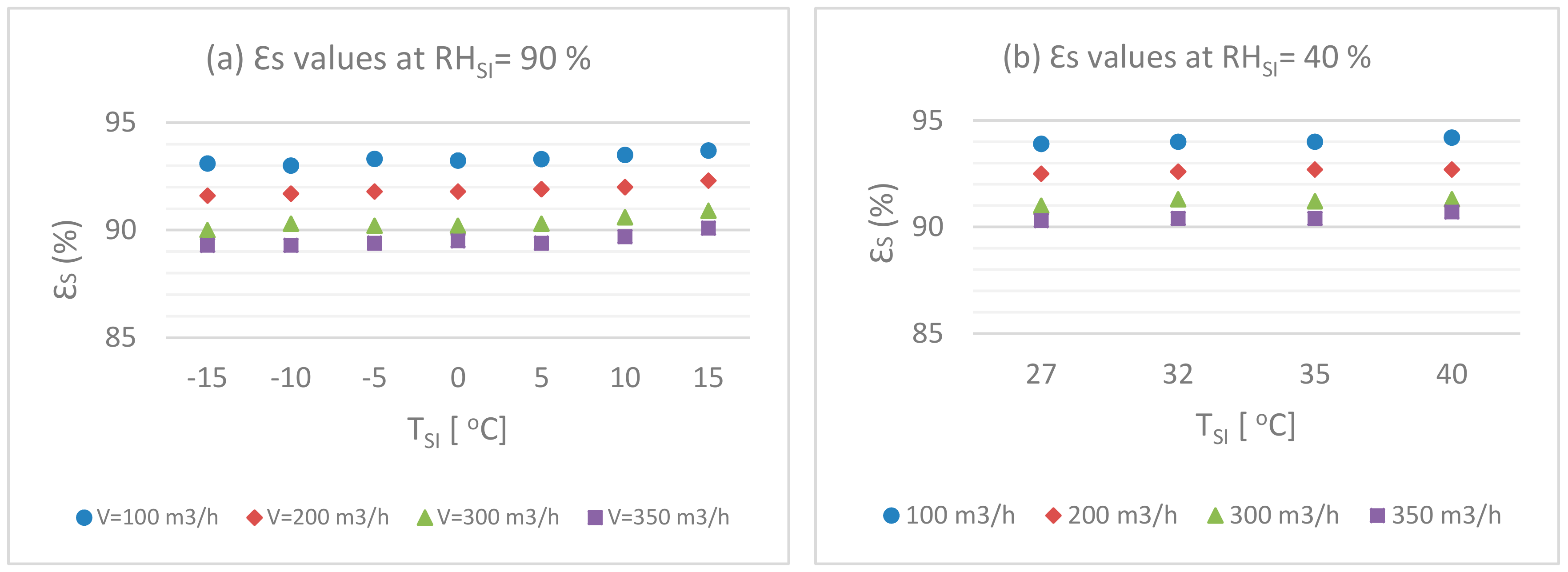
3.1.1. Sensible Effectiveness vs. Dry-Bulb Temperature of PEE
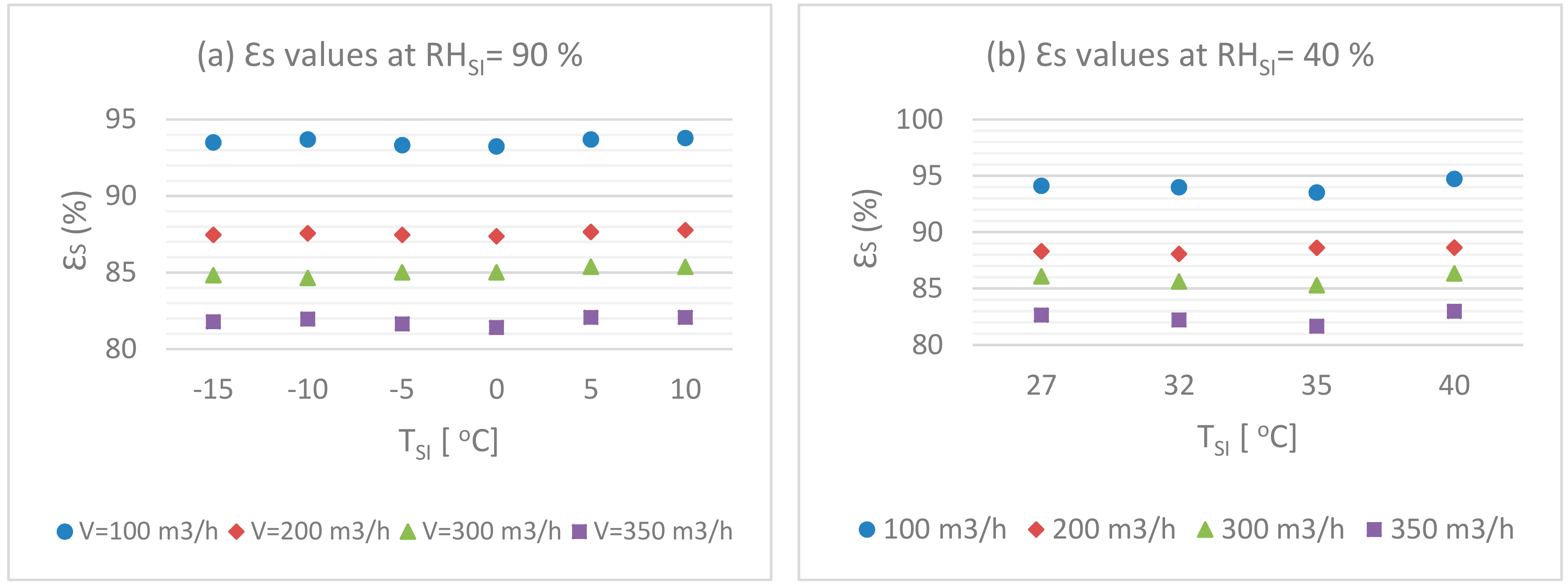
Figure 4 shows the sensible effectiveness vs. dry-bulb temperature at different volume flow rates for winter conditions (RH = 90%) and summer conditions (RH = 40%). It is noticeable that a slight increase in effectiveness occurs as the dry-bulb temperature increases. However, the trend for different volume flow rates shows that the highest effectiveness occurred at the lowest volume flow rate.
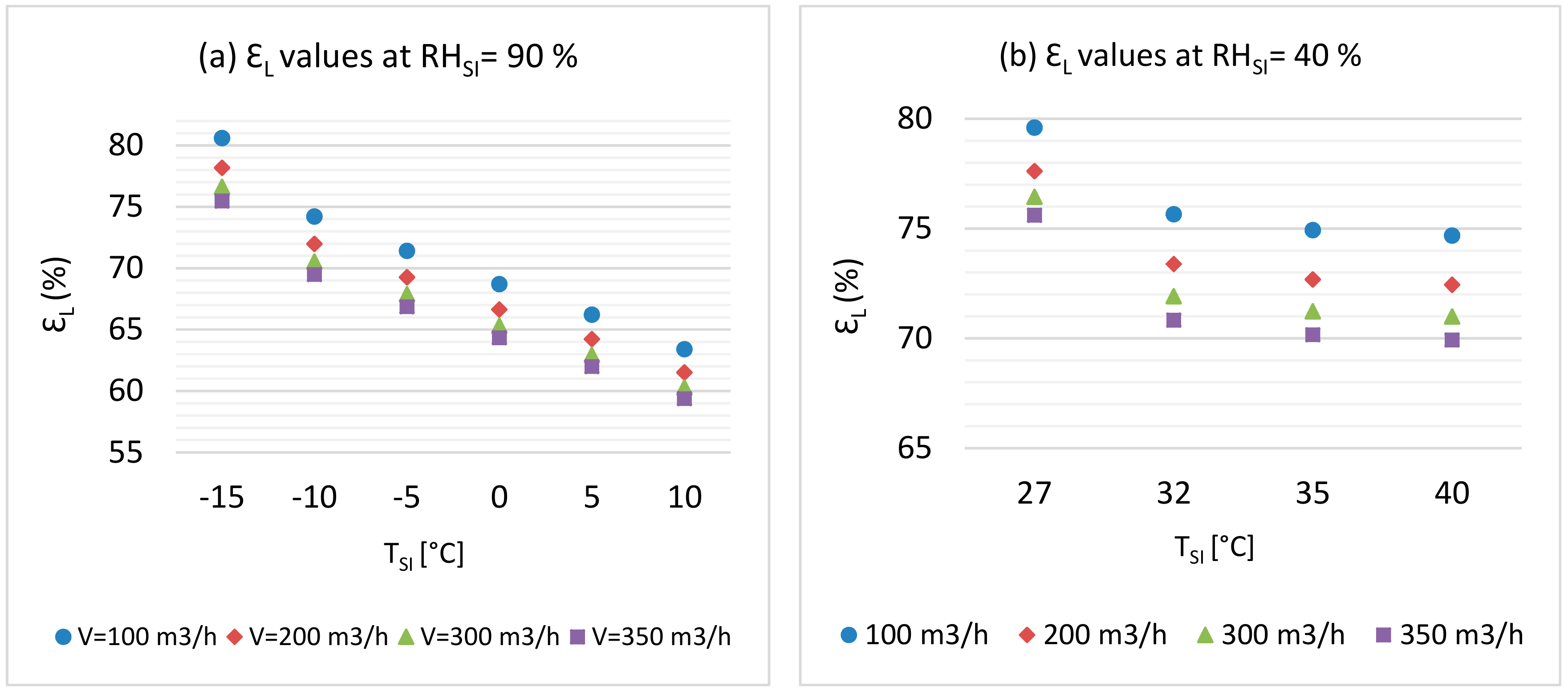
3.1.2. Latent Effectiveness vs. Dry-Bulb Temperature of PEE
Figure 5 shows the latent effectiveness vs. dry-bulb temperature at different volume flow rates for winter conditions (RH = 90%) and summer conditions (RH = 40%). It is clear that a decrease in effectiveness happened as the outdoor temperature increased in winter, and the trend shows a decreasing in effectiveness when the volume flow rate increases. On the other hand, the trend for different volume flow rates for the effectiveness in summer conditions shows that the highest effectiveness occurred at the lowest temperature, and the trend shows a major difference between the effectiveness at 27 °C and that at other temperatures.
Based on the results, the average values of latent effectiveness for the PEE were 69% in the winter and summer period.
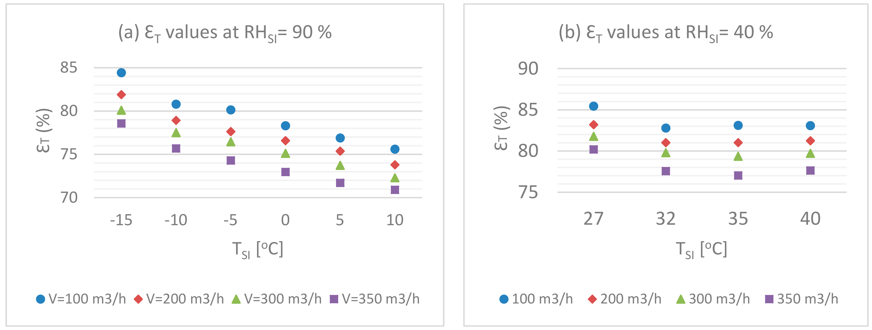
3.1.3. Total Effectiveness vs. Dry-Bulb Temperature of PEE
Figure 6 shows the total effectiveness vs. dry-bulb temperature at different volume flow rates for winter conditions (RH = 90%) and summer conditions (RH = 40%). It is obvious that there is a decrease in effectiveness while the outdoor temperature increases in winter conditions, and a decrease in effectiveness when the volume flow rate increases. On the other hand, the highest effectiveness occurred at the lowest temperature in summer conditions.
Based on the results, the average values of total effectiveness of the PEE were 77% in the winter and 78% in the summer.
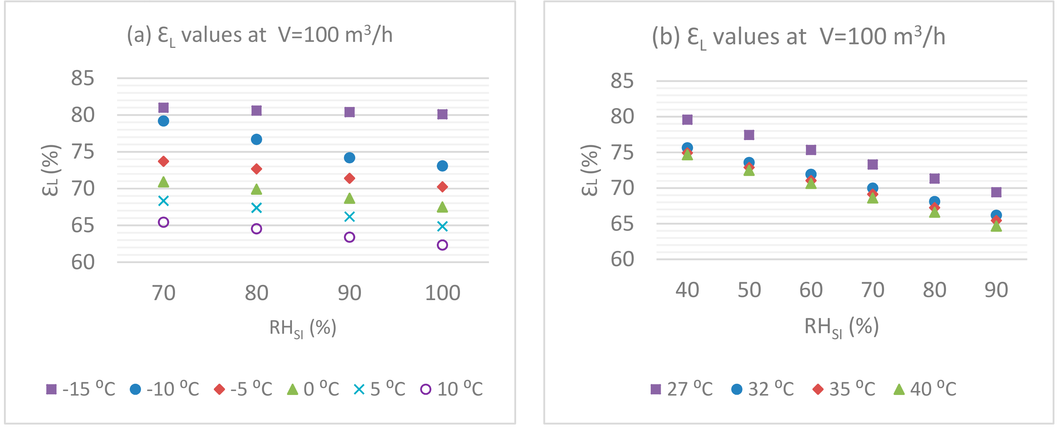
3.1.4. Latent Effectiveness vs. Relative Humidity of PEE
The correlation of latent effectiveness and relative humidity at a volume flow rate = 100 m3/h for winter conditions and for summer conditions is presented in Figure 7. It can be seen that there is a slight decrease in effectiveness when the relative humidity increases in winter conditions, while, in summer conditions, the decrease in effectiveness is more obvious. On the other hand, the trend for different temperatures in terms of the effectiveness shows that the effectiveness decreases when the dry-bulb temperature decreases.
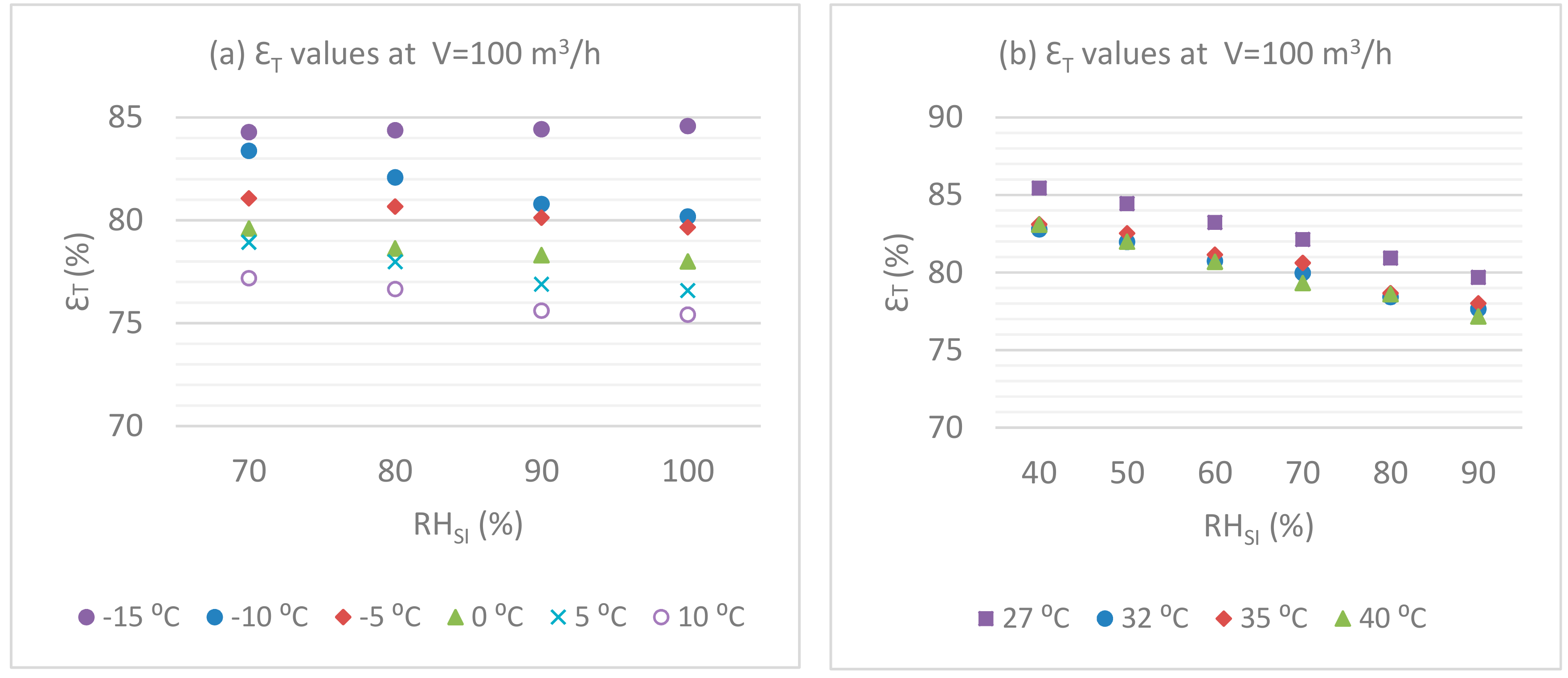
3.1.5. Total Effectiveness vs. Relative Humidity of PEE
The correlation of total effectiveness and relative humidity at a volume flow rate = 100 m3/h for winter conditions and for summer conditions is presented in Figure 8. Here, it can be seen that effectiveness decreases when the relative humidity increases. In addition, the effectiveness trend for different dry-bulb temperatures decreases when the temperature increases.
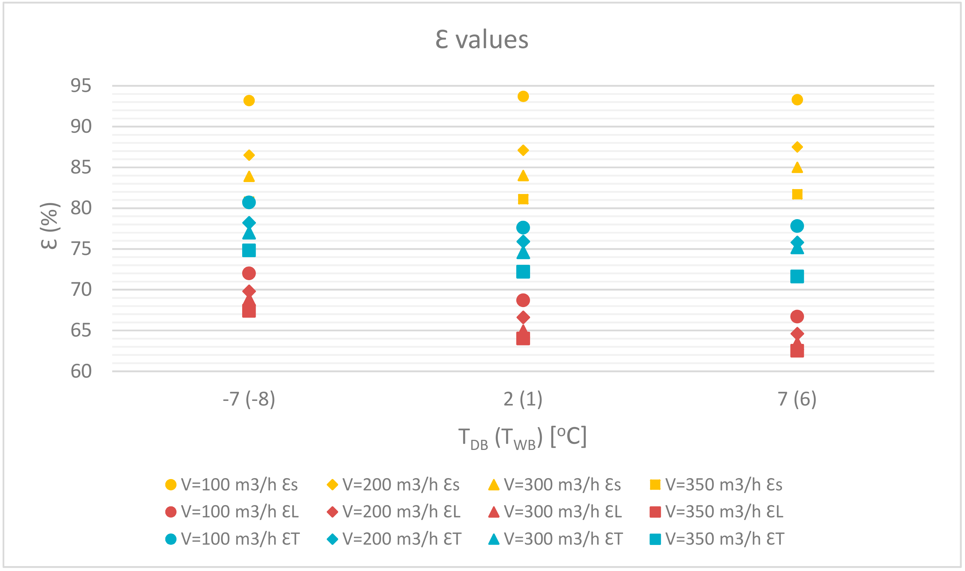
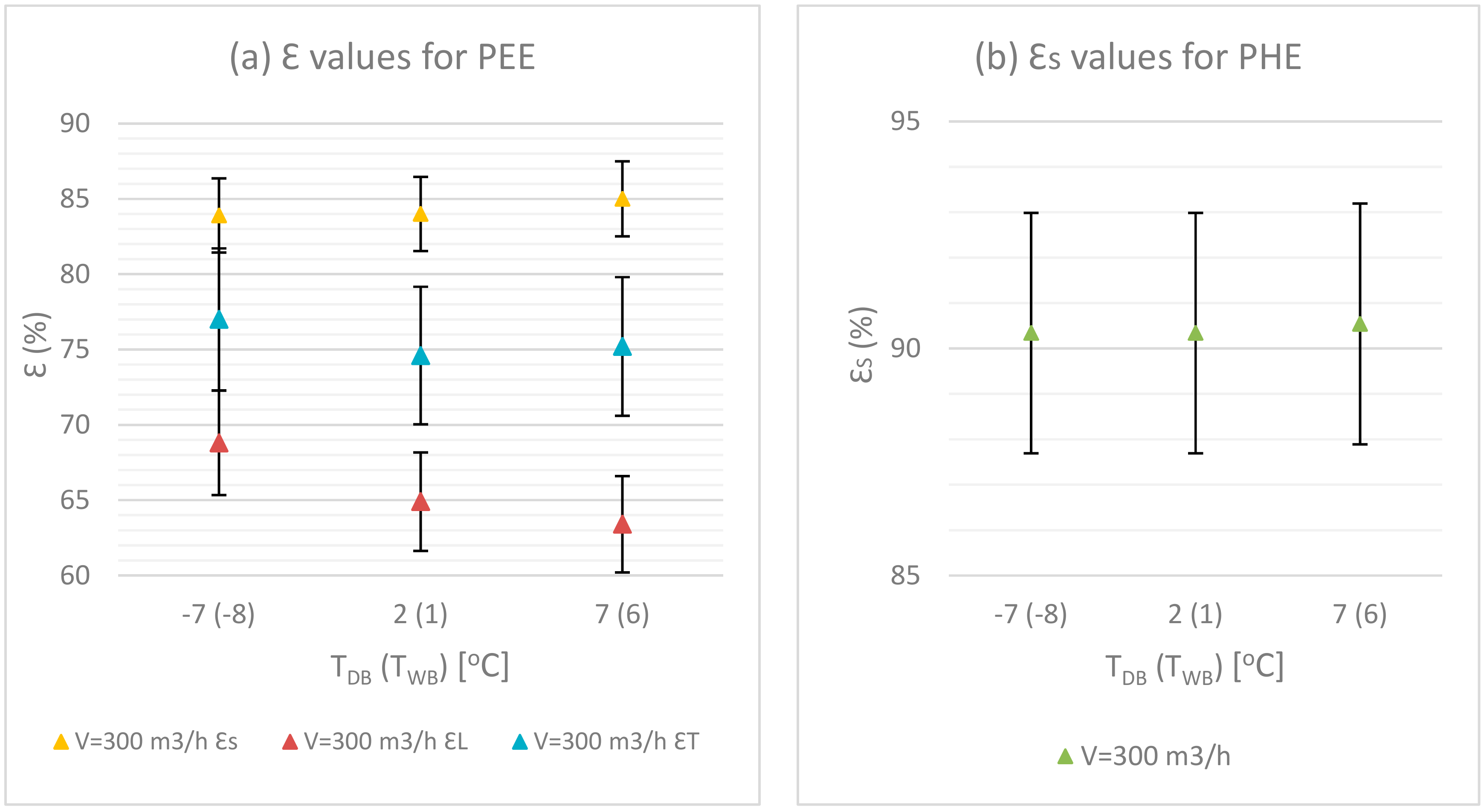
3.1.6. Effectiveness vs. Outdoor Air Inlet Dry Temperature for EN Standards
The experimental test of heating performance (winter conditions) was taken in accordance with outdoor temperature conditions defined in EN standards. It was measured separately for winter conditions, unlike the cooling performance (summer conditions), which was included in the summer conditions test plan. Figure 9 below illustrates all the effectiveness values vs. dry-bulb (wet-bulb) temperatures as defined in EN standards.
3.2. Effectiveness of Air-to-Air PHE Heat Exchanger
3.2.1. Sensible Effectiveness vs. Dry-Bulb Temperature of PHE
Figure 10 shows the sensible effectiveness vs. dry-bulb temperature at different volume flow rates for winter conditions (RH = 90%) and summer conditions (RH = 40%). It is clearly that a slight increase in effectiveness occurs when the dry-bulb temperature increases. However, the highest effectiveness occurred at the lowest volume flow rate.
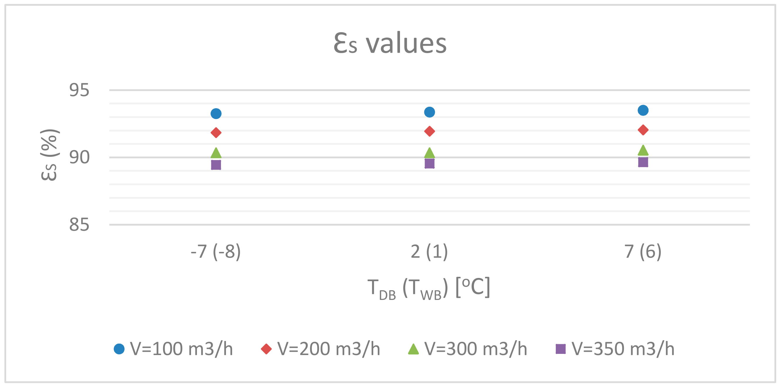
3.2.2. Sensible Effectiveness vs. Outdoor Air Inlet Dry Temperature for EN Standards
Figure 11 shows the correlation of sensible effectiveness and outdoor air inlet temperature as defined in EN standards under different volume flow rates. It can be seen that a slight increase in effectiveness occurs as the dry-bulb temperature increases.
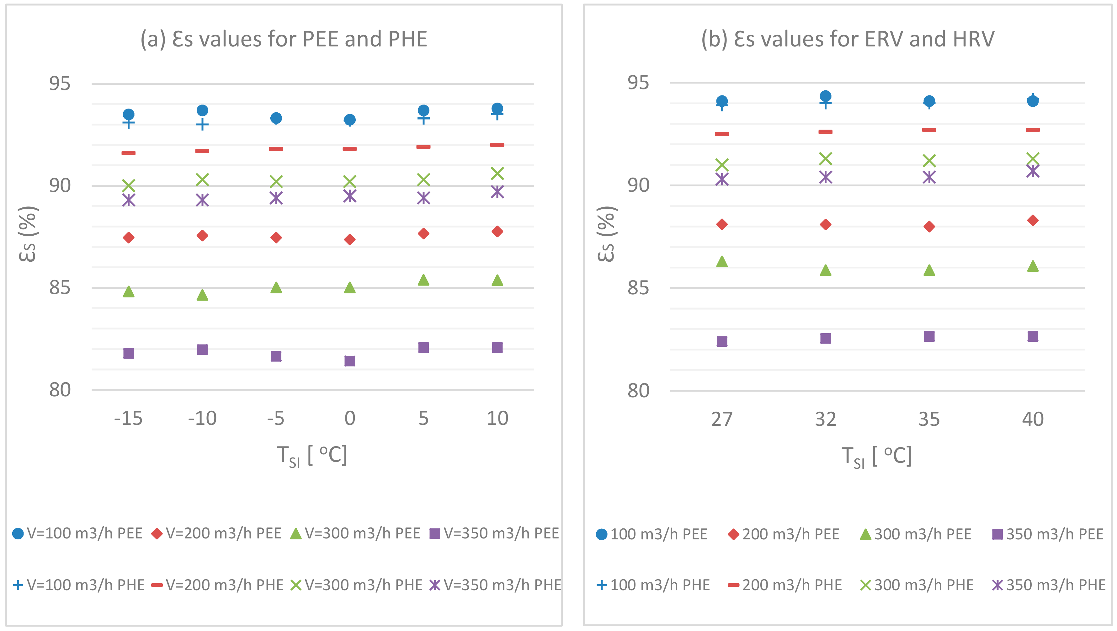
3.2.3. Sensible Effectiveness Comparison between the PEE and PHE Exchangers
Figure 12 shows the comparison of sensible effectiveness of PEE and PHE exchangers under different dry-bulb temperatures and different volume flow rates for winter and summer conditions. The results show that the PHE overall has higher sensible effectiveness than the PEE, especially at higher air volume flow rates. Based on the results given by the tests, the average sensible effectiveness values for PHE in winter and summer conditions were 91% and 92% respectively, while the average sensible effectiveness values for PEE were 87.2% in winter conditions and 87.8% in summer conditions.
The maximum values of sensible effectiveness were recorded in summer test conditions (with 40 °C ambient air as the supply air inlet temperature), at an air volume flow rate of 100 m3/h, which were 94.2% for PHE and 94.1% for PEE.
3.3. Uncertainty Calculations
The uncertainties in calculations are discussed in this section in order to determine the percentage error while measuring. As in the most relevant research studies carried out in the field, following experimental tests, instead of statistical calculations [23], uncertainty calculations were performed. The discussion of the uncertainties in values of the energy performance of air-to-air heat and energy exchangers has higher practical implications in the field of building energy [19,24]. The uncertainty in the experiment can be divided into two types [25] as follows:
- Random uncertainty: instrument accuracy;
- Systematic uncertainty: measurement calibration.
It can be realized from the previous diagrams (Figure 4, Figure 5, Figure 6, Figure 7, Figure 8, Figure 9, Figure 10, Figure 11 and Figure 12) in this paper that there were fluctuations in the values of effectiveness. The reason for these fluctuations is probably due to a release of water from the water atomizers that sprinkle water into the supply inlet air. In addition, the steam from ultrasonic humidifiers in the exhaust inlet air causes a delay, and fluctuations were also observed while using the TESTO hot-wire anemometer. With these changes in temperature and moisture conditions, irregularities may have occurred in calculating the values of effectiveness.
The random uncertainty was calculated using the Kline and McClintock method [25] for estimating uncertainty in experimental results.
The basic principle of the Kline and McClintock method [25] is explained in Appendix A.
The systematic uncertainty was given by the manufacturers of the measurement devices. Table 3 below represents the calibration and the uncertainty for the TESTO hot-wire anemometer.
Below, we took one sample to evaluate the following parameters in order to calculate the uncertainty in the effectiveness:
- 1
- Volumetric flow rate = 300 m3/h;
- 2
- Temperature of the supply air inlet = −7 °C;
- 3
- Relative humidity of the supply air inlet = 75%;
- 4
- Temperature of the exhaust air inlet = 20 °C;
- 5
- Relative humidity of the exhaust air inlet = 38%.
Uncertainty in sensible effectiveness was calculated using Equations (3)–(6) as follows:
Uncertainty in latent effectiveness was calculated using Equations (7)–(10) as follows:
Uncertainty in total effectiveness was calculated using Equations (11)–(14) as follows:
Figure 13 demonstrates the uncertainties for all values of effectiveness as a function of dry-bulb ambient temperature for PEE and PHE at an air volume flow rate of 300 m3/h for heating performance tests based on EN standards.
3.4. Energy Calculations
This section introduces the effects of the material of the two investigated exchangers on the energy consumption of ventilation in three different EU climates (in Reykjavík in Iceland as a cold climate, in Budapest in Hungary as a temperate climate, and in Rome in Italy as a warm climate). To achieve this, seasonal average data for effectiveness (Table 4) were determined based on the conducted test results. The energy calculations were performed with an air volume flow rate of 300 m3/h and an air density constant of 1.2 kg/m3.
3.4.1. Utilization of Test Data for Energy Calculations
The meteorological data for each investigated EU city were generated by the TRNSYS 18 transient system simulation tool using the Meteonorm database in an hourly period. To perform energy calculations, ambient temperature duration curves were used for PHE. In the case of PEE, the usage of the ambient enthalpy duration curve for energy calculations is inappropriate, because there is a range for enthalpy at a given temperature based on the psychometric chart. To achieve the energy estimations for PEE, ambient temperature–enthalpy graphs were used. The frosting starts appearing when the ambient temperature is lower than the frosting temperature (−5 °C for PEE and 0 °C for PHE, based on the technical information given by the producer). An electrical pre-heater was assumed for the energy calculations, and the exhaust inlet conditions (constant 20 °C exhaust air inlet dry-bulb and 12 °C wet-bulb temperature) were considered based on the EN 13141-7 standard; there was no decreasing effect of frosting on the effectiveness of the exchangers in the heating period. During the energy calculations, the bypass activation was also neglected, which reduces or shuts off recovery when it is not needed under transient weather conditions in reality.
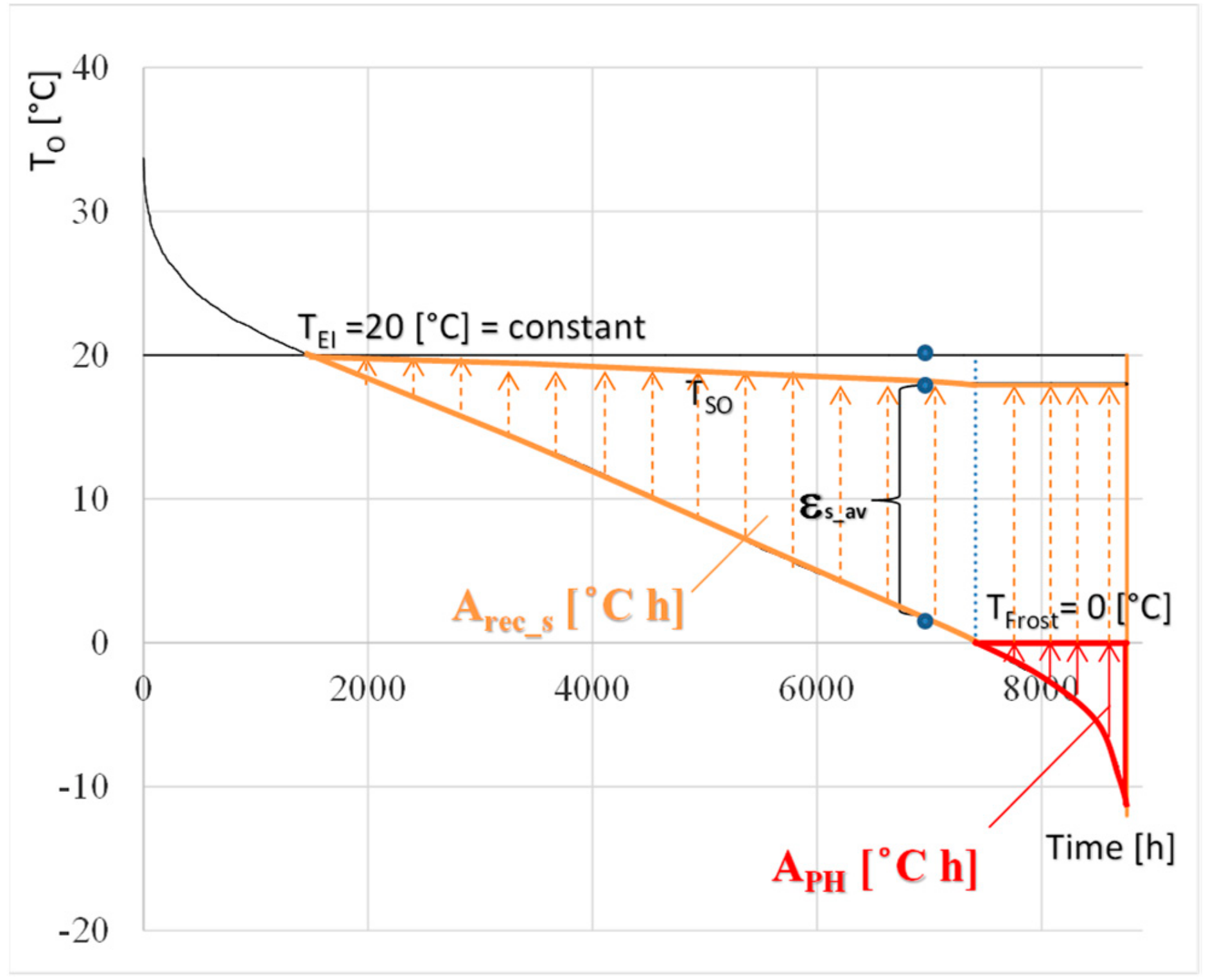
For sensible heat recovery calculations using the sensible average data for effectiveness from the tests (Table 4), the air temperature (Tso) after the PHE could be calculated with Equation (15).
where Tso is the supply outlet air temperature in °C that is supplied into the conditioned space, To is the ambient air temperature in °C, TEI is the exhaust inlet air temperature in °C, and εs_av is the seasonal average data for sensible effectiveness.
Since the pre-heater heats up the ambient air to the frosting temperature, the frosting temperature (TFrost) was used in Equation (15) for values under the ambient air temperature (To).
In this way, the areas that represent the energy consumption of the pre-heater (APH) and ventilation sensible energy saved by heat recovering (Arec_s) were determined on the ambient temperature duration curve for the heating period (Figure 14). Considering the limitation of the paper and so as to avoid repetition, Budapest, the capital of Hungary, was selected to introduce the developed energy calculation procedure. Since Budapest is located in a temperate climate region in Europe, the city has wider weather conditions considering both colder winter and warmer summer seasons.
Using the defined areas, the sensible energy saved and energy consumption of the pre-heater could be calculated using Equations (16) and (17), respectively.
where cPair is the specific heat capacity of the air in kJ/kg∙°C, is the mass flow rate of the air in kg/h, ρair is the density of the air in kg/m3, is the air volume flow rate, Arec_s is the area proportional to the sensible heating energy recovery in h∙°C (Equation (18)), and APH is the area proportional to the pre-heater energy consumption in h∙°C (Equation (19)).
where τ is the time in h.
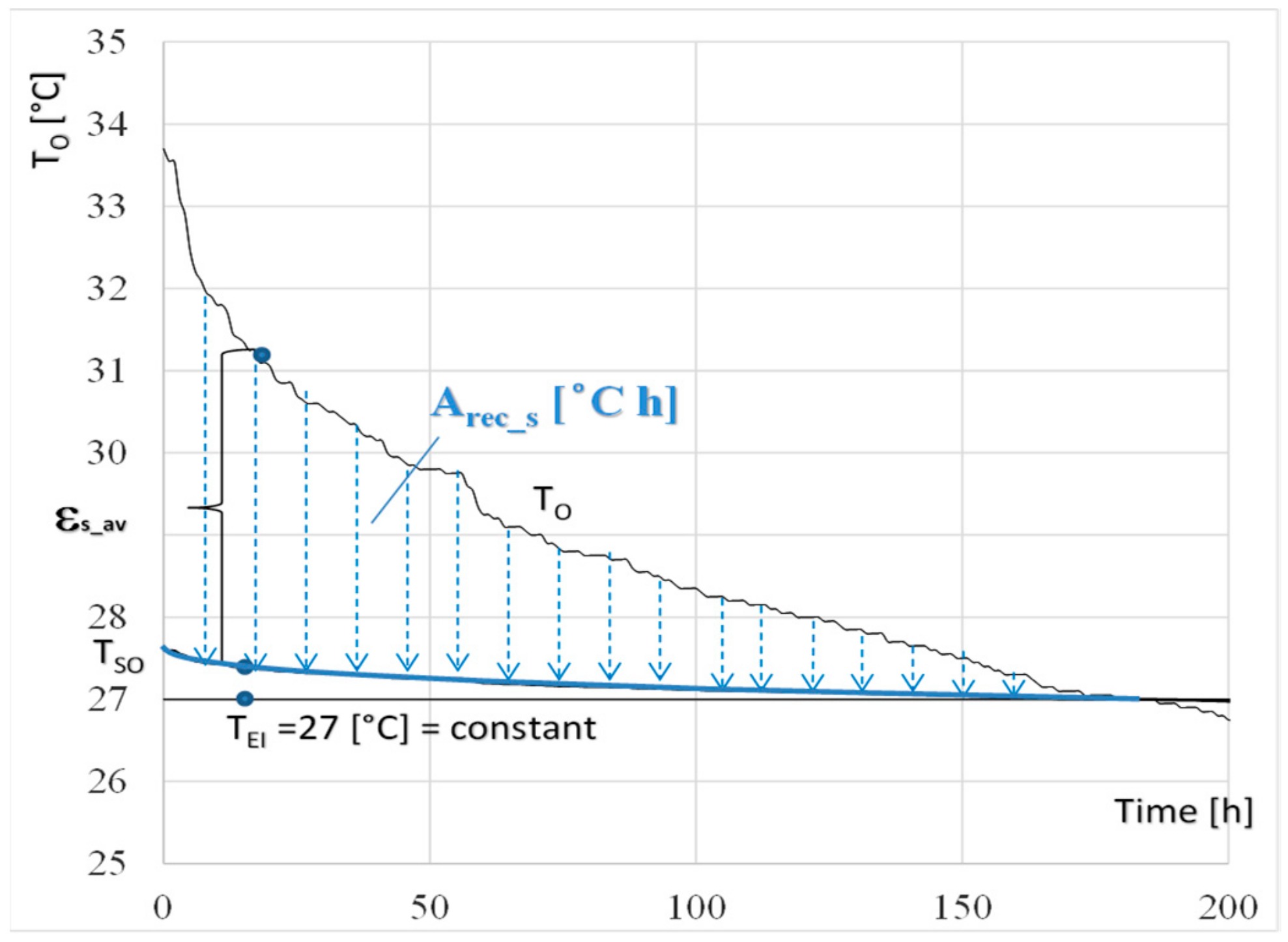
The area that represents ventilation sensible energy saved by heat recovery (Arec_s) can be seen on the ambient temperature duration curve (Figure 15) during the cooling period. Moreover, for the calculations, a 27 °C dry-bulb and 19 °C wet-bulb exhaust air inlet constant temperature (EN 13141-7) was assumed during the cooling period.
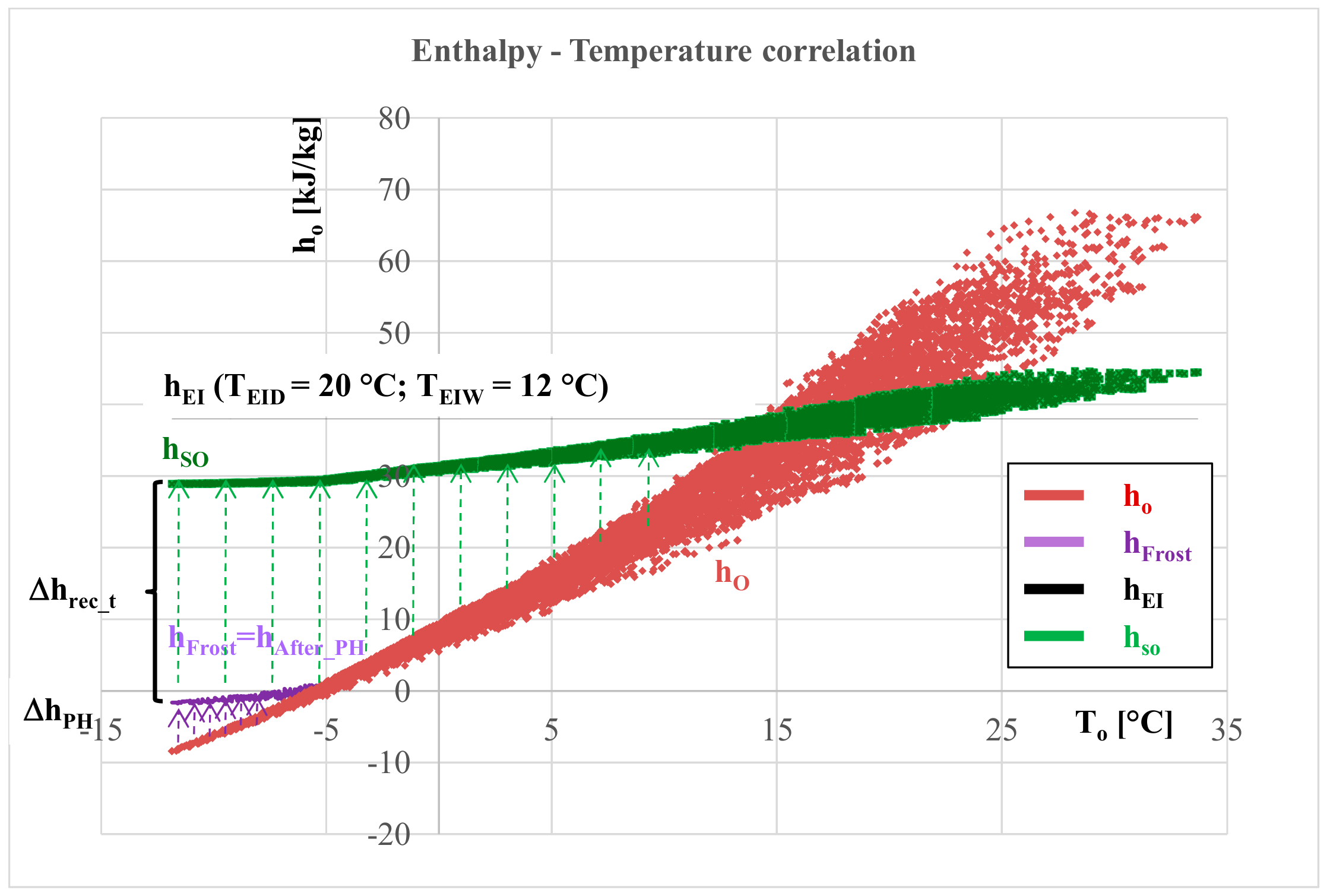
Using the seasonal average data for total effectiveness (Table 4) of the energy recovery, and assuming a given constant exhaust enthalpy value, the supply outlet air enthalpy (hso) after the PEE exchanger could be calculated with Equation (20).
where hso is the supply outlet air enthalpy in kJ/kg∙°C that is supplied into the conditioned space, ho is the ambient air enthalpy in kJ/kg∙°C, hEI is the exhaust inlet air enthalpy in kJ/kg∙°C, and εt_av is the seasonal average data for total effectiveness.
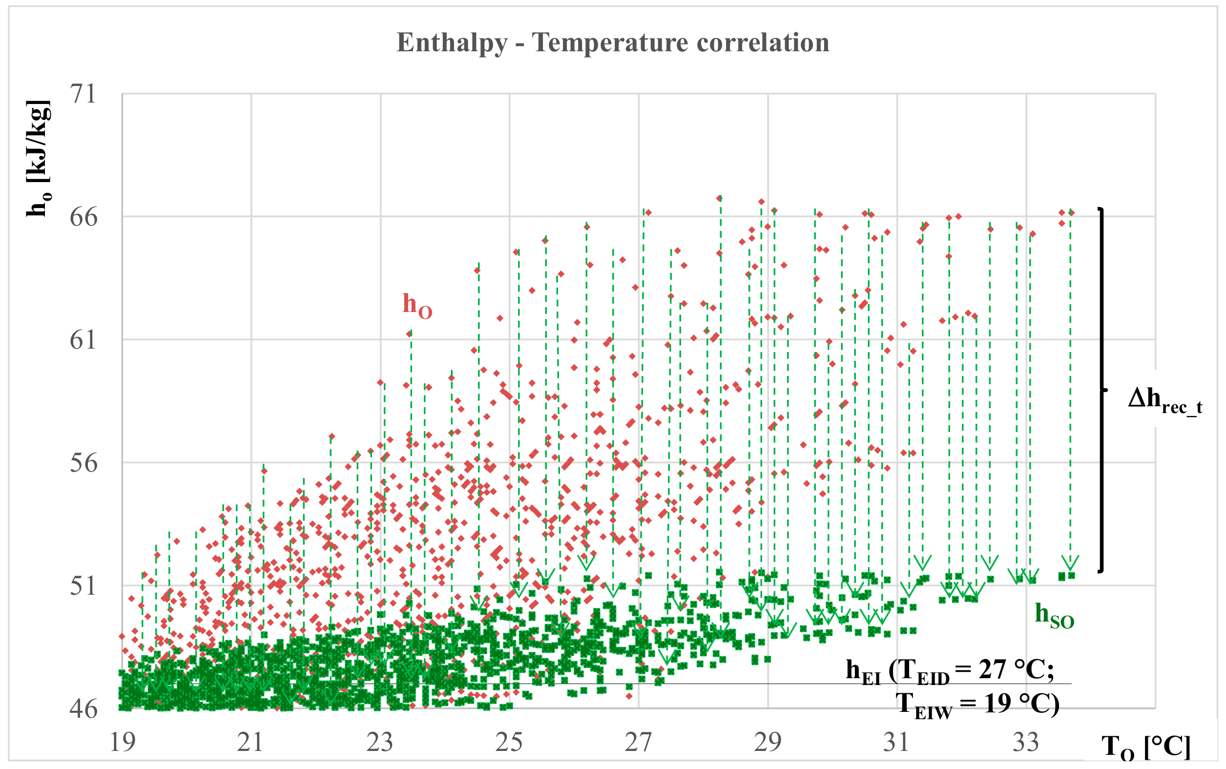
Since the pre-heater heats up the ambient air to the frosting enthalpy, the frosting enthalpy (hFrost) was used in Equations (20)–(21) for values under the ambient air enthalpy (ho). The areas that represent ventilation total energy saved by energy recovery (Arec_t) (Equation (21)) and the energy consumption of the pre-heater (APH) (Equation (22)) were determined on the ambient temperature-enthalpy graph during the heating period (Figure 16).
The area that represents the ventilation total energy saved by energy recovery (Arec_t) can be seen on the ambient temperature duration curve (Figure 17) during the cooling period.
3.4.2. Results of the Energy Estimation
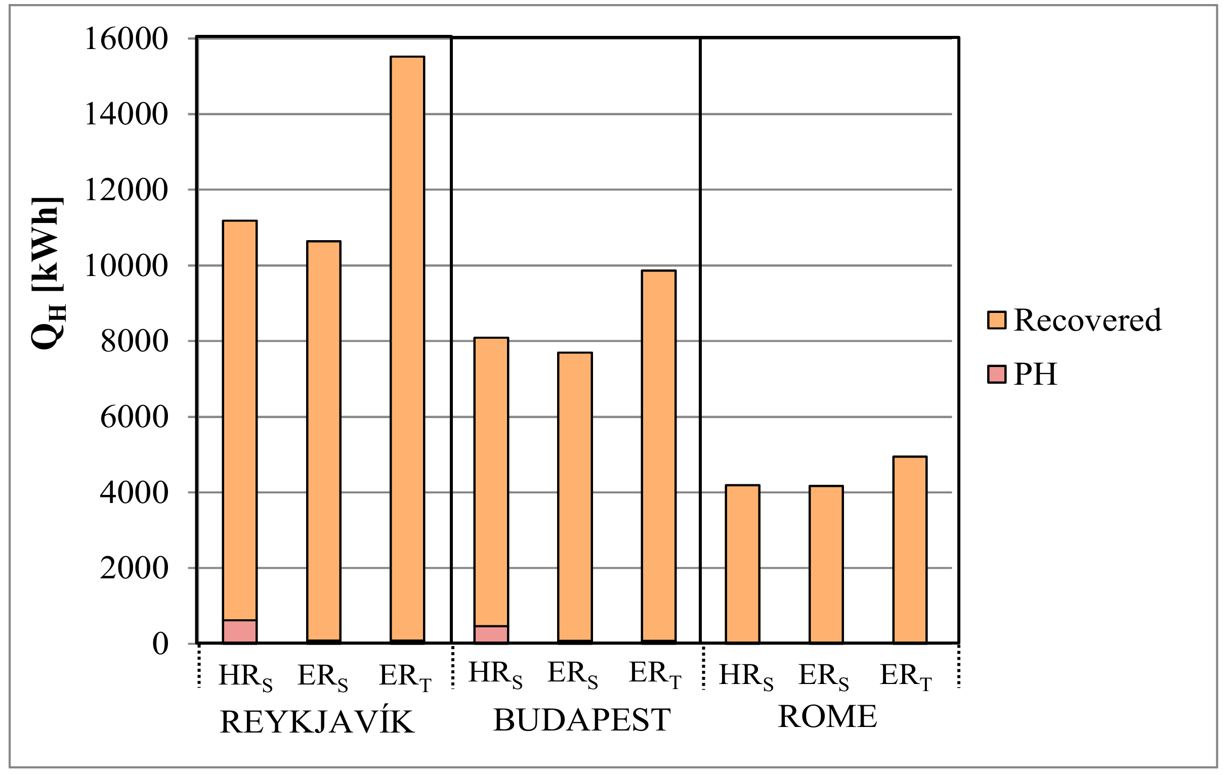
The calculated energy consumption of the pre-heater (PH), the ventilation sensible heat recovered by the PHE (HRS) and PEE (ERS), and the ventilation total energy recovered by the PEE (ERT) can be seen in Figure 18 during the heating period.
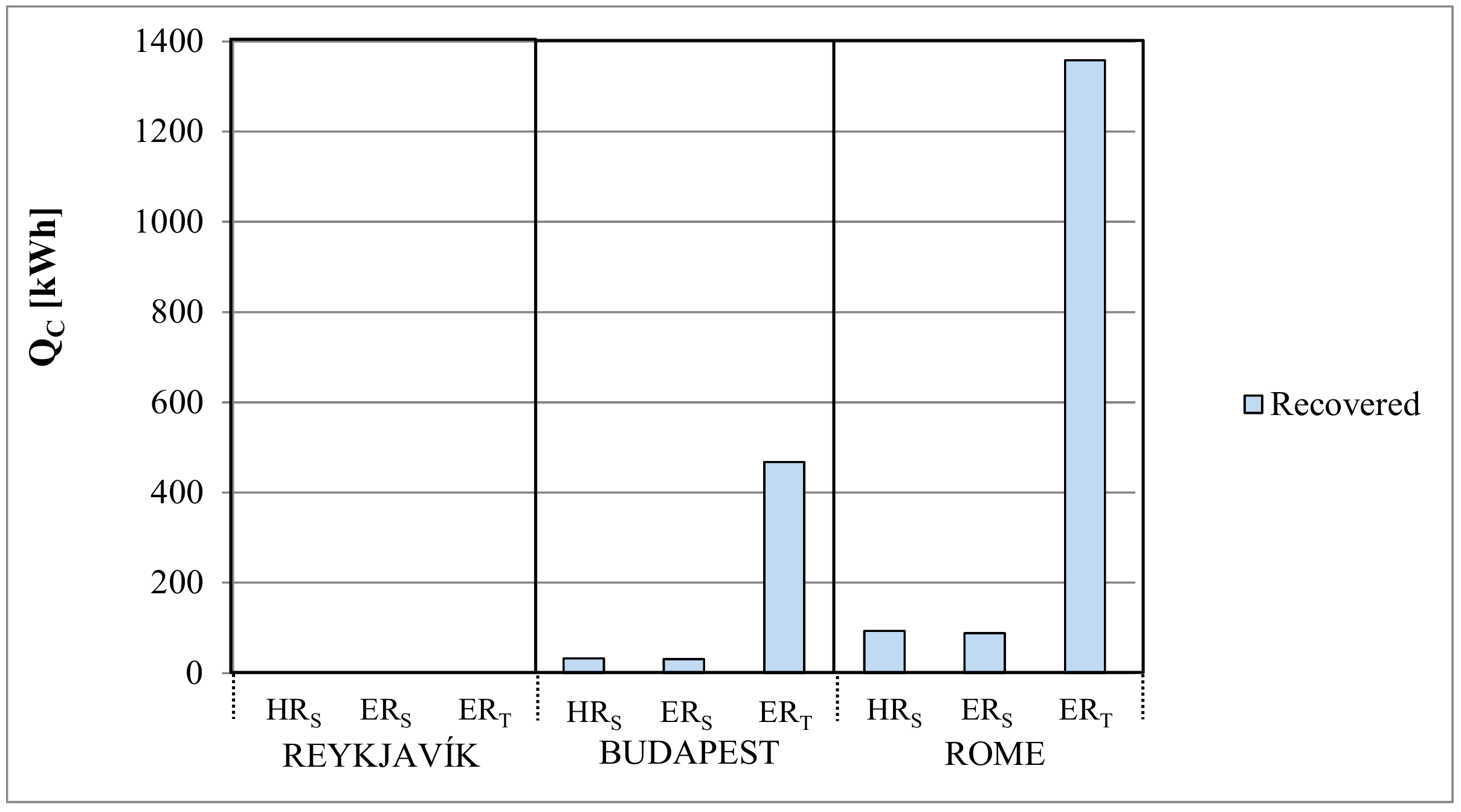
The calculated ventilation sensible heat recovered by the PHE (HRS) and PEE (ERS), and the ventilation total energy recovered by the PEE (ERT) can be seen in Figure 19 during the cooling period.
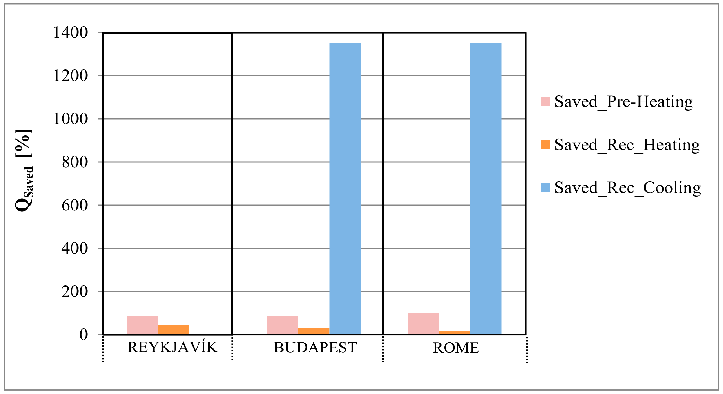
The difference in energy saved in terms of the pre-heating and ventilation energy recovered by the PEE and PHE was also calculated, showing the benefit of the PEE (Figure 20).
During our research work, experimental values for the effectiveness were used to calculate the annual ventilation energy saved by heat recovery with a polystyrene sensible air-to-air heat exchanger (PHE) and energy recovery with a polymer membrane air-to-air energy exchanger (PEE), along with the energy consumption of a pre-heater. The results are presented separately based on the exchanger material and different European climate regions: in Reykjavík in Iceland as a cold climate, in Budapest in Hungary as a temperate climate, and in Rome in Italy as a warm climate. During the energy investigation, temperature-controlled heat recovery and energy recovery was assumed. Based on the results, overall higher energy saving can be provided with the PEE than with the PHE operation. When using the PEE in the ventilation unit, the pre-heater consumes 87.1% in Reykjavík and 83.7% in Budapest, which is less energy than the PHE application, while, in Rome, the PEE does not require a pre-heater. When operating the ventilation unit with the PEE exchanger, the energy saving on the ventilation air is 46.04% higher in Reykjavík (as a cold climate), 28.46% higher in Budapest (as a temperate climate), and 18.09% higher in Rome (as a warm climate) during the heating period, and 1351.97% higher in Budapest and 1350.29% higher in Rome during the cooling period compared to the PHE, based on this study.
4. Conclusions
The objective of this research study was to investigate the sensible, latent, and total effectiveness values of a polystyrene material-based counter-flow heat exchanger (PHE) and a polymer membrane (polyethylene–polyether copolymer) material-based counter-flow energy exchanger (PEE) under several operating and ambient parameters that affect the effectiveness of the exchangers. Moreover, the effects of the material of both exchangers (polystyrene for the sensible heat exchanger and polymer membrane for the energy exchanger) on energy consumption of ventilation in European cities with three different climates (in Reykjavík in Iceland as a cold climate, in Budapest in Hungary as a temperate climate, and in Rome in Italy as a warm climate) were evaluated. The major findings obtained from this research work are summarized as follows:
- The results showed that the values of the sensible effectiveness under different outdoor air temperature and relative humidity values are almost the same values for the PEE and PHE, and only the air volume flow rate, as an operation parameter, has an effect on the sensible effectiveness.
- The maximum value of sensible effectiveness was found at the lowest air volume flow rate (100 m3/h), which was 94.2% for the PHE and 94.1% for the PEE in summer conditions. The reason for this much lower sensible effectiveness at higher air volume flow rates for the PEE is due to the transfer of additional moisture to the supply air stream from the exhaust air stream.
- The PEE is likely to be used when there is a need to maintain the indoor air relative humidity level during the winter heating period or to reduce the moisture of the outdoor air (as supply inlet air) during the summer cooling period.
- The values of the latent and total effectiveness decrease when the relative humidity of the outdoor air increases.
- The maximum values of the latent and total effectiveness could be obtained for the lowest outdoor air dry-bulb temperature values.
The results of the experiments showed that the values of the effectiveness of air-to-air counter-flow exchangers are higher than the cross-flow exchangers found in the literature [13,26,27].
The results of the experimental tests indicate the performance of the PEE and PHE. Concisely, it shows the optimal operating parameters from the point of view of energy saving. Based on the results, it is obvious that, if the indoor air quality requirements are lower, then using a polystyrene sensible air-to-air counter-flow heat exchanger (PHE) is suitable for heat recovery, and the investment cost is lower. If the total energy exchange (heat and moisture exchange for better indoor air quality) is important, then using the polymer membrane air-to-air counter-flow energy exchanger (PEE) is required. From the results, it is proven that the PEE exchanger performs better than the PHE in the investigated cold, temperate, and warm climate regions during operation for a whole year including heating and cooling periods. Even though the investment cost of PEE is higher, the amount of energy saved on the pre-heater can be 87.1% higher than when operating the ventilation unit with the PHE exchanger, based on this study.
Author Contributions
M.K. provided funding for the research and developed the test facility; L.A.-H. conducted the tests in the laboratory. The results and the analysis were performed by M.K. and L.A.-H. The text was written by M.K. and L.A.-H., and checked and amended by M.K.
Funding
This research project was financially supported by Zehnder Group Netherlands, Zehnder Group Deutschland GmbH, Hungarian Trade Representation, the National Research, Development, and Innovation Office from NRDI Fund [grant number: NKFIH PD_18 127907], and the János Bolyai Research Scholarship of the Hungarian Academy of Sciences, Budapest, Hungary. Moreover, the research reported in this paper was supported by the Higher Education Excellence Program of the Ministry of Human Capacities in the frame of the biotechnology research area of Budapest University of Technology and Economics (BME FIKP-BIO).
Acknowledgments
The authors wish to thank István Tóth and Tamás Bakó for providing the Zehnder ComfoAir 350 device for this research.
Conflicts of Interest
The authors declare no conflict of interest.
Abbreviations
| EI | Exhaust air inlet |
| EPBD | Energy Performance of Building Directive |
| h | Enthalpy (kJ/kg) |
| HVAC | Heating, ventilation, and air-conditioning |
| Air mass flow rate (kg/h) | |
| NZEB | Nearly zero-energy buildings |
| O | Outdoor |
| PEE | Polyethylene–polyether copolymer material-based counter-flow air-to-air energy exchanger |
| PHE | Polystyrene material-based counter-flow air-to-air heat exchanger |
| RH | Relative humidity (%) |
| T | Temperature (°C) |
| Air volume flow rate (m3/h) | |
| x | Absolute humidity (gwater/kgdry air) |
| Greek Letters | |
| εs | Sensible effectiveness |
| εL | Latent effectiveness |
| εT | Total effectiveness |
| ωR | Random uncertainty |
| τ | time (h) |
| Subscripts | |
| EI | Exhaust air inlet |
| O | Outdoor |
| SI | Supply air inlet |
| SO | Supply air outlet |
Appendix A
Kline and McClintock established a method to calculate the uncertainty. They defined the uncertainty as a range where the true value lies in the mean ± uncertainty interval (b to 1).
For example, if a temperature measurement was as follows (Equation (A1)):
then the ± sign in Equation (A1) means that the experimenter is not sure about the results, and it defines the range where the true value lies. In the example above, the experimenter implies that the true value lies between 24 °C and 26 °C.
T = 25 °C ± 1 °C,
As an explanation of how these uncertainties propagate into the results, let the result R be a function of an independent number (n) of variables ,, …., (Equation (A2)):
For a small variation in the variables, this relationship can be expressed in linear form as follows (Equation (A3)):
Based on the first theorem defined by Kline and McClintock, if R is a linear function of n independent variables, and if the maximum deviation of the ith variable from its mean is , then the maximum deviation of R from its mean value is given by Equation (A4).
Equation (A4) might be used as an approximation for calculating the uncertainty interval in the result by simply substituting for as follows:
Equation (A5) can be referred to as the linear equation. Based on the second theorem defined by Kline and McClintock, if R is a linear function of n independent variables, each of which is distributed with a standard deviation , then the standard deviation of R is given by Equation (A6).
The best measure of uncertainty is neither the maximum value nor the standard deviation, but some interval based on certain odds. For the special case in which the variables are distributed normally, the distribution of the results will also be normal, and the third theorem described below applies. Based on the third theorem defined by Kline and McClintock, if R is a linear function of n independent variables, each of which is normally distributed, then the relationship between the interval for the variables and the interval for the results , which gives the same odds for each of the variables and for the results, is given by Equation (A7).
Equation (A7) is used directly as an approximation for calculating the uncertainty interval in the result. It is referred to as the second-power equation.
References
- Ferrara, M.; Monetti, V.; Fabrizio, E. Cost-optimal analysis for nearly zero energy buildings design and optimization: A critical review. Energies 2018, 11, 1478. [Google Scholar] [CrossRef]
- Tsirigoti, D.; Tsikaloudaki, K. The effect of climate conditions on the relation between energy efficiency and urban form. Energies 2018, 11, 582. [Google Scholar] [CrossRef]
- Wan, K.K.W.; Li, D.H.W.; Liu, D.; Lam, J.C. Future trends of building heating and cooling loads and energy consumption in different climates. Build. Environ. 2011, 46, 223–234. [Google Scholar] [CrossRef]
- Sailor, D.J.; Pavlova, A.A. Air conditioning market saturation and long-term response of residential cooling energy demand to climate change. Energy 2003, 28, 941–951. [Google Scholar] [CrossRef]
- Lam, J.C.; Tang, H.L.; Li, D.H.W. Seasonal variations in residential and commercial sector electricity consumption in Hong Kong. Energy 2008, 33, 513–523. [Google Scholar] [CrossRef]
- Giannakopoulos, C.; Hadjinicolaou, P.; Zerefos, C.; Demosthenous, G. Changing energy requirements in the Mediterranean under changing cimatic conditions. Energies 2009, 2, 805–815. [Google Scholar] [CrossRef]
- Karlsson, J.; Roos, A.; Karlsson, B. Building and climate influence on the balance temperature of buildings. Build. Environ. 2003, 38, 75–81. [Google Scholar] [CrossRef]
- Calise, F.; D’Accadia, D.M.; Barletta, C.; Battaglia, V.; Pfeifer, A.; Duic, N. Detailed modelling of the deep decarbonisation scenarios with demand response technologies in the heating and cooling sector: A case study for Italy. Energies 2017, 10, 1535. [Google Scholar] [CrossRef]
- Ahmed, K.; Carlier, M.; Feldmann, C.; Kurnitski, J. A new method for contrasting energy performance and near-zero energy building requirements in different climates and countries. Energies 2018, 11, 1334. [Google Scholar] [CrossRef]
- García, T.A.; Mora, D. Energy performance assessment of building systems with computer dynamic simulation and monitoring in a laboratory. WIT Trans. Ecol. Environ. 2011, 143, 449–460. [Google Scholar] [Green Version]
- Giuseppe, E.; Marco, M.; Angelo, Z.; Michele, D.C. The use of air handling units in residential near zero-energy buildings. WIT Trans. Ecol. Environ. 2017, 224, 147–158. [Google Scholar]
- Ahmed, Y.T.A.-Z.; Hong, G. Experimental investigation of counter flow heat exchangers for energy recovery ventilation in cooling mode. Int. J. Refrig. 2018, 93, 132–143. [Google Scholar]
- Engarnevis, A.; Huizing, R.; Green, S.; Rogak, S. Heat and mass transfer modeling in enthalpy exchangers using asymmetric composite membranes. J. Membr. Sci. 2018, 556, 248–262. [Google Scholar] [CrossRef]
- Silvia, G.-L.; Beatriz, R.-S.; José, M.M. Control strategies for energy recovery ventilators in the South of Europe for residential nZEB—Quantitative analysis of the air conditioning demand. Energy Build. 2017, 146, 271–282. [Google Scholar]
- D’Este, A.; Gastaldello, A.; Schibuola, L. Energy saving in building ventilation. WIT Trans. Ecol. Environ. 2005, 81, 335–344. [Google Scholar]
- Zhang, L.Z.; Zhu, D.S.; Deng, X.H.; Hua, B. Thermodynamic modeling of a novel air dehumidification system. Energy Build. 2005, 37, 279–286. [Google Scholar] [CrossRef]
- Mardiana, A.; Riffat, S.B. Review on physical and performance parameters of heat recovery systems for building applications. Renew. Sustain. Energy Rev. 2013, 28, 174–190. [Google Scholar] [CrossRef]
- Qiu, S.; Li, S.; Wang, F.; Wen, Y.; Li, Z.; Li, Z.; Guo, J. An energy exchange efficiency prediction approach based on multivariate polynomial regression for membrane-based air-to-air energy recovery ventilator core. Build. Environ. 2019, 149, 490–500. [Google Scholar] [CrossRef]
- Stefano, D.A.; Manuel, I.; Cesare, M.J.; Federico, P. Experimental analysis and practical effectiveness correlations of enthalpy wheels. Energy Build. 2014, 84, 316–323. [Google Scholar]
- EN 13141-7:2010, Ventilation for buildings—Performance testing of components/products for residential ventilation—Part 7: Performance testing of components/products of mechanical supply and exhaust ventilation units (including heat recovery) for mechanical ventilation systems intended for single family dwellings. In EN 13141-7:2010; European Commission: Brussels, Belgium, 2010.
- Understanding Heat Exchangers-Cross-Flow, Counter-Flow (Rotary/Wheel) and Cross-Counter-Flow Heat Exchangers. 2012 Zehnder Group AG report. Available online: www.zehnderamerica.com (accessed on 29 April 2019).
- American Society of Heating. Method of Testing Air-to-Air Heat Exchangers; American Society of Heating, ASHRAE Standard 84-1991; Refrigerating and Air Conditioning Engineers Inc.: Atlanta, GA, USA, 1991. [Google Scholar]
- González-Briones, A.; Chamoso, P.; Yoe, H.; Corchado, J.M. GreenVMAS: Virtual organization based platform for heating greenhouses using waste energy from power plants. Sensors 2018, 18, 861. [Google Scholar] [CrossRef]
- Stefano, D.A.; Cesare, M.J.; Paolo, L. Performance measurement of a cross-flow indirect evaporative cooler: Effect of water nozzles and airflows arrangement. Energy Build. 2019, 184, 114–121. [Google Scholar]
- Kline, S.; Mcclintock, F. Describing the uncertainties in single sample experiments. Mech. Eng. 1953, 75, 3–8. [Google Scholar]
- Zhang, L.Z. Heat and mass transfer in plate-fin enthalpy exchangers with different plate and fin materials, International. J. Heat Mass Transf. 2009, 52, 2704–2713. [Google Scholar] [CrossRef]
- Demis, P.; Aleksandra, C.; Anna, P.; Sergey, A.; Paweł, D. Performance comparison between counter- and cross-flow indirect evaporative coolers for heat recovery in air conditioning systems in the presence of condensation in the product air channels. Int. J. Heat Mass Transf. 2019, 130, 757–777. [Google Scholar]
Figure 1.
Photo from the energy recovery test facility (ERTF) experimental test facility.

Figure 2.
Schematic of ERTF experimental test facility.

Figure 3.
Supply of exhaust air inlet conditions.

Figure 4.
Sensible effectiveness (%) vs. dry-bulb temperature (°C) for different volume flow rates in (a) winter conditions and (b) summer conditions.
Figure 4.
Sensible effectiveness (%) vs. dry-bulb temperature (°C) for different volume flow rates in (a) winter conditions and (b) summer conditions.

Figure 5.
Latent effectiveness (%) vs. dry-bulb temperature (°C) for different volume flow rates in (a) winter conditions and (b) summer conditions.
Figure 5.
Latent effectiveness (%) vs. dry-bulb temperature (°C) for different volume flow rates in (a) winter conditions and (b) summer conditions.

Figure 6.
Total effectiveness (%) vs. dry-bulb temperature (°C) for different volume flow rates on (a) winter conditions and (b) summer conditions.
Figure 6.
Total effectiveness (%) vs. dry-bulb temperature (°C) for different volume flow rates on (a) winter conditions and (b) summer conditions.

Figure 7.
Latent effectiveness (%) vs. relative humidity (%) at a volume flow rate of 100 m3/h in (a) winter conditions and (b) summer conditions.
Figure 7.
Latent effectiveness (%) vs. relative humidity (%) at a volume flow rate of 100 m3/h in (a) winter conditions and (b) summer conditions.

Figure 8.
Total effectiveness (%) vs. relative humidity (%) at a volume flow rate of 100 m3/h in (a) winter conditions and (b) summer conditions.
Figure 8.
Total effectiveness (%) vs. relative humidity (%) at a volume flow rate of 100 m3/h in (a) winter conditions and (b) summer conditions.

Figure 9.
Effectiveness (%) vs. dry-bulb (wet-bulb) temperature (°C) at different volume flow rates.
Figure 9.
Effectiveness (%) vs. dry-bulb (wet-bulb) temperature (°C) at different volume flow rates.

Figure 10.
Sensible effectiveness (%) vs. dry-bulb temperature (°C) for different volume flow rates in (a) winter conditions and (b) summer conditions.
Figure 10.
Sensible effectiveness (%) vs. dry-bulb temperature (°C) for different volume flow rates in (a) winter conditions and (b) summer conditions.

Figure 11.
Sensible effectiveness (%) vs. dry-bulb (wet-bulb) temperature (°C) at different volume flow rates under EN standard test conditions.
Figure 11.
Sensible effectiveness (%) vs. dry-bulb (wet-bulb) temperature (°C) at different volume flow rates under EN standard test conditions.

Figure 12.
Sensible effectiveness (%) vs. dry-bulb temperature (°C) at different volume flow rates in (a) winter conditions and (b) summer conditions.
Figure 12.
Sensible effectiveness (%) vs. dry-bulb temperature (°C) at different volume flow rates in (a) winter conditions and (b) summer conditions.

Figure 13.
Uncertainty in effectiveness (%) vs. dry-bulb (wet-bulb) temperature (°C) at a volume flow rate of 300 m3/h for (a) a polymer membrane (polyethylene–polyether copolymer) material-based counter-flow energy exchanger (PEE), and (b) a polystyrene material-based counter-flow heat exchanger (PHE).

Figure 14.
The areas of the ambient temperature duration curve that are proportional to the annual pre-heater energy consumption and energy saved due to heat recovery during the heating period.
Figure 14.
The areas of the ambient temperature duration curve that are proportional to the annual pre-heater energy consumption and energy saved due to heat recovery during the heating period.

Figure 15.
The area of the ambient temperature duration curve that is proportional to the energy saved during heat recovery in the cooling period.
Figure 15.
The area of the ambient temperature duration curve that is proportional to the energy saved during heat recovery in the cooling period.

Figure 16.
The areas of the ambient temperature–enthalpy graph that are proportional to the annual pre-heater energy consumption and energy saved due to the energy recovery during the heating period.
Figure 16.
The areas of the ambient temperature–enthalpy graph that are proportional to the annual pre-heater energy consumption and energy saved due to the energy recovery during the heating period.

Figure 17.
The areas on the ambient temperature–enthalpy graph that are proportional to the energy saved due to the energy recovery during the cooling period.
Figure 17.
The areas on the ambient temperature–enthalpy graph that are proportional to the energy saved due to the energy recovery during the cooling period.

Figure 18.
The estimated energy consumption and energy recovered for each investigated case during the heating period.
Figure 18.
The estimated energy consumption and energy recovered for each investigated case during the heating period.

Figure 19.
The estimated energy recovered for each investigated case during the cooling period.

Figure 20.
The estimated energy saved with the PEE.


Table 1.
Geometrical specifications of the exchanger [21].
Table 1.
Geometrical specifications of the exchanger [21].
| Parameter | Value | Unit |
|---|---|---|
| Length of plates | 4 | mm |
| Length of ducts | 8 | mm |
| Heat/moisture exchange area | 30 | m2 |
| Height of plate | 370 | mm |
Table 2.
Air temperature conditions for the heating and cooling performance tests [20].
Table 2.
Air temperature conditions for the heating and cooling performance tests [20].
| Extract Air Inlet Dry-Bulb (Wet-Bulb) Temperature | Outdoor Air Inlet Dry-Bulb (Wet-Bulb) Temperature |
|---|---|
| Heating performance test | |
| 20 (12) °C | 7 (6) °C |
| 20 (12) °C | 2 (−1) °C |
| 20 (12) °C | −7 (−8) °C |
| Cooling performance test | |
| 27 (19) °C (mandatory) | 35 (24) °C (mandatory) |
| 27 (19) °C (optional) | 27 (19) °C (optional) |
Table 3.
Calibration results of the multifunction instrument. RH—relative humidity.
| Nominal Value | Normal Value | Measured Value | Deviation | Uncertainly |
|---|---|---|---|---|
| 40% RH | 39.9% RH | 40.5% RH | 0.6% RH | 0.5% RH |
| 0 °C | 0.09 °C | 0.3 °C | 0.21 °C | 0.08 °C |
| 1 m/s | 0.98 m/s | 1.00 m/s | 0.02 m/s | 0.05 m/s |
Table 4.
Seasonal average data for effectiveness at an air volume flow rate of 300 m3/h. PEE—polymer membrane (polyethylene–polyether copolymer) material-based counter-flow energy exchanger; PHE—polystyrene material-based counter-flow heat exchanger.
Table 4.
Seasonal average data for effectiveness at an air volume flow rate of 300 m3/h. PEE—polymer membrane (polyethylene–polyether copolymer) material-based counter-flow energy exchanger; PHE—polystyrene material-based counter-flow heat exchanger.
| Average Seasonal Effectiveness | PEE | PHE | ||
|---|---|---|---|---|
| Winter | Summer | Winter | Summer | |
| εs_av (%) | 86 | 86 | 90 | 91 |
| εt_av (%) | 77 | 77 | - | - |
© 2019 by the authors. Licensee MDPI, Basel, Switzerland. This article is an open access article distributed under the terms and conditions of the Creative Commons Attribution (CC BY) license (http://creativecommons.org/licenses/by/4.0/).
Share and Cite
MDPI and ACS Style
Kassai, M.; Al-Hyari, L. Investigation of Ventilation Energy Recovery with Polymer Membrane Material-Based Counter-Flow Energy Exchanger for Nearly Zero-Energy Buildings. Energies 2019, 12, 1727. https://doi.org/10.3390/en12091727
AMA Style
Kassai M, Al-Hyari L. Investigation of Ventilation Energy Recovery with Polymer Membrane Material-Based Counter-Flow Energy Exchanger for Nearly Zero-Energy Buildings. Energies. 2019; 12(9):1727. https://doi.org/10.3390/en12091727
Chicago/Turabian StyleKassai, Miklos, and Laith Al-Hyari. 2019. "Investigation of Ventilation Energy Recovery with Polymer Membrane Material-Based Counter-Flow Energy Exchanger for Nearly Zero-Energy Buildings" Energies 12, no. 9: 1727. https://doi.org/10.3390/en12091727
Note that from the first issue of 2016, this journal uses article numbers instead of page numbers. See further details here.