Design of Robust Total Site Heat Recovery Loops via Monte Carlo Simulation

 , ,
, ,
Abstract
:
1. Introduction
2. Materials and Methods
2.1. Verification and Validation of the Variable Layer Height Model
- The tank is perfectly stratified:
- The tank is fully mixed, all hot or cold fluid:
- The tank is normal operating:
- (1)
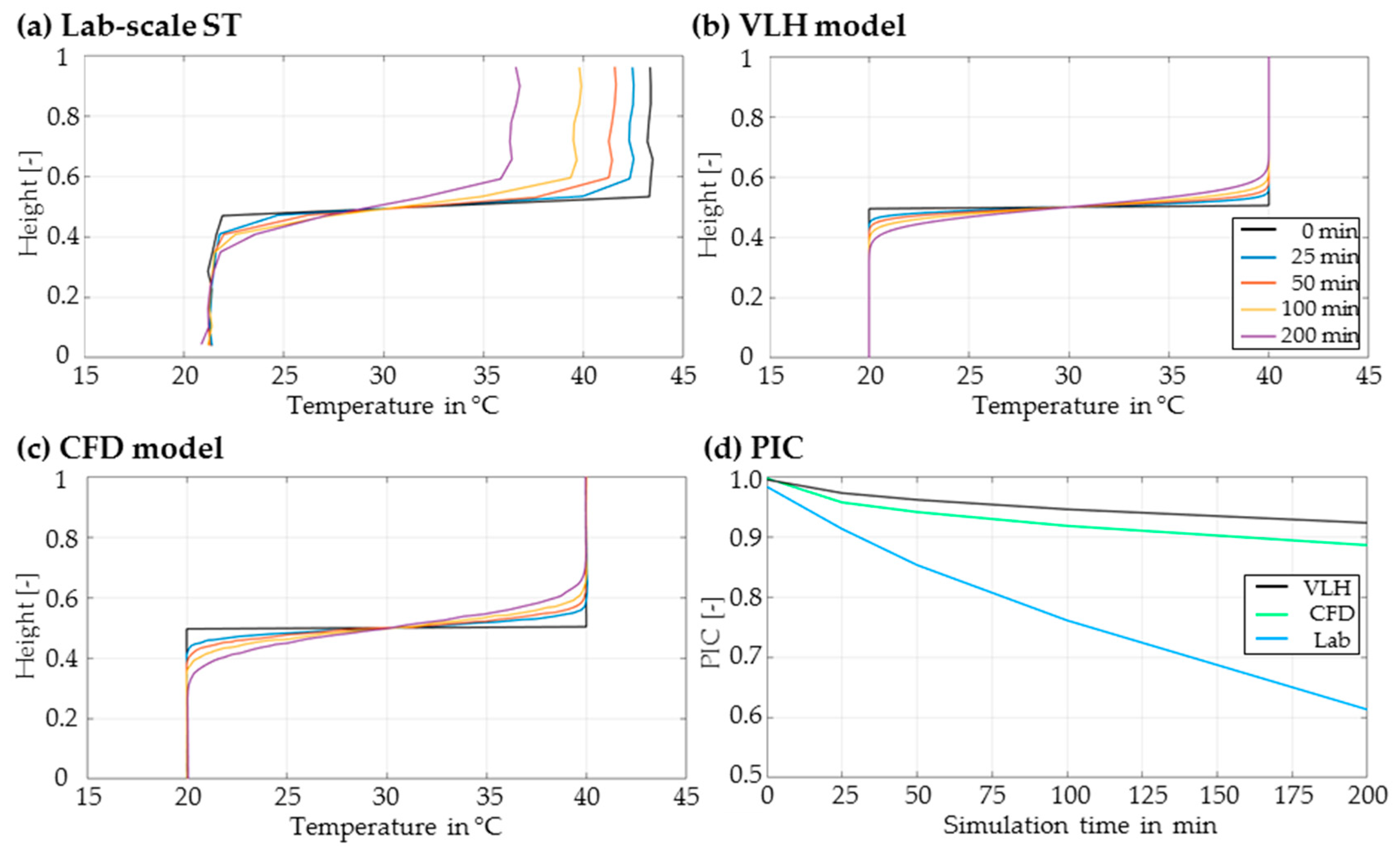
- The Static Mode investigates heat transfer mechanisms during a certain simulation time in a ST, with ideal stratification at the beginning, without inlet or outlet flows, and with (a) and without (b) heat losses. The loss of stratification by the numerical and physical diffusion effects is described by PIC.
- (2)
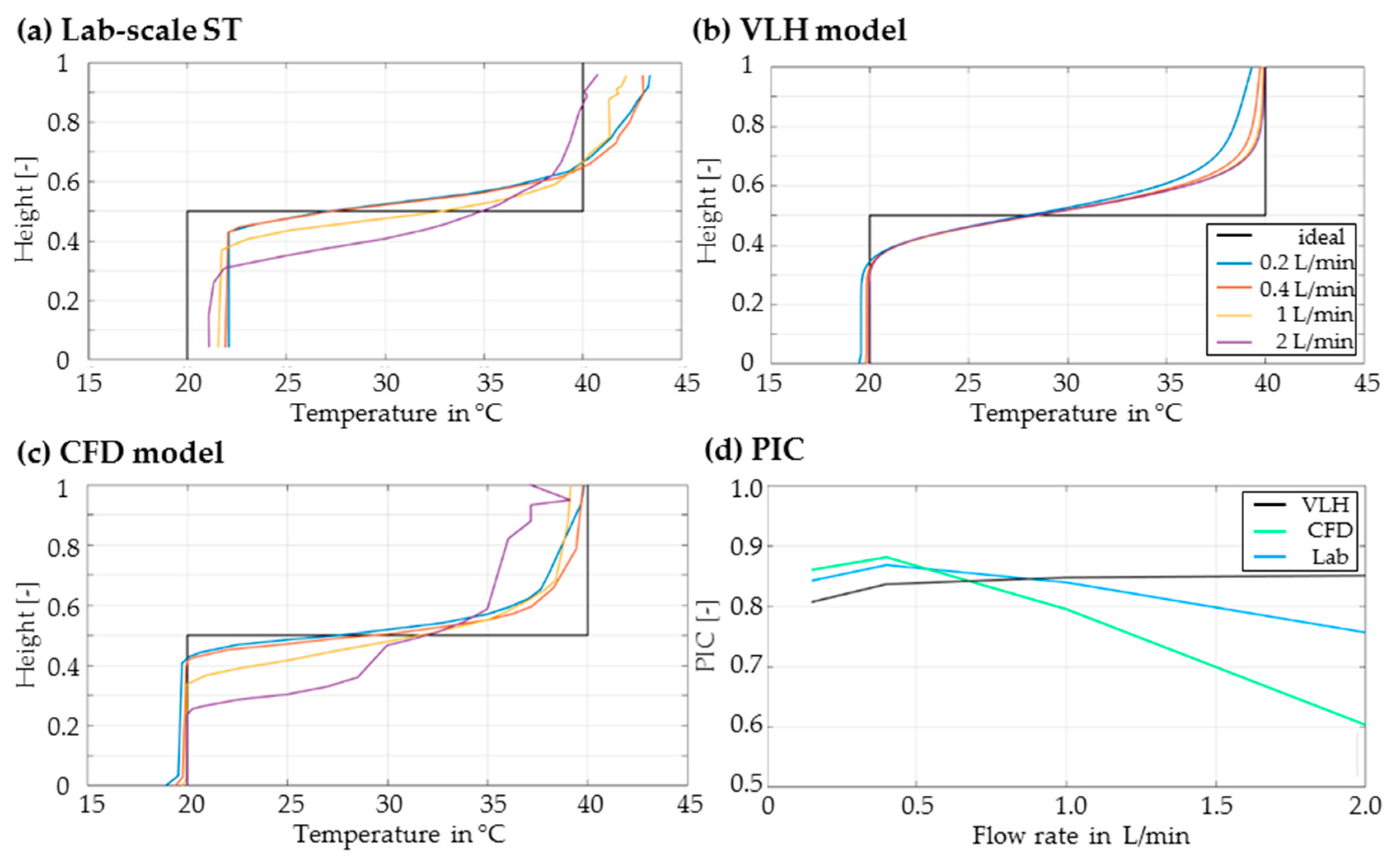
- Establishment of the thermocline by Charging studies the effect of the inlet flow rate of a charging process on the level of thermal stratification. In particular, the thermocline thickness and the location are observed. The tank is completely filled with cold water and warm water is supplied with different flow rates.
- (2)
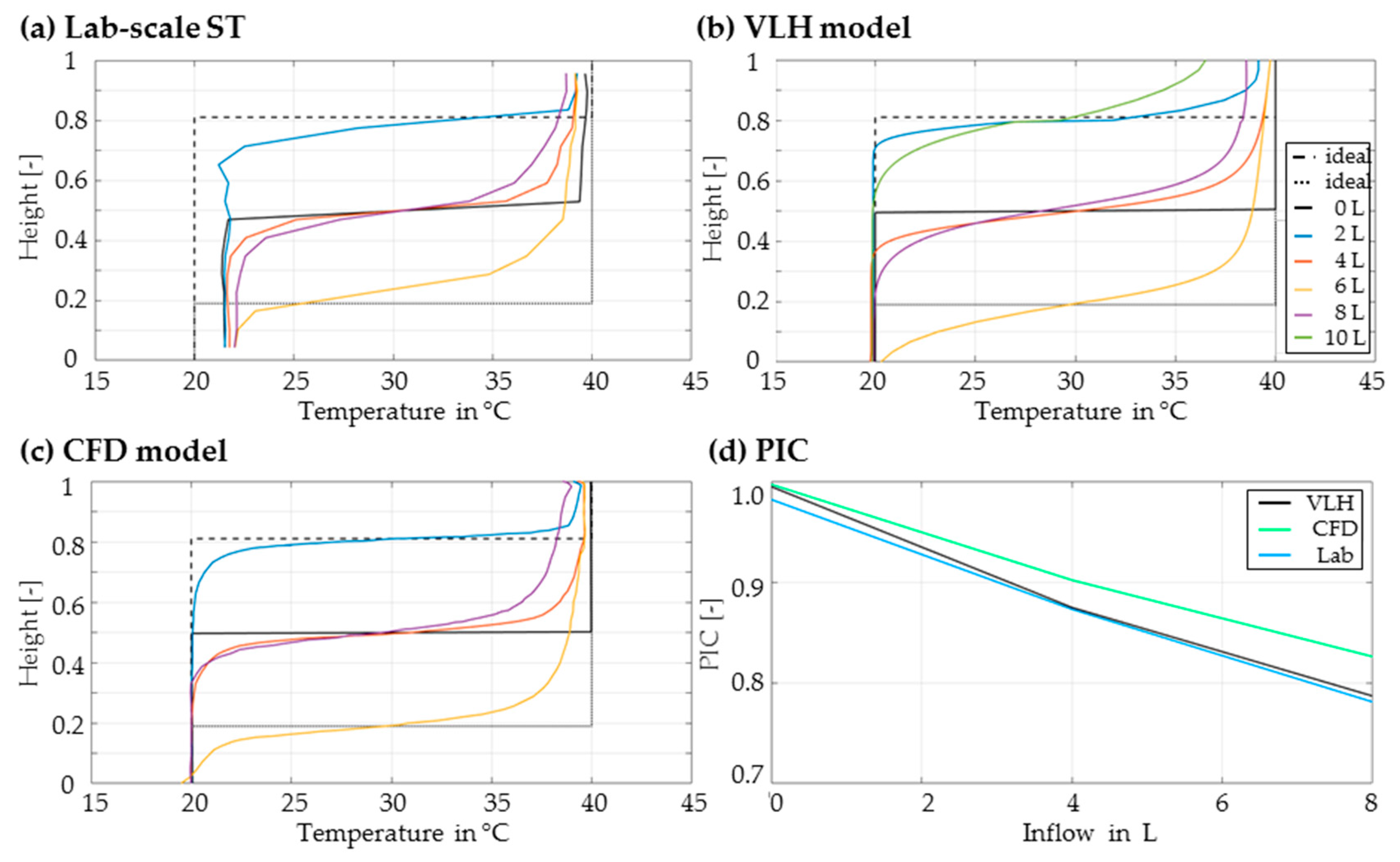
- Operating Mode Movement studies the effect a changing charging and discharging flow rates on the thermal thermocline position based on . Moreover, the degradation of stratification was measured by . The storage tank is alternately loaded and unloaded with 2 L cold, 4 L warm, and again 4 L cold water at a flow rate of 0.4 L/min.
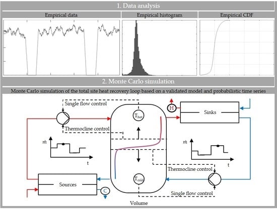
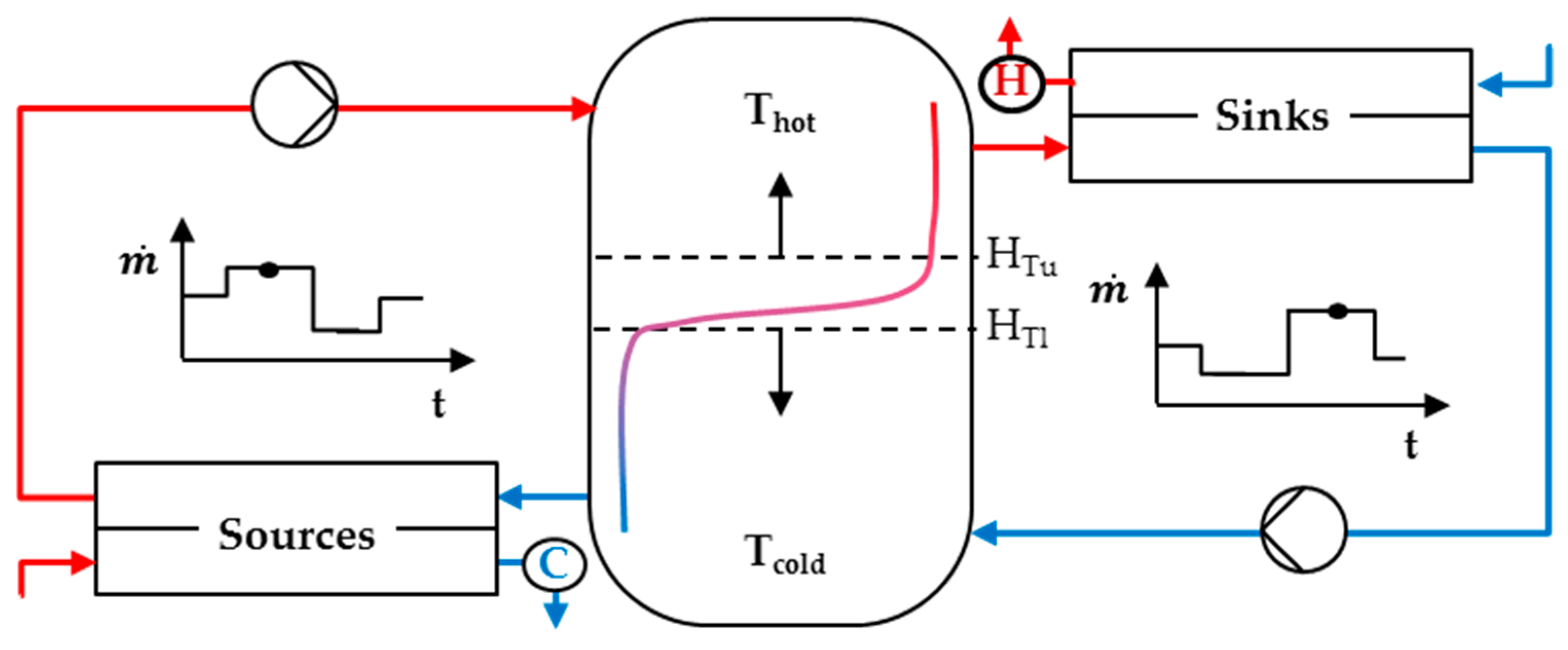
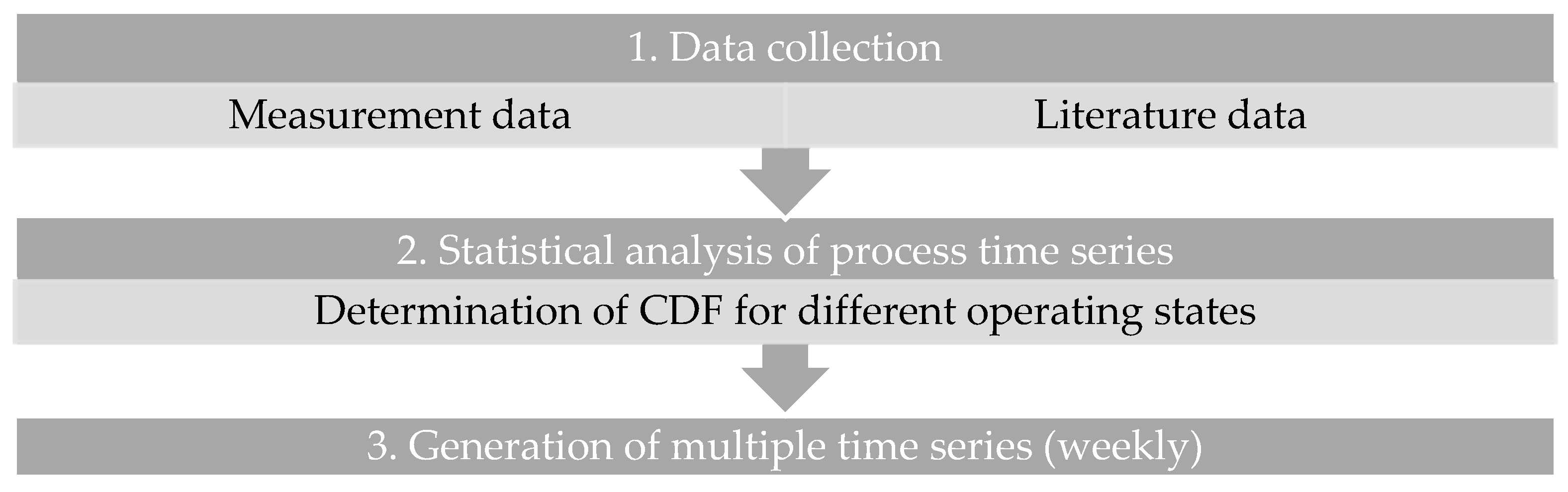
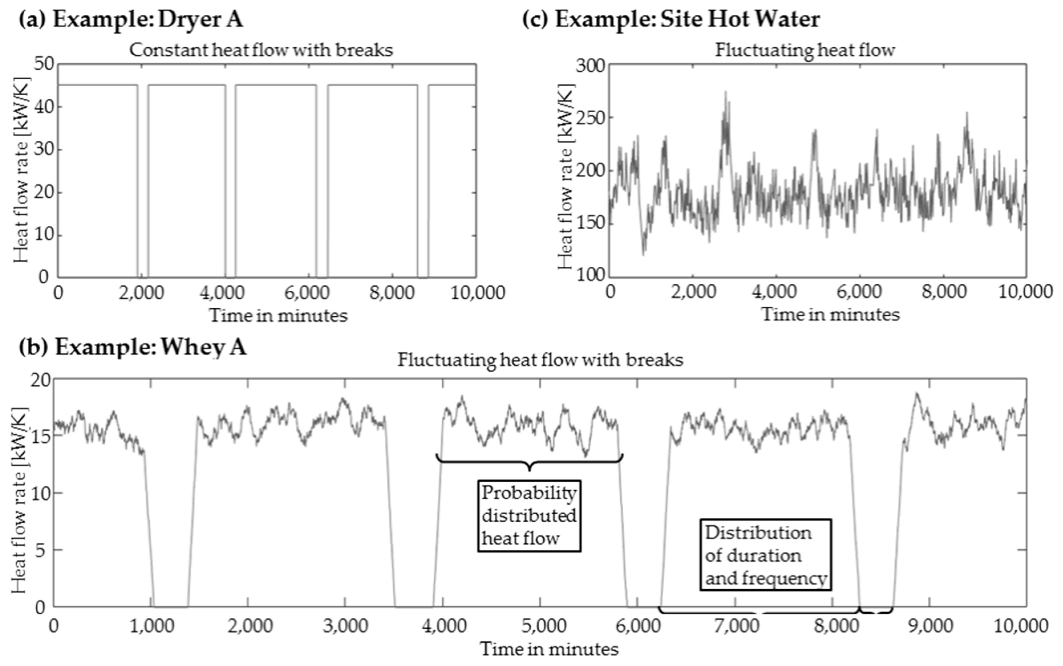
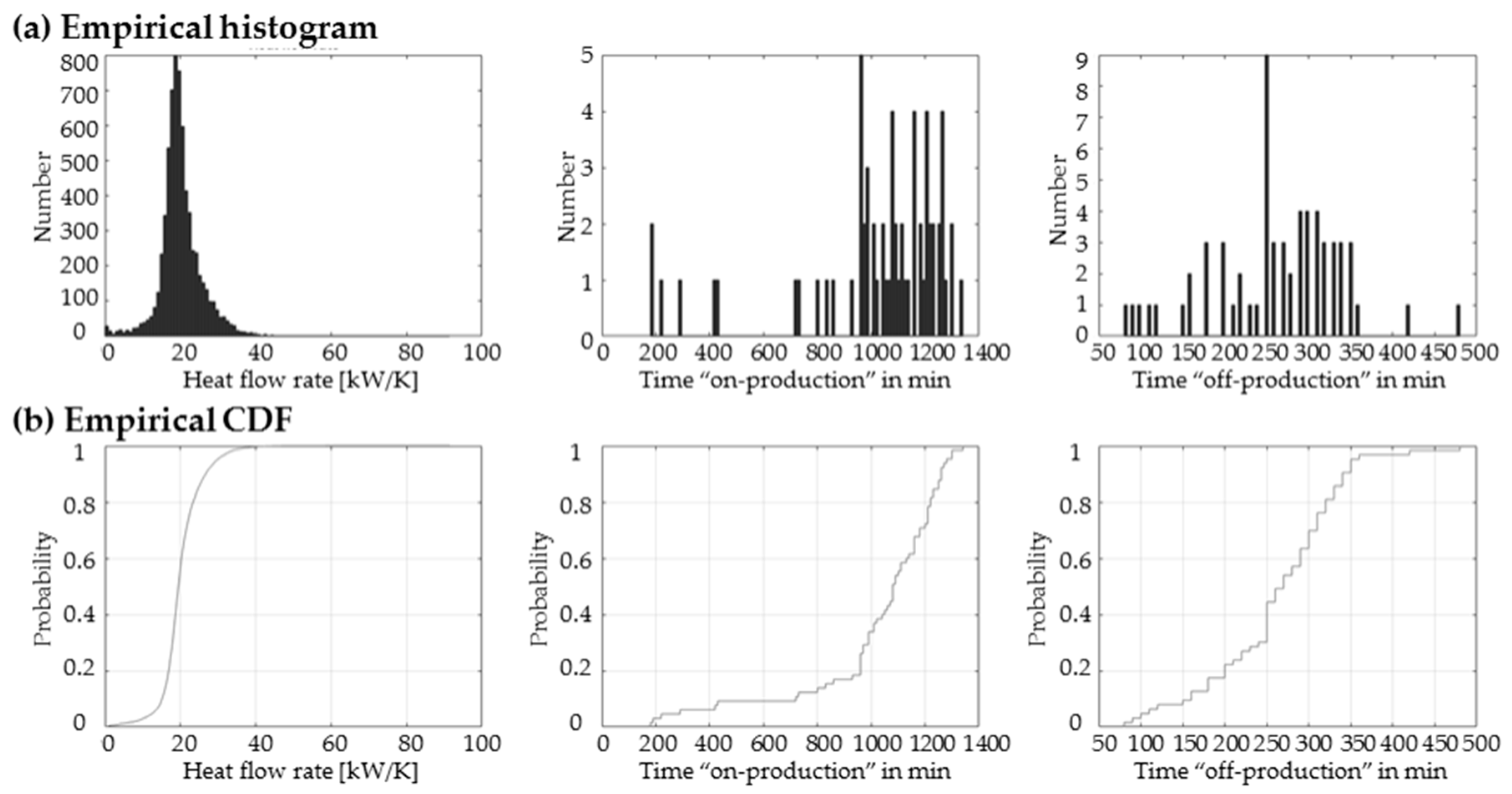
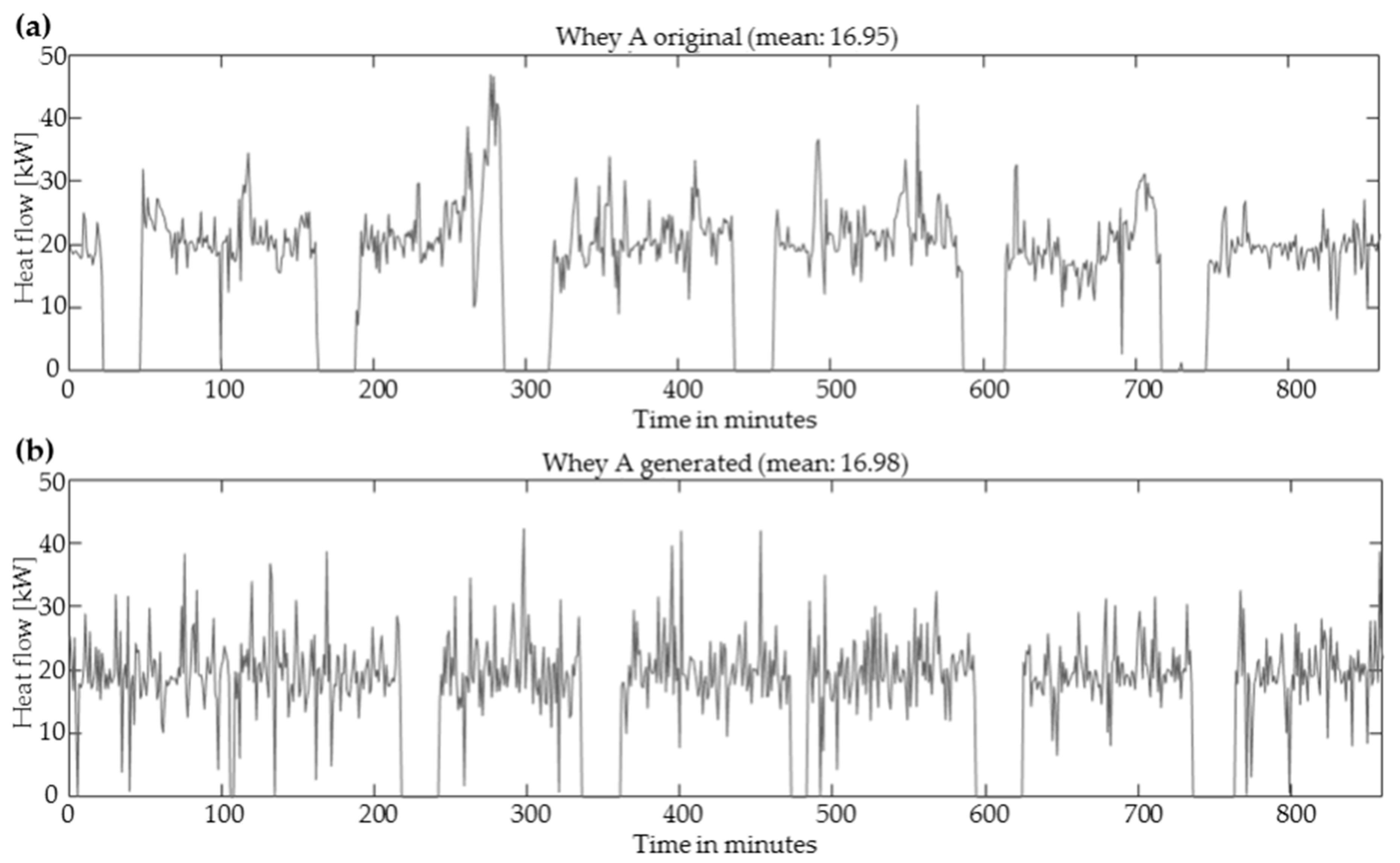
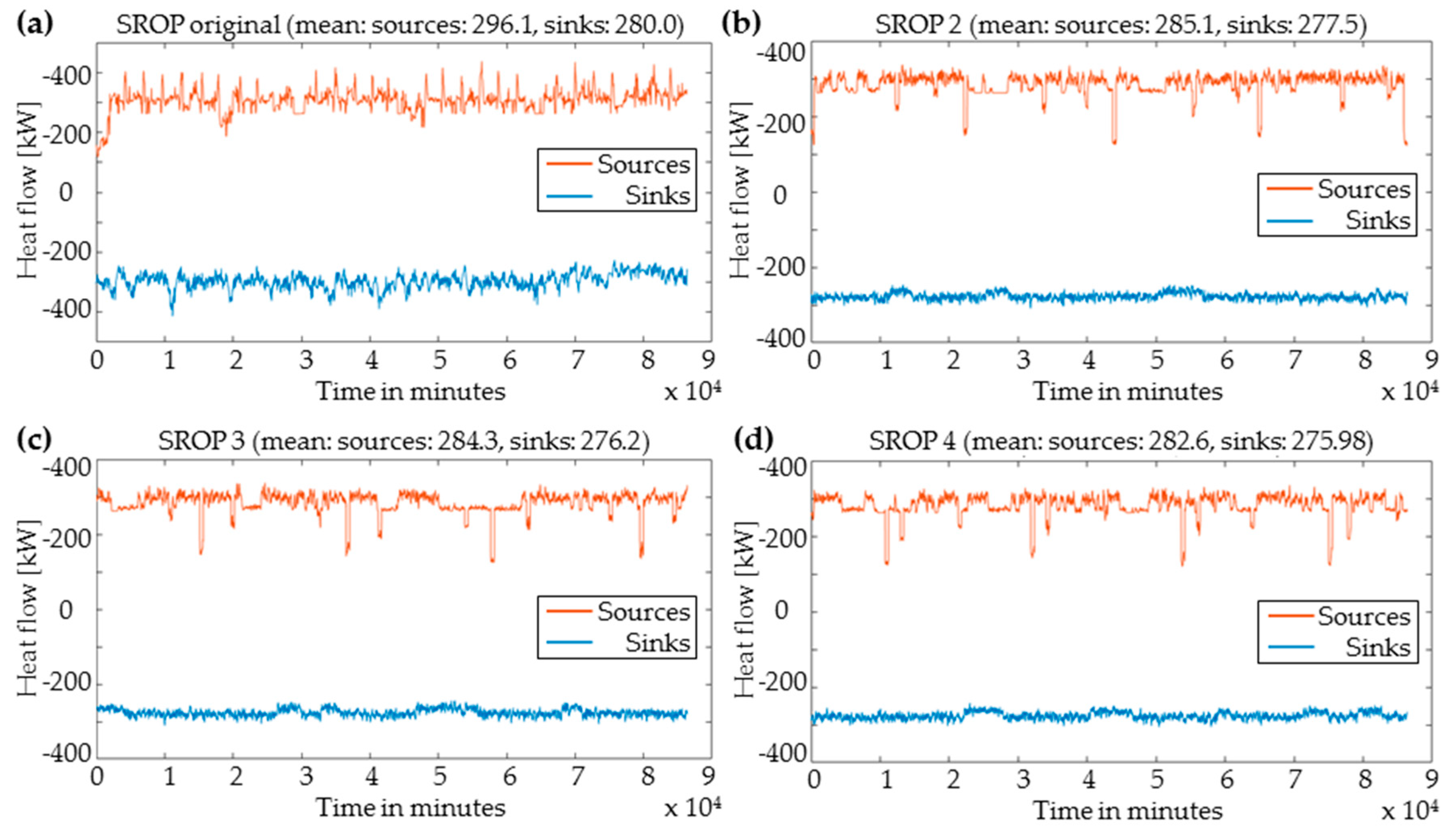
2.2. Generation of Stochastic Time Series for Monte Carlo Simulation
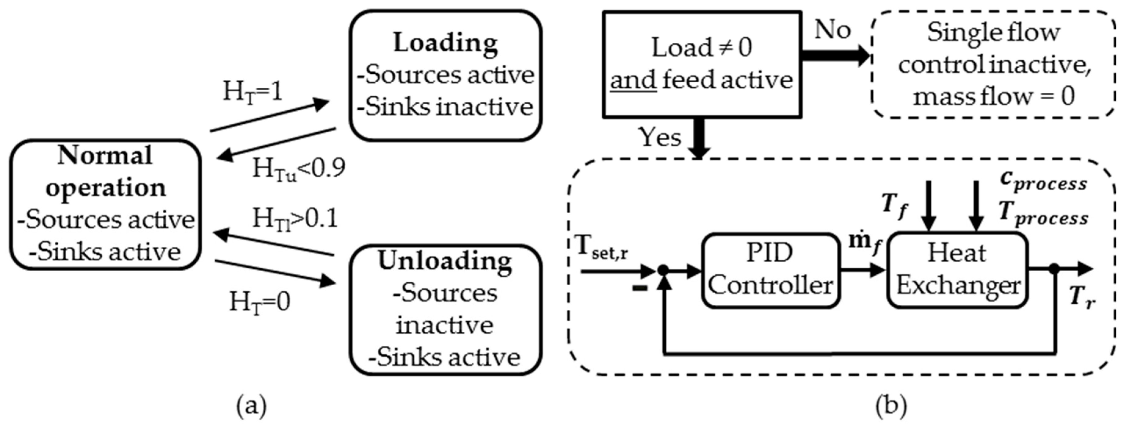
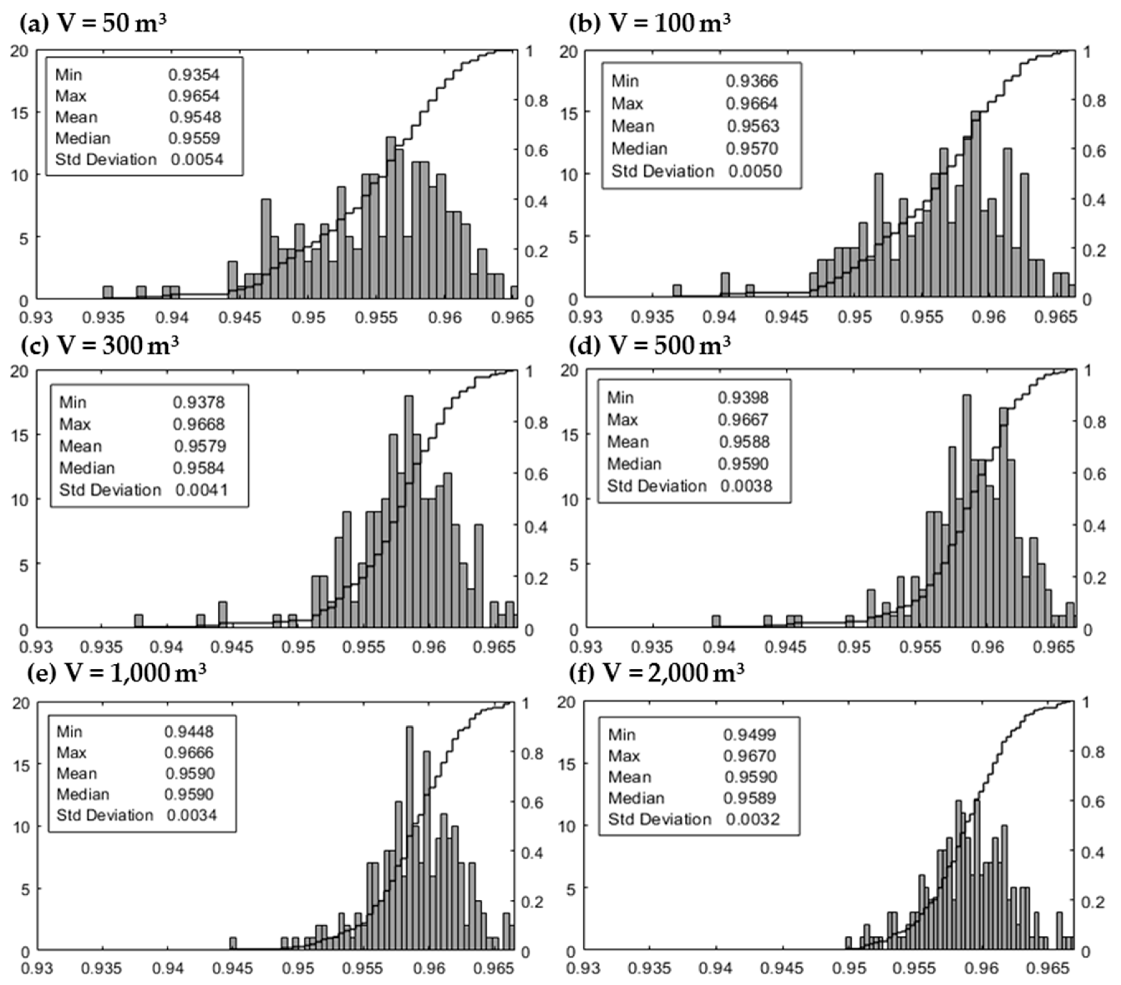
2.3. Evaluation of the Robust Heat Recovery Loop-Dimensioning via Dynamic Monte Carlo Simulation
3. Results
3.1. Validation of the Variable Layer Height Model
- (1)
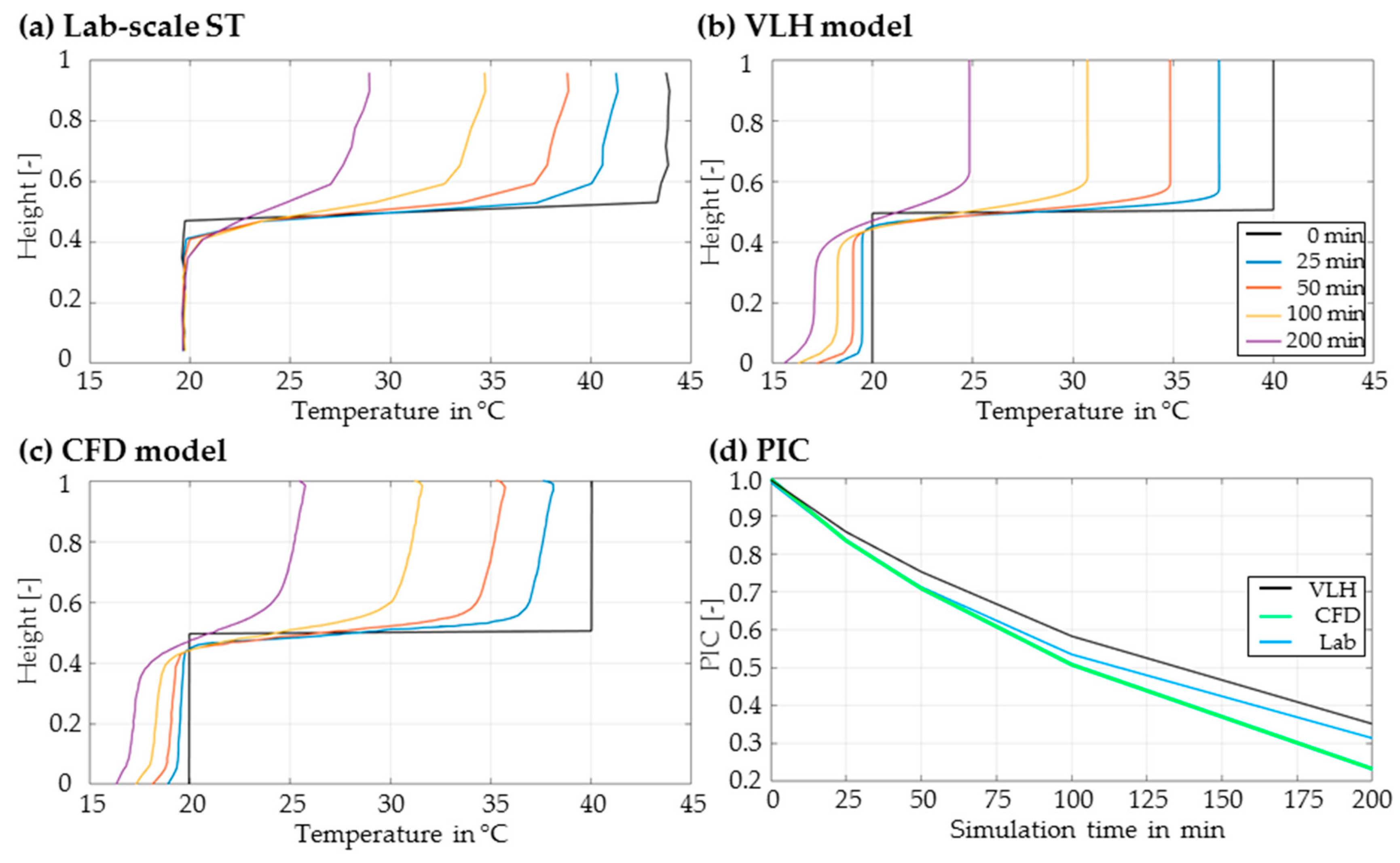
- (a) Static Mode: Numerical diffusion effects are reduced to an acceptable degree, as shown in the previous study [13]. For the lab tests, the heat losses cannot be eliminated completely by the thermal insulation. For all experiments (Figure 8a–c), the thermocline grows with the simulation duration due to numerical diffusion effects. The deviation from the ideal stratification (black line) measured by the PIC values thus also increases, as shown in Figure 8d. Using the VLH model, the influence of numerical diffusion is even lower than when using the CFD model.(b) Incoming or outgoing mass flows are still deactivated. Heat losses, on the other hand, are taken into account, which leads to the following destratification for different simulation times in Figure 9a–c. The destratification of the three models takes place to a similar extent in Figure 9d. Since no vertical heat conduction effects are taken into account for the MN approach, the stratification can only degrade evenly over the height (Figure 9b).
- (2)
- Establishment of the Thermocline by Charging: From a flow rate of over 1 L/min, turbulence causes destratification (Figure 10a,c). Therefore, the Courant condition has to be met, which states that a fluid particle should not move further than a node per time step. The destratification of the three models takes place to a similar extent until 1.0 L/min (Figure 10d). The degradation of the stratification of the CFD model and the lab-scale tank grows above this. On the other hand, the VLH model does not take turbulent flow forms into account, as seen in Figure 10b. For this reason, it can only be operated without restrictions up to a maximum inflow velocity of 0.002 m/s.
- (3)
- Operating Mode Movement: The thermocline initially moves upwards from its initial state by being filled with cold water (2 L). All models reach the expected position for the ideal behavior (black dotted lines in Figure 11a–c). After filling with warm water (4 L) the thermocline moves to the expected lower position. The storage tank is now filled to 81% with warm water. Subsequently, the predetermined heights are reached again when the tank is filled with cold water (4 L). The degradation of stratification generated by the flow rate can best be mapped by the VLH MN model (Figure 11d).
3.2. Stochastic Time Series of Dairy Plant
3.3. Evaluation of the Robust Heat Recovery Loop-Dimensioning via Monte Carlo Simulation
4. Discussion
5. Conclusions and Outlook
Author Contributions
Funding
Conflicts of Interest
Nomenclature
| A | Area |
| CC | Composite curve |
| CFD | Computational fluid dynamics |
| CDF | Cumulative distribution functions |
| CIP | Cleaning in place |
| FTVM | Fixed temperature, variable mass |
| Heat flow | |
| HRL | Heat recovery loop |
| HRR | Heat recovery rate |
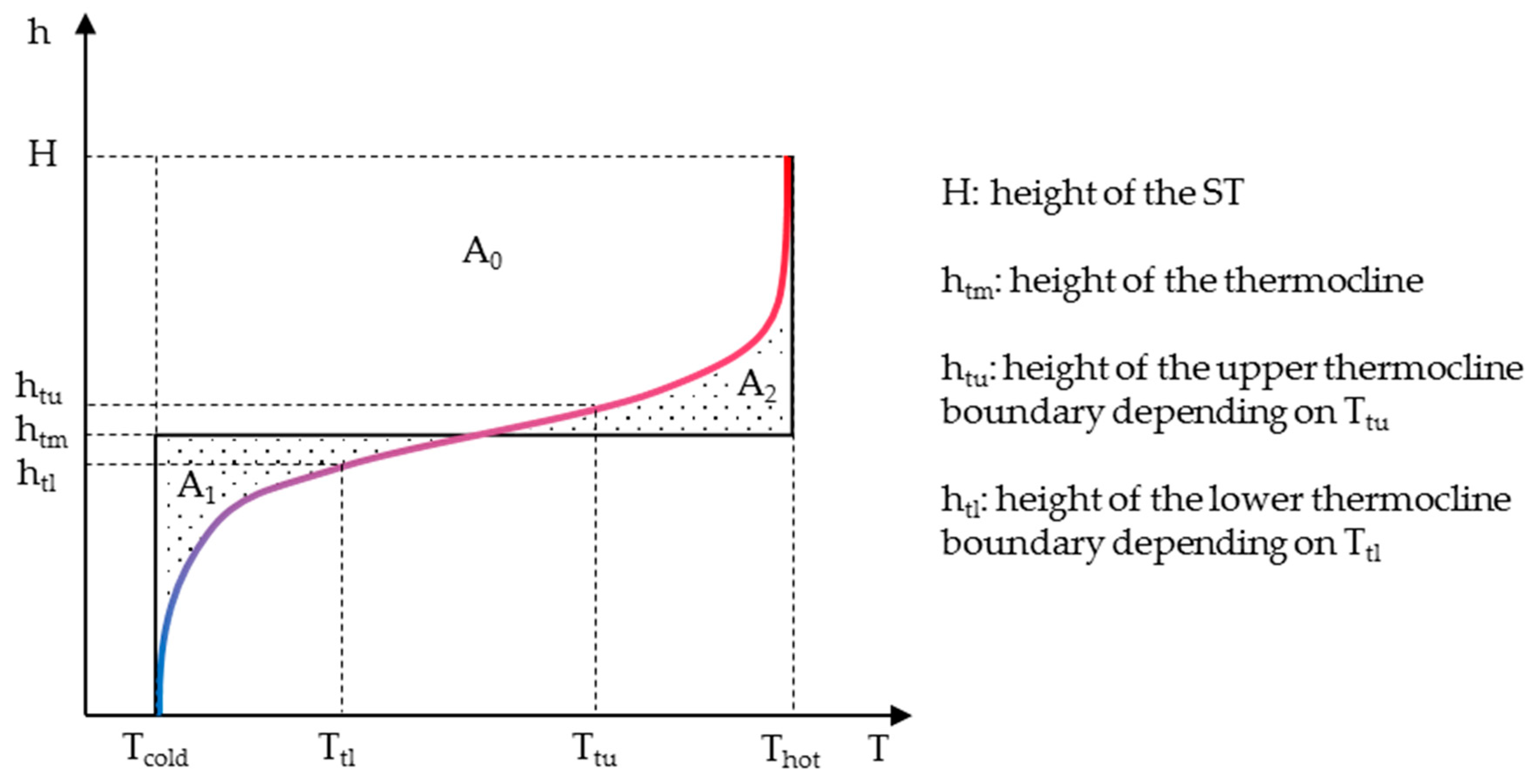
| H/htm | Medium height of the thermocline |
| H/htl | Lower height of the thermocline |
| H/htu | Upper height of the thermocline |
| ISSP | Indirect source and sink profile |
| Mass flow | |
| MC | Monte Carlo |
| MHR | Maximum heat recovery |
| MN | Multi-node |
| NTU | Number of transfer units |
| PIC | Percentage of ideal case |
| i | Thermal load |
| SROP | Stream-wise repeat operation period |
| ST | Stratified tank |
| t | Time |
| TAM | Time average model |
| Tcold | Temperature of the cold-water reservoir of a stratified tank |
| Thot | Temperature of the hot-water reservoir of a stratified tank |
| TSM | Time slice model |
| V | Volume |
| Volume flow | |
| VLH | Variable layer height |
| Heat flow rate |
References
- Eurostat. Energy Balance Sheets. 2015 Data. Statistical Books; Publications Office of the European Union: Luxembourg, 2017; ISBN 978-92-79-69844-6. [Google Scholar]
- Chan, Y.; Kantamaneni, R. Study on Energy Efficiency and Energy Saving Potential in Industry from possible Policy Mechanisms. 2015. Available online: https://ec.europa.eu/energy/sites/ener/files/documents/ 151201%20DG%20ENER%20Industrial%20EE%20study%20-%20final%20report_clean_stc.pdf (accessed on 28 November 2017).
- Philipp, M.; Schumm, G.; Peesel, R.-H.; Walmsley, T.G.; Atkins, M.J.; Schlosser, F.; Hesselbach, J. Optimal energy supply structures for industrial food processing sites in different countries considering energy transitions. Energy 2018, 146, 112–123. [Google Scholar] [CrossRef]
- Klemeš, J.J. Handbook of Process Integration: Minimisation of Energy and Water Use, Waste and Emissions; Woodhead Publishing: Cambridge, UK, 2013; ISBN 9780857095930. [Google Scholar]
- Klemeš, J.; Dhole, V.R.; Raissi, K.; Perry, S.J.; Puigjaner, L. Targeting and design methodology for reduction of fuel, power and CO2 on total sites. Appl. Therm. Eng. 1997, 17, 993–1003. [Google Scholar] [CrossRef]
- Schumm, G.; Philipp, M.; Schlosser, F.; Hesselbach, J.; Walmsley, T.G.; Atkins, M.J. Hybrid-heating-systems for optimized integration of low-temperature-heat and renewable energy. Chem. Eng. Trans. 2016, 52, 1087–1092. [Google Scholar] [CrossRef]
- Walmsley, T.G.; Walmsley, M.R.W.; Tarighaleslami, A.H.; Atkins, M.J.; Neale, J.R. Integration options for solar thermal with low temperature industrial heat recovery loops. Energy 2015, 90, 113–121. [Google Scholar] [CrossRef]
- Olsen, D.; Liem, P.; Abdelouadoud, Y.; Wellig, B. Thermal energy storage integration based on pinch analysis—Methodology and application. Chem. Ing. Tech. 2017, 89, 598–606. [Google Scholar] [CrossRef]
- Krummenacher, P. Contribution to the Heat Integration of Batch Processes (with or without Heat Storage). Ph.D. Thesis, École Polytechnique Fédérale de Lausanne, Lausanne, Switzerland, 2002. [Google Scholar]
- Atkins, M.J.; Walmsley, M.R.W.; Neale, J.R. The challenge of integrating non-continuous processes—Milk powder plant case study. J. Clean. Prod. 2010, 18, 927–934. [Google Scholar] [CrossRef]
- Walmsley, T.G.; Walmsley, M.R.W.; Atkins, M.J.; Neale, J.R. Integration of industrial solar and gaseous waste heat into heat recovery loops using constant and variable temperature storage. Energy 2014, 75, 53–67. [Google Scholar] [CrossRef]
- Atkins, M.J.; Walmsley, M.R.W.; Neale, J.R. Process integration between individual plants at a large dairy factory by the application of heat recovery loops and transient stream analysis. J. Clean. Prod. 2012, 34, 21–28. [Google Scholar] [CrossRef]
- Walmsley, M.R.W.; Atkins, M.J.; Riley, J. Thermocline management of stratified tanks for heat storage. Chem. Eng. Trans. 2009, 18, 231–236. [Google Scholar]
- Baeten, B.; Confrey, T.; Pecceu, S.; Rogiers, F.; Helsen, L. A validated model for mixing and buoyancy in stratified hot water storage tanks for use in building energy simulations. Appl. Energy 2016, 172, 217–229. [Google Scholar] [CrossRef]
- Campos Celador, A.; Odriozola, M.; Sala, J.M. Implications of the modelling of stratified hot water storage tanks in the simulation of CHP plants. Energy Convers. Manag. 2011, 52, 3018–3026. [Google Scholar] [CrossRef]
- Powell, K.M.; Edgar, T.F. An adaptive-grid model for dynamic simulation of thermocline thermal energy storage systems. Energy Convers. Manag. 2013, 76, 865–873. [Google Scholar] [CrossRef]
- Schlosser, F.; Peesel, R.-H.; Meschede, H.; Philipp, M.; Walmsley, T.G. Evaluation of a stratified tank based heat recovery loop via dynamic simulation. Chem. Eng. Trans. 2018, 70, 403–408. [Google Scholar] [CrossRef]
- Meschede, H.; Dunkelberg, H.; Stöhr, F.; Peesel, R.-H.; Hesselbach, J. Assessment of probabilistic distributed factors influencing renewable energy supply for hotels using Monte-Carlo methods. Energy 2017, 128, 86–100. [Google Scholar] [CrossRef]
- Lal, N.S.; Atkins, M.J.; Walmsley, M.R.W.; Walmsley, T.G. Accounting for stream variability in retrofit problems using Monte Carlo simulation. Chem. Eng. Trans. 2018, 70, 1015–1020. [Google Scholar] [CrossRef]
- Walmsley, M.R.W.; Atkins, M.J.; Linder, J.; Neale, J.R. Thermocline movement dynamics and thermocline growth in stratified tanks for heat storage. Chem. Eng. Trans. 2010, 21, 991–996. [Google Scholar] [CrossRef]
- Rabe, M.; Spieckermann, S.; Wenzel, S. Verifikation und Validierung für die Simulation in Produktion und Logistik. Vorgehensmodelle und Techniken; Springer: Berlin, Germany, 2008; ISBN 978-3-540-35282-2. [Google Scholar]
- Dufo-López, R.; Pérez-Cebollada, E.; Bernal-Agustín, J.L.; Martínez-Ruiz, I. Optimisation of energy supply at off-grid healthcare facilities using Monte Carlo simulation. Energy Convers. Manag. 2016, 113, 321–330. [Google Scholar] [CrossRef]
- Dunkelberg, H.; Sondermann, M.; Meschede, H.; Hesselbach, J. Assessment of flexibilisation potential by changing energy sources using Monte Carlo simulation. Energies 2019, 12, 711. [Google Scholar] [CrossRef]
- Nijhuis, M.; Gibescu, M.; Cobben, J.F.G. Bottom-up Markov chain Monte Carlo approach for scenario based residential load modelling with publicly available data. Energy Build. 2016, 112, 121–129. [Google Scholar] [CrossRef]
- VDI. VDI-Wärmeatlas. Mit 320 Tabellen; Springer Vieweg: Berlin, Germany, 2013; ISBN 3642199801. [Google Scholar]


| Number | Validation Experiment | Physical Modelling | Simulation Time | ||||||
|---|---|---|---|---|---|---|---|---|---|
| L/min | - | m | min | ||||||
| 1a | Static Mode | Adiabatic | - | 40 | 20 | 0.5 | 0 | 200 | |
| 1b | Non-adiabatic | - | 40 | 20 | 15 | 0.5 | 0 | 200 | |
| 2a | Charging | Constant charging with 40 °C | 0.15 | 20 | 20 | 15 | 1.0 | 0 | 26.7 |
| 2b | 0.4 | 10.0 | |||||||
| 2c | 1.0 | 4.0 | |||||||
| 2d | 2.0 | 2.0 | |||||||
| 3 | Movement | Sequentially charging | 0.4 | 40 | 20 | 15 | 0.5 | 0 | 25 |
| Process | Type | ||||||
|---|---|---|---|---|---|---|---|
| Utility | Hot 1 | 50 | 30 | 10 | 195 | 8 | 160 |
| Casein | Hot 2 | 50 | 20 | 49 | 1477 | 32 | 956 |
| Dryer A | Hot 3 | 55 | 10 | 143 | 6415 | 139 | 6266 |
| Dryer B | Hot 4 | 55 | 10 | 75 | 3368 | 73 | 3290 |
| Dryer C | Hot 5 | 55 | 10 | 45 | 2020 | 44 | 1973 |
| Milk Treatment | Cold 1 | 10 | 55 | 90 | 4057 | 90 | 4057 |
| Whey | Cold 2 | 12 | 50 | 20 | 763 | 16 | 601 |
| Site Hot Water | Cold 3 | 15 | 65 | 160 | 7987 | 160 | 7987 |
© 2019 by the authors. Licensee MDPI, Basel, Switzerland. This article is an open access article distributed under the terms and conditions of the Creative Commons Attribution (CC BY) license (http://creativecommons.org/licenses/by/4.0/).
Share and Cite
Schlosser, F.; Peesel, R.-H.; Meschede, H.; Philipp, M.; Walmsley, T.G.; Walmsley, M.R.W.; Atkins, M.J. Design of Robust Total Site Heat Recovery Loops via Monte Carlo Simulation. Energies 2019, 12, 930. https://doi.org/10.3390/en12050930
Schlosser F, Peesel R-H, Meschede H, Philipp M, Walmsley TG, Walmsley MRW, Atkins MJ. Design of Robust Total Site Heat Recovery Loops via Monte Carlo Simulation. Energies. 2019; 12(5):930. https://doi.org/10.3390/en12050930
Chicago/Turabian StyleSchlosser, Florian, Ron-Hendrik Peesel, Henning Meschede, Matthias Philipp, Timothy G. Walmsley, Michael R. W. Walmsley, and Martin J. Atkins. 2019. "Design of Robust Total Site Heat Recovery Loops via Monte Carlo Simulation" Energies 12, no. 5: 930. https://doi.org/10.3390/en12050930